Hadronic decays of the (pseudo-)scalar charmonium states $\eta_{c}$ and $\chi_{c0}$ in the extended Linear Sigma Model

Abstract

We study the phenomenology of the ground-state (pseudo-)scalar charmonia $\eta_{c}$ and $\chi_{c0}$ in the framework of a $U(4)_{r}\times U(4)_{l}$ symmetric linear sigma model with (pseudo-)scalar and (axial-) vector mesons. Based on previous results for the spectrum of charmonia and the spectrum and (OZI-dominant) strong decays of open charmed mesons, we extend the study of this model to OZI-suppressed charmonia decays. This includes decays into ’ordinary’ mesons but also particularly interesting channels with scalar-isoscalar resonances $f_{0}(1370),\,f_{0}(1500),\,f_{0}(1710)$ that may include sizeable contributions from a scalar glueball. We study the variation of the corresponding decay widths assuming different mixings between glueball and quark-antiquark states. We also compute the decay width of the pseudoscalar $\eta_{c}$ into a pseudoscalar glueball. In general, our results for decay widths are in reasonable agreement with experimental data where available. Order of magnitude predictions for as yet unmeasured states and channels are potentially interesting for BESIII, Belle II, LHCb as well as the future PANDA experiment at the FAIR facility.

I Introduction

In recent years, the charm quark energy region has been the focus of many theoretical and experimental investigations Patrignani et al. (2016). In particular the plethora of recently discovered exotic states, i.e. states with quark content beyond $q\bar{q}$ and $qqq$ or states with quantum numbers not accounted for in non-relativistic quark models, have raised enormous interest. With the copious production of ’ordinary’ charmonia in experiments such as BESIII, Belle (II) and LHCb, however, also their potentially rare decays into light hadrons gains interest. These transitions occur via gluon-rich processes and are therefore interesting with respect to the interplay and transition of perturbative and non-perturbative QCD. Consequently, theoretical work in the past has concentrated on the application and limits of perturbative QCD and the construction of non-perturbative models for the (OZI-suppressed) production of $q\bar{q}$-pairs in the decays, see e.g. Bodwin et al. (1992); Zhou et al. (2005); Close and Zhao (2005); Zhao (2008); Segovia et al. (2013); Frere and Heeck (2015) and Refs. therein.

Exotic states, however not only occur in the charm quark region, but may be present already in the light quark sector. In particular the light scalar meson sector is discussed frequently, with a putative scalar isoscalar glueball in the energy region around 1.5 GeV. The decay of charmonia into pairs of these states may offer the interesting possibility to study the nature of these states using information from the gluon-rich decay processes.

In order to study these decays we employ the extended Linear Sigma Model (eLSM) Ko and Rudaz (1994); Urban et al. (2002), an effective model describing the vacuum phenomenology of (pseudo-)scalar and (axial-)vector mesons in the cases of $N_{f}=2$ Parganlija et al. (2010); Gallas et al. (2010); Janowski et al. (2011) and $N_{f}=3$ Parganlija et al. (2013). Recently, the framework has been generalised to $N_{f}=4$ Eshraim (2013); Eshraim and Giacosa (2014); Eshraim (2015a, b); Eshraim et al. (2015); Eshraim (2015c) and applied to the calculation of masses of open and hidden charmed mesons as well as the decays of open charmed mesons in the low energy limit. Although the model is rooted in chiral symmetry and its breaking pattern in the light quark sector, these applications have been (perhaps unexpectedly) quite successful. In this work we extend these studies to also include the decays of hidden charm mesons.

The construction of the eLSM is based on a global chiral symmetry $U(N_{f})_{r}\times U(N_{f})_{l}$ as well as the classical dilation symmetry. In the vacuum, global chiral symmetry is broken spontaneously by a non-vanishing expectation value of the quark condensate, anomalously by quantum effects, and explicitly by non-vanishing quark masses. Furthermore, the dilation symmetry is broken explicitly. As a consequence, besides the usual meson multiplets the eLSM also includes two glueballs composed of two gluons each: a scalar one (denoted as $G$) Rosenzweig et al. (1981); Migdal and Shifman (1982); Gomm et al. (1986); Gomm and Schechter (1985) and a pseudoscalar one (denoted as $\widetilde{G}$). The identification of the scalar glueballs with experimentally observed states is notoriously complicated, see e.g. Amsler and Close (1996); Lee and Weingarten (2000); Close and Kirk (2001); Amsler and Tornqvist (2004); Giacosa et al. (2005a, b); Cheng et al. (2006); Klempt and Zaitsev (2007); Chatzis et al. (2011) for discussions. In general, there is a mixing between states: the non-strange $\sigma_{N}\equiv(u\overline{u}+d\overline{d})/\sqrt{2}$, hidden-strange $\sigma_{S}\equiv s\overline{s}$, and scalar glueball $G\equiv gg$ Close and Zhao (2005); Zhao (2008); Frere and Heeck (2015). Within the eLSM this three-body mixing in the scalar-isoscalar channel was resolved in Ref. Janowski et al. (2011, 2014) and generated the physical resonances $f_{0}(1370),\,f_{0}(1500)$ and $f_{0}(1710)$. Of these, the $f_{0}(1710)$ has the largest overlap with the scalar glueball. Its counterpart in the pseudoscalar sector has been studied within the eLSM in Refs. Eshraim et al. (2013, 2012); Eshraim and Janowski (2012, 2013); Eshraim and Schramm (2017). In the charm sector, the eLSM contains so far four charmonium states, which are (pseudo-)scalar and (axial-)vector ground states $\eta_{c},\chi_{c0},J/\psi(1S)$ and $\chi_{c1}$ Eshraim et al. (2015). In the present work we study the OZI-suppressed decays of the two (pseudo-)scalar charmonia.

We use eLSM parameters in the light, strange and charm quark sectors fixed previously Parganlija et al. (2013); Eshraim et al. (2015). In addition we introduce two new parameters, $\lambda_{1}^{C},\,h_{1}^{C}$, which control the decay widths of $\eta_{c}$ and $\chi_{c0}$. This, together with a summary of the construction of the eLSM is discussed in section II. In section III we present the results of the two- and three-body decay widths of $\eta_{c}$ and $\chi_{c0}$, and discuss their significance. In section IV we conclude. Details of the calculations are relegated to the Appendices.

II The $U(4)_{r}\times U(4)_{l}$ LSM interaction with glueballs

The $U(4)_{L}\times U(4)_{R}$ linear sigma model with (pseudo)scalar and (axial-)vector mesons, a scalar $G$ and a pseudoscalar glueball $\widetilde{G}$ is given by Eshraim et al. (2015)

$$\mathcal{L} =\mathcal{L}_{dil}+\mathrm{Tr}[(D^{\mu}\Phi)^{\dagger}(D^{\mu}\Phi)]-m_{0}^{2}\left(\frac{G}{G_{0}}\right)^{2}\mathrm{Tr}(\Phi^{\dagger}\Phi)-\lambda_{1}^{S}[\mathrm{Tr}((\mathbbm{1}-\mathbb{P}_{C})\Phi^{\dagger}(\mathbbm{1}-\mathbb{P}_{C})\Phi)]^{2}-\lambda_{1}^{C}[\mathrm{Tr}(\Phi^{\dagger}\Phi)]^{2}$$

$$-\lambda_{2}\mathrm{Tr}(\Phi^{\dagger}\Phi)^{2}+\mathrm{Tr}\left\{\left[\left(\frac{G}{G_{0}}\right)^{2}\frac{m_{1}^{2}}{2}+\Delta\right]\left[(L^{\mu})^{2}+(R^{\mu})^{2}\right]\right\}-\frac{1}{4}\mathrm{Tr}[(L^{\mu\nu})^{2}+(R^{\mu\nu})^{2}]-2\,\mathrm{Tr}[\varepsilon\Phi^{\dagger}\Phi]$$

$$+\mathrm{Tr}[H(\Phi+\Phi^{\dagger})]+c(det\Phi-det\Phi^{\dagger})^{2}-\delta\widetilde{c}(det\Phi-det\Phi^{\dagger})^{2}\mathrm{Tr}(\mathbb{P}_{C}\Phi^{\dagger}\mathbb{P}_{C}\Phi)+i\tilde{c}\,\tilde{G}\left(\text{{det}}\Phi-\text{{det}}\Phi^{{\dagger}}\right)$$

$$+\frac{h_{1}^{S}}{2}\mathrm{Tr}((\mathbbm{1}-\mathbb{P}_{C})\Phi^{\dagger}(\mathbbm{1}-\mathbb{P}_{C})\Phi)\mathrm{Tr}[(L^{\mu})^{2}+(R^{\mu})^{2}]+\frac{h_{1}^{C}}{2}\mathrm{Tr}(\Phi^{\dagger}\Phi)\mathrm{Tr}[(L^{\mu})^{2}+(R^{\mu})^{2}]$$

$$+h_{2}\mathrm{Tr}[(\Phi R^{\mu})^{2}+(L^{\mu}\Phi)^{2}]+2h_{3}\mathrm{Tr}(\Phi R_{\mu}\Phi^{\dagger}L^{\mu})$$

$$+i\frac{g_{2}}{2}\{\mathrm{Tr}(L_{\mu\nu}[L^{\mu},L^{\nu}])+\mathrm{Tr}(R_{\mu\nu}[R^{\mu},R^{\nu}])\}+...\text{ ,}$$ (1)

where $D^{\mu}\Phi\equiv\partial^{\mu}\Phi-ig_{1}(L^{\mu}\Phi-\Phi R^{\mu})$ is the covariant derivative; $L^{\mu\nu}\equiv\partial^{\mu}L^{\nu}-\partial^{\nu}L^{\mu}$, and $R^{\mu\nu}\equiv\partial^{\mu}R^{\nu}-\partial^{\nu}R^{\mu}$ are the left-handed and right-handed field strength tensors. In addition to chiral symmetry it features dilatation invariance and invariance under the discrete symmetries $C$ and $P$. In the following we summarise the most important features of the so defined extended linear sigma model (eLSM).

In our framework with $N_{f}=4$ quark flavours the field $\Phi$ represents the $4\times 4$ (pseudo)scalar multiplets

$$\Phi=(S^{a}+iP^{a})t^{a}=\frac{1}{\sqrt{2}}\left(\begin{array}[]{cccc}\frac{(\sigma_{N}+a^{0}_{0})+i(\eta_{N}+\pi^{0})}{\sqrt{2}}&a^{+}_{0}+i\pi^{+}&K^{*+}_{0}+iK^{+}&D^{*0}_{0}+iD^{0}\\ a^{-}_{0}+i\pi^{-}&\frac{(\sigma_{N}-a^{0}_{0})+i(\eta_{N}-\pi^{0})}{\sqrt{2}}&K^{*0}_{0}+iK^{0}&D^{*-}_{0}+iD^{-}\\ K^{*-}_{0}+iK^{-}&\overline{K}^{*0}_{0}+i\overline{K}^{0}&\sigma_{S}+i\eta_{S}&D^{*-}_{S0}+iD^{-}_{S}\\ \overline{D}^{*0}_{0}+i\overline{D}^{0}&D^{*+}_{0}+iD^{+}&D^{*+}_{S0}+iD^{+}_{S}&\chi_{C0}+i\eta_{C}\\ \end{array}\right),$$ (2)

where $t^{a}$ are the generators of the group $U(N_{f})$. The multiplet $\Phi$ transforms as $\Phi\rightarrow U_{L}\Phi U_{R}^{\dagger}$ under $U_{L}(4)\times U_{R}(4)$ chiral transformations with $U_{L(R)}=e^{-i\theta_{L(R)}^{a}t^{a}}$, with $\Phi(t,\vec{x})\rightarrow\Phi^{\dagger}(t,-\vec{x})$ under parity transformations, and $\Phi\rightarrow\Phi^{\dagger}$ under charge conjugation. The determinant of $\Phi$ is invariant under $SU(4)_{L}\times SU(4)_{R}$, but not under $U(1)_{A}$ because ${\rm det\Phi}\rightarrow{\rm det}U_{A}\Phi U_{A}=e^{-i\theta_{A}^{0}\sqrt{2N_{f}}}{\rm det\Phi}\neq{\rm det\Phi}$.

Next we present the left- and right-handed (axial)vector multiplets $L^{\mu}$ and $R^{\mu}$ containing the vector and axial-vector degrees of freedom $V^{a}$ and $A^{a}$

$$L^{\mu}=(V^{a}+i\,A^{a})^{\mu}\,t^{a}=\frac{1}{\sqrt{2}}\left(\begin{array}[]{cccc}\frac{\omega_{N}+\rho^{0}}{\sqrt{2}}+\frac{f_{1N}+a_{1}^{0}}{\sqrt{2}}&\rho^{+}+a^{+}_{1}&K^{*+}+K^{+}_{1}&D^{*0}+D^{0}_{1}\\ \rho^{-}+a^{-}_{1}&\frac{\omega_{N}-\rho^{0}}{\sqrt{2}}+\frac{f_{1N}-a_{1}^{0}}{\sqrt{2}}&K^{*0}+K^{0}_{1}&D^{*-}+D^{-}_{1}\\ K^{*-}+K^{-}_{1}&\overline{K}^{*0}+\overline{K}^{0}_{1}&\omega_{S}+f_{1S}&D^{*-}_{S}+D^{-}_{S1}\\ \overline{D}^{*0}+\overline{D}^{0}_{1}&D^{*+}+D^{+}_{1}&D^{*+}_{S}+D^{+}_{S1}&J/\psi+\chi_{C1}\\ \end{array}\right)^{\mu}\,,$$ (3)

$$R^{\mu}=(V^{a}-i\,A^{a})^{\mu}\,t^{a}=\frac{1}{\sqrt{2}}\left(\begin{array}[]{cccc}\frac{\omega_{N}+\rho^{0}}{\sqrt{2}}-\frac{f_{1N}+a_{1}^{0}}{\sqrt{2}}&\rho^{+}-a^{+}_{1}&K^{*+}-K^{+}_{1}&D^{*0}-D^{0}_{1}\\ \rho^{-}-a^{-}_{1}&\frac{\omega_{N}-\rho^{0}}{\sqrt{2}}-\frac{f_{1N}-a_{1}^{0}}{\sqrt{2}}&K^{*0}-K^{0}_{1}&D^{*-}-D^{-}_{1}\\ K^{*-}-K^{-}_{1}&\overline{K}^{*0}-\overline{K}^{0}_{1}&\omega_{S}-f_{1S}&D^{*-}_{S}-D^{-}_{S1}\\ \overline{D}^{*0}-\overline{D}^{0}_{1}&D^{*+}-D^{+}_{1}&D^{*+}_{S}-D^{+}_{S1}&J/\psi-\chi_{C1}\\ \end{array}\right)^{\mu}\,,$$ (4)

which transform as $L^{\mu}\rightarrow U_{L}L^{\mu}U_{L}^{{\dagger}}$ and $R^{\mu}\rightarrow U_{R}L^{\mu}U_{R}^{{\dagger}}$ under chiral transformations. These transformation properties of $\Phi,\,L^{\mu}$, and $R^{\mu}$ have been used to build the chirally invariant Lagrangian (1).

If $m_{0}^{2}<0$, the Lagrangian (1) also includes the effects of spontaneous symmetry breaking. To make this apparent one shifts the scalar-isoscalar fields $G,\sigma_{N},\,\sigma_{S},$ and $\chi_{C0}$ by their vacuum expectation values $G_{0},\,\phi_{N},\,\phi_{S},$ and $\phi_{C}$ Janowski et al. (2011); Eshraim et al. (2015)

$$G\rightarrow G+G_{0},\,\,\,\sigma_{N}\rightarrow\sigma_{N}+\phi_{N}\,,\,\,\,\,\,$$

$$\sigma_{S}\rightarrow\sigma_{S}+\phi_{S}\;,\,\,\,\chi_{C0}\rightarrow\chi_{C0}+\phi_{C}\;,$$ (5)

where $\phi_{N},\,\phi_{S}$ and $\phi_{C}$ are the corresponding chiral shifts, which read

$$\phi_{N}=164.6\,\,\rm{MeV},\,\,\,\phi_{S}=126.2\,\,\rm{MeV}\,\,\,\phi_{C}=176\,\,\rm{MeV}\,.$$

In order to be consistent with the full effective chiral Lagrangian of the extended Linear Sigma Model Eshraim et al. (2015) we also shift the axial-vector fields and thus redefine the wave functions of the pseudoscalar fields

$$\pi^{\pm,0}\rightarrow Z_{\pi}\pi^{\pm,0},\,\,\,\,\,\,\,\,\,\,\,\,\,\,\,\,\,\,\,\,\,\,\,\,\,\,\,\,\,\,\,\,\,\,\,\,\,\,\,\,\,\,\,\,K^{\pm,0,\bar{0}}\rightarrow Z_{K}K^{\pm,0,\bar{0}}\text{ },$$

$$\eta_{N/S/C}\rightarrow Z_{\eta_{N}/\eta_{S}/\eta_{C}}\eta_{N/S/C},\,\,\,\,\,\,\,\,\,\,{K^{\star}_{0}}^{\pm,0,\bar{0}}\rightarrow Z_{K^{\star}}{K^{\star}_{0}}^{\pm,0,\bar{0}}\,,$$ (6)

$$D^{\pm,0,\bar{0}}\rightarrow Z_{D}D^{\pm,0,\bar{0}},\,\,\,\,\,\,\,\,\,\,\,\,\,\,\,\,\,\,\,\,\,\,\,\,\,\,\,\,\,\,\,\,D^{*\pm}_{0}\rightarrow Z_{D^{*}_{0}}D^{*\pm}_{0}\>,$$

$$D_{0}^{\ast 0,\bar{0}}\rightarrow Z_{D_{0}^{\ast 0}}D_{0}^{\ast 0,\bar{0}},\,\,\,\,\,\,\,\,\,\,\,\,\,\,\,\,\,\,\,\,\,\,\,\,\,\,\,\,\,\,\,\,D_{S0}^{\ast\pm}\rightarrow Z_{D_{S0}^{\ast}}D_{S0}^{\ast\pm}\text{ ,}$$ (7)

where $Z_{i}$ are the renormalization constants of the corresponding wave functions Eshraim et al. (2015).

The terms involving the matrices $H$, $\epsilon$ and $\Delta$ correspond to explicit breaking of the dilaton and chiral symmetry due to non-zero current quark masses. They are all diagonal with constant entries (see Eshraim et al. (2015) for details):

$$H =\frac{1}{2}diag(h_{N},\,h_{N},\,\sqrt{2}h_{S},\,\sqrt{2}h_{C})$$ (8)

$$\Delta =diag(\delta_{N},\,\delta_{N},\,\delta_{S},\,\delta_{C})$$ (9)

$$\varepsilon =diag(\varepsilon_{N},\,\varepsilon_{N},\,\varepsilon_{S},\,\varepsilon_{C})$$ (10)

where $h_{i}\sim m_{i}$ $\delta_{i}\sim m_{i}^{2}\,\,{\rm and}\,\,\varepsilon_{i}\sim m_{i}^{2}$.

In order to make contact with experiment one needs to assign the various fields of the model to physical states:
(i) In the pseudoscalar sector $P^{a}$ the fields $\vec{\pi}$ and $\vec{K}$ correspond to the physical pion iso-triplet and the kaon iso-doublet, respectively Janowski et al. (2014). The bare fields $\eta_{N}\equiv\left|\bar{u}u+\bar{d}d\right\rangle/\sqrt{2}$ and $\eta_{S}\equiv\left|\bar{s}s\right\rangle$ are the non-strange and strange mixing contributions of the physical states $\eta$ and $\eta^{\prime}$ with mixing angle $\varphi\simeq-44.6^{\circ}$ Parganlija et al. (2013); Eshraim et al. (2013); Janowski et al. (2014):

$$\eta=\eta_{N}\cos\varphi+\eta_{S}\sin\varphi,\text{ }\eta^{\prime}=-\eta_{N}\sin\varphi+\eta_{S}\cos\varphi\,.$$ (11)

In the pseudoscalar charm sector, we have the well-established $D$ resonances, the open strange-charmed $D_{s}$ states, and the charm-anticharm state $\eta_{c}(1S)$.
(ii) In the vector sector $V^{a}$ the iso-triplet fields $\vec{\rho}$, the kaon states $\vec{K}^{\ast}$, and the isoscalar states $\omega_{N}$ and $\omega_{S}$ correspond to the $\rho(770)$, $K^{\ast}(892)$, $\omega$, and $\phi$ mesons, respectively. Notice that the mixing between strange and non-strange iso-scalars is small. The charm sectors $D^{\ast 0,\overline{0},\pm}$, $D_{S}^{\ast\pm}$, and charmonium state $J/\psi$ correspond to the open-charm sectors $D^{\ast}(2007)^{0},\,D^{\ast}(2010)^{\pm},\,$ $D^{\ast\pm}_{s}$ (with mass$=2112.3\pm 0.5$ MeV), and $J/\psi(1S)$, respectively.
(iii) In the axial-vector sector $A^{a}$, the iso-triplet field $\vec{a}_{1}(1260)$, the kaon states $\vec{K}_{1}$, the isoscalar fields $f_{1,N}$ and $f_{1,S}$, the open-charm sector $\vec{D}_{1}$ and the strange-charmed doublet $\vec{D}^{\pm}_{S1}$ are assigned to $a_{1}(1260),\,K_{1}(1270),$ or $K_{1}(1400)$ mesons, $f_{1}(1285),\,f_{1}(1420),$ $D_{1}(2420)^{0,\pm},$ and $D_{S1}(2536)^{\pm}$, respectively. The charm-anticharm state $\chi_{C,1}$ represent the ground-state charmonium resonance $\chi_{c,1}(1P)$. For more detail of strange-non-strange fields assignment see Refs. Parganlija et al. (2013); Giacosa (2009, 2010); Amsler and Tornqvist (2004); Klempt and Zaitsev (2007) and for open and hidden charm fields assignment see Refs. Eshraim et al. (2015). (iv) In the scalar sector $S^{a}$ the iso-triplet $\vec{a}_{0}$ and the kaon $\vec{K}^{\ast}_{0}$ fields are assigned to the physical states $a_{0}(1450)$ and $K^{\ast}_{0}(1430)$, respectively, (the details of this assignment are given in Ref. Parganlija et al. (2013)). The open charmed sector $D^{\ast}_{0}$ is assigned to the resonance $D^{\ast}_{0}(2400)$ whereas the strange-charm sector $D^{\ast}_{S0}$ to the $D^{\ast}_{S0}(2317)$ and the charmonium sector $\chi_{C0}$ corresponds to the ground-state charm-anticharm resonance $\chi_{C0}$.

The new element in this work is the calculation of the strong decays of charmonia. As we will discuss in detail below, this will be accomplished by the terms in the Lagrangian (1) involving the new parameters $\lambda_{1}^{C}$ and $h_{1}^{C}$. In some previous works the corresponding parameters $\lambda_{1}^{S}$ and $h_{1}^{S}$ in the light quark sector have either been set to zero Parganlija et al. (2010); Eshraim et al. (2015); Eshraim (2015c) or have been determined from decays of states with light quarks Parganlija et al. (2013); Janowski et al. (2014). In contrast to these, the decays in the heavy quark sector always come with charm quark-antiquark annihilations. In order to reflect the different physics of these processes we use the projection operator $\mathbb{P}_{C}={\rm diag}\{0,0,0,1\}$ onto the charmed states to introduce separate parameters $\lambda_{1}^{C}$ and $h_{1}^{C}$ in this sector. In addition, it is possible to improve the description of charmonia decays by taking into account interaction terms that break chiral symmetry explicitly Eshraim et al. (2015). The rationale behind this approach is that the explicit breaking of chiral symmetry due to the charm quark mass is large anyhow and therefore there is no point in maintaining chiral symmetry in the effective operators describing the decays. In this work we explore the effect of a corresponding modification of the anomaly term that affects the decays into pseudoscalar flavour singlet mesons, i.e. we consider

$$c(det\Phi-det\Phi^{\dagger})^{2}\rightarrow c(det\Phi-det\Phi^{\dagger})^{2}-\delta\widetilde{c}(det\Phi-det\Phi^{\dagger})^{2}\mathrm{Tr}(\mathbb{P}_{C}\Phi^{\dagger}\mathbb{P}_{C}\Phi)\,,$$ (12)

where $c$ and $\delta\widetilde{c}$ are dimensionful constants. Again, $\mathbb{P}_{C}={\rm diag}\{0,0,0,1\}$ is a projection operator onto the charmed states that ensures that the light meson sector remains untouched by our modification.

In addition to the meson fields, the Lagrangian Eq. (1) also contains scalar and pseudoscalar glueballs. The dilation Lagrangian $\mathcal{L}_{dil}$ describes a scalar glueball built from two gluons $G\equiv|gg\rangle$ with quantum number $J^{PC}=0^{++}$ and mimics the trace anomaly of the pure Yang-Mills sector of QCD Rosenzweig et al. (1981); Migdal and Shifman (1982); Gomm et al. (1986); Gomm and Schechter (1985); Parganlija et al. (2013):

$$\mathcal{L}_{dil}=\frac{1}{2}(\partial_{\mu}G)^{2}-\frac{1}{4}\frac{m_{G}^{2}}{\Lambda^{2}}\left(G^{4}\,\log\frac{G}{\Lambda}-\frac{G^{4}}{4}\right)\,.$$ (13)

The energy scale of low-energy QCD is described by the dimensionful parameter $\Lambda$ which is identical to the minimum $G_{0}$ of the dilaton potential ($G_{0}=\Lambda$). The scalar glueball mass $m_{G}$ has been evaluated by lattice QCD which gives a mass of about (1.5-1.7) GeV Bali et al. (1993); Morningstar and Peardon (1999); Bali et al. (2000); Loan et al. (2006); Chen et al. (2006); Gregory et al. (2012). The dilatation symmetry or scale invariance, $x^{\mu}\rightarrow\lambda^{-1}x^{\mu}$, is realized at the classical level of the Yang-Mills sector of QCD and explicitly broken due to the logarithmic term of the dilaton potential. This breaking leads to the divergence of the corresponding current: $\partial_{\mu}J^{\mu}_{dil}=T^{\mu}_{dil,\,\mu}=-\frac{1}{4}m_{G}^{2}\Lambda^{2}$ Janowski et al. (2011).

The identification of the scalar (isoscalar) glueball in the experimental spectrum is highly controversial. Here, the quark-antiquark states $\sigma_{N}\equiv\left|\bar{u}u+\bar{d}d\right\rangle/\sqrt{2}=|n\bar{n}\rangle$, $\sigma_{S}\equiv\left|\bar{s}s\right\rangle$, and the scalar glueball $G$ mix and generate the three resonances $f_{0}(1370),\,f_{0}(1500),\,{\rm and}\,f_{0}(1710)$. In the flavour singlet basis this mixing is expressed via

$$\left(\begin{array}[]{c}|f_{0}(1710)\rangle\\ |f_{0}(1500)\rangle\\ |f_{0}(1370)\rangle\\ \end{array}\right)=U_{n}\left(\begin{array}[]{c}|G\rangle\\ |s\overline{s}\rangle\\ |n\overline{n}\rangle\\ \end{array}\right);\hskip 56.9055ptU_{1}=\left(\begin{array}[]{ccccc}0.93&0.26&-0.27\\ -0.17&0.94&0.30\\ -0.33&0.24&-0.91\\ \end{array}\right)\,,$$ (14)

where $U_{1}$ represents the best result in the extended linear sigma model Janowski et al. (2014) from a systematic fit to the spectrum and decay properties of light mesons. Thus the resonance $f_{0}(1710)$ is identified as being predominantly a scalar glueball. This matrix will be used below in our consistent evaluation of the decays of the $\chi_{C0}$ into scalar isoscalar states. However, in order to contrast the resulting decay widths with the ones of potentially different assignments we will also play with other mixing matrices. Since the charm quark sector of the linear sigma model does not feed back into the light quark sector, results using different mixing matrices may be used as a self-consistency check of the model in comparison with corresponding experimental data. This will be discussed in more detail in section III. In particular we use the mixing matrix $U_{2}$ from Ref. Close and Zhao (2005) and $U_{3..5}$ from Ref. Zhao (2008)

$$U_{2}=\left(\begin{array}[]{ccccc}0.36&0.93&0.09\\ -0.84&0.35&-0.41\\ 0.40&-0.07&-0.91\\ \end{array}\right)\,,$$ (15)

$$U_{3}=\left(\begin{array}[]{ccccc}0.859&0.302&0.413\\ -0.128&0.908&-0.399\\ -0.495&0.290&0.819\\ \end{array}\right)\,,\vspace*{1cm}U_{4}=\left(\begin{array}[]{ccccc}-0.06&0.97&-0.24\\ 0.89&-0.06&-0.45\\ 0.45&0.24&0.86\\ \end{array}\right)\,,\vspace*{1cm}U_{5}=\left(\begin{array}[]{ccccc}-0.68&0.67&-0.30\\ 0.49&0.72&-0.49\\ 0.54&0.19&0.81\\ \end{array}\right).$$ (16)

III Parameters and results

All the parameters and wave-function renormalization constants of the Lagrangian (1) have been fixed in Refs. Parganlija et al. (2013); Eshraim et al. (2015). Their values are summarized in Table 1.

parameter	value	parameter	value	renormalization factor	value
$m_{1}^{2}$	$0.413\times 10^{6}$ MeV2	$\omega_{a1}$	0.00068384	$Z_{\pi}=Z_{\eta_{N}}$	1.70927
$m_{0}^{2}$	$-0.918\times 10^{6}$ MeV2	$\omega_{f_{1N}}$	0.00068384	$Z_{K}$	1.60406
$\delta_{S}$	$0.151\times 10^{6}$MeV2	$\omega_{f_{1S}}$	0.0005538	$Z_{\eta_{C}}$	1.11892
$\delta_{C}$	$3.91\times 10^{6}$MeV2	$\omega_{K1}$	0.000609921	$Z_{D_{S}}$	1.15716
$\varepsilon_{C}$	$2.23\times 10^{6}$MeV2	$\omega_{K^{\ast}}$	-0.0000523i	$Z_{D^{\ast}_{0}}$	1.00649
$c$	$1.987\times 10^{-8}$MeV-4	$\omega_{D_{S1}}$	0.000203	$Z_{D^{\ast 0}_{0}}$	1.00649
$g_{1}$	$5.84$	$\omega_{D^{\ast}}=\omega_{D^{\ast 0}}$	-0.0000523i	$Z_{\eta_{S}}$	1.53854
$h_{2}$	$9.88$	$\omega_{D^{\ast}_{0}}$	-0.0000423i	$Z_{K_{S}}$	1.00105
$\lambda_{2}$	$68.3$	$\omega_{D_{1}}$	0.00020	$Z_{D}$	1.15256
$h_{3}$	$3.87$	$\omega_{\chi_{C1}}$	0.000138	$Z_{D_{S0}^{\ast}}$	1.00437

Table 1: Parameters and wave-function renormalization constants.

The wave-function renormalization constants for $\pi$ and $\eta_{N}$ are equal because of isospin symmetry, similar for $D^{\ast}_{0}$ and $D^{\ast 0}$. The gluon condensate $G_{0}$ is equal to $\Lambda\approx 3.3$ GeV Janowski et al. (2014) in pure YM theory, which is also used in the present discussion.

The parameters $\lambda_{1}^{S},\lambda_{1}^{C}$ and $h_{1}^{S},h_{1}^{C}$ have either been set to zero (or not present at all) in previous studies Parganlija et al. (2010); Eshraim et al. (2015); Eshraim (2015c) in agreement with large-${N_{c}}$ expectations. In the latter works, masses of charmed mesons and the (OZI-dominant) strong decays of open charmed mesons have been considered, but not OZI-suppressed decays. However, as we will explain in the following, in these cases small but non-zero values of $\lambda_{1}^{C}$ and $h_{1}^{C}$ are mandatory.

Figure 1: Decay of charmonium state into two mesons. $q$ refers to the up (u), down (d), and strange (s) quark flavours.

The decay of the charmonium states $\eta_{c}$ and $\chi_{c0}$ into hadrons is mediated by gluon annihilation. For the two-body decays, this annihilation can occur via two-gluon exchange diagrams for all contributions and additional so-called double OZI-suppressed three-gluon exchange diagrams for decays into pairs of iso-singlet states, cf. Fig. 1. Similar diagrams contribute to the three-particle decays. In these decays, gluons carry all the energy. Therefore, the interaction is relatively weak due to asymptotic freedom, which leads to OZI-suppression. As a consequence, the decay of the charmonium states $\eta_{c}$ and $\chi_{C0}$ into (axial-)vector and (pseudo)scalar mesons or scalar glueballs is dynamically suppressed. In the eLSM, this is reflected by small but non-zero values of the large-$N_{c}$ suppressed parameters $\lambda_{1}^{C}$ and $h_{1}^{C}$.

We determine their size using experimental decay widths of $\chi_{C0}$ listed by the PDG Patrignani et al. (2016) via a $\chi^{2}$ fit. To this end we employ the five known decay widths into non-isosinglet final states given in table 2. Using

$$\chi^{2}(\lambda_{1}^{C},h_{1}^{C})\equiv\sum_{i}^{6}\bigg{(}\frac{\Gamma_{i}^{th}-\Gamma_{i}^{exp}}{\Gamma_{i,error}^{exp}}\bigg{)}^{2}\text{ ,}$$ (17)

we obtain

$$\lambda_{1}^{C}=-0.161\pm 0.005\,\,\,\text{and}\,\,\,h_{1}^{C}=0.046\pm 0.003\,,$$ (18)

with a reasonable $\chi^{2}/d.o.f=3.8$. The values of the parameters $\lambda_{1}^{C}$ and $h_{1}^{C}$ are indeed small. A posteriori we therefore justify the assumptions of Refs. Eshraim et al. (2015); Eshraim (2015c) concerning the heavy quark sector. Reviewing the fit results, it is apparent that the decay into the iso-singlet $\phi$-mesons is not very well reproduced by the model (albeit with a large error). It dominates by far the $\chi^{2}$-value. Since this decay is distinguished from the others by the additional contributions from double OZI-suppressed diagrams (cf. Fig. 1), we conclude that these may not be well represented by the current model setup. One could proceed by excluding the $\phi$-meson decay from the fitting procedure and strictly restrict the whole approach (in the current setup) to the non-iso-singlet sector. However, since we are particularly interested in decays to scalar isoscalar states, we decided to keep the information from the $\phi$-meson decay in the fit and accept a large error margin in our predictions for these channels. As a result we may expect (semi-)quantitative predictions in the non-iso-singlet sector (where the fits works excellent), whereas our results for the iso-singlet decays should be taken as order of magnitude estimates. Certainly, this situation should be improved in the future.

Decay Channel	theoretical result [MeV]	Experimental result [MeV]
$\Gamma_{\chi_{c0}\rightarrow\bar{K}^{*0}_{0}K^{*0}_{0}}$	0.010$\pm$0.003	0.010 $\begin{subarray}{c}+0.004\\ -0.003\end{subarray}$
$\Gamma_{\chi_{c0}\rightarrow K^{-}K^{+}}$	0.059$\pm$0.008	0.062$\pm$0.005
$\Gamma_{\chi_{c0}\rightarrow\pi\pi}$	0.090$\pm$0.011	0.087$\pm$0.006
$\Gamma_{\chi_{c0}\rightarrow\bar{K}^{*0}K^{*0}}$	0.014$\pm$0.007	0.018$\pm$0.006
$\Gamma_{\chi_{c0}\rightarrow\omega\omega}$	0.012$\pm$0.006	0.010$\pm$0.001
$\Gamma_{\chi_{c0}\rightarrow\phi\phi}$	0.0035$\pm$0.0036	0.0081$\pm$0.0009
$\Gamma_{\chi_{c0}\rightarrow\eta\eta}$	0.022$\pm$0.002	0.031$\pm$0.003
$\Gamma_{\chi_{c0}\rightarrow\eta^{\prime}\eta^{\prime}}$	0.021$\pm$0.001	0.021$\pm$0.002
$\Gamma_{\eta_{c}\rightarrow\eta\pi^{-}\pi^{+}}$	0.12$\pm$0.02	0.54$\pm$0.16
$\Gamma_{\eta_{c}\rightarrow\eta^{\prime}\pi\pi}$	0.081$\pm$0.019	1.30$\pm$0.54

Table 2: The partial decay widths of $\chi_{c0}$ used to fix three model parameters. The upper six decays fix $\lambda_{1}^{C}$ and $h_{1}^{C}$, whereas the lower four decays are used to fix $\delta\widetilde{c}$.

Furthermore, we adjust the coefficient $\delta\widetilde{c}$ of the modification of the axial anomaly term to fit the results of the decay widths of $\chi_{c0}$ into flavour singlet mesons. Here we use the decay widths of $\chi_{c0}$ into the experimentally known $\eta$ and $\eta^{\prime}$-channels given in table 2. We perform a fit by minimizing the $\chi^{2}$-function,

$$\chi^{2}(c_{D})\equiv \bigg{(}\frac{\Gamma_{\chi_{c0}\rightarrow\eta\eta}^{th}(c_{D})-\Gamma_{\chi_{c0}\rightarrow\eta\eta}^{exp}}{\Gamma_{error}^{exp}}\bigg{)}^{2}+\bigg{(}\frac{\Gamma_{\chi_{c0}\rightarrow\eta^{\prime}\eta^{\prime}}^{th}(c_{D})-\Gamma_{\chi_{c0}\rightarrow\eta^{\prime}\eta^{\prime}}^{exp}}{\Gamma_{error}^{exp}}\bigg{)}^{2}$$ (19)

$$+\bigg{(}\frac{\Gamma_{\eta_{C}\rightarrow\eta^{\prime}\pi\pi}^{th}(c_{D})-\Gamma_{\eta_{C}\rightarrow\eta^{\prime}\pi\pi}^{exp}}{\Gamma_{error}^{exp}}\bigg{)}^{2}+\bigg{(}\frac{\Gamma_{\eta_{C}\rightarrow\eta\pi^{+}\pi^{-}}^{th}(c_{D})-\Gamma_{\eta_{C}\rightarrow\eta\pi^{+}\pi^{-}}^{exp}}{\Gamma_{error}^{exp}}\bigg{)}^{2}\text{ ,}$$

where $c_{D}=(c-\frac{1}{2}\phi_{C}\delta\widetilde{c})$. We obtain

$$c_{D}=(7.255\pm 0.0001)\times 10^{-10}\mbox{MeV}^{-4}$$ (20)

with a $\chi^{2}/{\rm d.o.f}=5.4$. This value is equally dominated from the decays into two $\eta$ mesons and the two three-body decays. Also this result indicates that we may only expect order of magnitude estimates in the channels involving iso-singlets.

Decay Channel	theoretical result [MeV]	Experimental result [MeV]
$\Gamma_{\chi_{c0}\rightarrow a_{0}a_{0}}$	0.0036$\pm$0.0019	-
$\Gamma_{\chi_{c0}\rightarrow K^{*}\overline{K}^{*}_{0}}$	0.000069$\pm$0.000049	-
$\Gamma_{\chi_{c0}\rightarrow\rho\rho}$	0.010$\pm$0.006	-
$\Gamma_{\chi_{c0}\rightarrow\eta\eta^{\prime}}$	0.0012$\pm$0.0005	$<$0.0024
$\Gamma_{\chi_{c0}\rightarrow K^{*}_{0}K\eta}$	0.00042$\pm$0.00015	-
$\Gamma_{\chi_{c0}\rightarrow K^{*}_{0}K\eta^{\prime}}$	0.00021$\pm$0.00013	-

Table 3: The partial decay widths of $\chi_{c0}$ predicted by the model.

Decay Channel	$U_{1}$ (Ref. Janowski et al. (2014))	$U_{2}$ (Ref. Close and Zhao (2005))	$U_{3}$ (Ref. Zhao (2008))	$U_{4}$ (Ref. Zhao (2008))	$U_{5}$ (Ref. Zhao (2008))	Experimental result Patrignani et al. (2016)
$\Gamma_{\chi_{c0}\rightarrow f_{0}(1370)f_{0}(1370)}$	$5\times 10^{-3}$	$5\times 10^{-3}$	$4\times 10^{-3}$	$5\times 10^{-3}$	$1\times 10^{-2}$	$<3\times 10^{-3}$
$\Gamma_{\chi_{c0}\rightarrow f_{0}(1500)f_{0}(1500)}$	$4\times 10^{-3}$	$2\times 10^{-3}$	$4\times 10^{-3}$	$2\times 10^{-3}$	$3\times 10^{-3}$	$<5\times 10^{-4}$
$\Gamma_{\chi_{c0}\rightarrow f_{0}(1370)f_{0}(1500)}$	$1\times 10^{-5}$	$2\times 10^{-4}$	$9\times 10^{-6}$	$4\times 10^{-4}$	$7\times 10^{-4}$	$<2\times 10^{-3}$
$\Gamma_{\chi_{c0}\rightarrow f_{0}(1370)f_{0}(1710)}$	$2\times 10^{-4}$	$3\times 10^{-5}$	$3\times 10^{-4}$	$1\times 10^{-6}$	$5\times 10^{-3}$	$(6.9\begin{subarray}{c}+3.7\\ -2.4\end{subarray})\times 10^{-3}$
$\Gamma_{\chi_{c0}\rightarrow f_{0}(1500)f_{0}(1710)}$	$3\times 10^{-5}$	$1\times 10^{-4}$	$2\times 10^{-5}$	$5\times 10^{-6}$	$1\times 10^{-4}$	$<7\times 10^{-4}$
$\Gamma_{\chi_{c0}\rightarrow f_{0}(1370)\eta\eta}$	$3\times 10^{-6}$	$3\times 10^{-8}$	$9\times 10^{-7}$	$5\times 10^{-7}$	$5\times 10^{-6}$	-
$\Gamma_{\chi_{c0}\rightarrow f_{0}(1500)\eta\eta}$	$1\times 10^{-5}$	$3\times 10^{-6}$	$2\times 10^{-5}$	$9\times 10^{-11}$	$5\times 10^{-6}$	-
$\Gamma_{\chi_{c0}\rightarrow f_{0}(1370)\eta^{\prime}\eta^{\prime}}$	$1\times 10^{-5}$	$2\times 10^{-5}$	$2\times 10^{-5}$	$2\times 10^{-5}$	$3\times 10^{-5}$	-
$\Gamma_{\chi_{c0}\rightarrow f_{0}(1370)\eta\eta^{\prime}}$	$4\times 10^{-10}$	$9\times 10^{-6}$	$2\times 10^{-5}$	$2\times 10^{-6}$	$7\times 10^{-5}$	-
$\Gamma_{\chi_{c0}\rightarrow f_{0}(1500)\eta\eta^{\prime}}$	$6\times 10^{-6}$	$4\times 10^{-6}$	$4\times 10^{-5}$	$2\times 10^{-6}$	$6\times 10^{-6}$	-
$\Gamma_{\chi_{c0}\rightarrow f_{0}(1710)\eta\eta}$	$8\times 10^{-7}$	$8\times 10^{-6}$	$6\times 10^{-7}$	$1\times 10^{-5}$	$6\times 10^{-6}$	-
$\Gamma_{\chi_{c0}\rightarrow f_{0}(1710)\eta\eta^{\prime}}$	$4\times 10^{-7}$	$1\times 10^{-5}$	$2\times 10^{-6}$	$1\times 10^{-5}$	$1\times 10^{-5}$	-

Table 4: The partial decay widths of $\chi_{c0}$ into scalar isoscalar mesons in units of MeV. The corresponding mixing matrices in the scalar isoscalar sector are given in Eqs.(14)-(16).

Having fixed all model parameters we now discuss the predictions of the model starting with the two- and three-body decays in table 4 (all relevant expressions for the calculations are presented in the Appendix). As discussed above we do expect very reasonable predictions for the channels not involving iso-singlet states, i.e. the first three entries in the table, whereas we regard the second three entries as order of magnitude estimates. In this respect it is satisfactory to see that the decay into the $\eta\eta^{\prime}$ pair is in agreement with the experimental bounds.

The two- and three-body decays of the $\chi_{c0}$ into the scalar-isoscalar resonances $f_{0}(1370)$, $f_{0}(1500)$, $f_{0}(1710)$ are shown in table 4. Considering the intrinsic uncertainties of the model, we regard these results as order of magnitude estimates. Nevertheless it is interesting to compare the results obtained with the mixing matrix of the eLSM, $U_{1}$ Janowski et al. (2014), with the ones obtained by other mixing patters. Compared with the experimental bounds we find that none of the mixing scenarios are in agreement with all experimental bounds. However, considering the current experimental and theoretical uncertainties this statement is not very rigorous. Comparing the five different scenarios we find that in some channels the deviations are within an order of magnitude, whereas in other channels like $\Gamma_{\chi_{c0}\rightarrow f_{0}(1370)\eta\eta}$ or $\Gamma_{\chi_{c0}\rightarrow f_{0}(1370)\eta\eta^{\prime}}$ differences of two or more magnitudes arise which may be resolved by future experiments. Thus, in general, decays of charmonia offer the interesting possibility to involve the heavy quark sector to further constrain and explore glueball physics in the light quark sector.

Decay Channel	Theoretical result [MeV]	Experimental result [MeV]
$\Gamma_{\eta_{c}\rightarrow\overline{K}^{*}_{0}K}$	0.010$\pm$0.006	-
$\Gamma_{\eta_{c}\rightarrow a_{0}\pi}$	0.010 $\pm$0.007	-
$\Gamma_{\eta_{c}\rightarrow\eta\eta\eta}$	0.054$\pm$0.015	-
$\Gamma_{\eta_{c}\rightarrow\eta^{\prime}\eta^{\prime}\eta^{\prime}}$	0.0024$\pm$0.0032	-
$\Gamma_{\eta_{c}\rightarrow\eta^{\prime}\eta\eta}$	0.045$\pm$0.014	-
$\Gamma_{\eta_{c}\rightarrow\eta^{\prime}\eta^{\prime}\eta}$	0.0036$\pm$0.0039	-
$\Gamma_{\eta_{c}\rightarrow\eta K\overline{K}}$	0.16$\pm$0.03	0.43$\pm$0.05
$\Gamma_{\eta_{c}\rightarrow\eta^{\prime}KK}$	0.43$\pm$0.04	-
$\Gamma_{\eta_{c}\rightarrow KK\pi}$	0.096$\pm$0.020	-

Table 5: The partial decay widths of $\eta_{c}$ into two and three mesons.

Decay Channel	$U_{1}$ (Ref. Janowski et al. (2014))	$U_{2}$ (Ref. Close and Zhao (2005))	$U_{3}$ (Ref. Zhao (2008))	$U_{4}$ (Ref. Zhao (2008))	$U_{5}$ (Ref. Zhao (2008))	Experimental result Patrignani et al. (2016)
$\Gamma_{\eta_{c}\rightarrow f_{0}(1370)\eta}$	$1\times 10^{-3}$	$5\times 10^{-3}$	$9\times 10^{-3}$	$8\times 10^{-3}$	$2\times 10^{-2}$	-
$\Gamma_{\eta_{c}\rightarrow f_{0}(1500)\eta}$	$2\times 10^{-2}$	$4\times 10^{-4}$	$8\times 10^{-3}$	$1\times 10^{-3}$	$4\times 10^{-4}$	seen
$\Gamma_{\eta_{c}\rightarrow f_{0}(1710)\eta}$	$2\times 10^{-4}$	$1\times 10^{-2}$	$4\times 10^{-3}$	$1\times 10^{-2}$	$1\times 10^{-2}$	-
$\Gamma_{\eta_{c}\rightarrow f_{0}(1370)\eta^{\prime}}$	$2\times 10^{-1}$	$2\times 10^{-1}$	$2\times 10^{-1}$	$2\times 10^{-1}$	$4\times 10^{-1}$	-
$\Gamma_{\eta_{c}\rightarrow f_{0}(1500)\eta^{\prime}}$	$1\times 10^{-1}$	$1\times 10^{-2}$	$1\times 10^{-5}$	$5\times 10^{-2}$	$3\times 10^{-2}$	-
$\Gamma_{\eta_{c}\rightarrow f_{0}(1710)\eta^{\prime}}$	$4\times 10^{-3}$	$4\times 10^{-2}$	$5\times 10^{-2}$	$6\times 10^{-3}$	$9\times 10^{-2}$	-

Table 6: The partial decay widths of $\eta_{c}$ into scalar isoscalar states in units of MeV.

Next we discuss the decay widths of the pseudoscalar charmonium state $\eta_{C}(1P)$ into (pseudo)scalar mesons given in tables 6. From the results of the fitting procedure again we may expect predictions only on the order of magnitude level. Indeed, this is satisfied in the only channel where experimental data are available, $\eta_{c}\rightarrow\eta K\bar{K}$. For the decays of the $\eta_{c}$ into the isoscalar scalar and pseudoscalar states shown in table 6 we find again a high sensitivity to the mixing matrix in some channels, whereas others are much less sensitive. Again, this result may provide guidance in the data analysis of future experiments on an order of magnitude basis.

Finally, let us discuss the decay of $\eta_{c}$ into a pseudoscalar glueball $\widetilde{G}$. It proceeds via the channel $\eta_{C}\rightarrow\pi\pi\widetilde{G}$. The width $\Gamma_{\eta_{C}\rightarrow\pi\pi\widetilde{G}}$ depends on the coupling constant $c_{\widetilde{G}\Phi}$ which can be determined by the following relation

$$c_{\widetilde{G}\Phi}=\frac{\sqrt{2}\,c_{\widetilde{G}\Phi(N_{f}=3)}}{\phi_{C}}\,.$$ (21)

where $c_{\widetilde{G}\Phi(N_{f}=3)}=4.48\pm 0.46$ has been determined in Ref. Eshraim et al. (2013) via the decay of the pseudoscalar glueball into scalar and pseudoscalar mesons. We then obtain $c_{\widetilde{G}\Phi}=0.036$ in the present four-flavour case. In order to determine the decay width, the mass of the resulting pseudoscalar glueball is important. In the literature, sometimes the state $\eta(1405)$ has been considered as a candidate for a light pseudoscalar glueball, see e.g. Gutsche et al. (2009). However, this identification may be questionable, in particular since the (quenched) lattice results point to much heavier masses Morningstar and Peardon (1999); Chen et al. (2006). Here we consider two cases, $m_{\widetilde{G}}=2.6$ GeV as found on the lattice and a putative lower mass of $m_{\widetilde{G}}=2.37$ GeV as suggested e.g. by the identification of the pseudoscalar glueball with the resonance $X(2370)$. We then find

$$\Gamma_{\eta_{c}\rightarrow\pi\pi\widetilde{G}(2600)}=0.124\,\,{\rm MeV},\,\,\,\,\,\,\,\Gamma_{\eta_{c}\rightarrow\pi\pi\widetilde{G}(2370)}=0.160\,\,{\rm MeV}\,,$$ (22)

showing a not too large variation of the decay width with glueball mass.

IV Conclusion and outlook

In this work we have further extended the extended linear sigma model to be able to deal with the strong decays of the $\eta_{c}$ and the $\chi_{c0}$. Encouraged by the unexpected success of the model to deal with the spectrum of charmonium and open charm decays Eshraim et al. (2015), we determined various two- and three-body decays into (pseudo-)scalar and vector mesons and a putative pseudoscalar glueball. Unfortunately, the study is not as conclusive as one could wish for. We obtain excellent results for the non-iso-singlet two-body decays of the $\chi_{c0}$, where we also presented predictions for some as yet unmeasured channels. The singlet decays, however, give mixed results, with some very reasonable but others only correct on the order of magnitude level. Consequently, the predictive power of the model in this sector remains on the order of magnitude level. Since, on the other hand, experimental results are entirely missing for a large range of decays, we nevertheless consider these order of magnitude estimates to be a helpful guidance. Particularly interesting for future experimental and theoretical studies could be the decay channels into isoscalar scalar mesons, which are supposed to contain admixtures from a scalar glueball. Different mixing matrices lead to a range of different decay patterns for the $\eta_{c}$ and the $\chi_{c0}$, which could be used to discriminate between different mixing scenarios. To this end one needs to further refine the model and focus on these channels in ongoing and future experiments such as BESIII, Belle II, LHCb and the PANDA experiment at the FAIR facility.

Appendix A Decay widths

The general formula for the two-body decay width is given by Patrignani et al. (2016):

$$\Gamma_{A\rightarrow BC}=S_{A\rightarrow BC}\frac{k(m_{A},\,m_{B},\,m_{C})}{8\pi m_{A}^{2}}|\mathcal{M}_{A\rightarrow BC}|^{2}\,.$$ (23)

The center-of-mass momentum $k(m_{A},\,m_{B},\,m_{C})$ of the decay products B,C is given by

$$k(m_{A},\,m_{B},\,m_{C})=\frac{1}{2m_{A}}\sqrt{m_{A}^{4}+(m_{B}^{2}-m_{C}^{2})^{2}-2m_{A}^{2}\,(m_{B}^{2}+m_{C}^{2})}\theta(m_{A}-m_{B}-m_{C})\,.$$ (24)

$\mathcal{M}_{A\rightarrow BC}$ is the corresponding tree-level decay amplitude, and $S_{A\rightarrow BC}$ denotes a symmetrization factor (it equals $1$ if B and C are different and it equals $1/2$ for two identical particles in the final state).

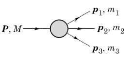
Figure 2: Feynman diagram of the three body decay.

Using the notation of Fig.2 and the definition $m_{ij}=m_{i}+m_{j}$ the corresponding expression for the three-body decay width of the process $A\rightarrow B_{1}B_{2}B_{3}$ reads Patrignani et al. (2016):

$$\Gamma_{A\rightarrow B_{1}B_{2}B_{3}} =\frac{S_{A\rightarrow B_{1}B_{2}B_{3}}}{32(2\pi)^{3}M^{3}}\int_{(m_{1}+m_{2})^{2}}^{(M-m_{3})^{2}}|-i\mathcal{M}_{A\rightarrow B_{1}B_{2}B_{3}}|^{2}$$

$$\times\sqrt{\frac{(-m_{1}+m_{12}-m_{2})(m_{1}+m_{12}-m_{2})(-m_{1}+m_{12}+m_{2})(m_{1}+m_{12}+m_{2})}{m_{12}^{2}}}$$

$$\times\sqrt{\frac{(-M+m_{12}-m_{3})(M+m_{12}-m_{3})(-M+m_{12}+m_{3})(M+m_{12}+m_{3})}{m_{12}^{2}}}dm_{12}^{2}\text{ ,}$$ (25)

where $\mathcal{M}_{A\rightarrow B_{1}B_{2}B_{3}}$ is the corresponding tree-level decay amplitude, and $S_{A\rightarrow B_{1}B_{2}B_{3}}$ is a symmetrization factor (equal to $1$ if the $B_{i}$ are all different, equal to $2$ for two identical particles in the final state, and equal to $6$ for three identical particles).

Appendix B Decay rates for $\chi_{c0}$

We present the explicit expressions for the two- and three-body decay rates for the scalar hidden-charmed meson $\chi_{c0}$.

B.1 Two-body decay rates for $\chi_{C0}$

The explicit expressions for the two-body decay rates of $\chi_{c0}$ are extracted from the Lagrangian (1) and are presented in the following.

Decay channel $\chi_{C0}\rightarrow\overline{K}^{\ast 0}_{0}K^{\ast 0}_{0}$

The corresponding interaction part of the Lagrangian (1) reads

$$\mathcal{L}_{\chi_{C0}\overline{K}^{\ast}_{0}K^{\ast}_{0}}= -2\lambda_{1}^{C}\,Z_{K^{\ast}_{0}}^{2}\,\phi_{C}\,\chi_{C0}(\overline{K}^{\ast 0}_{0}K^{\ast 0}_{0}+K^{\ast-}_{0}K^{\ast+}_{0})$$

$$-h_{1}^{C}\,\phi_{C}\,Z_{K^{\ast}_{0}}^{2}\omega^{2}_{K^{\ast}}\chi_{C0}(\partial_{\mu}K^{\ast 0}_{0}\partial^{\mu}\overline{K}^{\ast 0}_{0}+\partial_{\mu}K^{\ast-}_{0}\partial^{\mu}K^{\ast+}_{0})\,.$$ (26)

Consider only the $\chi_{C0}\rightarrow\overline{K}^{\ast 0}_{0}K^{\ast 0}_{0}$ decay channel, the $\chi_{C0}\rightarrow K^{\ast-}_{0}K^{\ast+}_{0}$ will give the same contribution due to isospin symmetry,

$$\mathcal{L}_{\chi_{C0}\overline{K}^{\ast 0}_{0}K^{\ast 0}_{0}}= -2\lambda_{1}^{C}\,Z_{K^{\ast}_{0}}^{2}\,\phi_{C}\,\chi_{C0}\overline{K}^{\ast 0}_{0}K^{\ast 0}_{0}-h_{1}^{C}\,\phi_{C}\,Z_{K^{\ast}_{0}}^{2}\omega^{2}_{K^{\ast}}\chi_{C0}\partial_{\mu}K^{\ast 0}_{0}\partial^{\mu}\overline{K}^{\ast 0}_{0}\,.$$ (27)

Let us denote the momenta of ${K}^{\ast 0}_{0}$ and $\overline{K}^{\ast 0}_{0}$ as $P_{1}$ and $P_{2}$, respectively. The energy-momentum conservation on the vertex implies $P=P_{1}+P_{2}$, where $P$ denotes the momenta of the decaying particle $\chi_{C0}$. Given that our particles are on-shell, we obtain

$$P_{1}\cdot P_{2}=\frac{P^{2}-P_{1}^{2}-P_{2}^{2}}{2}=\frac{m_{\chi_{C0}}^{2}-2\,m_{K^{\ast 0}_{0}}}{2}\,.$$ (28)

Upon substituting $\partial_{\mu}\rightarrow-iP^{\mu}$ for the decay particle and $\partial_{\mu}\rightarrow+iP_{1,2}^{\mu}$ for the outgoing particles, one obtains

$$\mathcal{L}_{\chi_{C0}\overline{K}^{\ast 0}_{0}K^{\ast 0}_{0}}=\phi_{C}\,Z_{K^{\ast}_{0}}^{2}\bigg{[}-2\lambda_{1}^{C}+h_{1}^{C}\omega^{2}_{K^{\ast}}\frac{m_{\chi_{c0}}^{2}-2m_{K^{\ast}_{0}}^{2}}{2}\bigg{]}\chi_{C0}K^{\ast 0}_{0}\overline{K}^{\ast 0}_{0}\,.$$ (29)

Consequently, the decay amplitude is given by

$$-i\mathcal{M}_{\chi_{C0}\rightarrow\overline{K}^{\ast 0}_{0}K^{\ast 0}_{0}}=i\phi_{C}\,Z_{K^{\ast}_{0}}^{2}\bigg{[}2\lambda_{1}^{C}-h_{1}^{C}\omega^{2}_{K^{\ast}}\frac{m_{\chi_{c0}}^{2}-2m_{K^{\ast}_{0}}^{2}}{2}\bigg{]}\,.$$ (30)

The decay width is obtained as

$$\Gamma_{\chi_{C0}\rightarrow\overline{K}^{\ast 0}_{0}K^{\ast 0}_{0}}=\frac{|\overrightarrow{k}_{1}|}{8\pi\,m_{\chi_{C0}}^{2}}|-i\mathcal{M}_{\chi_{C0}\rightarrow\overline{K}^{\ast 0}_{0}K^{\ast 0}_{0}}|^{2}\,.$$ (31)

Decay channel $\chi_{C0}\rightarrow K^{-}K^{+}$

The corresponding interaction part of the Lagrangian (1) reads

$$\mathcal{L}_{\chi_{C0}KK}= -2\lambda_{1}^{C}\,Z_{K}^{2}\,\phi_{C}\,\chi_{C0}(\overline{K}^{0}K^{0}+K^{-}K^{+}_{0})$$

$$+h_{1}^{C}\,\phi_{C}\,Z_{K}^{2}\omega^{2}_{K_{1}}\chi_{C0}(\partial_{\mu}K^{0}\partial^{\mu}\overline{K}^{0}+\partial_{\mu}K^{-}\partial^{\mu}K^{+})\,.$$ (32)

In a similar way as the previous case, one can obtain the decay width for the channel $\chi_{C0}\rightarrow K^{-}K^{+}$ as

$$\Gamma_{\chi_{C0}\rightarrow K^{-}K^{+}}=\frac{|\overrightarrow{k}_{1}|}{8\pi\,m_{\chi_{C0}}^{2}}\,\phi_{C}^{2}\,Z_{K}^{4}\bigg{[}2\lambda_{1}^{C}+h_{1}^{C}\omega^{2}_{K_{1}}\bigg{(}\frac{m_{\chi_{c0}}^{2}-2m_{K}^{2}}{2}\bigg{)}\bigg{]}^{2}\,.$$ (33)

Decay channel $\chi_{C0}\rightarrow\pi\pi$

The corresponding interaction part of the Lagrangian (1) reads

$$\mathcal{L}_{\chi_{C0}\pi\pi}=-\lambda_{1}^{C}\,\phi_{C}\,Z_{\pi}^{2}\,\chi_{C0}({\pi^{0}}^{2}+2\pi^{-}\pi^{+})+\frac{1}{2}h_{1}^{C}\,\phi_{C}\,Z_{\pi}^{2}\omega^{2}_{a_{1}}\chi_{C0}[(\partial_{\mu}\pi^{0})^{2}+2\partial_{\mu}\pi^{-}\partial^{\mu}\pi^{+}]\,,$$ (34)

and leads to the decay width

$$\Gamma_{\chi_{C0}\rightarrow\pi\pi}=\frac{3}{2}\frac{|\overrightarrow{k}_{1}|}{8\pi\,m_{\chi_{C0}}^{2}}\,\phi_{C}^{2}\,Z_{\pi}^{4}\bigg{[}2\lambda_{1}^{C}+h_{1}^{C}\omega^{2}_{a_{1}}\bigg{(}\frac{m_{\chi_{c0}}^{2}-2m_{\pi}^{2}}{2}\bigg{)}\bigg{]}^{2}\,.$$ (35)

Decay channel $\chi_{C0}\rightarrow\overline{K}^{\ast 0}K^{\ast 0}$

The corresponding interaction Lagrangian is extracted as

$$\mathcal{L}_{\chi_{C0}\overline{K}^{\ast 0}K^{\ast 0}}=h_{1}^{C}\,\phi_{C}\,\chi_{C0}(K^{\ast-}_{\mu}K^{\ast+\mu}+K^{\ast 0}_{\mu}\overline{K}^{\ast 0\mu})\,.$$ (36)

Consider only the $K^{\ast 0}_{\mu}\overline{K}^{\ast 0\mu}$ decay channel, then

$$\mathcal{L}_{\chi_{C0}\overline{K}^{\ast 0}K^{\ast 0}}=h_{1}^{C}\,\phi_{C}\,\chi_{C0}K^{\ast 0}_{\mu}\overline{K}^{\ast 0\mu}\,.$$ (37)

Put

$$A_{\chi_{C0}\overline{K}^{\ast 0}K^{\ast 0}}=h_{1}^{C}\,\phi_{C}\,.$$ (38)

Let us denote the momenta of $\chi_{C0}$, $\overline{K}^{\ast 0}$, and $K^{\ast 0}$ as $P$, $P_{1}$, and $P_{2}$, respectively, while the polarisation vectors are denoted as $\varepsilon_{\mu}^{(\alpha)}(P_{1})$ and $\varepsilon_{\nu}^{(\beta)}(P_{2})$. Then, upon substituting $\partial^{\mu}\rightarrow iP_{1,2}^{\mu}$ for the outgoing particles, we obtain the following Lorentz-invariant $\chi_{C0}\overline{K}^{\ast 0}K^{\ast 0}$ scattering amplitude $-i\mathcal{M}^{(\alpha,\beta)}_{\chi_{C0}\rightarrow\overline{K}^{\ast 0}K^{\ast 0}}$:

$$-i\mathcal{M}_{\chi_{C0}\rightarrow\overline{K}^{\ast 0}K^{\ast 0}}^{(\alpha,\beta)}=\varepsilon_{\mu}^{(\alpha)}(P_{1})\varepsilon_{\nu}^{(\beta)}(P_{2})h_{\chi_{C0}\overline{K}^{\ast 0}K^{\ast 0}}^{\mu\nu}\,,$$ (39)

with

$$h_{\chi_{C0}\overline{K}^{\ast 0}K^{\ast 0}}^{\mu\nu}=iA_{\chi_{C0}\overline{K}^{\ast 0}K^{\ast 0}}g^{\mu\nu}\text{,}$$ (40)

where $h_{\chi_{C0}\overline{K}^{\ast 0}K^{\ast 0}}^{\mu\nu}$ denotes the $\chi_{C0}\overline{K}^{\ast 0}K^{\ast 0}$ vertex.

The averaged squared amplitude $|\overline{-i\mathcal{M}}|^{2}$ is determined as follows:

$$\left|\overline{-i\mathcal{M}_{\chi_{C0}\rightarrow\overline{K}^{\ast 0}K^{\ast 0}}}\right|^{2}= \frac{1}{3}\sum\limits_{\alpha,\beta=1}^{3}\left|-i\mathcal{M}_{\chi_{C0}\rightarrow\overline{K}^{\ast 0}K^{\ast 0}}^{(\alpha,\beta)}\right|^{2}$$

$$= \frac{1}{3}\sum\limits_{\alpha,\beta=1}^{3}\varepsilon_{\mu}^{(\alpha)}(P_{1})\varepsilon_{\nu}^{(\beta)}(P_{2})h_{\chi_{C0}\overline{K}^{\ast 0}K^{\ast 0}}^{\mu\nu}\varepsilon_{\kappa}^{(\alpha)}(P_{1})$$

$$\,\,\,\,\,\,\,\,\,\,\,\,\,\,\,\,\,\,\,\,\,\times\varepsilon_{\lambda}^{(\beta)}(P_{2})h_{\chi_{C0}\overline{K}^{\ast 0}K^{\ast 0}}^{\ast\kappa\lambda}\text{ .}$$ (41)

Then,

$$|\overline{-i\mathcal{M}_{\chi_{C0}\rightarrow\overline{K}^{\ast 0}K^{\ast 0}}}|^{2}=\frac{1}{3}\bigg{[}\left|h_{\chi_{C0}\overline{K}^{\ast 0}K^{\ast 0}}^{\mu\nu}\right|^{2} -\frac{\left|h_{\chi_{C0}\overline{K}^{\ast 0}K^{\ast 0}}^{\mu\nu}P_{1\mu}\right|^{2}}{m_{V_{1}}^{2}}-\frac{\left|h_{\chi_{C0}\overline{K}^{\ast 0}K^{\ast 0}}^{\mu\nu}P_{2\nu}\right|^{2}}{m_{V_{2}}^{2}}$$

$$+\frac{\left|h_{\chi_{C0}\overline{K}^{\ast 0}K^{\ast 0}}^{\mu\nu}P_{1\mu}P_{2\nu}\right|^{2}}{m_{V_{1}}^{2}m_{V_{2}}^{2}}\bigg{]}\text{ .}$$ (42)

From Eq. (40) we obtain

$$h_{\chi_{C0}\overline{K}^{\ast 0}K^{\ast 0}}^{\mu\nu}P_{1\mu}=iA_{\chi_{C0}\overline{K}^{\ast 0}K^{\ast 0}}P_{1}^{\nu}\,,$$

$$h_{\chi_{C0}\overline{K}^{\ast 0}K^{\ast 0}}^{\mu\nu}P_{2\nu}=iA_{\chi_{C0}\overline{K}^{\ast 0}K^{\ast 0}}P_{2}^{\mu}\,,$$

and

$$h_{\chi_{C0}\overline{K}^{\ast 0}K^{\ast 0}}^{\mu\nu}P_{1\mu}P_{2\nu}=iA_{\chi_{C0}\overline{K}^{\ast 0}K^{\ast 0}}P_{1}\cdot P_{2}\,,$$

and consequently

$$|\overline{-i\mathcal{M}_{\chi_{C0}\rightarrow\overline{K}^{\ast 0}K^{\ast 0}}}|^{2}=\frac{1}{3}\left[4-\frac{P_{1}^{2}}{m_{K^{\ast 0}}^{2}}-\frac{P_{2}^{2}}{m_{\overline{K}^{\ast 0}}^{2}}+\frac{(P_{1}\cdot P_{2})^{2}}{m_{K^{\ast 0}}^{2}m_{\overline{K}^{\ast 0}}^{2}}\right]A_{\chi_{C0}\overline{K}^{\ast 0}K^{\ast 0}}^{2}\text{.}$$ (43)

For on-shell states, $P_{1,2}^{2}=m_{\overline{K}^{\ast 0},K^{\ast 0}}^{2}$ and Eq. (43) reduces to

$$|\overline{-i\mathcal{M}_{\chi_{C0}\rightarrow\overline{K}^{\ast 0}K^{\ast 0}}}|^{2} =\frac{1}{3}\left[2+\frac{(P_{1}\cdot P_{2})^{2}}{m_{\overline{K}^{\ast 0}}^{2}m_{K^{\ast 0}}^{2}}\right]A_{\chi_{C0}\overline{K}^{\ast 0}K^{\ast 0}}^{2}$$

$$=\frac{1}{3}\left[2+\frac{(m_{\chi_{C0}}^{2}-m_{\overline{K}^{\ast 0}}^{2}-m_{K^{\ast 0}}^{2})^{2}}{4m_{\overline{K}^{\ast 0}}^{2}m_{K^{\ast 0}}^{2}}\right]A_{\chi_{C0}\overline{K}^{\ast 0}K^{\ast 0}}^{2}\text{.}$$ (44)

Consequently, the decay width is

$$\Gamma_{\chi_{C0}\rightarrow\overline{K}^{\ast 0}K^{\ast 0}}=\frac{|\overrightarrow{k}_{1}|}{8\pi m_{\chi_{C0}}^{2}}|\overline{-i\mathcal{M}_{\chi_{C0}\rightarrow\overline{K}^{\ast 0}K^{\ast 0}}}|^{2}\,.$$ (45)

Decay channel $\chi_{C0}\rightarrow\omega\omega$

The corresponding interaction Lagrangian is extracted as

$$\mathcal{L}_{\chi_{C0}\omega\omega}=\frac{1}{2}h_{1}^{C}\,\phi_{C}\,\chi_{C0}\omega_{N}^{\mu}\omega_{N\mu}\,,$$ (46)

which also has the same form as the interaction Lagrangian $\mathcal{L}_{\chi_{C0}\rightarrow\overline{K}^{\ast 0}K^{\ast 0}}$. Thus one can obtain the decay width of $\chi_{C0}\rightarrow\omega\omega$ as

$$\Gamma_{\chi_{C0}\rightarrow\omega\omega}=2\frac{[m_{\chi_{C0}}^{4}-4m_{\omega}^{2}m_{\chi_{C0}}^{2}]^{1/2}}{16\pi m_{\chi_{C0}}^{3}}\,\,\frac{1}{4}(h_{1}^{C})^{2}\,\phi_{C}^{2}\bigg{[}2+\frac{(m_{\chi_{C0}}^{2}-2m_{\omega}^{2})^{2}}{4m_{\omega}^{4}}\bigg{]}\,.$$ (47)

Decay channel $\chi_{C0}\rightarrow\phi\phi$

The corresponding interaction Lagrangian is extracted as

$$\mathcal{L}_{\chi_{C0}\omega\omega}=\frac{1}{2}h_{1}^{C}\,\phi_{C}\,\chi_{C0}\omega_{S}^{\mu}\omega_{S\mu}\,.$$ (48)

Similar to the decay width for $\chi_{C0}\rightarrow\omega\omega$, the decay width for $\chi_{C0}\rightarrow\phi\phi$ is

$$\Gamma_{\chi_{C0}\rightarrow\phi\phi}=2\frac{[m_{\chi_{C0}}^{4}-4m_{\phi}^{2}m_{\chi_{C0}}^{2}]^{1/2}}{16\pi m_{\chi_{C0}}^{3}}\,\,\frac{1}{4}(h_{1}^{C})^{2}\,\phi_{C}^{2}\bigg{[}2+\frac{(m_{\chi_{C0}}^{2}-2m_{\phi}^{2})^{2}}{4m_{\phi}^{4}}\bigg{]}\,.$$ (49)

Decay channel $\chi_{C0}\rightarrow\rho\rho$

The corresponding interaction Lagrangian is extracted as

$$\mathcal{L}_{\chi_{C0}\rho\rho}=\frac{1}{2}h_{1}^{C}\,\phi_{C}\,\chi_{C0}(\rho^{0\mu}\rho^{0}_{\mu}+2\rho^{-\mu}\rho^{+}_{\mu})\,,$$ (50)

which also has the same form as $\mathcal{L}_{\chi_{C0}\omega\omega}$. We thus obtain the decay width as

$$\Gamma_{\chi_{C0}\rightarrow\rho\rho} =3\Gamma_{\chi_{C0}\rightarrow\rho^{0}\rho^{0}}$$

$$=3\frac{[m_{\chi_{C0}}^{4}-4m_{\rho^{0}}^{2}m_{\chi_{C0}}^{2}]^{1/2}}{16\pi m_{\chi_{C0}}^{3}}\times\frac{1}{12}(h_{1}^{C})^{2}\,\phi_{C}^{2}\bigg{[}2+\frac{(m_{\chi_{C0}}^{2}-2m_{\rho^{0}}^{2})^{2}}{4m_{\rho^{0}}^{4}}\bigg{]}\,.$$ (51)

Decay channel $\chi_{C0}\rightarrow a_{0}a_{0}$

The corresponding interaction Lagrangian has the form

$$\mathcal{L}_{\chi_{C0}a_{0}a_{0}}= -\lambda_{1}^{C}\,\phi_{C}\,\chi_{C0}({a_{0}^{0}}^{2}+2a_{0}^{-}\,a_{0}^{+})\,.$$ (52)

The decay width of $\chi_{C0}$ into $a_{0}a_{0}$ can be obtained as

$$\Gamma_{\chi_{C0}\rightarrow a_{0}\,a_{0}} =3\Gamma_{\chi_{C0}\rightarrow a^{0}_{0}\,a^{0}_{0}}$$

$$=3\frac{(\lambda_{1}^{C})^{2}\,\phi_{C}^{2}}{8\pi\,m_{\chi_{C0}}^{2}}\,\,\frac{[m_{\chi_{C0}}^{4}-4m_{a_{0}^{0}}^{2}\,m_{\chi_{C0}}^{2}]^{1/2}}{2m_{\chi_{C0}}}\,.$$ (53)

Decay channel $\chi_{C0}\rightarrow K^{\ast}\overline{K}^{\ast}_{0}$

The corresponding interaction Lagrangian from the Lagrangian (1) reads

$$\mathcal{L}_{\chi_{C0}K^{\ast 0}\overline{K}^{\ast 0}_{0}}=Z_{K_{0}^{\ast}}\,w_{K^{\ast}}\,h_{1}^{C}\,\phi_{C}\,\chi_{C0}\overline{K}^{\ast 0\mu}_{0}\partial_{\mu}K^{\ast 0}_{0}\,,$$ (54)

which obtain from the corresponding interaction Lagrangian

$$\mathcal{L}_{\chi_{C0}K^{\ast}\overline{K}^{\ast}_{0}}=Z_{K_{0}^{\ast}}\,w_{K^{\ast}}\,h_{1}^{C}\,\phi_{C}\,\chi_{C0}(\overline{K}^{\ast 0\mu}_{0}\partial_{\mu}K^{\ast 0}_{0}-\partial_{\mu}K^{\ast-}_{0}K^{\ast+\mu}+\partial_{\mu}K^{\ast+}_{0}K^{\ast-\mu}-\partial_{\mu}\overline{K}^{\ast 0\mu}_{0}K^{\ast 0\mu})\,.$$ (55)

We compute the decay width as

$$\Gamma_{\chi_{C0}\rightarrow K^{\ast 0}\overline{K}^{\ast 0}_{0}}=\frac{|\overrightarrow{k}_{1}|}{8\pi\,m_{\chi_{C0}}^{2}}w_{K^{\ast}}^{2}\,Z_{K^{\ast}}(h_{1}^{C})^{2}\phi_{C}^{2}\left|-m_{K^{\ast 0}}^{2}+\frac{(m_{\chi_{C0}}^{2}-m_{K^{\ast 0}}^{2}-m^{2}_{\overline{K}^{\ast 0}_{0}})^{2}}{4m^{2}_{\overline{K}^{\ast 0}_{0}}}\right|\,.$$ (56)

Note that we considered only the decay channel $\chi_{C0}K^{\ast 0}\overline{K}^{\ast 0}_{0}$ because the other decay channels contribute the same of isospin symmetry reasons. Thus,

$$\Gamma_{\chi_{C0}\rightarrow K^{\ast}\overline{K}^{\ast}_{0}}=\Gamma_{\chi_{C0}\rightarrow K^{\ast 0}\overline{K}^{\ast 0}_{0}}+\Gamma_{\chi_{C0}\rightarrow K^{\ast+}K^{\ast-}_{0}}+\Gamma_{\chi_{C0}\rightarrow K^{\ast-}K^{\ast+}_{0}}+\Gamma_{\chi_{C0}\rightarrow K^{\ast 0}_{0}\overline{K}^{\ast 0}}\,.$$ (57)

Decay channels $\chi_{C0}\rightarrow\eta,\,\eta^{\prime}$

The corresponding interaction Lagrangian of $\chi_{C0}$ with the $\eta^{\prime}$ and the $\eta$ resonances reads

$$\mathcal{L}_{\chi_{C0}\eta_{N}\eta_{N},\eta_{S}\eta_{S},\eta_{N}\eta_{S}}= (-\lambda_{1}^{C}-\frac{1}{2}c\phi_{N}^{2}\phi_{S}^{2})Z^{2}_{\eta_{N}}\,\phi_{C}\,\chi_{C0}\eta_{N}^{2}+\frac{1}{2}h_{1}^{C}\,w_{f_{1N}}^{2}\,Z_{\eta_{N}}^{2}\chi_{C0}\,\partial_{\mu}\eta_{N}\partial^{\mu}\eta_{N}$$

$$+(-\lambda_{1}^{C}-\frac{1}{8}c\phi_{N}^{4})Z^{2}_{\eta_{S}}\,\phi_{C}\,\chi_{C0}\eta_{S}^{2}+\frac{1}{2}h_{1}^{C}\,w_{f_{1S}}^{2}Z_{\eta_{S}}^{2}\chi_{C0}\partial_{\mu}\eta_{S}\partial^{\mu}\eta_{S}$$

$$-\frac{1}{2}\phi_{N}^{3}\phi_{C}\phi_{S}\,Z_{\eta_{N}}\,Z_{\eta_{S}}\,\eta_{N}\eta_{S}\,.$$ (58)

By using Eq. (11), the interaction Lagrangian (58) will transform to a Lagrangian which describes the interaction of $\chi_{C0}$ with $\eta$ and $\eta^{\prime}$,

$$\mathcal{L}_{\chi_{C0}\eta^{2},\eta^{\prime 2},\eta\eta^{\prime}} =[-\lambda_{1}^{C}(Z^{2}_{\eta_{N}}\cos^{2}\varphi_{\eta}+Z^{2}_{\eta_{S}}\sin^{2}\varphi_{\eta})-\frac{1}{2}c\phi_{N}^{2}(\phi_{S}^{2}\,Z^{2}_{\eta_{N}}\,\cos^{2}\varphi_{\eta}$$

$$+\frac{1}{4}\phi_{N}^{2}Z^{2}_{\eta_{S}}\sin^{2}\varphi_{\eta}+\phi_{N}\phi_{S}\,Z_{\eta_{N}}Z_{\eta_{S}}\sin\varphi_{\eta}\cos\varphi_{\eta})]\phi_{C}\chi_{C0}\eta^{2}$$

$$+\bigg{[}\frac{1}{2}h_{1}^{C}\phi_{C}(w^{2}_{f_{1N}}Z_{\eta_{N}}^{2}\cos^{2}\varphi_{\eta}+w^{2}_{f_{1S}}Z_{\eta_{S}}^{2}\sin^{2}\varphi_{\eta})\bigg{]}\chi_{C0}\partial_{\mu}\eta\partial^{\mu}\eta$$

$$[-\lambda_{1}^{C}(Z^{2}_{\eta_{N}}\sin^{2}\varphi_{\eta}+Z^{2}_{\eta_{S}}\cos^{2}\varphi_{\eta})-\frac{1}{2}c\phi_{N}^{2}(\phi_{S}^{2}\,Z^{2}_{\eta_{N}}\,\sin^{2}\varphi_{\eta}$$

$$+\frac{1}{4}\phi_{N}^{2}Z^{2}_{\eta_{S}}\cos^{2}\varphi_{\eta}-\phi_{N}\phi_{S}\,Z_{\eta_{N}}Z_{\eta_{S}}\sin\varphi_{\eta}\cos\varphi_{\eta})]\phi_{C}\chi_{C0}\eta^{\prime 2}$$

$$+\bigg{[}\frac{1}{2}h_{1}^{C}\phi_{C}(w^{2}_{f_{1N}}Z_{\eta_{N}}^{2}\sin^{2}\varphi_{\eta}+w^{2}_{f_{1S}}Z_{\eta_{S}}^{2}\cos^{2}\varphi_{\eta})\bigg{]}\chi_{C0}\partial_{\mu}\eta^{\prime}\partial^{\mu}\eta^{\prime}$$

$$+[-2\lambda_{1}^{C}(-Z^{2}_{\eta_{N}}+Z^{2}_{\eta_{S}})\sin\varphi_{\eta}\cos\varphi_{\eta})$$

$$+\frac{1}{2}c\phi_{N}^{2}(2\phi_{S}^{2}\,Z^{2}_{\eta_{N}}-\frac{1}{2}\phi_{N}^{2}\,Z_{\eta_{S}}^{2})\cos\varphi_{\eta}\sin\varphi_{\eta})$$

$$-\frac{1}{2}c\phi_{N}^{3}\phi_{S}\,Z_{\eta_{N}}Z_{\eta_{S}}(\cos^{2}\varphi_{\eta}-\sin^{2}\varphi_{\eta}\cos\varphi_{\eta})]\phi_{C}\chi_{C0}\eta\eta^{\prime}$$

$$+h_{1}^{C}\phi_{C}\,\cos\varphi_{\eta}\sin\varphi_{\eta}(w^{2}_{f_{1S}}Z_{\eta_{S}}^{2}-w^{2}_{f_{1N}}Z_{\eta_{N}}^{2})\chi_{C0}\partial_{\mu}\eta\partial^{\mu}\eta^{\prime}\,,$$ (59)

which contains three different decay channels, $\chi_{C0}\rightarrow\eta\eta$, $\chi_{C0}\rightarrow\eta^{\prime}\eta^{\prime}$, and $\chi_{C0}\rightarrow\eta\eta^{\prime}$, with the following vertices

$$A_{\chi_{C0}\eta\eta}= -\lambda_{1}^{C}\phi_{C}(Z^{2}_{\eta_{N}}\cos^{2}\varphi_{\eta}+Z^{2}_{\eta_{S}}\sin^{2}\varphi_{\eta})$$

$$-\frac{1}{2}c\phi_{N}^{2}\phi_{C}(\phi_{S}^{2}\,Z^{2}_{\eta_{N}}\,\cos^{2}\varphi_{\eta}+\frac{1}{4}\phi_{N}^{2}Z^{2}_{\eta_{S}}\sin^{2}\varphi_{\eta}+\phi_{N}\phi_{S}\,Z_{\eta_{N}}Z_{\eta_{S}}\sin\varphi_{\eta}\cos\varphi_{\eta})\,,$$ (60)

$$B_{\chi_{C0}\eta\eta} =\frac{1}{2}h_{1}^{C}\phi_{C}(w^{2}_{f_{1N}}Z_{\eta_{N}}^{2}\cos^{2}\varphi_{\eta}+w^{2}_{f_{1S}}Z_{\eta_{S}}^{2}\sin^{2}\varphi_{\eta})\,,$$ (61)

$$A_{\chi_{C0}\eta^{\prime}\eta^{\prime}}= -\lambda_{1}^{C}\phi_{C}(Z^{2}_{\eta_{N}}\sin^{2}\varphi_{\eta}+Z^{2}_{\eta_{S}}\cos^{2}\varphi_{\eta})$$

$$-\frac{1}{2}c\phi_{N}^{2}\phi_{C}(\phi_{S}^{2}\,Z^{2}_{\eta_{N}}\,\sin^{2}\varphi_{\eta}+\frac{1}{4}\phi_{N}^{2}Z^{2}_{\eta_{S}}\cos^{2}\varphi_{\eta}-\phi_{N}\phi_{S}\,Z_{\eta_{N}}Z_{\eta_{S}}\sin\varphi_{\eta}\cos\varphi_{\eta})\,,$$ (62)

$$B_{\chi_{C0}\eta^{\prime}\eta^{\prime}} =\frac{1}{2}h_{1}^{C}\phi_{C}(w^{2}_{f_{1N}}Z_{\eta_{N}}^{2}\sin^{2}\varphi_{\eta}+w^{2}_{f_{1S}}Z_{\eta_{S}}^{2}\cos^{2}\varphi_{\eta})\,,$$ (63)

$$A_{\chi_{C0}\eta\eta^{\prime}}= -2\lambda_{1}^{C}\phi_{C}(-Z^{2}_{\eta_{N}}+Z^{2}_{\eta_{S}})\sin\varphi_{\eta}\cos\varphi_{\eta}+\frac{1}{2}c\phi_{N}^{2}\phi_{C}(2\phi_{S}^{2}\,Z^{2}_{\eta_{N}}-\frac{1}{2}\phi_{N}^{2}\,Z_{\eta_{S}}^{2})\cos\varphi_{\eta}\sin\varphi_{\eta}$$

$$-\frac{1}{2}c\phi_{N}^{3}\phi_{S}\phi_{C}\,Z_{\eta_{N}}Z_{\eta_{S}}(\cos^{2}\varphi_{\eta}-\sin^{2}\varphi_{\eta}\cos\varphi_{\eta})\,,$$ (64)

$$B_{\chi_{C0}\eta\eta^{\prime}} =h_{1}^{C}\phi_{C}\,\cos\varphi_{\eta}\sin\varphi_{\eta}(w^{2}_{f_{1S}}Z_{\eta_{S}}^{2}-w^{2}_{f_{1N}}Z_{\eta_{N}}^{2})\,.$$ (65)

Let us firstly consider the channel $\chi_{C0}\rightarrow\eta\eta$. We denote the momenta of the two outgoing $\eta$ particles as $P_{1}$ and $P_{2}$, and $P$ denotes the momentum of the decaying $\chi_{C0}$ particle. Given that our particles are on shell, we obtain

$$P_{1}\cdot P_{2}=\frac{P^{2}-P_{1}^{2}-P_{2}^{2}}{2}=\frac{m_{\chi_{C0}}^{2}-2m_{\eta}^{2}}{2}\,.$$ (66)

After replacing $\partial_{\mu}\rightarrow+iP^{\mu}$ for the outgoing particles, one obtains the decay amplitude as

$$-iM_{\chi_{C0}\rightarrow\eta\eta}=i\bigg{[}A_{\chi_{C0}\eta\eta}-B_{\chi_{C0}\eta\eta}\frac{m_{\chi_{C0}}^{2}-2m_{\eta}^{2}}{2}\bigg{]}\,.$$ (67)

Then the decay width is

$$\Gamma_{\chi_{C0}\rightarrow\eta\eta}=2\frac{|\overrightarrow{k}_{1}|}{8\pi\,m_{\chi_{C0}}^{2}}\left|\overline{-i\mathcal{M}_{\chi_{C0}\rightarrow\eta\eta}}\right|^{2}\,.$$ (68)

Similarly, the decay width of $\chi_{C0}$ into $\eta^{\prime}\eta^{\prime}$ is obtained as

$$\Gamma_{\chi_{C0}\rightarrow\eta^{\prime}\eta^{\prime}}=2\frac{|\overrightarrow{k}_{1}|}{8\pi\,m_{\chi_{C0}}^{2}}\left|A_{\chi_{C0}\eta^{\prime}\eta^{\prime}}-B_{\chi_{C0}\eta^{\prime}\eta^{\prime}}\frac{m_{\chi_{C0}}^{2}-2m_{\eta^{\prime}}^{2}}{2}\right|^{2}\,.$$ (69)

In a similar way, the decay width of $\chi_{C0}$ into $\eta\eta^{\prime}$ can be obtained as

$$\Gamma_{\chi_{C0}\rightarrow\eta\eta^{\prime}}=\frac{|\overrightarrow{k}_{1}|}{8\pi\,m_{\chi_{C0}}^{2}}\left|A_{\chi_{C0}\eta\eta^{\prime}}-B_{\chi_{C0}\eta\eta^{\prime}}\frac{m_{\chi_{C0}}^{2}-m_{\eta}^{2}-m_{\eta^{\prime}}^{2}}{2}\right|^{2}\,.$$ (70)

Decay channels $\chi_{C0}\rightarrow f_{0}f_{0}$

The corresponding interaction Lagrangian is extracted from the Lagrangian (1)

$$\mathcal{L}_{\chi_{C0}f_{0}f_{0}}=-\lambda_{1}^{C}\,\phi_{C}\,\chi_{C0}(\sigma_{N}^{2}+\sigma_{S}^{2})-\frac{m_{0}^{2}}{G_{0}^{2}}\,\phi_{C}\,\chi_{C0}\,G^{2}\,.$$ (71)

By using the mixing matrices (14), (15) and (16), we obtain the interaction Lagrangian (71) as a function of all the following channels:

$$\chi_{C0}\rightarrow f_{0}(1370)f_{0}(1370),\,\chi_{C0}\rightarrow f_{0}(1500)f_{0}(1500),$$

$$\chi_{C0}\rightarrow f_{0}(1370)f_{0}(1500),\,\,\chi_{C0}\rightarrow f_{0}(1370)f_{0}(1710),$$

$$\chi_{C0}\rightarrow f_{0}(1500)f_{0}(1710),\,\,$$

Then, we compute the decay widths for all these channels by using the formula of the two-body decay (23).

B.2 Three-body decay rates for $\chi_{C0}$

Decay channel $\chi_{C0}\rightarrow K^{\ast}_{0}K\eta,\eta^{\prime}$

The corresponding interaction Lagrangian can be obtained from the Lagrangian (1) as

$$\mathcal{L}_{\chi_{C0}K^{\ast}_{0}K\eta_{N},\eta_{S}}= \frac{1}{\sqrt{2}}(c-\frac{1}{2}\phi_{C}^{2}\delta\widetilde{c})Z_{K}\,Z_{K^{\ast}_{0}}\,Z_{\eta_{N}}\phi_{N}^{2}\phi_{S}\phi_{C}\chi_{C0}\eta_{N}(K^{\ast 0}_{0}\overline{K}^{0}+\overline{K}^{\ast 0}_{0}K^{0}+K^{\ast-}_{0}K^{+}+K^{\ast+}_{0}K^{-})$$

$$+\frac{\sqrt{2}}{4}(c-\frac{1}{2}\phi_{C}^{2}\delta\widetilde{c})Z_{K}\,Z_{K^{\ast}_{0}}\,Z_{\eta_{S}}\phi_{N}^{3}\phi_{C}\chi_{C0}\eta_{S}(K^{\ast 0}_{0}\overline{K}^{0}+\overline{K}^{\ast 0}_{0}K^{0}+K^{\ast-}_{0}K^{+}+K^{\ast+}_{0}K^{-})\,.$$ (72)

Using Eq. (11), the interaction Lagrangian (72) can be written as

$$\mathcal{L}_{\chi_{C0}K^{\ast}_{0}K\eta,\eta^{\prime}}=\frac{1}{\sqrt{2}}(c-\frac{1}{2}\phi_{C}^{2}\delta\widetilde{c})\phi_{C}\phi_{N}^{2}Z_{K}Z_{K^{\ast}_{0}}\chi_{co}\bigg{[} (\phi_{S}Z_{\eta_{N}}\cos\varphi_{\eta}+\frac{1}{2}\phi_{N}Z_{\eta_{S}}\sin\varphi_{\eta})\eta$$

$$-(\phi_{S}Z_{\eta_{N}}\sin\varphi_{\eta}-\frac{1}{2}\phi_{N}Z_{\eta_{S}}\cos\varphi_{\eta})\eta^{\prime}\bigg{]}$$

$$\times\big{[}K^{\ast 0}_{0}\overline{K}^{0}+\overline{K}^{\ast 0}_{0}K^{0}+K^{\ast-}_{0}K^{+}+K^{\ast+}_{0}K^{-}\big{]}\,.$$ (73)

Consequently, the amplitude decay for the decay channels $\chi_{C0}\rightarrow K^{\ast}_{0}K\eta$ and $\chi_{C0}\rightarrow K^{\ast}_{0}K\eta^{\prime}$ can be obtain as

$$-i\mathcal{M}_{\chi_{C0}\rightarrow K^{\ast}_{0}K\eta}=-i\frac{1}{\sqrt{2}}(c-\frac{1}{2}\phi_{C}^{2}\delta\widetilde{c})\phi_{C}\phi_{N}^{2}Z_{K}Z_{K^{\ast}_{0}}(\phi_{S}Z_{\eta_{N}}\cos\varphi_{\eta}+\frac{1}{2}\phi_{N}Z_{\eta_{S}}\sin\varphi_{\eta})\,,$$ (74)

and

$$-i\mathcal{M}_{\chi_{C0}\rightarrow K^{\ast}_{0}K\eta^{\prime}}=\frac{1}{\sqrt{2}}(c-\frac{1}{2}\phi_{C}^{2}\delta\widetilde{c})\phi_{C}\phi_{N}^{2}Z_{K}Z_{K^{\ast}_{0}}(-\phi_{S}Z_{\eta_{N}}\sin\varphi_{\eta}+\frac{1}{2}\phi_{N}Z_{\eta_{S}}\cos\varphi_{\eta})\,,$$ (75)

which are used to compute $\Gamma_{\chi_{C0}\rightarrow K^{\ast}_{0}K\eta}$ and $\Gamma_{\chi_{C0}\rightarrow K^{\ast}_{0}K\eta^{\prime}}$ by Eq.(25).

Decay channel $\chi_{C0}\rightarrow f_{0}\eta,\eta^{\prime}$

The corresponding interaction Lagrangian is extracted from the Lagrangian (1) and given by

$$\mathcal{L}_{\chi_{C0}\sigma_{N,S}\eta_{NS}}= -\frac{3}{2}(c-\frac{1}{2}\phi_{C}^{2}\delta\widetilde{c})\,Z_{\eta_{N}}Z_{\eta_{S}}\phi_{N}^{2}\phi_{S}\phi_{C}\chi_{C0}\sigma_{N}\eta_{N}\eta_{S}-c\,Z^{2}_{\eta_{N}}\phi_{N}^{2}\phi_{S}\phi_{C}\chi_{C0}\sigma_{S}\eta_{N}^{2}$$

$$-(c-\frac{1}{2}\phi_{C}^{2}\delta\widetilde{c})\,Z^{2}_{\eta_{N}}\phi_{N}^{2}\phi^{2}_{S}\phi_{C}\chi_{C0}\sigma_{N}\eta^{2}_{N}-\frac{1}{2}(c-\frac{1}{2}\phi_{C}^{2}\delta\widetilde{c})\,Z^{2}_{\eta_{S}}\phi_{N}^{3}\phi_{C}\chi_{C0}\sigma_{N}\eta^{2}_{S}$$

$$-\frac{1}{2}(c-\frac{1}{2}\phi_{C}^{2}\delta\widetilde{c})Z_{\eta_{N}},Z_{\eta_{S}}\phi_{N}^{3}\phi_{C}\chi_{C0}\sigma_{S}\eta_{S}\eta_{N}\,.$$ (76)

We get the decay amplitudes for the following channels:

$$\chi_{C0}\rightarrow f_{0}(1370)\eta\eta,\,\,\chi_{C0}\rightarrow f_{0}(1370)\eta^{\prime}\eta^{\prime}$$

$$\chi_{C0}\rightarrow f_{0}(1370)\eta\eta^{\prime},\,\,\chi_{C0}\rightarrow f_{0}(1500)\eta\eta$$

$$\chi_{C0}\rightarrow f_{0}(1500)\eta\eta^{\prime},\,\,\chi_{C0}\rightarrow f_{0}(1710)\eta\eta$$

$$\chi_{C0}\rightarrow f_{0}(1710)\eta\eta^{\prime},\,\,$$

which used in Eq.(25) to compute the decay widths for all these channels.

Appendix C Decay rates for $\eta_{C}$

We present the explicit expressions for the two- and three-body decay rates for the pseudoscalar hidden-charmed meson $\eta_{C}$.

The chiral Lagrangian contains the tree-level vertices for the decay processes of the pseudoscalar $\eta_{C}$ into (pseudo)scalar mesons, through the chiral anomaly term

$$\mathcal{L}_{U(1)_{A}}=c(det\Phi-det\Phi^{\dagger})^{2}-\delta\widetilde{c}(det\Phi-det\Phi^{\dagger})^{2}\mathrm{Tr}(\mathbb{P}_{C}\Phi^{\dagger}\mathbb{P}_{C}\Phi)\text{ .}$$ (77)

The terms in the Lagrangian (77) which correspond to decay processes of $\eta_{C}$ read

$$\mathcal{L}_{\eta_{C}}= \frac{1}{8}(c-\frac{1}{2}\phi_{C}^{2}\delta\widetilde{c})\phi_{N}^{2}\phi_{C}\,Z_{\eta_{C}}\eta_{C}\{\sqrt{2}\phi_{S}\phi_{N}Z_{K}Z_{K^{\ast}_{0}}(K^{\ast 0}_{0}\overline{K}^{0}+\overline{K}^{\ast 0}_{0}K^{0}+K^{\ast-}_{0}K^{+}+K^{\ast+}_{0}K^{-})$$

$$+2Z_{\pi}\phi_{S}^{2}(a_{0}^{0}\pi^{0}+a_{0}^{+}\pi^{-}+a_{0}^{-}\pi^{+})-4\phi_{N}\phi_{S}(Z_{\eta_{S}}\eta_{S}\sigma_{N}+Z_{\eta_{N}}\eta_{N}\sigma_{S})$$

$$-6\phi_{S}^{2}\,Z_{\eta_{N}}\eta_{N}\,\sigma_{N}-\phi_{N}^{2}\eta_{S}\sigma_{S}\,Z_{\eta_{S}}+2\phi_{N}\,Z^{2}_{\eta_{S}}\,Z_{\eta_{N}}\eta_{S}^{2}\eta_{N}+6\phi_{S}\,Z_{\eta_{S}}\,Z_{\eta_{N}}^{2}\eta_{N}^{2}\eta_{S}$$

$$-\sqrt{2}\phi_{N}\,Z_{\eta_{S}}\,Z_{K}^{2}(\overline{K}^{0}K^{0}+K^{-}K^{+})\,\eta_{S}-3\sqrt{2}\phi_{S}\,Z_{\eta_{N}}Z_{K}^{2}(\overline{K}^{0}K^{0}+K^{-}K^{+})\eta_{N}$$

$$+\sqrt{2}\phi_{S}\,Z_{\pi}\,Z_{K}^{2}\bigg{[}\sqrt{2}(\overline{K}^{0}K^{+}\pi^{-}+K^{0}K^{-}\pi^{+})-(K^{0}\overline{K}^{0}-K^{-}K^{+})\pi^{0}\bigg{]}$$

$$-2\phi_{S}\eta_{S}\,Z_{\eta_{S}}Z_{\pi}^{2}({\pi^{0}}^{2}+2\pi^{-}\pi^{+})\}\,.$$ (78)

C.1 Two-body decay expressions for $\eta_{C}$

The explicit expressions for the two-body decay widths of $\eta_{C}$ are given by

Decay channel $\eta_{C}\rightarrow\overline{K}^{\ast}_{0}K$

The corresponding interaction Lagrangian can be obtained from the Lagrangian ( 78) as

$$\mathcal{L}_{\eta_{C}}= \frac{\sqrt{2}}{8}(c-\frac{1}{2}\phi_{C}^{2}\delta\widetilde{c})\phi_{N}^{3}\phi_{S}\phi_{C}\,Z_{K}Z_{K^{\ast}_{0}}\,Z_{\eta_{C}}\eta_{C}(K^{\ast 0}_{0}\overline{K}^{0}+\overline{K}^{\ast 0}_{0}K^{0}+K^{\ast-}_{0}K^{+}+K^{\ast+}_{0}K^{-})\,.$$ (79)

The decay width is obtained as

$$\Gamma_{\eta_{C}\rightarrow\overline{K}^{\ast}_{0}K}=\frac{|\overrightarrow{k}_{1}|}{68\pi\,m_{\eta_{C}}^{2}}(c-\frac{1}{2}\phi_{C}^{2}\delta\widetilde{c})^{2}\,\phi_{N}^{6}\,\phi_{S}^{2}\,\phi_{C}^{2}\,Z_{K}^{2}\,Z_{K^{\ast}_{0}}^{2}\,Z_{\eta_{C}}^{2}\,.$$ (80)

Decay channel $\eta_{C}\rightarrow a_{0}\,\pi$

The corresponding interaction Lagrangian is extracted as

$$\mathcal{L}_{\eta_{C}}= \frac{1}{4}(c-\frac{1}{2}\phi_{C}^{2}\delta\widetilde{c})\phi_{N}^{2}\phi_{S}^{2}\phi_{C}\,Z_{\pi}\,Z_{\eta_{C}}\eta_{C}\,(a_{0}^{0}\pi^{0}+a_{0}^{+}\pi^{-}+a_{0}^{-}\pi^{+})\,.$$ (81)

The decay width is obtained as

$$\Gamma_{\eta_{C}\rightarrow a_{0}\,\pi}=3\frac{|\overrightarrow{k}_{1}|}{128\pi\,m_{\eta_{C}}^{2}}(c-\frac{1}{2}\phi_{C}^{2}\delta\widetilde{c})^{2}\,\phi_{N}^{4}\,\phi_{S}^{4}\,\phi_{C}^{2}\,Z_{\pi}^{2}\,Z_{\eta_{C}}^{2}\,.$$ (82)

Decay channel $\eta_{C}\rightarrow f_{0}\eta,\,\eta^{\prime}$

The corresponding interaction Lagrangian can be obtained from the Lagrangian ( 78) as

$$\mathcal{L}_{\eta_{C}\eta\sigma}= \frac{1}{8}(c-\frac{1}{2}\phi_{C}^{2}\delta\widetilde{c})\phi_{N}^{2}\phi_{C}\,Z_{\eta_{C}}\eta_{C}\{-4\phi_{N}\phi_{S}(Z_{\eta_{S}}\eta_{S}\sigma_{N}+Z_{\eta_{N}}\eta_{N}\sigma_{S})$$

$$\,\,\,\,\,\,\,\,\,\,\,\,\,\,\,\,\,\,\,\,\,\,\,\,\,\,\,\,\,\,\,\,\,\,\,-6\phi_{S}^{2}\,Z_{\eta_{N}}\eta_{N}\,\sigma_{N}-\phi_{N}^{2}\eta_{S}\sigma_{S}\,Z_{\eta_{S}}\}\,.$$ (83)

By substituting from Eqs.(11) and mixing matrices (14), (15) and (16), then using the two-body decay (23). We get the results of several scenarios of the decay widths:

$$\Gamma_{\eta_{C}\rightarrow f_{0}(1370)\eta},\,\,\Gamma_{\eta_{C}\rightarrow f_{0}(1500)\eta},\,\,\Gamma_{\eta_{C}\rightarrow f_{0}(1710)\eta}\,,$$

$$\Gamma_{\eta_{C}\rightarrow f_{0}(1370)\eta^{\prime}},\,\,\Gamma_{\eta_{C}\rightarrow f_{0}(1500)\eta^{\prime}},\,\,\Gamma_{\eta_{C}\rightarrow f_{0}(1710)\eta^{\prime}}\,.$$

C.2 Three-body decay expressions for $\eta_{C}$

The corresponding interaction Lagrangian, contains the three-body decay rates for the $\eta_{C}$ meson, is extracted as

$$\mathcal{L}_{\eta_{C}}= \frac{1}{8}(c-\frac{1}{2}\phi_{C}^{2}\delta\widetilde{c})\phi_{N}^{2}\phi_{C}\,Z_{\eta_{C}}\eta_{C}\{2\phi_{N}\,Z^{2}_{\eta_{S}}\,Z_{\eta_{N}}\eta_{S}^{2}\eta_{N}+6\phi_{S}\,Z_{\eta_{S}}\,Z_{\eta_{N}}^{2}\eta_{N}^{2}\eta_{S}$$

$$-\sqrt{2}\phi_{N}\,Z_{\eta_{S}}\,Z_{K}^{2}(\overline{K}^{0}K^{0}+K^{-}K^{+})\,\eta_{S}-3\sqrt{2}\phi_{S}\,Z_{\eta_{N}}Z_{K}^{2}(\overline{K}^{0}K^{0}+K^{-}K^{+})\eta_{N}$$

$$+\sqrt{2}\phi_{S}\,Z_{\pi}\,Z_{K}^{2}\bigg{[}\sqrt{2}(\overline{K}^{0}K^{+}\pi^{-}+K^{0}K^{-}\pi^{+})-(K^{0}\overline{K}^{0}-K^{-}K^{+})\pi^{0}\bigg{]}$$

$$-2\phi_{S}\eta_{S}\,Z_{\eta_{S}}Z_{\pi}^{2}({\pi^{0}}^{2}+2\pi^{-}\pi^{+})\}\,.$$ (84)

Using the general formula for the three-body decay width for $\eta_{C}$ (25), which the corresponding tree-level decay amplitudes for $\eta_{C}$ are obtained as follows:

Decay channel $\eta_{C}\rightarrow\eta^{3}$: $m_{1}=m_{2}=m_{3}=m_{\eta}$ and $S=6$

$$|\overline{-iM_{\eta_{C}\rightarrow\eta^{3}}}|^{2}=\bigg{[}\frac{1}{4}(c-\frac{1}{2}\phi_{C}^{2}\delta\widetilde{c})\phi_{N}^{2}\phi_{C}\,\sin\varphi_{\eta}\cos\varphi_{\eta}(Z_{\eta_{S}}\phi_{N}\sin\varphi_{\eta}+3Z_{\eta_{N}}\phi_{S}\,\cos\varphi_{\eta})Z_{\eta_{C}}Z_{\eta_{N}}Z_{\eta_{S}}\bigg{]}^{2}\,.$$ (85)

Decay channel $\eta_{C}\rightarrow\eta^{\prime 3}$: $m_{1}=m_{2}=m_{3}=m_{\eta^{\prime}}$ and $S=6$

$$|\overline{-iM_{\eta_{C}\rightarrow\eta^{\prime 3}}}|^{2}=\bigg{[}\frac{1}{4}(c-\frac{1}{2}\phi_{C}^{2}\delta\widetilde{c})\phi_{N}^{2}\phi_{C}\,\sin\varphi_{\eta}\cos\varphi_{\eta}(Z_{\eta_{S}}\phi_{N}\cos\varphi_{\eta}-3Z_{\eta_{N}}\phi_{S}\,\sin\varphi_{\eta})Z_{\eta_{C}}Z_{\eta_{N}}Z_{\eta_{S}}\bigg{]}^{2}\,.$$ (86)

Decay channel $\eta_{C}\rightarrow\eta^{\prime}\eta^{2}$: $m_{1}=m_{\eta^{\prime}},\,\,m_{2}=m_{3}=m_{\eta}$ and $S=2$

$$|\overline{-iM_{\eta_{C}\rightarrow\eta^{\prime}\eta^{2}}}|^{2}=\frac{1}{16}(c-\frac{1}{2}\phi_{C}^{2}\delta\widetilde{c})^{2}\phi_{N}^{4}\phi_{C}^{2}\,\bigg{[} \phi_{N}\,Z_{\eta_{S}}\,\sin\varphi_{\eta}(2\cos^{2}\varphi_{\eta}-\sin^{2}\varphi_{\eta})$$

$$+3Z_{\eta_{N}}\phi_{S}\cos\varphi_{\eta}(\cos^{2}\varphi_{\eta}-2\,\sin^{2}\varphi_{\eta})\bigg{]}^{2}\,.$$ (87)

Decay channel $\eta_{C}\rightarrow\eta^{\prime 2}\eta$: $m_{1}=m_{2}=m_{\eta^{\prime}},\,\,m_{3}=m_{\eta}$ and $S=2$

$$|\overline{-iM_{\eta_{C}\rightarrow\eta^{\prime 2}\eta}}|^{2}=\frac{1}{16}(c-\frac{1}{2}\phi_{C}^{2}\delta\widetilde{c})^{2}\phi_{N}^{4}\phi_{C}^{2}\,Z^{2}_{\eta_{C}}\,Z^{2}_{\eta_{N}}\,Z^{2}_{\eta_{S}}\bigg{[} Z_{\eta_{S}}\phi_{N}\cos\varphi_{\eta}(\cos^{2}\varphi_{\eta}-2\sin^{2}\varphi_{\eta})$$

$$+3Z_{\eta_{N}}\phi_{S}\sin\varphi_{\eta}(\cos^{2}\varphi_{\eta}-2\,\cos^{2}\varphi_{\eta})\bigg{]}^{2}\,.$$ (88)

Decay channel $\eta K\overline{K}$: $m_{1}=K^{0},\,m_{2}=m_{\overline{K}^{0}},\,\,m_{3}=m_{\eta}$

$$\Gamma_{\eta_{C}\rightarrow\eta K\overline{K}} =\Gamma_{\eta_{C}\rightarrow\eta K^{+}K^{-}}+\Gamma_{\eta_{C}\rightarrow\eta K^{0}\overline{K}^{0}}$$

$$=2\Gamma_{\eta_{C}\rightarrow\eta K^{0}\overline{K}^{0}}.$$ (89)

with the average modulus squared decay amplitude

$$|\overline{-iM_{\eta_{C}\rightarrow\eta K\overline{K}}}|^{2}=\frac{1}{32}(c-\frac{1}{2}\phi_{C}^{2}\delta\widetilde{c})^{2}\phi_{N}^{4}\phi_{C}^{2}\,Z^{2}_{\eta_{C}}\,Z^{4}_{K}\,(\phi_{N}\,Z_{\eta_{S}}\,\sin\varphi_{\eta}+3\phi_{S}\,Z_{\eta_{N}}\cos\varphi_{\eta})^{2}\,.$$ (90)

Decay channel $\eta_{C}\rightarrow\eta^{\prime}K\overline{K}$: $m_{1}=K^{0},\,m_{2}=m_{\overline{K}^{0}},\,\,m_{3}=m_{\eta^{\prime}}$

$$\Gamma_{\eta_{C}\rightarrow\eta^{\prime}K\overline{K}}=2\Gamma_{\eta_{C}\rightarrow\eta^{\prime}K^{0}\overline{K}^{0}}.$$ (91)

The average modulus squared decay amplitude for this process reads

$$|\overline{-iM_{\eta_{C}\rightarrow\eta^{\prime}K\overline{K}}}|^{2}=\frac{1}{32}(c-\frac{1}{2}\phi_{C}^{2}\delta\widetilde{c})^{2}\phi_{N}^{4}\phi^{2}_{C}\,Z^{2}_{\eta_{C}}\,Z^{4}_{K}\,(\phi_{N}\,Z_{\eta_{S}}\,\cos\varphi_{\eta}-3\phi_{S}\,Z_{\eta_{N}}\sin\varphi_{\eta})^{2}\,.$$ (92)

Decay channel $\eta_{C}\rightarrow\eta\pi\pi$: $m_{1}=\eta,\,m_{2}=m_{3}=m_{\pi^{0}}$ and $S=2$

$$\Gamma_{\eta_{C}\rightarrow\eta\pi\pi}=3\Gamma_{\eta_{C}\rightarrow\eta\pi^{0}\pi^{0}}\,,$$ (93)

where the average modulus squared decay amplitude for this process is obtained from the Lagrangian (84) as

$$|\overline{-iM_{\eta_{C}\rightarrow\eta\pi\pi}}|^{2}=\frac{1}{16}(c-\frac{1}{2}\phi_{C}^{2}\delta\widetilde{c})^{2}\phi_{N}^{4}\phi_{S}^{2}\,\phi_{C}^{2}\,Z^{2}_{\eta_{C}}\,Z^{2}_{\eta_{S}}\,Z^{4}_{\pi}\,\sin^{2}\varphi_{\eta}\,.$$ (94)

Decay channel $\eta_{C}\rightarrow\eta^{\prime}\pi\pi$: $m_{1}=\eta^{\prime},\,m_{2}=m_{3}=m_{\pi^{0}}$ and $S=2$

$$\Gamma_{\eta_{C}\rightarrow\eta^{\prime}\pi\pi}=3\Gamma_{\eta_{C}\rightarrow\eta^{\prime}\pi^{0}\pi^{0}}\,,$$ (95)

where the average modulus squared decay amplitude for this process is

$$|\overline{-iM_{\eta_{C}\rightarrow\eta^{\prime}\pi\pi}}|^{2}=\frac{1}{16}(c-\frac{1}{2}\phi_{C}^{2}\delta\widetilde{c})^{2}\phi_{N}^{4}\phi_{S}^{2}\,\phi_{C}^{2}\,Z_{\eta_{C}}^{2}\,Z_{\eta_{S}}^{2}\,Z^{4}_{\pi}\,\cos^{2}\varphi_{\eta}\,.$$ (96)

Decay channel $\eta_{C}\rightarrow KK\pi$: $m_{1}=K^{+},\,m_{2}=K^{-},\,m_{3}=m_{\pi^{0}}$ and $S=2$

$$\Gamma_{\eta_{C}\rightarrow KK\pi} =\Gamma_{\eta_{C}\rightarrow K^{+}K^{-}\pi^{0}}+\Gamma_{\eta_{C}\rightarrow K^{0}\overline{K}^{0}\pi^{0}}+\Gamma_{\eta_{C}\rightarrow\overline{K}^{0}K^{+}\pi^{-}}+\Gamma_{\eta_{C}\rightarrow K^{0}K^{-}\pi^{+}}$$

$$=4\Gamma_{\eta_{C}\rightarrow K^{+}K^{-}\pi^{0}}.$$ (97)

with the average modulus squared decay amplitude

$$|\overline{-iM_{\eta_{C}\rightarrow K^{+}K^{-}\pi^{0}}}|^{2}=\frac{1}{32}(c-\frac{1}{2}\phi_{C}^{2}\delta\widetilde{c})^{2}\phi_{N}^{4}\phi_{S}^{2}\,\phi_{C}^{2}\,Z^{2}_{\eta_{C}}\,Z_{\eta_{K}}^{4}\,Z_{\pi}^{2}\,.$$ (98)

References

- Patrignani et al. (2016) C. Patrignani et al. (Particle Data Group), Chin. Phys. C40, 100001 (2016).
- Bodwin et al. (1992) G. T. Bodwin, E. Braaten, and G. P. Lepage, Phys. Rev. D46, R1914 (1992), eprint hep-lat/9205006.
- Zhou et al. (2005) H. Q. Zhou, R. G. Ping, and B. S. Zou, Phys. Lett. B611, 123 (2005), eprint hep-ph/0412221.
- Close and Zhao (2005) F. E. Close and Q. Zhao, Phys. Rev. D71, 094022 (2005), eprint hep-ph/0504043.
- Zhao (2008) Q. Zhao, Phys. Lett. B659, 221 (2008), eprint 0705.0101.
- Segovia et al. (2013) J. Segovia, D. R. Entem, and F. Fernandez, Nucl. Phys. A915, 125 (2013), eprint 1301.2592.
- Frere and Heeck (2015) J.-M. Frere and J. Heeck, Phys. Rev. D92, 114035 (2015), eprint 1506.04766.
- Ko and Rudaz (1994) P. Ko and S. Rudaz, Phys. Rev. D50, 6877 (1994).
- Urban et al. (2002) M. Urban, M. Buballa, and J. Wambach, Nucl. Phys. A697, 338 (2002), eprint hep-ph/0102260.
- Parganlija et al. (2010) D. Parganlija, F. Giacosa, and D. H. Rischke, Phys. Rev. D82, 054024 (2010), eprint 1003.4934.
- Gallas et al. (2010) S. Gallas, F. Giacosa, and D. H. Rischke, Phys. Rev. D82, 014004 (2010), eprint 0907.5084.
- Janowski et al. (2011) S. Janowski, D. Parganlija, F. Giacosa, and D. H. Rischke, Phys. Rev. D84, 054007 (2011), eprint 1103.3238.
- Parganlija et al. (2013) D. Parganlija, P. Kovacs, G. Wolf, F. Giacosa, and D. H. Rischke, Phys. Rev. D87, 014011 (2013), eprint 1208.0585.
- Eshraim (2013) W. I. Eshraim, PoS QCD-TNT-III, 049 (2013), eprint 1401.3260.
- Eshraim and Giacosa (2014) W. I. Eshraim and F. Giacosa, EPJ Web Conf. 81, 05009 (2014), eprint 1409.5082.
- Eshraim (2015a) W. I. Eshraim, EPJ Web Conf. 95, 04018 (2015a), eprint 1411.2218.
- Eshraim (2015b) W. I. Eshraim, J. Phys. Conf. Ser. 599, 012009 (2015b), eprint 1411.4749.
- Eshraim et al. (2015) W. I. Eshraim, F. Giacosa, and D. H. Rischke, Eur. Phys. J. A51, 112 (2015), eprint 1405.5861.
- Eshraim (2015c) W. I. Eshraim, Ph.D. thesis, Frankfurt U. (2015c), eprint 1509.09117, URL http://inspirehep.net/record/1395474/files/arXiv:1509.09117.pdf.
- Rosenzweig et al. (1981) C. Rosenzweig, A. Salomone, and J. Schechter, Phys. Rev. D24, 2545 (1981).
- Migdal and Shifman (1982) A. A. Migdal and M. A. Shifman, Phys. Lett. 114B, 445 (1982).
- Gomm et al. (1986) R. Gomm, P. Jain, R. Johnson, and J. Schechter, Phys. Rev. D33, 801 (1986).
- Gomm and Schechter (1985) H. Gomm and J. Schechter, Phys. Lett. 158B, 449 (1985).
- Amsler and Close (1996) C. Amsler and F. E. Close, Phys. Rev. D53, 295 (1996), eprint hep-ph/9507326.
- Lee and Weingarten (2000) W.-J. Lee and D. Weingarten, Phys. Rev. D61, 014015 (2000), eprint hep-lat/9910008.
- Close and Kirk (2001) F. E. Close and A. Kirk, Eur. Phys. J. C21, 531 (2001), eprint hep-ph/0103173.
- Amsler and Tornqvist (2004) C. Amsler and N. A. Tornqvist, Phys. Rept. 389, 61 (2004).
- Giacosa et al. (2005a) F. Giacosa, T. Gutsche, V. E. Lyubovitskij, and A. Faessler, Phys. Rev. D72, 094006 (2005a), eprint hep-ph/0509247.
- Giacosa et al. (2005b) F. Giacosa, T. Gutsche, V. E. Lyubovitskij, and A. Faessler, Phys. Rev. D72, 114021 (2005b), eprint hep-ph/0511171.
- Cheng et al. (2006) H.-Y. Cheng, C.-K. Chua, and K.-F. Liu, Phys. Rev. D74, 094005 (2006), eprint hep-ph/0607206.
- Klempt and Zaitsev (2007) E. Klempt and A. Zaitsev, Phys. Rept. 454, 1 (2007), eprint 0708.4016.
- Chatzis et al. (2011) P. Chatzis, A. Faessler, T. Gutsche, and V. E. Lyubovitskij, Phys. Rev. D84, 034027 (2011), eprint 1105.1676.
- Janowski et al. (2014) S. Janowski, F. Giacosa, and D. H. Rischke, Phys. Rev. D90, 114005 (2014), eprint 1408.4921.
- Eshraim et al. (2013) W. I. Eshraim, S. Janowski, F. Giacosa, and D. H. Rischke, Phys. Rev. D87, 054036 (2013), eprint 1208.6474.
- Eshraim et al. (2012) W. I. Eshraim, S. Janowski, A. Peters, K. Neuschwander, and F. Giacosa, Acta Phys. Polon. Supp. 5, 1101 (2012), eprint 1209.3976.
- Eshraim and Janowski (2012) W. I. Eshraim and S. Janowski (2012), [J. Phys. Conf. Ser.426,012018(2013)], eprint 1211.7323.
- Eshraim and Janowski (2013) W. I. Eshraim and S. Janowski (2013), [PoSConfinementX,118(2012)], eprint 1301.3345.
- Eshraim and Schramm (2017) W. I. Eshraim and S. Schramm, Phys. Rev. D95, 014028 (2017), eprint 1606.02207.
- Geng et al. (2010) L. S. Geng, F. K. Guo, C. Hanhart, R. Molina, E. Oset, and B. S. Zou, Eur. Phys. J. A44, 305 (2010), eprint 0910.5192.
- Dai et al. (2015) L.-R. Dai, J.-J. Xie, and E. Oset, Phys. Rev. D91, 094013 (2015), eprint 1503.02463.
- Giacosa (2009) F. Giacosa, Phys. Rev. D80, 074028 (2009), eprint 0903.4481.
- Giacosa (2010) F. Giacosa, AIP Conf. Proc. 1322, 223 (2010), eprint 1010.1021.
- Bali et al. (1993) G. S. Bali, K. Schilling, A. Hulsebos, A. C. Irving, C. Michael, and P. W. Stephenson (UKQCD), Phys. Lett. B309, 378 (1993), eprint hep-lat/9304012.
- Morningstar and Peardon (1999) C. J. Morningstar and M. J. Peardon, Phys. Rev. D60, 034509 (1999), eprint hep-lat/9901004.
- Bali et al. (2000) G. S. Bali, B. Bolder, N. Eicker, T. Lippert, B. Orth, P. Ueberholz, K. Schilling, and T. Struckmann (TXL, T(X)L), Phys. Rev. D62, 054503 (2000), eprint hep-lat/0003012.
- Loan et al. (2006) M. Loan, X.-Q. Luo, and Z.-H. Luo, Int. J. Mod. Phys. A21, 2905 (2006), eprint hep-lat/0503038.
- Chen et al. (2006) Y. Chen et al., Phys. Rev. D73, 014516 (2006), eprint hep-lat/0510074.
- Gregory et al. (2012) E. Gregory, A. Irving, B. Lucini, C. McNeile, A. Rago, C. Richards, and E. Rinaldi, JHEP 10, 170 (2012), eprint 1208.1858.
- Gutsche et al. (2009) T. Gutsche, V. E. Lyubovitskij, and M. C. Tichy, Phys. Rev. D80, 014014 (2009), eprint 0904.3414.