The K2 M67 Study: A Curiously Young Star in an Eclipsing Binary in an Old Open Cluster

Abstract

We present an analysis of a slightly eccentric ($e=0.05$), partially eclipsing long-period ($P=69.73$ d) main sequence binary system (WOCS 12009, Sanders 1247) in the benchmark old open cluster M67. Using Kepler K2 and ground-based photometry along with a large set of new and reanalyzed spectra, we derived highly precise masses ($1.111\pm 0.015$ and $0.748\pm 0.005M_{\odot}$) and radii ($1.071\pm 0.008\pm 0.003$ and $0.713\pm 0.019\pm 0.026R_{\odot}$, with statistical and systematic error estimates) for the stars. The radius of the secondary star is in agreement with theory. The primary, however, is approximately $15\%$ smaller than reasonable isochrones for the cluster predict. Our best explanation is that the primary star was produced from the merger of two stars, as this can also account for the non-detection of photospheric lithium and its higher temperature relative to other cluster main sequence stars at the same $V$ magnitude. To understand the dynamical characteristics (low measured rotational line broadening of the primary star and the low eccentricity of the current binary orbit), we believe that the most probable (but not the only) explanation is the tidal evolution of a close binary within a primordial triple system (possibly after a period of Kozai-Lidov oscillations), leading to merger approximately 1 Gyr ago. This star appears to be a future blue straggler that is being revealed as the cluster ages and the most massive main sequence stars die out.

1 Introduction

Star clusters provide spectacular opportunities for testing the theory of stellar evolution thanks to the large samples of stars that are nearly coeval and chemically similar but heterogeneous in mass. But while astronomers have developed and applied many techniques for studying cluster stars in a relative sense (comparing stars in the same cluster by minimizing uncertainties due to imperfectly measured quantities like distance, reddening, and others), the use of precise absolute quantities that enable direct comparisons with models is much rarer.

The open cluster M67 is an important one for testing models — of all of the nearest clusters, M67 has a chemical composition and age that is closest to that of the Sun. If our models can match the Sun’s observed properties, M67 should allow us to extend our understanding to stars of different mass. As part of the K2 M67 Study (Mathieu et al., 2016), we are analyzing eclipsing binary stars to provide a precise mass scale for the cluster stars as an aid to these model comparisons. The K2 mission has uncovered eclipsing binaries that would have been difficult to identify from the ground, and has made it possible to precisely study even those systems with shallow eclipses. Our goal here is to measure masses and radii to precisions of better than 1% in order to be comparable to results from the best-measured binaries in the field (Andersen, 1991; Torres et al., 2010; Southworth, 2015).

WOCS 12009 (also known as Sanders 1247, EPIC 211409263; $\alpha_{2000}=08^{\mbox{h}}51^{\mbox{m}}37\fs 25$, $\delta_{2000}=+11\arcdeg 46\arcmin 55\farcs 7$) in M67 was first discussed as a spectroscopic binary star by Latham (1992), who identified the orbital period of 69.77 d and a small but non-zero eccentricity ($e=0.056\pm 0.010$). However, it was not until photometric observations as part of the Kepler K2 mission that the system was identified as eclipsing. In the cluster’s color-magnitude diagram (CMD), it sits just below the turnoff, which is an indication that the more evolved star in the binary could also provide a means of precisely age dating the cluster. There was at least one odd observation of the binary, however: Jones et al. (1999) found only an upper limit on the lithium abundance ($A$(Li)$=\log(N_{\mbox{Li}}/N_{\mbox{H}})+12<1.32$). Considering that most other M67 stars of similar brightness have detectable lithium, this was a sign that this star has somehow managed to largely burn its stores.

Because of the binary’s potential significance, we sought to carefully measure the characteristics of these stars. In section 2, we describe the photometric and spectroscopic data that we collected and analyzed for the binary. In section 3, we describe the modeling of the binary system. In section 4, we discuss the results and the interpretation of the system.

2 Observational Material and Data Reduction

2.1 K2 Photometry

M67 was observed during Campaign 5 of the K2 mission. For the central region of the cluster, all pixel data were recorded to form “superstamp” images for each long cadence (30 min) exposure. One primary eclipse and two secondary eclipses were observed for WOCS 12009 during the nearly 75 d campaign, enabling the immediate confirmation of the spectroscopic orbital period. Once the eclipsing binary had been identified, we were able to identify observations of earlier eclipses in other ground-based datasets, as discussed below. On its own, the K2 light curve is particularly important to model for its higher precision photometry.

Because of the incomplete gyroscopic stabilization during the K2 mission, systematic effects on the light curve are substantial. We used several different light curves for WOCS 12009 as part of our investigation of systematic error sources. Our primary light curve choice is the one from Nardiello et al. (2016b), which employed an effective point spread function and high-resolution imagery of the field to identify and subtract neighbors (hereafter labelled “PSF-based approach”; Libralato et al., 2016). Use of the Nardiello et al. detrended light curve or small photometric apertures generally involved larger numbers of discrepant data points or more complicated light variation around the primary eclipse. We chose to use their raw 4.5 pixel aperture photometry and further detrend the light curve using a 60-point median moving boxcar filter, corresponding to a 30 hour time span. This allows a small amount of contaminating light from other stars in the field into the aperture, but we allow for this contamination.

We experimented with two additional K2 light curves. The first is the K2SFF light curve derived using the method of Vanderburg & Johnson (2014) and Vanderburg et al. (2016) that involved stationary aperture photometry along with correction for correlations between the telescope pointing and the measured flux. The light curve that resulted still retained small trends over the long term, so this was removed by fitting the out-of-eclipse points with a low-order polynomial and subtracting the fit. A few eclipse measurements (and others out of eclipse) were discarded from this light curve because of thruster firings and other events that produced discrepant points. The second additional light curve came from the K2SC pipeline (Aigrain et al., 2016), which models and removes position-dependent systematics and time-dependent trends from K2 light curves themselves. We used a 2 pixel aperture in this light curve.

Because the K2 light curves have high signal-to-noise, they have a substantial influence on the best-fit binary star parameter values (see section 3.3). The scatter among the best-fit parameter values when comparing runs with different K2 light curve reductions is sometimes larger than the statistical uncertainties. Because there is no clearly superior method for processing the K2 light curves, we take the scatter in the binary model parameter values as an indicator of systematic error resulting from the light curves.

2.2 Ground-based Photometry

In order to obtain color information for the binary, we obtained eclipse photometry in $BVR_{c}I_{c}$ using several facilities. The earliest eclipse observations we identified in archival data was made of part of a secondary eclipse on 21 April 2003 (JD 2452750) at the Mount Laguna Observatory (MLO) 1m telescope in $I_{c}$ band by one of us (E.L.S.). After the discovery in K2 data, new observations were made at the MLO 1m in $BVR_{c}I_{c}$ filters. The observational details are given in Table 1. These images were processed using standard IRAF routines to apply overscan corrections from each image, to subtract a master bias frame, and to divide a master flat field frame.

Archival observations of a secondary eclipse in $V$ were found within data from the multi-telescope campaign on M67 reported by Stello et al. (2006). The only eclipse observations were made at the Danish 1.5m telescope at the La Silla Observatory. To incorporate these observations into our analysis, we matched the out-of-eclipse level in the light curve with those of our other ground-based datasets, which involved a $-0.004$ mag shift.

The majority of our new ground-based eclipse observations were made with the telescopes of the Las Cumbres Observatory Global Telescope (LCOGT) Network. We mostly used 1m telescopes, but a 0.4m was used for one night of observation. The imagers on the 1m telescopes came in two varieties: the SBIG ($15\farcm 6\times 15\farcm 6$ field; $4096\times 4096$ pixels; $2\times 2$ pixel binning) and Sinistro ($26^{\prime}\times 26^{\prime}$ field; $4096\times 4096$ pixels) cameras. The SBIG camera on the 0.4m had a $29^{\prime}\times 19^{\prime}$ field, and used binned $2\times 2$ pixels. We subsequently used images that had been processed through the standard LCOGT pipeline in our photometric analysis below.

The brightness measurements were derived from multi-aperture photometry using DAOPHOT (Stetson, 1987). We undertook a curve-of-growth analysis of the 12 apertures photometered per star in order to correct all measured stars to a uniform large aperture. We then corrected the data for each filter to a consistent zeropoint by using ensemble photometry (Honeycutt, 1992; Sandquist et al., 2003). This essentially uses all measured nonvariable stars on the frame to determine magnitude offsets resulting from differences in exposure time, airmass, atmospheric transparency, and the like. Our implementation iteratively fits for position-dependent corrections that result from variations in point-spread function across the frame. These steps each brought noticeable reductions in the amount of scatter in the light curves. We found that an additional step of subtracting the light curve of a nearby bright nonvariable star also helped improve the agreement of zeropoints from night to night. In the case of WOCS 12009, we used the star WOCS 6008/Sanders 1242, which is about 1.3 mag brighter than WOCS 12009 and about $30\arcsec$ away on the sky.

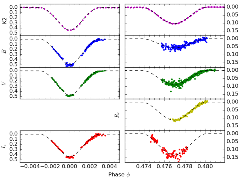
Figure 1: Eclipse photometry compared with binary models. Top row: K2 photometry of the primary and secondary eclipse of WOCS 12009 for the PSF-based approach (Nardiello et al., 2016b). Bottom rows: Ground-based $BVR_{C}I_{C}$ photometry of the primary and secondary eclipses.

After the initial reductions, we found that there were significant color-dependent residuals in the light curves from different stars that resulted from the use of different telescope/camera/filter combinations. These were identified and characterized as linear relations using non-variable stars in the field, but were only judged to be significant in $B$ and $I_{c}$ filters. The correction relations were used to correct all light curves to the system of the MLO filter set as part of the final ensemble photometry analysis. The specific corrections that were applied to WOCS 12009 light curves were less than 0.008 mag for all observational set-ups except one in $I_{c}$ (0.014 mag). The eclipse observations are shown in Fig. 1, and the light curves are provided in tables in the electronic version.

2.3 Spectroscopy

Radial velocities of M67 stars have been monitored over a very long period, and there is a large database of WOCS 12009 observations from different telescope / spectrograph combinations spanning almost 29 years. The earliest 23 observations we use here employed the CfA Digital Speedometers (DS; Latham 1985, 1992), which covered 516.7 to 521 nm around the Mg I b triplet. Additional observations were taken on the 1.5 m Tillinghast reflector at Whipple Observatory using the Tillinghast Reflector Echelle Spectrograph (TRES; Fűrész 2008). TRES spectra contained 51 echelle orders covering the whole optical range and into the near-infrared (from about 386 to 910 nm).

Ten spectroscopic observations were taken as part of the WIYN Open Cluster Survey (WOCS; Mathieu 2000) using the WIYN 3.5 m telescope on Kitt Peak and Hydra multi-object spectrograph instrument (MOS), which is a fiber-fed spectrograph capable of obtaining about 80 spectra simultaneously ($\sim$10 fibers set aside for sky measurements and $\sim$70 for stellar spectra). Observations used the echelle grating with a spectral resolution of 20,000 (velocity resolution $\sim$ 15 km s^-1). The spectra are centered at 513 nm with a 25 nm range that covers an array of narrow absorption lines around the Mg I b triplet. Spectroscopic observations for WOCS 12009 were completed using total integrations of either one or two hours per visit that were split into three sub-integrations to allow for rejection of cosmic rays.

Image processing was done using standard spectroscopic IRAF procedures. First, science images were bias and sky subtracted, then the extracted spectra were flat fielded, throughput corrected, and dispersion corrected. The spectra were calibrated using one 100 s flat field and two bracketing 300 s ThAr emission lamp spectra for separate integration times. A more detailed explanation of the acquisition and reduction of the CfA DS, TRES, and WIYN Hydra observations can be found in Geller et al. (2015).

We also collected two new spectra from the HARPS-N spectrograph (Cosentino et al., 2012) on the 3.6 m Telescopio Nazionale Galileo (TNG). HARPS-N is a fiber-fed echelle that has a spectral resolution $R=115000$ covering wavelengths from 383 to 693 nm. The spectra were processed, extracted, and calibrated using the Data Reduction Software (version 3.7) provided with the instrument.

We obtained archival spectra from two additional sources. Eight archived $H$-band infrared ($1.51-1.70\mu$m) spectra with a spectral resolution $R\sim 22500$ for WOCS 12009 were available from the APOGEE project (Holtzman et al., 2015) on the 2.5 m Sloan Foundation Telescope. Before making our radial velocity measurements, we used APOGEE flags to mask out portions of the spectrum that were strongly affected by sky features, and we continuum normalized the spectra using a median filter. Pasquini et al. (2008) tabulated three radial velocity measurements for the primary star as part of their survey of solar analogs in M67, based on observations from February 2007 using the FLAMES/GIRAFFE spectrograph at the VLT. Their spectra covered 644 to 682 nm, including the H$\alpha$ line, and we obtained the spectra through the ESO Phase 3 Data Archive. We continuum normalized the spectra that had been processed and calibrated through the ESO pipeline.

The radial velocities were derived using a spectral disentangling code following the algorithm described in González & Levato (2006). In each iteration step the spectrum for each component is isolated by aligning the observed spectra using the measured radial velocities for that component and then averaging. This immediately de-emphasizes the lines of the non-aligned stellar component, and after the first determination of the average spectrum for each star, the contribution of the non-aligned star is subtracted before the averaging to improve the spectral separation. The radial velocities can also be remeasured using the spectra with one component subtracted. This procedure is repeated for both components and continued until a convergence criterion is met. We use the broadening function (BF) formalism (Rucinski, 2002) to measure the radial velocities using synthetic spectra from the grid of Coelho et al. (2005) as templates. BFs can significantly improve the accuracy of radial velocity measurements in cases when the lines from the two stars are moderately blended (Rucinski, 2002). In the case of the WOCS 12009 binary, the spectra of the two stars have significant differences, so that lines of each star can usually be identified even when the velocity separation is less than 10 km s^-1. As a result, we can derive reasonably reliable velocities for the two stars at small velocity separations when we couple the disentangling technique (and especially the subtraction of the averaged spectrum of each star) with BFs.

The disentangling procedure requires spectra covering the same wavelength range taken at very different orbital phases, and so we had to work with different subsets of our spectra. The CfA DS spectra covered a wide range of orbital phases, but had a limited wavelength range, and so we disentangled these spectra separately. Many of the spectra had comparatively low signal-to-noise that made it impossible to identify the secondary component. We used all spectra in determining the average spectrum for the primary, but only used the 8 spectra with the most clearly detected secondary component to determine its average spectrum. We were only able to measure reliable velocities for the secondary star from these spectra and two others.

We disentangled the TRES and HARPS-N spectra together because they covered similar wavelength ranges at similar resolution, and because it would have been difficult to disentangle the two HARPS-N spectra on their own. Because the TRES and HARPS-N spectra covered the entire optical range, we decided to disentangle them in the wavelength ranges of individual TRES echelle orders. We selected 14 orders with a large number of strong lines, avoiding the bluest and reddest ends of the optical range (due to low signal on the blue end and telluric lines on the red end). This had the additional benefits that we could determine the stellar velocities as means of the velocities derived from the different orders and also get uncertainty estimates from the standard error of the mean. These uncertainties were typically around 0.08 km s${}^{-1}\;$for the primary star and 0.4 km s${}^{-1}\;$for the secondary.

The WIYN spectra were disentangled on their own because we were able to obtain spectra covering a sufficient set of different phases, although we had to take some care in the selection of spectra used to calculate the averaged spectra for the two stars. We used 8 of the 10 spectra for the brighter primary star, and 6 of the best for the secondary. Uncertainties were initially derived from the BF fits, and were scaled to produce a reduced $\chi^{2}$ values of 1 based on a best Keplerian fit to the WIYN radial velocities alone. Typical uncertainties were around 0.15 km s${}^{-1}\;$for the primary star and 1 km s${}^{-1}\;$for the secondary star.

The APOGEE spectra also had to be disentangled on their own because their spectral range did not overlap with the other datasets. The uncertainty estimate for each APOGEE velocity was generated from the rms of the velocities derived from the three wavelength bands in the APOGEE spectra. This was typically around 0.2 km s${}^{-1}\;$for the primary star and 0.7 km s${}^{-1}\;$for the secondary star. The velocity was corrected to the barycentric system using values calculated by the APOGEE pipeline. We compared our measured velocities for the primary star with those of the APOGEE pipeline, and we found a phase-dependent difference with a sign consistent with the idea that the tabulated APOGEE velocities were pulled slightly ($0.5-1.0$ km s^-1) by the presence of the unmodeled secondary star.

We also ended up disentangling the three FLAMES/GIRAFFE spectra (Pasquini et al., 2008) separately. For two of the three spectra we clearly detected and resolved BF peaks for the secondary star on opposite sides of the primary star peak. For the third spectrum, the BF peaks were moderately blended. However, because the two unblended spectra were at very different orbital phases, we were successfully able to disentangle the spectra in this set and were able to derive velocities for both stars in all three spectra. Reliable uncertainties could not be derived from scatter around a best-fit solution for these measurements on their own, however. As a result, we derived uncertainty estimates from their scatter around the best-fit to the entire velocity dataset.

Finally, we employed one radial velocity measurement from Jones et al. (1999) made in March 1996 using the HIRES spectrograph at the Keck 10m telescope. Because the secondary star was not subtracted from the spectrum before their measurement, it is possible there is a small bias in the direction of the system velocity for that measurement.

Corrections were applied to the velocities from different spectroscopic datasets. For the CfA DS velocities, we used run-by-run corrections derived from observations of velocity standards. Run-by-run offsets measured for the TRES spectra were no more than 17 m s^-1, and although we did apply them, they are much smaller than the measurement uncertainties. Velocity offsets for individual Hydra fibers in the WIYN dataset were determined and applied to the WOCS 12009 spectra, although these were of different sign and no more than about $\pm 0.2$ km s${}^{-1}\;$in general.

Because the synthetic spectra used in disentangling do not account for gravitational redshifts of the stars, our velocities should have an offset relative to velocities derived using an observed solar template. For consistency with the large survey of Geller et al. (2015), we subtracted the combined gravitational redshift of the Sun and gravitational blueshift due to the Earth (0.62 km s^-1) from the velocities we tabulated. We did not apply the gravitational redshift correction to the Jones et al. Keck HIRES velocity because it was derived using a solar template. Based on the derived masses and radii for the stars in the binary, they should have slightly larger gravitational redshifts than the Sun (0.66 and 0.69 km s^-1, versus 0.64 km s${}^{-1}\;$for the Sun) but we did not correct for these small differences. We did, however, allow for different system velocities for the two stars in our fits to allow for effects like this and convective blueshifting that could otherwise affect the measured radial velocity amplitudes $K_{1}$ and $K_{2}$ (and the stellar masses) if not modeled. The measured radial velocities are presented in Table 2.

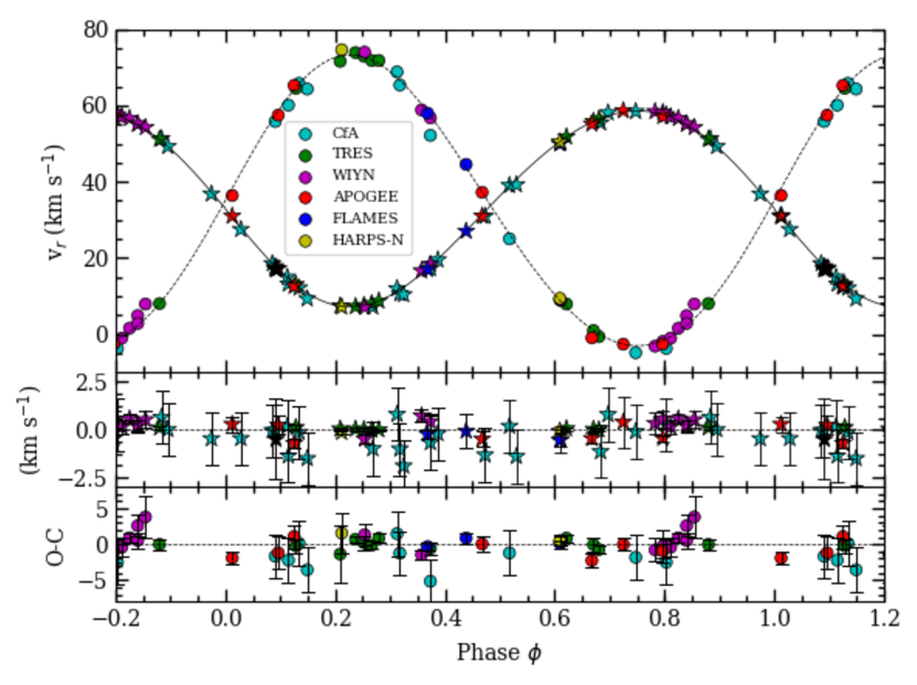
Figure 2: Phased radial velocities for WOCS 12009, along with the best fit model (using the analytic limb darkening law). Measurements for the primary star are shown with star symbols and with circles for the secondary star. The lower panels show the observed minus computed values with error bars scaled to give a reduced $\chi^{2}=1$ (see §3.3).

Even with these corrections to the velocities, we are attentive to the possibility that systematic differences might exist from dataset to dataset. The phased radial velocity measurements are plotted in Fig. 2, showing the best fit to the orbit using all measurements. Among the measured primary star velocities, mean residuals (observed minus computed) were fairly small: 0.18 km s${}^{-1}\;$for WIYN, 0.05 km s${}^{-1}\;$for TRES, $-0.07$ km s${}^{-1}\;$for HARPS-N, $-0.23$ km s${}^{-1}\;$for APOGEE and FLAMES, and $-0.45$ km s${}^{-1}\;$for CfA DS. Because we do not see clear evidence of systematic shifts between spectroscopic datasets, we have not applied any corrections of this sort. We have opted not to scale the uncertainties on the datasets individually, but instead scale uncertainties on all velocity measurements for each star to separately produce a reduced $\chi^{2}$ measurement of 1. This preserves information on the relative precision of measurement in each dataset (which affects their weighting for the final fits) that was most often determined a posteriori. The primary star uncertainties were scaled upward by a factor of 2.1 and the secondary star uncertainties were scaled by a factor of 1.38.

For the purpose of later discussions of the reliability of the stellar mass and radius measurements, we summarize here that we have consistent radial velocity information on both stars from five different spectrographs in a variety of optical and infrared wavelength ranges. This gives us confidence that systematic errors in the radial velocities do not significantly affect the masses and radii we will derive.

3 Analysis

3.1 Cluster Membership

There have been many studies of M67 that have included proper motion measurements and estimations of membership probabilities. All of the studies agree that WOCS 12009 is a highly-probable member. The lowest published membership probability (71%) comes from Zhao et al. (1993), but all others are greater than 93% (Sanders, 1977; Girard et al., 1989; Yadav et al., 2008; Krone-Martins et al., 2010; Nardiello et al., 2016a). In our later use of proper motion membership probabilities to produce a color-magnitude diagram cleaned of field stars, we made use of all of these sources, computing a straight average of all of the probabilities published for each star to assign a final probability.

Geller et al. (2015) also published membership probabilities based on their radial velocity survey, and again WOCS 12009 was assigned high probability of membership (98%). Our modeling of the radial velocities presented below indicates that both stars in the binary have high membership probabilities based on the system velocities we derive: $\gamma_{1}=33.81$ km s${}^{-1}\;$and $\gamma_{2}=33.75$ km s${}^{-1}\;$. Geller et al. found the mean cluster velocity to be 33.64 km s${}^{-1}\;$with a radial velocity dispersion of $0.59^{+0.07}_{-0.06}$ km s^-1.

Based on all of the kinematic evidence, the binary is a high probability cluster member. Additional evidence comes from the distance moduli derived from the radius, $T_{\rm eff}$, and $V$ magnitude of the stars (see §4.2), and from the position of the components of the binary in the CMD once the light from the two stars has been disentangled (see §4.3).

3.2 External Constraints on the Binary

Surface temperature is somewhat important for constraining the limb darkening coefficients to be used in the eclipse modeling (section 3.3), but is even more important for the distance modulus determination in §4.2.

Photometric determinations of $T_{\rm eff}$ using the total system photometry will be affected by the contributions of the secondary star, but the calculation will be a lower limit to the temperature of the primary star and will be closer to the actual temperature the larger the fraction of the system light the primary contributes. Jones et al. (1999) found 5889 K from $BV$ photometry. Using the Stromgren photometry of Balaguer-Núñez et al. (2007) and the $T_{\rm eff}$ calibration of Önehag et al. (2009), we calculate 5920 K from the $(b-y)$ color and a reddening $E(b-y)=0.030$. The APOGEE pipeline provides a temperature of $5950\pm 70$ K from its best fit to its infrared $H$-band spectra using synthetic templates, but again this will be somewhat affected by the light of the secondary star, which is more prominent in the infrared.

With luminosity ratios determined from the binary star analysis below, we are able to separate the light of the two stars and estimate temperatures for them. For this purpose, we used photometry from Sandquist (2004) in the optical along with the color-$T_{\rm eff}$ relations of Casagrande et al. (2010). Assuming a reddening $E(B-V)=0.041\pm 0.004$ (Taylor, 2007), the weighted averages of values computed from ($B-V$) and ($V-I_{C}$) were 6110 K and 4760 K for the primary and secondary stars, respectively. These values are in good agreement with temperatures in the synthetic spectra that optimized our detection of broadening function signal for radial velocity measurement (6000 and 6250 K for the primary, and 4500 and 4750 K for the secondary).

3.3 Binary Star Modeling

To simultaneously model the ground-based radial velocities and photometry and Kepler K2 photometry, we used the ELC code (Orosz & Hauschildt, 2000). We assumed the stars are spherical, and we did not attempt to model spots. The core of the model fit involved a set of 14 parameters: orbital period $P$, time of conjunction (primary eclipse) $t_{c}$, velocity semi-amplitude of the primary star $K_{1}$, mass ratio $q=M_{2}/M_{1}=K_{1}/K_{2}$, systematic radial velocities $\gamma_{1}$ and $\gamma_{2}$, the combinations of eccentricity ($e$) and argument of periastron ($\omega$) $e\cos\omega$ and $e\sin\omega$, inclination $i$, ratio of the primary radius to average orbital separation $R_{1}/a$, ratio of radii $R_{1}/R_{2}$, temperature of the primary $T_{1}$, temperature ratio $T_{2}/T_{1}$, and contamination of the K2 light curve by other sources (independent of the $BVR_{C}I_{C}$ light curves). The K2 contamination parameter is used to account for possible dilution of the light curves by stars that are not physically associated with the binary. Kepler pixels are large by the standards of most ground-based cameras, and in the M67 cluster field, light contamination is a greater concern than in the majority of the field of view. The two stars of greatest significance here are II-216 ($V=19.45$) and WOCS 6008/Sanders 1242 ($V=12.33$), but their distances ($23\arcsec$ and $28\farcs 6$, respectively) will mean that their contributions are relatively small. Because the K2 light curves use long cadence data with 30 minute exposures, they also effectively measure the average flux during a 30 minute exposure. To account for this, the ELC code integrates the computed light curves in each observed exposure window.

Limb darkening is a continuing uncertainty in binary star fits, and to model this we fit for 18 additional parameters using the Kipping (2013) algorithm: two coefficients in the quadratic limb darkening law for each star in the Kepler and $BVI_{C}$ filter bands (and two coefficients for the secondary star in $R_{C}$ because to date we only have secondary eclipse observations). Briefly, Kipping’s algorithm has the advantages that it reduces correlation between limb darkening law parameters, and allows for a straightforward sampling of physically realistic values. We modified the Kipping (2013) algorithm by restricting the second parameter $u_{2}$ to values less than 0.5 in order to force the limb darkening law to be concave down as it approaches the limb. By systematically exploring the parameter space, we can include our limb darkening uncertainties in our uncertainties of the stellar parameters.

The quality of the model fit was quantified by an overall $\chi^{2}$. We applied the temperature of the primary star $T_{1}=6100\pm 100$ K (see §3.2) as an observed constraint, allowing the value to vary but applying a $\chi^{2}$ penalty based on deviation from the determined value. Because the photometric and spectroscopic datasets were pulled together from a variety of sources, the relative weights of different data influences the determination of $\chi^{2}$. For radial velocity measurements, we utilized empirical estimates of measurement uncertainties as much as possible, as described in section 2.3 for each spectroscopic dataset. These empirical measurements were then scaled separately to give a reduced $\chi^{2}$ of 1 for the primary and secondary star datasets. Although some binary star parameters are derived almost exclusively from the velocities, others (like eccentricity $e$ and argument of periastron $\omega$) are affected by the photometry as well, so it is important to try to weight the velocity measurements properly with respect to the photometry. For photometry, we scaled all of the a priori measurement uncertainties upward by the same factor in order to produce a reduced $\chi^{2}$ value of 1 based on separate best fits to data for each filter. Once this was done, we computed simultaneous fits to the photometry and velocity datasets.

The model parameter space was sampled using an implementation of the parallel emcee algorithm (Foreman-Mackey et al., 2013) for Markov chain Monte Carlo. This algorithm allows for efficient sampling of alternate parameter sets using a group of “walkers” (in our case, 1000) that move in parameter space around the values providing the best fit to the data. A proposal for a jump in the position of one walker is taken along a line connecting to, but extending beyond, another randomly chosen walker. The proposed position is accepted with a probability that decreases as $\chi^{2}$ increases. We found that the walkers converged to stable distributions within 2000 steps, and these steps were discarded before forming posterior probability distributions from chains of 6000 step length, skipping every 15 steps. Approximate $1\sigma$ parameter uncertainties were derived from the parts of the posterior distributions containing 68.2% of the remaining models from the Markov chains. The results of the parameter fits are provided in Table 4. In the last column we provide the consensus parameter values for the most important quantities, including a statistical error estimate derived from the results of models in and around the best fit, as well as a systematic error estimate derived from the scatter among the runs with the three different K2 light curves. When there was disagreement, the K2SFF results were generally the outliers. This was particularly noticeable in the luminosity ratios and in the secondary star radius and gravity. We attribute this mostly to the slightly deeper eclipses in the K2SFF light curve, and to a lesser extent to clearly discrepant points during the one observed primary eclipse that had to be deleted. For the radii and gravities, the combined values were derived from an average of the results for all three K2 light curves, while we averaged the results for the PSF-based approach and K2SC light curves for the luminosity ratios. The systematic error quotes reflect these differences.

4 Discussion

For good comparisons of our stellar observations with models, we need to make some assumptions about the chemical composition. The abundances of M67 stars have been studied extensively, and a full review is well beyond what we need here. An important ingredient is abundances measured relative to the Sun, and so here we highlight studies that focused on high-precision differential measurements using Sun-like stars as much as possible. Pace et al. (2008) studied 6 solar analogs in M67 (and a solar spectrum) to derive [Fe/H]$=+0.03\pm 0.04$ (standard deviation), and Santos et al. (2009) gets $+0.01\pm 0.04$ from the same 6 dwarf spectra. Önehag et al. (2011) did a strictly differential comparison of the solar twin Sanders 770, and obtained [Fe/H]$=+0.023\pm 0.015$. Liu et al. (2016) conducted a strictly differential comparison of two solar twins in M67 (including a high resolution solar spectrum reflected from the asteroid Hebe that was taken with the same set-up), finding [Fe/H]=$-0.005\pm 0.010$ for Sanders 770 and $-0.061\pm 0.014$ for Sanders 1462. Those authors interpreted the difference in [Fe/H] between the two stars as significant.

Önehag et al. (2014) did a differential comparison of 14 M67 stars on the main sequence, turnoff, and subgiant branch relative to the solar twin Sanders 770. Those authors find that M67 stars have abundance patterns very similar to that of the Sun, and perhaps even more so than solar twin candidates in the solar neighborhood. Their averaged abundances for all their measured heavy elements except Li was [X/H]$=-0.017\pm 0.003$. They also found that the main sequence and turnoff stars in their sample were slightly depleted in heavy elements compared to subgiants, possibly due to the action of diffusion.

In a differential sense, M67 photospheric metallicities agree with the Sun’s within about $\pm 0.03$ dex, although diffusion may affect the abundances for a subset of M67 stars at similar level. It should be remembered, however, that the bulk metal content of the Sun is still uncertain (e.g. Asplund et al., 2009; Caffau et al., 2011), and will remain an obstacle to a comprehensive analysis of M67 stars.

4.1 Mass and Radius

The masses and radii of the eclipsing stars are important because they are high-precision, distance- and reddening-independent, measurable characteristics. In the case of M67, these kinds of measurements can potentially provide strong constraints on the cluster age.

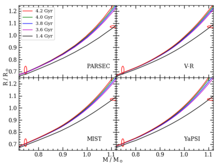
Figure 3: Mass-radius plot for the members of S1247 with $2\sigma$ uncertainties indicated by the error ellipses. Models use $Z=0.0152$, 0.0188, 0.0142, and 0.0162, respectively for PARSEC (Bressan et al., 2012), Victoria-Regina (VandenBerg et al., 2006), MIST (Dotter, 2016; Choi et al., 2016), and YaPSI (Spada et al., 2017) isochrones.

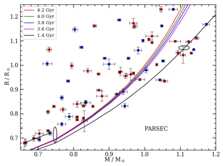
Figure 4: Mass-radius plot for the members of S1247, along with precisely measured stars from eclipsing binaries (Southworth, 2015). Isochrones have the same meaning as in Fig. 3. Primary stars in the eclipsing binaries are blue, and secondary stars are red. All error bars and ellipses use $2\sigma$ uncertainties. Black lines connect the members of binaries V404 CMa (Rozyczka et al., 2009) and ASAS J082552-1622.8 (Hełminiak & Konacki, 2011), having stars with masses similar to that of WOCS 12009 B.

In Fig. 3 we compare the results of our binary star model fits with theoretical expectations from isochrones, and in Fig. 4 we compare against precisely measured members of eclipsing binaries (Southworth, 2015). For the comparisons in the figures, the error ellipses for WOCS 12009 include contributions from statistical and systematic error added in quadrature, and we have employed the chemical compositions used by the modellers in calibrating their isochrones to the Sun. The properties of the secondary star (WOCS 12009 B) are in rough agreement with isochrone predictions, although there is some dependence on the chemical composition and the implementation of the stellar physics in the models. Also of note, the secondary star is slightly closer to the isochrones than any other star in the range from about $0.7-0.8M_{\odot}$. This is probably because WOCS 12009 B is in a much longer period binary than other measured main sequence stars. For example, V404 CMa (Rozyczka et al., 2009) has a period of just 0.452 d, and ASAS J082552-1622.8 (Hełminiak & Konacki, 2011) has a period of 1.528 d. Tidal interactions and the resulting stellar activity are likely to be responsible for the relatively large radii in systems like those (see Torres et al. 2010 and references therein). WOCS 12009 B is probably a better approximation to a star that has evolved in isolation, and is therefore valuable in its own right.

On the other hand, while the primary star (WOCS 12009 A) has characteristics putting it among other well-measured eclipsing stars in the field, it is much smaller than predicted for its mass and reasonable ages for M67. Isochrone fits to the CMD have returned ages from about 3.5 Gyr to 4.0 Gyr (Sarajedini et al., 2009) and 3.6 to 4.6 Gyr (VandenBerg & Stetson, 2004), with a large part of these ranges resulting from model physics and chemical composition uncertainties. Stello et al. (2016) quote an age of about 3.5 Gyr from their asteroseismic analysis of pulsating giants in M67. The disagreement between WOCS 12009 A’s radius and the predictions from models with ages at the low end of the range quoted for M67 is more than 15%. The star’s radius is larger than that of a zero-age main sequence star, and is consistent with a star of approximately 1.4 Gyr age.

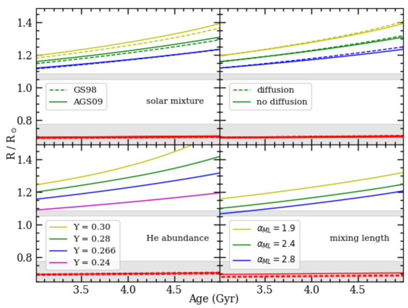
Figure 5: Radius evolution of stars of $0.75M_{\odot}$ (red lines) and $1.12M_{\odot}$ stars when model composition and physics inputs are varied. Grey rectangles show the $2\sigma$ uncertainty range for the measured radii of WOCS 12009 stars. In the top two panels, tracks for [Fe/H] $=-0.1$ (yellow lines), 0.0 (green lines), and $+0.1$ (blue lines) are shown.

To illustrate the difficulties in explaining the mass and radius of this star consistently with the cluster age, we explored one-dimensional stellar evolution models (Fig. 5). Stellar models were calculated using the 1-D Yale Rotating Evolution Code (YREC; Pinsonneault et al. 1989), using the nuclear cross-sections, opacities, equations of state, and model atmospheres described in section 2.3 of Somers & Pinsonneault (2016). For the base model, we adopt the Asplund et al. (2009) present-day solar photospheric abundance ratio $Z/X=0.0181$, assume helium and heavy metal diffusion as calculated by Thoul et al. (1994), calibrate the solar mixing length and helium abundance to reproduce the solar luminosity and radius at 4.57 Gyr, and assume no rotation. As parameter variations, we test the alternate solar mixture given by Grevesse & Sauval (1998), assume diffusion-less envelopes, adopt different proto-solar helium abundances, vary the convective efficiency by changing the mixing length (e.g. Chabrier et al. 2007), and permit modest core overshooting of $\sim 0.2$ pressure scale heights.

The secondary star’s characteristics are less sensitive to uncertainties in age, stellar physics, and composition than the primary star’s are, so that the overall agreement of models and observations of the secondary is a useful validation. Reasonable changes to the chemical composition of the stars are unable to explain a radius discrepancy of this magnitude, although higher metallicity or lower helium abundance would push the models in the right direction. In the case of helium alone, the abundance would have to be moved in a direction opposite what is observed for galactic chemical evolution and reduced below Big Bang nucleosynthesis values ($Y=0.245$) to come close to the observed radius. The metallicity of M67 stars has been repeatedly shown to be very close to solar, and so to explain the radius discrepancy with metallicity would require a change several times any reasonable uncertainty in M67’s value.

Stellar physics uncertainties also seem to fall short of explaining the small radius. The inclusion of diffusion makes a model star marginally larger, and so this cannot alleviate the issue. More efficient convection (through a larger mixing length parameter $\alpha_{ML}$, for example) can produce a smaller star, but again, an explanation of the radius issue would require a large change. For a star with a thinner surface convection zone than the Sun, convection is expected to be less efficient due to radiative losses. Convective core overshoot tends to make the star slightly smaller, but even for overshoot several times larger than inferred from cluster comparisons (0.2 pressure scale heights), this effect is also too small by a factor of at least three.

To summarize, we find no chemical composition or stellar physics uncertainties that can explain the small size of the star WOCS 12009 A.

4.2 Distance Modulus

We can further test the membership of the binary by deriving the luminosity of each star, and by comparing the absolute with the apparent magnitudes. The photometry of the two stars was deconvolved using luminosity ratios from the multi-filter light curve analysis, and photometric temperatures were derived from the colors and cluster reddening (see section 3.2). The temperatures, along with radii derived from the binary analysis and theoretical bolometric corrections from Casagrande & VandenBerg (2014), allow us to derive the absolute magnitudes $M_{V}$. We find $(m-M)_{V}=9.74\pm 0.03$ and $9.82\pm 0.09$ for the primary and secondary stars respectively. The quoted uncertainties include contributions from the measurement of the apparent magnitudes, the calculation of the luminosity, and the calculation of the bolometric correction. These values are in excellent agreement with each other and with previous measurements of M67’s distance modulus. For comparison, some notable recent measurements are $9.76\pm 0.06\pm 0.05$ (statistical and systematic uncertainties) from 10 solar analogs (Pasquini et al., 2008), $9.72\pm 0.05$ using metal-rich field dwarfs with Hipparcos parallaxes (Sandquist, 2004), and $9.70\pm 0.04$ from K2 asteroseismology of more than 30 cluster red giants (Stello et al., 2016).

4.3 The Color-Magnitude Diagram (CMD)

With well-studied binary stars, we can bring important and rarely available new mass information to the study of the color-magnitude diagram and to the comparison of observational data with theoretical models. To that end, we used luminosity ratios derived from the binary star modeling to deconvolve the light in different wavelength bands for the two WOCS 12009 stars, and determine their CMD positions. In the discussions below, we use the high-precision photometry of Sandquist (2004) along with the identifications for high-probability single-star members from that study. The original list was selected based on being at the blue edge of the band of main sequence and binary stars in the CMD, but we have verified that the majority of the list were classified as single members with no detectable radial velocity variability by Geller et al. (2015). Those that were identified as binaries were eliminated. So to the greatest degree we can, these stars should trace out where the main sequence and turnoff should be for the age of M67.

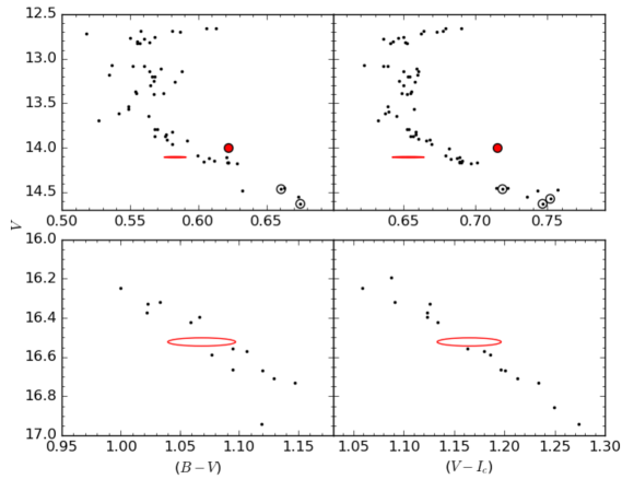
Figure 6: Color-magnitude diagrams of M67 zoomed near the components of WOCS 12009. Small points are probable single-star members with photometry from Sandquist (2004) and circles are solar analogs identified by Pasquini et al. (2008). The system photometry for WOCS 12009 is shown with a red circle, and $2\sigma$ error ellipses for the deconvolved photometry of the component stars are shown in red.

Because the statistical uncertainties in the system photometry are well below 0.01 mag and the system photometry has been calibrated in the same way as the rest of the cluster stars we use in the CMDs, the relative photometry should be reliable. In the CMDs (see Fig. 6), the secondary star falls among probable single main sequence stars at $V\approx 16.5$. The primary star is slightly bluer than the main sequence at $V\approx 14.1$, as we would expect for a star that is less evolved than the other cluster stars.

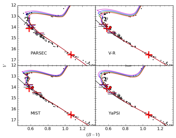
Figure 7: ($B-V$,$V$) color-magnitude diagram for the turnoff and main sequence of M67. Small points are probable single-star members from Sandquist (2004) and circles are solar analogs identified by Pasquini et al. (2008). The system photometry for WOCS 12009 is shown with a red circle, and deconvolved photometry of the component stars are red crosses. Isochrones are from the PARSEC ($Z=0.0152$), Victoria-Regina ($Z=0.0188$), MIST ($Z=0.0142$), and Yale-Potsdam ($Z=0.01619$) sets for ages of 1.4, 3.6, 3.8, 4.0, and 4.2 Gyr, and have been shifted to match the mass and photometry of the secondary star of WOCS 12009. The theoretical predictions for stars with masses equal to the primary star of WOCS 12009 ($V\approx 13.8-14.0$) and to the Sun ($V\approx 14.6-14.7$) are shown with horizontal lines.

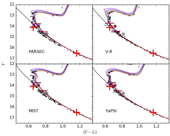
Figure 8: Same as for Fig. 7 except for ($V-I_{C}$,$V$) photometry.

When we shift isochrones to force a fit to the mass and photometry of the secondary star (see Figures 7 and 8), there is decent agreement between the cluster main sequence stars and the theoretical predictions for the V-R and MIST isochrone sets. The landscape is similar for the ($V-I_{C}$,$V$) CMD (see Fig. 8), although the MIST isochrones don’t match the main sequence as well.

The mass of the primary star would be a more valuable constraint on the masses of evolved stars in the cluster and on the cluster’s age if it had had a conventional evolution history. However, if we utilize the model isochrones in a relative sense, we can infer with some confidence that a single cluster star with the mass of WOCS 12009 A (about $1.11M_{\odot}$) and an uneventful evolution history should reside at $V\approx 13.8$, about 0.35 mag brighter than WOCS 12009 A and just faintward of the “hook” feature in the CMD. Models tied to WOCS 12009 B also predict that a solar mass star in M67 should have $V\approx 14.57$. This is quite close to the $V$ magnitude of the star Sanders 1095 (1787 in Yadav et al. 2008) that Pasquini et al. (2008) identified as one of their two best solar analogs.

In the CMD, the turnoff of M67 potentially gives us a lot of insight into the physics of the stellar cores. Our group is currently working on additional binary systems that will allow us to identify the precise masses of stars at the turnoff, and so we will not undertake a full discussion of the topic here. The CMDs in Figures 7 and 8 illustrate the substantial differences in the isochrones produced by different groups, and without clarity on the “correct” physics and chemical composition inputs to include in the models, systematic errors in the cluster age will be unavoidable.

The noticeable gap seen at $V\approx 12.9$ is an indicator of rapid evolution through that part of the CMD, probably due to the presence of a small convective core maintained by CNO cycle hydrogen burning reactions and their strong temperature dependence. However, there are several composition and physics factors that can affect the size (and even the presence) of a convective core in models. VandenBerg et al. (2007) and Magic et al. (2010) studied extensive sets of stellar models to try to identify the important factors, but Magic et al. in particular found that there are degeneracies in how the CMD is affected. Composition factors like the metallicity of M67 relative to the Sun and the actual solar mixture affect the abundance of CNO cycle catalyst nuclei, while physics like diffusion, the prescription for convective core overshoot, and CNO cycle reaction rates can affect the strength of the energy release in the stellar cores. While some of the models approximately reproduce the brightness of the gap (which occurs in the straight-line segment immediately faintward of the bluest point on the isochrone), models generally are not as successful in matching the blue protrusion among the M67 main sequence stars at $V\approx 13.7$. To the extent that we are able to check with current models, the cluster CMDs are consistent with typically quoted ages of $3.8-4.2$ Gyr.

4.4 Stellar Motions and Li Abundance

Every indication we have is that the binary WOCS 12009 is a member of the M67 cluster, but the primary star is significantly smaller than expected for reasonable cluster ages, and it is also hotter and less luminous than expected for its mass. Before discussing possible explanations, we assemble other observations that can comment on the puzzle.

Using our highest resolution spectroscopic observations (with the TRES and HARPS-N spectrographs), we looked at the rotational motions of the two stars in the binary, but were unable to detect rotation in the broadening functions of the two stars. The upper limits are $v_{\rm rot}\sin i<5$ km s${}^{-1}\;$from the TRES observations and $<4$ km s${}^{-1}\;$from the HARPS-N observations. Although slow rotation is expected for single solar-type stars in an old cluster like M67, the low rotation speed of the primary has some impact on our understanding of its genesis, as discussed later.

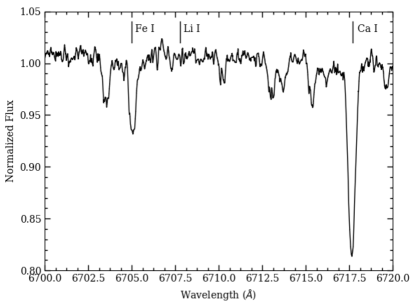
Figure 9: The averaged FLAMES spectrum for WOCS 12009 A in the vicinity of the Li I resonance doublet.

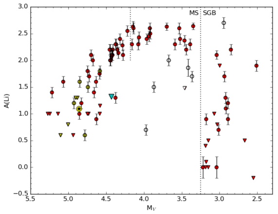
Figure 10: Li abundances ($A(\mbox{Li})=\log(N_{\mbox{Li}}/N_{\mbox{H}})+12$; Pace et al. 2012) as a function of absolute magnitude $M_{V}$, assuming a distance modulus $(m-M)_{V}=9.72$. Red symbols indicate probable single stars, yellow symbols are the Sun ($\odot$) and solar twin candidates (Pasquini et al., 2008), red triangles are upper limits, and white symbols are stars identified as deviant by Pace et al.. The blue arrowhead is the upper limit for WOCS 12009 A (Jones et al., 1999). The dotted line at $M_{V}=4.19$ shows the expected position of normal cluster star with WOCS 12009 A’s mass.

The mass of WOCS 12009 A should place it at the faint end of the cluster’s Li plateau with abundances $A(\mbox{Li})\approx 2.5$ (Pace et al., 2012). Stars in the plateau have outer convective zones that do not mix Li atoms down to temperatures where nuclear reactions can burn them, and additional mixing processes must have little if any effect. Even with the diluting effects of the secondary star’s light on the Li lines, Li should have been detectable if it was present with the plateau abundance. Our spectral disentangling allows us to mostly remove the secondary star’s contribution to the spectrum and to produce an average spectrum for the primary star as a byproduct. The averaged FLAMES spectrum for the primary is shown in Fig. 9, as it has the highest signal-to-noise in that wavelength range. There is still no sign of the Li lines for the primary star. Jones et al. (1999) provide an upper limit for the system ($A(\mbox{Li})<1.32$) that puts the star’s abundance at least about 0.8 dex lower than stars at the same absolute magnitude, but because the star is probably underluminous compared to normal cluster stars of the same mass (see §4.3), the discrepancy is more than an order of magnitude (Fig. 10).

4.5 The Formation of the Primary Star

The Li observations could be explained by a stellar union: stars of about $0.95M_{\odot}$ or less would have depleted their surface Li to undetectability well before the present age of the cluster because the surface convection zone easily reaches down to Li burning temperatures. In the union of two such stars, a more massive star with depleted Li would result.

This could also explain the smaller than expected radius of the primary star. In hydrodynamic simulations of stellar collisions, it is found that the material from the two stars gets sorted radially in the merger remnant by entropy to good approximation (Lombardi et al., 2002). Because lower mass stars have lower temperatures and higher densities in their cores, the core of the lower mass star ends up at the core of the remnant. This effectively restarts the remnant with a higher core hydrogen content, and makes it look like a younger main sequence star once a Kelvin-Helmholtz timescale has passed and the remnant has thermally adjusted to its new structure. As a result, if the star’s size makes it look like it is 1.4 Gyr old now, that is likely to be fairly close to the time elapsed since a merger took place.

Two stars could combine as part of the merger of a close binary pair or the collision of two stars during a resonant multi-star interaction. Both are likely to produce a remnant that is depleted of surface Li, but the route for combining the stars could leave signatures on their motions. Is there a reasonably probable mechanism that could produce a slowly rotating remnant star in wide low eccentricity ($e=0.05$) binary?

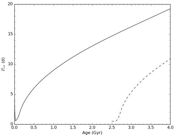
Figure 11: Rotational evolution for $1.1M_{\odot}$ stellar models having a single-star evolutionary history (solid line) and having a birth as a stellar merger 1.5 Gyr before the present day (dashed line).

Unless the combining stars were in a nearly head-on collision, the remnant star is likely to have started with rapid rotation. The primary star in WOCS 12009 probably has a surface convection zone though, meaning that some spindown via a magnetic wind is likely. If the remnant was made approximately 1 Gyr ago, we can ask whether there was sufficient time for it to spin down as an effectively single star. The rotation of stars in the 1 Gyr old cluster NGC 6811 was studied during the Kepler mission (Meibom et al., 2011). In that cluster, stars with $(B-V)$ color similar to WOCS 12009 A have spun down from their zero-age main sequence values to a period of around 10 d. For a star the size of WOCS 12009 A, a 10 d period roughly corresponds to rotation near our $v_{\rm rot}\sin i$ detection limit of 5 km s^-1. We computed rotational stellar models using YREC (see section 4.1) to check this idea further, as shown in Fig. 11. A $1.1M_{\odot}$ star has enough of a surface convection zone that spindown via a magnetic wind could bring a rapidly rotating star (modeled here with a period $P_{\rm rot}=0.5$ d) down to our detection limit in 1.5 Gyr. A detected rotation period for the primary, as opposed to our current upper limit, could in principle be used to infer the time since merger, for the same reason that a rotation period for a single non-interacting star can be used as an age indicator. This would be one interesting test of the merger hypothesis.

It is plausible that a rapidly rotating merger remnant could have spun down to the levels we see today, but other observations may test this. For example, the Ca II H and K emission index (an activity indicator) has been measured for WOCS 12009 by Giampapa et al. (2006), and they find that it has a relatively high value relative to other M67 stars, but not out of the range of the best vetted single star candidates (Curtis, 2017). Mamajek & Hillenbrand (2008) compute $\log R\arcmin_{\rm HK}=-4.70$ from the Giampapa et al. data, which probably makes it more active than the 95% range for the Sun. An examination of spot modulation on the primary star might also be able to reveal whether it is rotating significantly more rapidly than single cluster stars of similar color. Such measurements are currently underway under the umbrella of the K2 M67 Study.

The other major question is whether the orbital characteristics of the current binary could be natural products of any potential formation mechanisms. Below we consider stellar collisions and the evolution of hierarchical triple systems.

A stellar collision during a multi-body dynamical interaction is a relatively common outcome if the incoming binary (or binaries) are tightly bound. Fregeau et al. (2004) examined binary-single and binary-binary scattering experiments with collisions allowed, and found as expected that low eccentricities are strongly disfavored in binaries formed after stellar collisions — the conditions required for the outgoing stars to wind up on a nearly circular orbit are too narrow. Even with a maximal amount of expansion by a merger remnant before it thermally relaxes, tidal interactions are unlikely to be able to help circularize the orbit of WOCS 12009, which is currently relatively wide ($a/R_{1}\approx 82$).

Formation involving a hierarchical triple system that dynamically formed as part of a multi-body interaction along with the subsequent merger of the close pair faces some of the same difficulties. For guidance, we examined the scattering study of Antognini & Thompson (2016). Those authors find that when triple systems are dynamically formed, a compact configuration (with the ratio of the outer orbit periastron to the inner orbit semi-major axis $r_{\rm P,outer}/a_{\rm inner}\sim 10$) is a preferred outcome. If the current orbit of WOCS 12009 corresponds to the outer orbit of such a compact triple, the inner orbit could have had a period of around 2 d. This is long enough that the inner binary would not have merged rapidly via tidal interactions or magnetic braking. However, an eccentricity as low as 0.05 for the outer orbit is again strongly disfavored as part of the dynamical formation of the triple.

A primordial triple system with an inner binary that merges after about 3 Gyr is also a possibility. First considering the low eccentricity of the current orbit, we note that low eccentricity binaries with periods above $10^{4}$ d are known among solar-type binaries in the field (Raghavan et al., 2010). A few percent of binaries with orbital solutions in the 2.5 Gyr old cluster NGC 6819 (Milliman et al., 2014), in M67 (Pollack et al., 2017), and the 7 Gyr old cluster NGC 188 (Geller et al., 2009) are known to have $e<0.1$ and $P>20$ d. (For NGC 6819 and M67, there are known long-period systems with $e<0.06$.) For known triple systems, the outer orbit is usually eccentric, but there are known examples with $e<0.05$. So it is not out of the question to think that the low eccentricity can result from the star formation process.

The inner binary might have formed with an initial period near 2 d as part of the star formation process, allowing angular momentum loss mechanisms like tides and magnetic braking (Stȩpień, 2011, e.g.,) to produce a merger. The majority of the time ($\sim 2-3$ Gyr) would be needed to have the binary lose enough energy to come into contact and ultimately merge. M67 systems AH Cnc, EV Cnc, and HS Cnc are contact or near-contact binaries near the cluster turnoff (Stassun et al., 2002; Sandquist & Shetrone, 2003; Pribulla et al., 2008; Yakut et al., 2009) that could be in this stage of their orbital evolution, and theoretical studies indicate that sub-turnoff mergers could be of order 3-4% of the upper main sequence population for an old cluster like M67 (Andronov et al., 2006).

A primordial triple with an inner binary having a period substantially longer than 3 days might also be capable of producing a system like WOCS 12009, but stability against disruption is a concern if the inner binary has too long a period. As a guide, Mardling & Aarseth (2001) used a criterion for stability against escape of a component star that implies $r_{\rm P,outer}/a_{\rm inner}\sim 3.4$ for the WOCS 12009 system, which translates to an inner orbit with $a_{\rm inner}\approx 0.12$ AU or $P_{\rm inner}\approx 14$ d. For an inner binary formed with an initial period closer to 14 d, Kozai-Lidov oscillations due to the third star would probably be needed to drive the binary’s eccentricity up before tidal dissipation could produce a shorter period (Fabrycky & Tremaine, 2007). This would require misalignment of the inner and outer orbital planes, but Kozai-Lidov cycles can have a very short timescale (comparable to but longer than the period of the outer orbit), so that there would be no difficulty with producing a close binary within the age of M67. Once close binary interactions become dominant, Kozai cycles are suppressed and the binary is expected to evolve as if it is isolated from the third star.

For a stable primordial triple formed with an outer orbital period near 70 d, either of these paths would likely result in a circularized inner binary with a period of a few days, which will later merge. If a Kozai mechanism was responsible for the initial stage of decreasing the separation of an inner binary system, we might be able to observe the signature of an inclination difference between the orbit of the inner binary and the orbit of the teriary star (Fabrycky & Tremaine, 2007). The rotation axis of the merged star would probably retain the direction of the angular momentum vector for the close binary. Because the current system reflects the orbital plane of the outer binary in the original triple and because the binary is currently eclipsing, the rotation axis of the primary star could be inclined to our line of sight by about $40\arcdeg$. Thus, depending on its axial orientation, it might be possible to observe muted rotational effects such as the Rossiter-McLaughlin effect on the radial velocities or rotational modulation of the light curve.

5 Conclusions

We present high-precision measurements of the masses, radii, and photometry for stars in the bright detached eclipsing binary system WOCS 12009 in the cluster M67. This cluster is commonly used as a testbed for stellar evolution models of solar metallicity, and the addition of new observables for stars in the cluster will further test the fidelity of the physics we use to model them. We are currently in the process of analyzing other eclipsing cluster binaries that will expand these tests to higher and lower mass stars in M67.

For the WOCS 12009 system, we find that the primary star is substantially smaller than expected from any reasonable evolution model for a single star of its mass. This, as well as the non-detection of photospheric Li, and its relatively high temperature and low luminosity, points us toward an explanation involving a merger of two lower mass stars. The low rotation rate of the primary star appears to be explicable if a merger took place more than about a billion years ago, as this would give the remnant star time to spin down as an effectively single star. The long-period, low eccentricity orbit of the binary is harder to understand, as most dynamical interactions in the cluster should have resulted in eccentricity that could not have been eliminated in the age of the cluster. Our preferred explanation is that this was born as a compact hierarchical triple system, and tidal interactions (possibly assisted by Kozai-Lidov oscillations) eventually brought the system into contact and led to a merger.

Regardless of the mechanism behind its formation, the primary star might have been identified as a blue straggler had it not had a cool companion that reddened the binary’s combined light. Even so, the primary star has a low enough mass that it is only slightly bluer than the cluster main sequence. However, as the cluster ages and single stars of the same mass evolve off the main sequence, this star will retain its youthful main sequence appearance for an extra $2-3$ billion years and will be more clearly identifiable as a product of unusual circumstances.

Table 1: Ground-Based Photometric Eclipse Observations

UT Date	Filters	mJD Start	$N_{obs}$	Telescopes
2003 Apr. 21	$I_{c}$	2750.63952	150	MLO
2004 Jan. 26	$V$	3029.63023	168	LaS
2016 Jan. 1	$BVI_{c}$	7389.40312	58,61,62	CPT
2016 Feb. 3	$BVR_{c}$	7422.55368	98,146,96	ELP,LSC,MLO
2016 Apr. 13	$BVI_{c}$	7492.22555	72,69,77	CPT
2016 May 20	$BVI_{c}$	7528.65024	30,31,33	MLO,OGG

Table 2: Radial Velocity Measurements

mJD	$v_{A}$	$\sigma_{A}$	$v_{B}$	$\sigma_{B}$	mJD	$v_{A}$	$\sigma_{A}$	$v_{B}$	$\sigma_{B}$
	(km s-1)		(km s-1)			(km s-1)		(km s-1)
CfA Observations					WIYN Observations
47200.90558	51.31	0.66			54100.95996	55.15	0.16	4.93	1.13
47216.87938	15.03	0.66			57407.00468	7.16	0.12	73.96	1.04
47230.82288	12.04	0.66	68.78	2.26	57443.91188	58.43	0.26	-3.08	1.19
47489.89727	27.54	0.66			57444.90238	58.17	0.21	-1.83	1.62
47493.89927	18.58	0.66			57445.88308	57.07	0.19	-0.97	1.00
47495.93427	13.24	0.66	60.08	2.26	57446.87188	56.63	0.12	1.63	0.46
47513.97706	17.29	0.66	52.15	2.26	57447.91718	55.21	0.13	2.90	0.80
47524.02176	39.05	0.66	25.05	2.26	57448.89118	54.27	0.21	7.97	2.13
47543.94386	57.58	0.66	-3.66	2.26	57762.88603	16.68	0.16	58.84	0.41
47555.88246	36.83	0.66			57764.00282	18.38	0.18	56.75	0.63
47579.82666	10.70	0.66	65.36	2.26	HARPS-N Observations
47609.78406	58.44	0.66	-4.78	2.26	57752.73729	7.25	0.055	74.59	2.01
47633.71796	17.82	0.66	55.80	2.26	57780.44623	50.45	0.027	9.46	0.56
47636.74956	12.20	0.66	65.80	2.26	APOGEE Observations
47846.96906	9.36	0.66	64.30	2.26	56654.92723	31.01	0.19	37.24	0.83
47898.98907	49.28	0.66			56668.86973	55.17	0.14	-0.90	0.73
47928.94617	10.47	0.66			56698.75512	17.31	0.24	57.44	1.65
47994.75116	7.23	0.66			56672.86367	58.64	0.64	-2.56	0.64
48023.69056	55.46	0.66			56677.88291	57.16	0.07	-2.51	0.68
48024.64486	58.09	0.66			56700.76763	12.64	0.12	65.24	1.14
48281.93347	19.56	0.66			56734.66629	50.21	0.33	8.88	0.6
48291.90987	39.26	0.66			56762.63516	31.02	0.20	36.42	0.6
54424.00437	30.99	0.66			FLAMES Observations
TRES Observations					54137.78614	17.07	0.13	57.97	0.35
57362.92518	51.81	0.037	7.97	0.41	54142.68654	27.07	0.44	44.55	0.52
57403.90238	7.48	0.040	71.57	2.88	54154.58411	49.96	0.17	9.13	0.23
57405.85138	7.34	0.043	73.85	0.36	Keck HIRES Measurement
57406.92938	7.63	0.047	72.88	0.67	50143.94133	17.4
57407.90858	8.11	0.047	71.78	0.38
57408.81588	8.80	0.026	71.77	0.46
57436.77248	56.43	0.035	-0.57	0.43
57450.68408	51.18	0.047	8.10	0.55
57714.99979	55.83	0.038	1.00	0.64
57746.91989	13.08	0.056	64.48	0.72

Table 3: Out-of-Eclipse Photometry for WOCS 12009

Filter	S04	YBP	MMJ	Filter	2MASS
$B$	$14.6161\pm 0.0038$	$14.646\pm 0.008$	$14.663$	$J$	$12.785\pm 0.021$
$V$	$13.9942\pm 0.0005$	$14.007\pm 0.003$	$14.044\pm 0.05$	$H$	$12.459\pm 0.023$
$I_{C}$	$13.2792\pm 0.0007$	$13.283\pm 0.001$	$13.266$	$K_{S}$	$12.422\pm 0.023$

Note. — S04: Sandquist (2004). YBP: (Yadav et al., 2008). MMJ: Montgomery et al. (1993). 2MASS: Skrutskie et al. (2006).

Table 4: Best-Fit Model Parameters for WOCS 12009

Parameter	K2 Light Curves/Limb Darkening Law			Combined
	PSF-based Approach LC	K2SC LC	K2SFF LC
$T_{1}$ (K)	$6100\pm 100$ (constraint)
$\gamma_{1}$ (km s${}^{-1}\;$)	$33.815\pm 0.009$	$33.814\pm 0.009$	$33.815\pm 0.009$	$33.815\pm 0.009$
$\gamma_{2}$ (km s${}^{-1}\;$)	$33.745\pm 0.010$	$33.746\pm 0.009$	$33.745\pm 0.010$	$33.745\pm 0.009$
$P$ (d)	69.728087	69.728107	69.728117
$\sigma_{P}$ (d)	0.000014	0.000013	0.000014
$t_{C}-2450000$	7180.14126	7180.14068	7180.14063
$\sigma_{t_{C}}$	0.00012	0.00012	0.00016
$i$ ($\arcdeg$)	$89.565\pm 0.019$	$89.568\pm 0.016$	$89.637\pm 0.013$
$q$	$0.674\pm 0.004$	$0.674\pm 0.004$	$0.674\pm 0.003$	$0.674\pm 0.004$
$e\cos\omega$	$-0.036166\pm 0.000009$	$-0.036126\pm 0.000010$	$-0.036134\pm 0.000005$
$e\sin\omega$	$0.0377\pm 0.0016$	$0.0376\pm 0.0016$	$0.0361\pm 0.0016$
$e$	$0.0522\pm 0.0012$	$0.0522\pm 0.0011$	$0.0510\pm 0.0011$
$\omega$ ($\arcdeg$)	$133.7\pm 1.1$	$133.8\pm 1.2$	$135.1\pm 1.3$
$K_{1}$ (km s-1)	$25.64\pm 0.04$	$25.65\pm 0.04$	$25.63\pm 0.04$	$25.64\pm 0.04$
$K_{2}$ (km s-1)	$38.06\pm 0.19$	$38.06\pm 0.20$	$38.05\pm 0.22$	$38.06\pm 0.20$
$R_{1}/R_{2}$	$1.447\pm 0.042$	$1.460\pm 0.035$	$1.537\pm 0.020$
$R_{1}/a$	$0.01221\pm 0.00007$	$0.01221\pm 0.00008$	$0.01225\pm 0.000014$
$R_{2}/a$	$0.00844\pm 0.00025$	$0.00836\pm 0.00021$	$0.00797\pm 0.00016$
$T_{2}/T_{1}$	$0.770\pm 0.005$	$0.772\pm 0.006$	$0.772\pm 0.006$
K2 contam.	$0.031\pm 0.004$	$0.0027\pm 0.0029$	$0^{+0.0003}$
$L_{2}/L_{1}(B)$	$0.0694\pm 0.0049$	$0.0686\pm 0.0043$	$0.0655\pm 0.0028$	$0.0690\pm 0.0049\pm 0.0004$(sys)
$L_{2}/L_{1}(V)$	$0.1081\pm 0.0067$	$0.1076\pm 0.0055$	$0.0940\pm 0.0025$	$0.1079\pm 0.0067\pm 0.0003$(sys)
$L_{2}/L_{1}(R)$	$0.1439\pm 0.0090$	$0.1420\pm 0.0070$	$0.1209\pm 0.0033$	$0.1429\pm 0.0090\pm 0.0010$(sys)
$L_{2}/L_{1}(I)$	$0.1724\pm 0.0099$	$0.1734\pm 0.0096$	$0.1554\pm 0.0052$	$0.1729\pm 0.0099\pm 0.0005$(sys)
$M_{1}/M_{\odot}$	$1.109\pm 0.015$	$1.112\pm 0.013$	$1.111\pm 0.014$	$1.111\pm 0.015$
$M_{2}/M_{\odot}$	$0.749\pm 0.005$	$0.749\pm 0.005$	$0.747\pm 0.006$	$0.748\pm 0.005$
$R_{1}/R_{\odot}$	$1.070\pm 0.008$	$1.070\pm 0.007$	$1.073\pm 0.006$	$1.071\pm 0.008\pm 0.003$(sys)
$R_{2}/R_{\odot}$	$0.739\pm 0.019$	$0.732\pm 0.016$	$0.699\pm 0.010$	$0.713\pm 0.019\pm 0.026$(sys)
$\log g_{1}$ (cgs)	$4.425\pm 0.006$	$4.426\pm 0.006$	$4.422\pm 0.005$	$4.424\pm 0.002$
$\log g_{2}$ (cgs)	$4.575\pm 0.021$	$4.582\pm 0.019$	$4.624\pm 0.011$	$4.607\pm 0.021\pm 0.032$(sys)

References

- Aigrain et al. (2016) Aigrain, S., Parviainen, H., & Pope, B. J. S. 2016, MNRAS, 459, 2408
- Andersen (1991) Andersen, J. 1991, A&A Rev., 3, 91
- Andronov et al. (2006) Andronov, N., Pinsonneault, M. H., & Terndrup, D. M. 2006, ApJ, 646, 1160
- Antognini & Thompson (2016) Antognini, J. M. O., & Thompson, T. A. 2016, MNRAS, 456, 4219
- Asplund et al. (2009) Asplund, M., Grevesse, N., Sauval, A. J., & Scott, P. 2009, ARA&A, 47, 481
- Avni (1976) Avni, Y. 1976, ApJ, 210, 642
- Balaguer-Núñez et al. (2007) Balaguer-Núñez, L., Galadí-Enríquez, D., & Jordi, C. 2007, A&A, 470, 585
- Bressan et al. (1981) Bressan, A. G., Chiosi, C., & Bertelli, G. 1981, A&A, 102, 25
- Bressan et al. (2012) Bressan, A., Marigo, P., Girardi, L., et al. 2012, MNRAS, 427, 127
- Caffau et al. (2011) Caffau, E., Ludwig, H.-G., Steffen, M., Freytag, B., & Bonifacio, P. 2011, Sol. Phys., 268, 255
- Casagrande et al. (2010) Casagrande, L., Ramírez, I., Meléndez, M., & Asplund, M. 2010, A&A, 512, A54
- Casagrande & VandenBerg (2014) Casagrande, L., & VandenBerg, D. A. 2014, MNRAS, 444, 392
- Chabrier et al. (2007) Chabrier, G., Gallardo, J., & Baraffe, I. 2007, A&A, 472, L17
- Choi et al. (2016) Choi, J., Dotter, A., Conroy, C., et al. 2016, ApJ, 823, 102
- Coelho et al. (2005) Coelho, P., Barbuy, B., Meléndez, J., Schiavon, R. P., & Castilho, B. V. 2005, A&A, 443, 735
- Cosentino et al. (2012) Cosentino, R., Lovis, C., Pepe, F., et al. 2012, Proc. SPIE, 8446, 84461V
- Curtis (2017) Curtis, J. L. 2017, AJ, 153, 275
- Dotter et al. (2008) Dotter, A. et al. 2008, ApJS, 178, 89
- Dotter (2016) Dotter, A. 2016, ApJS, 222, 8
- Fabrycky & Tremaine (2007) Fabrycky, D., & Tremaine, S. 2007, ApJ, 669, 1298
- Foreman-Mackey et al. (2013) Foreman-Mackey, D., Hogg, D. W., Lang, D., & Goodman, J. 2013, PASP, 125, 306
- Fregeau et al. (2004) Fregeau, J. M., Cheung, P., Portegies Zwart, S. F., & Rasio, F. A. 2004, MNRAS, 352, 1
- Fűrész (2008) Fűrész, G. 2008, Design and Application of High Resolution and Multiobject Spectrographs: Dynamical Studies of Open Clusters, Ph.D. thesis, University of Szeged, Hungary
- Geller et al. (2008) Geller, A. G., Mathieu, R. D., Harris, H. C., & McClure, R. D. 2008, AJ, 135, 2264
- Geller et al. (2009) Geller, A. M., Mathieu, R. D., Harris, H. C., & McClure, R. D. 2009, AJ, 137, 3743
- Geller et al. (2015) Geller, A. M., Latham, D. W., & Mathieu, R. D. 2015, AJ, 150, 97
- Giampapa et al. (2006) Giampapa, M. S., Hall, J. C., Radick, R. R., & Baliunas, S. L. 2006, ApJ, 651, 444
- Girard et al. (1989) Girard, T. M., Grundy, W. M., Lopez, C. E., & van Altena, W. F. 1989, AJ, 98, 227
- González & Levato (2006) González, J. F., & Levato, H. 2006, A&A, 448, 283
- Grevesse & Sauval (1998) Grevesse, N., & Sauval, A. J. 1998, Space Sci. Rev., 85, 161
- Hauschildt et al. (1997) Hauschildt, P. H., Baron, E., & Allard, F. 1997, ApJ, 483, 390
- Hełminiak & Konacki (2011) Hełminiak, K. G., & Konacki, M. 2011, A&A, 526, A29
- Holtzman et al. (2015) Holtzman, J. A., Shetrone, M., Johnson, J. A., et al. 2015, AJ, 150, 148
- Honeycutt (1992) Honeycutt, R. K. 1992, PASP, 104, 435
- Joner et al. (2008) Joner, M. D., Taylor, B. J., Laney, C. D., & van Wyk, F. 2008, AJ, 136, 1546
- Jones et al. (1999) Jones, B. F., Fischer, D., & Soderblom, D. R. 1999, AJ, 117, 330
- Kipping (2013) Kipping, D. M. 2013, MNRAS, 435, 2152
- Krone-Martins et al. (2010) Krone-Martins, A., Soubiran, C., Ducourant, C., Teixeira, R., & Le Campion, J. F. 2010, A&A, 516, A3
- Latham (1985) Latham, D. W. 1985, Stellar Radial Velocities, 88, 21
- Latham (1992) Latham, D. W. 1992, IAU Colloq. 135: Complementary Approaches to Double and Multiple Star Research, 32, 110
- Libralato et al. (2016) Libralato, M., Bedin, L. R., Nardiello, D., & Piotto, G. 2016, MNRAS, 456, 1137
- Liu et al. (2016) Liu, F., Asplund, M., Yong, D., et al. 2016, MNRAS, 463, 696
- Lombardi et al. (2002) Lombardi, J. C., Jr., Warren, J. S., Rasio, F. A., Sills, A., & Warren, A. R. 2002, ApJ, 568, 939
- Mamajek & Hillenbrand (2008) Mamajek, E. E., & Hillenbrand, L. A. 2008, ApJ, 687, 1264
- Mardling & Aarseth (2001) Mardling, R. A., & Aarseth, S. J. 2001, MNRAS, 321, 398
- Magic et al. (2010) Magic, Z., Serenelli, A., Weiss, A., & Chaboyer, B. 2010, ApJ, 718, 1378
- Mathieu et al. (2016) Mathieu, R. D., Vanderburg, A., & K2 M67 Team 2016, American Astronomical Society Meeting Abstracts, 228, 117.04
- Mazeh & Zucker (1994) Mazeh, T., & Zucker, S. 1994, Ap&SS, 212, 349
- Meibom et al. (2011) Meibom, S., Barnes, S. A., Latham, D. W., et al. 2011, ApJ, 733, L9
- Michaud et al. (2004) Michaud, G., Richard, O., Richer, J., & VandenBerg, D. A. 2004, ApJ, 606, 452
- Milliman et al. (2014) Milliman, K. E., Mathieu, R. D., Geller, A. M., et al. 2014, AJ, 148, 38
- Montgomery et al. (1993) Montgomery, K. A., Marschall, L. A., & Janes, K. A. 1993, AJ, 106, 181
- Nardiello et al. (2016a) Nardiello, D., Libralato, M., Bedin, L. R., et al. 2016, MNRAS, 455, 2337
- Nardiello et al. (2016b) Nardiello, D., Libralato, M., Bedin, L. R., et al. 2016, MNRAS, 463, 1831
- Önehag et al. (2009) Önehag, A., Gustafsson, B., Eriksson, K., & Edvardsson, B. 2009, A&A, 498, 527
- Önehag et al. (2011) Önehag, A., Korn, A., Gustafsson, B., Stempels, E., & Vandenberg, D. A. 2011, A&A, 528, A85
- Önehag et al. (2014) Önehag, A., Gustafsson, B., & Korn, A. 2014, A&A, 562, A102
- Orosz & Hauschildt (2000) Orosz, J. A., & Hauschildt, P. H. 2000, A&A, 364, 265
- Pace et al. (2008) Pace, G., Pasquini, L., & François, P. 2008, A&A, 489, 403
- Pace et al. (2012) Pace, G., Castro, M., Meléndez, J., Théado, S., & do Nascimento, J.-D., Jr. 2012, A&A, 541, A150
- Pasquini et al. (2008) Pasquini, L., Biazzo, K., Bonifacio, P., Randich, S., & Bedin, L. R. 2008, A&A, 489, 677
- Pinsonneault et al. (1989) Pinsonneault, M. H., Kawaler, S. D., Sofia, S., & Demarque, P. 1989, ApJ, 338, 424
- Pietrinferni et al. (2004) Pietrinferni, A., Cassisi, S., Salaris, M., & Castelli, F. 2004, AJ, 612, 168
- Pollack et al. (2017) Pollack, M., Mathieu, R. D., Geller, A. M., & Latham, D. W. 2017, in preparation
- Pribulla et al. (2008) Pribulla, T., Rucinski, S., Matthews, J. M., et al. 2008, MNRAS, 391, 343
- Raghavan et al. (2010) Raghavan, D., McAlister, H. A., Henry, T. J., et al. 2010, ApJS, 190, 1
- Rozyczka et al. (2009) Rozyczka, M., Kaluzny, J., Pietrukowicz, P., et al. 2009, Acta Astron., 59, 385
- Rucinski (2002) Rucinski, S. M., 2002, AJ, 124, 1746
- Sanders (1977) Sanders, W. L. 1977, A&AS, 27, 89
- Sandquist et al. (2003) Sandquist, E. L., Latham, D. W., Shetrone, M. D., & Milone, A. A. E. 2003, AJ, 125, 810
- Sandquist & Shetrone (2003) Sandquist, E. L., & Shetrone, M. D. 2003, AJ, 125, 2173
- Sandquist (2004) Sandquist, E. L. 2004, MNRAS, 347, 101
- Santos et al. (2009) Santos, N. C., Lovis, C., Pace, G., Melendez, J., & Naef, D. 2009, A&A, 493, 309
- Sarajedini et al. (2009) Sarajedini, A., Dotter, A., & Kirkpatrick, A. 2009, ApJ, 698, 1872
- Skrutskie et al. (2006) Skrutskie, M. F. et al. 2006, AJ, 131, 1163
- Somers & Pinsonneault (2016) Somers, G., & Pinsonneault, M. H. 2016, ApJ, 829, 32
- Southworth (2015) Southworth, J. 2015, Living Together: Planets, Host Stars and Binaries, 496, 164
- Spada et al. (2017) Spada, F., Demarque, P., Kim, Y.-C., Boyajian, T. S., & Brewer, J. M. 2017, ApJ, 838, 161
- Stassun et al. (2002) Stassun, K. G., van den Berg, M., Mathieu, R. D., & Verbunt, F. 2002, A&A, 382, 899
- Stello et al. (2006) Stello, D., Arentoft, T., Bedding, T. R., et al. 2006, MNRAS, 373, 1141
- Stello et al. (2016) Stello, D., Vanderburg, A., Casagrande, L., et al. 2016, ApJ, 832, 133
- Stȩpień (2011) Stȩpień, K. 2011, Acta Astron., 61, 139
- Stetson (1987) Stetson, P. B. 1987, PASP, 99, 191
- Stetson (1990) Stetson, P. B. 1990, PASP, 102, 932
- Taylor (2007) Taylor, B. J. 2007, AJ, 133, 370
- Thoul et al. (1994) Thoul, A. A., Bahcall, J. N., & Loeb, A. 1994, ApJ, 421, 828
- Tody (1986) Tody, D. 1986, Proc. SPIE, 627, 733
- Tody (1993) Tody, D. 1993, Astronomical Data Analysis Software and Systems II, 52, 173
- Torres et al. (2010) Torres, G., Andersen, J., & Giménez, A. 2010, A&A Rev., 18, 67
- VandenBerg et al. (2006) VandenBerg, D. A., Bergbusch, P. A., & Dowler, P. D. 2006, ApJS, 162, 375
- Vanderburg & Johnson (2014) Vanderburg, A., & Johnson, J. A. 2014, PASP, 126, 948
- Vanderburg et al. (2016) Vanderburg, A., Latham, D. W., Buchhave, L. A., et al. 2016, ApJS, 222, 14
- VandenBerg et al. (2007) VandenBerg, D. A., Gustafsson, B., Edvardsson, B., Eriksson, K., & Ferguson, J. 2007, ApJ, 666, L105
- VandenBerg & Stetson (2004) VandenBerg, D. A., & Stetson, P. B. 2004, PASP, 116, 997
- Yadav et al. (2008) Yadav, R. K. S., Bedin, L. R., Piotto, G., et al. 2008, A&A, 484, 609
- Yakut et al. (2009) Yakut, K., Zima, W., Kalomeni, B., et al. 2009, A&A, 503, 165
- Zamora et al. (2015) Zamora, O., García-Hernández, D. A., Allende Prieto, C., et al. 2015, AJ, 149, 181
- Zhao et al. (1993) Zhao, J. L., Tian, K. P., Pan, R. S., He, Y. P., & Shi, H. M. 1993, A&AS, 100, 243