Multinomial Adversarial Networks for Multi-Domain Text Classification

Abstract

Many text classification tasks are known to be highly domain-dependent. Unfortunately, the availability of training data can vary drastically across domains. Worse still, for some domains there may not be any annotated data at all. In this work, we propose a multinomial adversarial network (MAN) to tackle the text classification problem in this real-world multi-domain setting (MDTC). We provide theoretical justifications for the MAN framework, proving that different instances of MANs are essentially minimizers of various f-divergence metrics Ali and Silvey (1966) among multiple probability distributions. MANs are thus a theoretically sound generalization of traditional adversarial networks that discriminate over two distributions. More specifically, for the MDTC task, MAN learns features that are invariant across multiple domains by resorting to its ability to reduce the divergence among the feature distributions of each domain. We present experimental results showing that MANs significantly outperform the prior art on the MDTC task. We also show that MANs achieve state-of-the-art performance for domains with no labeled data.

1 Introduction

Text classification is one of the most fundamental tasks in Natural Language Processing, and has found its way into a wide spectrum of NLP applications, ranging from email spam detection and social media analytics to sentiment analysis and data mining. Over the past couple of decades, supervised statistical learning methods have become the dominant approach for text classification (e.g. McCallum et al. (1998); Kim (2014); Iyyer et al. (2015)). Unfortunately, many text classification tasks are highly domain-dependent in that a text classifier trained using labeled data from one domain is likely to perform poorly on another. In the task of sentiment classification, for example, a phrase “runs fast” is usually associated with positive sentiment in the sports domain; not so when a user is reviewing the battery of an electronic device. In real applications, therefore, an adequate amount of training data from each domain of interest is typically required, and this is expensive to obtain.

Two major lines of work attempt to tackle this challenge: domain adaptation Blitzer et al. (2007) and multi-domain text classification (MDTC) Li and Zong (2008). In domain adaptation, the assumption is that there is some domain with abundant training data (the source domain), and the goal is to utilize knowledge learned from the source domain to help perform classifications on another lower-resourced target domain. The focus of this work, MDTC, instead simulates an arguably more realistic scenario, where labeled data may exist for multiple domains, but in insufficient amounts to train an effective classifier for one or more of the domains. Worse still, some domains may have no labeled data at all. The objective of MDTC is to leverage all the available resources in order to improve the system performance over all domains simultaneously.

One state-of-the-art system for MDTC, the CMSC of Wu and Huang (2015), combines a classifier that is shared across all domains (for learning domain-invariant knowledge) with a set of classifiers, one per domain, each of which captures domain-specific text classification knowledge. This paradigm is sometimes known as the Shared-Private model Bousmalis et al. (2016). CMSC, however, lacks an explicit mechanism to ensure that the shared classifier captures only domain-independent knowledge: the shared classifier may well also acquire some domain-specific features that are useful for a subset of the domains. We hypothesize that better performance can be obtained if this constraint were explicitly enforced.

In this paper, we thus propose Multinomial Adversarial Networks (henceforth, MANs) for the task of multi-domain text classification. In contrast to standard adversarial networks Goodfellow et al. (2014), which serve as a tool for minimizing the divergence between two distributions Nowozin et al. (2016), MANs represent a family of theoretically sound adversarial networks that, in contrast, leverage a multinomial discriminator to directly minimize the divergence among multiple probability distributions. And just as binomial adversarial networks have been applied to numerous tasks (e.g. image generation Goodfellow et al. (2014), domain adaptation Ganin et al. (2016), cross-lingual sentiment analysis Chen et al. (2016)), we anticipate that MANs will make a versatile machine learning framework with applications beyond the MDTC task studied in this work.

We introduce the MAN architecture in §2 and prove in §3 that it directly minimizes the (generalized) f-divergence among multiple distributions so that they are indistinguishable upon successful training. Specifically for MDTC, MAN is used to overcome the aforementioned limitation in prior art where domain-specific features may sneak into the shared model. This is done by relying on MAN’s power of minimizing the divergence among the feature distributions of each domain. The high-level idea is that MAN will make the extracted feature distributions of each domain indistinguishable from one another, thus learning general features that are invariant across domains.

We then validate the effectiveness of MAN in experiments on two MDTC data sets. We find first that MAN significantly outperforms the state-of-the-art CMSC method Wu and Huang (2015) on the widely used multi-domain Amazon review dataset, and does so without relying on external resources such as sentiment lexica (§4.1). When applied to the FDU-MTL dataset (§4.3), we obtain similar results: MAN achieves substantially higher accuracy than the previous top-performing method, ASP-MTL Liu et al. (2017). ASP-MTL is the first empirical attempt to use a multinomial adversarial network proposed for a multi-task learning setting, but is more restricted and can be viewed as a special case of MAN. In addition, we for the first time provide theoretical guarantees for MAN (§3) that were absent in ASP-MTL. Finally, while many MDTC methods such as CMSC require labeled data for each domain, MANs can be applied in cases where no labeled data exists for a subset of domains. To evaluate MAN in this semi-supervised setting, we compare MAN to a method that can accommodate unlabeled data for (only) one domain Zhao et al. (2017), and show that MAN achieves performance comparable to the state of the art (§4.2).

2 Model

In this paper, we strive to tackle the text classification problem in a real-world setting in which texts come from a variety of domains, each with a varying amount of labeled data. Specifically, assume we have a total $N$ domains, $N_{1}$ labeled domains (denoted as $\Delta_{L}$) for which there is some labeled data, and $N_{2}$ unlabeled domains ($\Delta_{U}$) for which no annotated training instances are available. Denote $\Delta=\Delta_{L}\cup\Delta_{U}$ as the collection of all domains, with $N=N_{1}+N_{2}$ being the total number of domains we are faced with. The goal of this work, and MDTC in general, is to improve the overall classification performance across all $N$ domains, measured in this paper as the average classification accuracy across the $N$ domains in $\Delta$.

2.1 Model Architecture

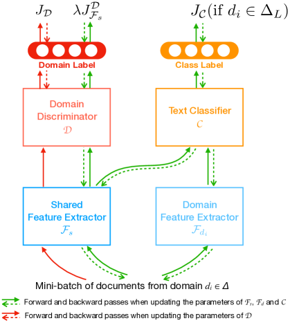
Figure 1: MAN for MDTC. The figure demonstrates the training on a mini-batch of data from one domain. One training iteration consists of one such mini-batch training from each domain. The parameters of ${\cal F}_{s},{\cal F}_{d},{\cal C}$ are updated together, and the training flows are illustrated by the green arrows. The parameters of ${\cal D}$ are updated separately, shown in red arrows. Solid lines indicate forward passes while dotted lines are backward passes. $J_{{\cal F}_{s}}^{\cal D}$ is the domain loss for ${\cal F}_{s}$, which is anticorrelated with $J_{\cal D}$ (e.g. $J_{{\cal F}_{s}}^{\cal D}=-J_{\cal D}$). (See §2,§3)

As shown in Figure 1, the Multinomial Adversarial Network (MAN) adopts the Shared-Private paradigm of Bousmalis et al. (2016) and consists of four components: a shared feature extractor ${\cal F}_{s}$, a domain feature extractor ${\cal F}_{d_{i}}$ for each labeled domain $d_{i}\in\Delta_{L}$, a text classifier ${\cal C}$, and finally a domain discriminator ${\cal D}$. The main idea of MAN is to explicitly model the domain-invariant features that are beneficial to the main classification task across all domains (i.e. shared features, extracted by ${\cal F}_{s}$), as well as the domain-specific features that mainly contribute to the classification in its own domain (domain features, extracted by ${\cal F}_{d}$). Here, the adversarial domain discriminator ${\cal D}$ has a multinomial output that takes a shared feature vector and predicts the likelihood of that sample coming from each domain. As seen in Figure 1 during the training flow of ${\cal F}_{s}$ (green arrows), ${\cal F}_{s}$ aims to confuse ${\cal D}$ by minimizing $J_{{\cal F}_{s}}^{\cal D}$ that is anticorrelated to $J_{\cal D}$ (detailed in §2.2), so that ${\cal D}$ cannot predict the domain of a sample given its shared features. The intuition is that if even a strong discriminator ${\cal D}$ cannot tell the domain of a sample from the extracted features, those features ${\cal F}_{s}$ learned are essentially domain invariant. By enforcing domain-invariant features to be learned by ${\cal F}_{s}$, when trained jointly via backpropagation, the set of domain features extractors ${\cal F}_{d}$ will each learn domain-specific features beneficial within its own domain.

The architecture of each component is relatively flexible, and can be decided by the practitioners to suit their particular classification tasks. For instance, the feature extractors can adopt the form of Convolutional Neural Nets (CNN), Recurrent Neural Nets (RNN), or a Multi-Layer Perceptron (MLP), depending on the input data (See §4). The input of MAN will also be dependent on the feature extractor choice. The output of a (shared/domain) feature extractor is a fixed-length vector, which is considered the (shared/domain) hidden features of some given input text. On the other hand, the outputs of ${\cal C}$ and ${\cal D}$ are label probabilities for class and domain prediction, respectively. For example, both ${\cal C}$ and ${\cal D}$ can be MLPs with a softmax layer on top. In §3, we provide alternative architectures for ${\cal D}$ and their mathematical implications. We now present detailed descriptions of the MAN training in §2.2 as well as the theoretical grounds in §3.

1:labeled corpus $\mathbb{X}$; unlabeled corpus $\mathbb{U}$; Hyperpamameter $\lambda>0$, $k\in\mathbb{N}$

2:repeat

3:   $\triangleright$ ${\cal D}$ iterations

4:   for $diter=1$ to $k$ do

5:      $l_{\cal D}=0$

6:      for all $d\in\Delta$ do$\triangleright$ For all $N$ domains

7:         Sample a mini-batch $\bm{x}\sim\mathbb{U}_{d}$

8:         $\bm{f}_{s}={\cal F}_{s}(\bm{x})$ $\triangleright$ Shared feature vector

9:         $l_{\cal D}\mathrel{+}=J_{\cal D}({\cal D}(\bm{f}_{s});d)$ $\triangleright$ Accumulate ${\cal D}$ loss       

10:      Update ${\cal D}$ parameters using $\nabla l_{\cal D}$    

11:   $\triangleright$ Main iteration

12:   $loss=0$

13:   for all $d\in\Delta_{L}$ do$\triangleright$ For all labeled domains

14:      Sample a mini-batch $(\bm{x},\bm{y})\sim\mathbb{X}_{d}$

15:      $\bm{f}_{s}={\cal F}_{s}(\bm{x})$

16:      $\bm{f}_{d}={\cal F}_{d}(\bm{x})$ $\triangleright$ Domain feature vector

17:      $loss\mathrel{+}=J_{\cal C}({\cal C}(\bm{f}_{s},\bm{f}_{d});\bm{y})$ $\triangleright$ Compute ${\cal C}$ loss    

18:   for all $d\in\Delta$ do$\triangleright$ For all $N$ domains

19:      Sample a mini-batch $\bm{x}\sim\mathbb{U}_{d}$

20:      $\bm{f}_{s}={\cal F}_{s}(\bm{x})$

21:      $loss\mathrel{+}=\lambda\cdot J_{{\cal F}_{s}}^{\cal D}({\cal D}(\bm{f}_{s});d)$ $\triangleright$ Domain loss of ${\cal F}_{s}$    

22:   Update ${\cal F}_{s}$, ${\cal F}_{d}$, ${\cal C}$ parameters using $\nabla loss$

23:until convergence

Algorithm 1 MAN Training

2.2 Training

Denote the annotated corpus in a labeled domain $d_{i}\in\Delta_{L}$ as $\mathbb{X}_{i}$; and $(x,y)\sim\mathbb{X}_{i}$ is a sample drawn from the labeled data in domain $d_{i}$, where $x$ is the input and $y$ is the task label. On the other hand, for any domain $d_{i^{\prime}}\in\Delta$, denote the unlabeled corpus as $\mathbb{U}_{i^{\prime}}$. Note for a labeled domain, one can use a separate unlabeled corpus or simply use the labeled data (or use both).

In Figure 1, the arrows illustrate the training flows of various components. Due to the adversarial nature of the domain discriminator ${\cal D}$, it is trained with a separate optimizer (red arrows), while the rest of the networks are updated with the main optimizer (green arrows). ${\cal C}$ is only trained on labeled domains, and it takes as input the concatenation of the shared and domain feature vectors. At test time for unlabeled domains with no ${\cal F}_{d}$, the domain features are set to the $\bf 0$ vector for ${\cal C}$’s input. On the contrary, ${\cal D}$ only takes the shared features as input, for both labeled and unlabeled domains. The MAN training is described in Algorithm 1.

In Algorithm 1, ${\cal L}_{\cal C}$ and ${\cal L}_{\cal D}$ are the loss functions of the text classifier ${\cal C}$ and the domain discriminator ${\cal D}$, respectively. As mentioned in  §2.1, ${\cal C}$ has a $softmax$ layer on top for classification. We hence adopt the canonical negative log-likelihood (NLL) loss:

$${\cal L}_{\cal C}(\hat{y},y)=-\log P(\hat{y}=y)$$ (1)

where $y$ is the true label and $\hat{y}$ is the $softmax$ predictions. For ${\cal D}$, we consider two variants of MAN. The first one is to use the NLL loss same as ${\cal C}$ which suits the classification task; while another option is to use the Least-Square (L2) loss that was shown to be able to alleviate the gradient vanishing problem when using the NLL loss in the adversarial setting Mao et al. (2017):

$${\cal L}^{NLL}_{\cal D}(\hat{d},d) =-\log P(\hat{d}=d)$$ (2)

$${\cal L}^{L2}_{\cal D}(\hat{d},d) =\sum_{i=1}^{N}(\hat{d}_{i}-\mathbbm{1}_{\{d=i\}})^{2}$$ (3)

where $d$ is the domain index of some sample and $\hat{d}$ is the prediction. Without loss of generality, we normalize $\hat{d}$ so that $\sum_{i=1}^{N}\hat{d}_{i}=1$ and $\forall i:\hat{d}_{i}\geq 0$.

Therefore, the objectives of ${\cal C}$ and ${\cal D}$ that we are minimizing are:

$$J_{\cal C} =\sum_{i=1}^{N}\mathop{{}\mathbb{E}}_{(x,y)\sim\mathbb{X}_{i}}\left[{\cal L}_{\cal C}({\cal C}({\cal F}_{s}(x),{\cal F}_{d}(x));y)\right]$$ (4)

$$J_{\cal D} =\sum_{i=1}^{N}\mathop{{}\mathbb{E}}_{x\sim\mathbb{U}_{i}}\left[{\cal L}_{\cal D}({\cal D}({\cal F}_{s}(x));d)\right]$$ (5)

For the feature extractors, the training of domain feature extractors is straightforward, as their sole objective is to help ${\cal C}$ perform better within their own domain. Hence, $J_{{\cal F}_{d}}=J_{\cal C}$ for any domain $d$. Finally, the shared feature extractor ${\cal F}_{s}$ has two objectives: to help ${\cal C}$ achieve higher accuracy, and to make the feature distribution invariant across all domains. It thus leads to the following bipartite loss:

$$J_{{\cal F}_{s}}=J_{{\cal F}_{s}}^{\cal C}+\lambda\cdot J_{{\cal F}_{s}}^{\cal D}$$

where $\lambda$ is a hyperparameter balancing the two parts. $J_{{\cal F}_{s}}^{\cal D}$ is the domain loss of ${\cal F}_{s}$ anticorrelated to $J_{\cal D}$:

$$(NLL)J_{{\cal F}_{s}}^{\cal D} =-J_{\cal D}$$ (6)

$$(L2)J_{{\cal F}_{s}}^{\cal D} =\sum_{i=1}^{N}\mathop{{}\mathbb{E}}_{x\sim\mathbb{U}_{i}}\left[\sum_{j=1}^{N}({\cal D}_{j}({\cal F}_{s}(x))-\frac{1}{N})^{2}\right]$$ (7)

If ${\cal D}$ adopts the NLL loss (6), the domain loss is simply $-J_{\cal D}$. For the L2 loss (7), $J_{{\cal F}_{s}}^{\cal D}$ intuitively translates to pushing ${\cal D}$ to make random predictions. See §3 for theoretical justifications.

3 Theories of Multinomial Adversarial Networks

The binomial adversarial nets are known to have theoretical connections to the minimization of various f-divergences between two distributions Nowozin et al. (2016). However, for adversarial training among multiple distributions, despite similar idea has been empirically experimented Liu et al. (2017), no theoretical justifications have been provided to our best knowledge.

In this section, we present a theoretical analysis showing the validity of MAN. In particular, we show that MAN’s objective is equivalent to minimizing the total f-divergence between each of the shared feature distributions of the $N$ domains, and the centroid of the $N$ distributions. The choice of loss function will determine which specific f-divergence is minimized. Furthermore, with adequate model capacity, MAN achieves its optimum for either loss function if and only if all $N$ shared feature distributions are identical, hence learning an invariant feature space across all domains.

First consider the distribution of the shared features ${\bf f}$ for instances in each domain $d_{i}\in\Delta$:

$$P_{i}({\bf f})\triangleq P({\bf f}={\cal F}_{s}(x)|x\in d_{i})$$ (8)

Combining (5) with the two loss functions (2), (3), the objective of ${\cal D}$ can be written as:

$$J^{NLL}_{\cal D} =-\sum_{i=1}^{N}\mathop{{}\mathbb{E}}_{{\bf f}\sim P_{i}}\left[\log{\cal D}_{i}({\bf f})\right]$$ (9)

$$J^{L2}_{\cal D} =\sum_{i=1}^{N}\mathop{{}\mathbb{E}}_{{\bf f}\sim P_{i}}\left[\sum_{j=1}^{N}({\cal D}_{j}({\bf f})-\mathbbm{1}_{\{i=j\}})^{2}\right]$$ (10)

where ${\cal D}_{i}({\bf f})$ is the $i$-th dimension of ${\cal D}$’s (normalized) output vector, which conceptually corresponds to the probability of ${\cal D}$ predicting that ${\bf f}$ is from domain $d_{i}$.

We first derive the optimal ${\cal D}$ for any fixed ${\cal F}_{s}$.

Lemma 1.

For any fixed ${\cal F}_{s}$, with either NLL or L2 loss, the optimum domain discriminator ${\cal D}^{*}$ is:

$${\cal D}_{i}^{*}({\bf f})=\frac{P_{i}({\bf f})}{\sum_{j=1}^{N}P_{j}({\bf f})}$$ (11)

The proof involves an application of the Lagrangian Multiplier to solve the minimum value of $J_{\cal D}$, and the details can be found in the Appendix. We then have the following main theorems for the domain loss for ${\cal F}_{s}$:

Theorem 1.

Let $\overline{P}=\frac{\sum_{i=1}^{N}P_{i}}{N}$. When ${\cal D}$ is trained to its optimality, if ${\cal D}$ adopts the NLL loss:

$$J_{{\cal F}_{s}}^{{\cal D}} =-\min_{\theta_{\cal D}}J_{{\cal D}}=-J_{{\cal D}^{*}}$$

$$=-N\log N+N\cdot\mathit{JSD}(P_{1},P_{2},\dots,P_{N})$$

$$=-N\log N+\sum_{i=1}^{N}\mathit{KL}(P_{i}\|\overline{P})$$

where $\mathit{JSD}(\cdot)$ is the generalized Jensen-Shannon Divergence Lin (1991) among multiple distributions, defined as the average Kullback-Leibler divergence of each $P_{i}$ to the centroid $\overline{P}$ Aslam and Pavlu (2007).

Theorem 2.

If ${\cal D}$ uses the L2 loss:

$$J_{{\cal F}_{s}}^{{\cal D}} =\sum_{i=1}^{N}\mathop{{}\mathbb{E}}_{{\bf f}\sim P_{i}}\left[\sum_{j=1}^{N}({\cal D}^{*}_{j}({\bf f})-\frac{1}{N})^{2}\right]$$

$$=\frac{1}{N}\sum_{i=1}^{N}\chi_{\mathit{Neyman}}^{2}(P_{i}\|\overline{P})$$

where $\chi_{\mathit{Neyman}}^{2}(\cdot\|\cdot)$ is the Neyman $\chi^{2}$ divergence Nielsen and Nock (2014). The proof of both theorems can be found in the Appendix.

Consequently, by the non-negativity and joint convexity of the f-divergence Csiszar and Korner (1982), we have:

Corollary 1.

The optimum of $J_{{\cal F}_{s}}^{\cal D}$ is $-N\log N$ when using NLL loss, and $0$ for the L2 loss. The optimum value above is achieved if and only if $P_{1}=P_{2}=\dots=P_{N}=\overline{P}$ for either loss.

Therefore, the loss of ${\cal F}_{s}$ can be interpreted as simultaneously minimizing the classification loss $J_{\cal C}$ as well as the divergence among feature distributions of all domains. It can thus learn a shared feature mapping that are invariant across domains upon successful training while being beneficial to the main classification task.

4 Experiments

4.1 Multi-Domain Text Classification

In this experiment, we compare MAN to state-of-the-art MDTC systems, on the multi-domain Amazon review dataset Blitzer et al. (2007), which is one of the most widely used MDTC datasets. Note that this dataset was already preprocessed into a bag of features (unigrams and bigrams), losing all word order information. This prohibits the usage of CNNs or RNNs as feature extractors, limiting the potential performance of the system. Nonetheless, we adopt the same dataset for fair comparison and employ a MLP as our feature extractor. In particular, we take the 5000 most frequent features and represent each review as a 5000d feature vector, where feature values are raw counts of the features. Our MLP feature extractor would then have an input size of 5000 in order to process the reviews.

The Amazon dataset contains 2000 samples for each of the four domains: book, DVD, electronics, and kitchen, with binary labels (positive, negative). Following Wu and Huang (2015), we conduct 5-way cross validation. Three out of the five folds are treated as training set, one serves as the validation set, while the remaining being the test set. The 5-fold average test accuracy is reported.

[t] Book DVD Elec. Kit. Avg. Domain-Specific Models Only LS 77.80 77.88 81.63 84.33 80.41 SVM 78.56 78.66 83.03 84.74 81.25 LR 79.73 80.14 84.54 86.10 82.63 MLP 81.70 81.65 85.45 85.95 83.69 Shared Model Only LS 78.40 79.76 84.67 85.73 82.14 SVM 79.16 80.97 85.15 86.06 82.83 LR 80.05 81.88 85.19 86.56 83.42 MLP 82.40 82.15 85.90 88.20 84.66 MAN-L2-MLP 82.05 83.45 86.45 88.85 85.20 MAN-NLL-MLP 81.85 83.10 85.75 89.10 84.95 Shared-Private Models RMTL¹ 81.33 82.18 85.49 87.02 84.01 MTLGraph² 79.66 81.84 83.69 87.06 83.06 CMSC-LS³ 82.10 82.40 86.12 87.56 84.55 CMSC-SVM³ 82.26 83.48 86.76 88.20 85.18 CMSC-LR³ 81.81 83.73 86.67 88.23 85.11 SP-MLP 82.00 84.05 86.85 87.30 85.05 MAN-L2-SP-MLP 82.46 ($\pm 0.25$) 83.98 ($\pm 0.17$) 87.22*
($\pm 0.04$) 88.53 ($\pm 0.19$) 85.55* ($\pm 0.07$) MAN-NLL-SP-MLP 82.98*
($\pm 0.28$) 84.03 ($\pm 0.16$) 87.06 ($\pm 0.23$) 88.57*
($\pm 0.15$) 85.66*
($\pm 0.14$)

• Evgeniou and Pontil (2004)

• Zhou et al. (2011)

• Wu and Huang (2015)

Table 1: MDTC results on the Amazon dataset. Models in bold are ours while the performance of the rest is taken from Wu and Huang (2015). Numbers in parentheses indicate standard errors, calculated based on 5 runs. Bold numbers indicate the highest performance in each domain, and $*$ shows statistical significance ($p<0.05$) over CMSC under a one-sample T-Test.

Table 1 shows the main results. Three types of models are shown: Domain-Specific Models Only, where only in-domain models are trained; Shared Model Only, where a single model is trained with all data; and Shared-Private Models, a combination of the previous two. Within each category, various architectures are examined, such as Least Square (LS), SVM, and Logistic Regression (LR). As explained before, we use MLP as our feature extractors for all our models (bold ones). Among our models, the ones with the MAN prefix use adversarial training, and MAN-L2 and MAN-NLL indicate the L2 loss and NLL loss MAN, respectively.

From Table 1, we can see that by adopting modern deep neural networks, our methods achieve superior performance within the first two model categories even without adversarial training. This is corroborated by the fact that our SP-MLP model performs comparably to CMSC, while the latter relies on external resources such as sentiment lexica. Moreover, when our multinomial adversarial nets are introduced, further improvement is observed. With both loss functions, MAN outperforms all Shared-Private baseline systems on each domain, and achieves statistically significantly higher overall performance. For our MAN-SP models, we provide the mean accuracy as well as the standard errors over five runs, to illustrate the performance variance and conduct significance test. It can be seen that MAN’s performance is relatively stable, and consistently outperforms CMSC.

4.2 Experiments for Unlabeled Domains

As CMSC requires labeled data for each domain, their experiments were naturally designed this way. In reality, however, many domains may not have any annotated corpora available. It is therefore also important to look at the performance in these unlabeled domains for a MDTC system. Fortunately, as depicted before, MAN’s adversarial training only utilizes unlabeled data from each domain to learn the domain-invariant features, and can thus be used on unlabeled domains as well. During testing, only the shared feature vector is fed into ${\cal C}$, while the domain feature vector is set to $\bf 0$.

Target Domain	Book	DVD	Elec.	Kit.	Avg.
MLP	76.55	75.88	84.60	85.45	80.46
mSDA1	76.98	78.61	81.98	84.26	80.46
DANN2	77.89	78.86	84.91	86.39	82.01
MDAN (H-MAX)3	78.45	77.97	84.83	85.80	81.76
MDAN (S-MAX)3	78.63	80.65	85.34	86.26	82.72
MAN-L2-SP-MLP	78.45	81.57	83.37	85.57	82.24
MAN-NLL-SP-MLP	77.78	82.74	83.75	86.41	82.67

• Chen et al. (2012)

• Ganin et al. (2016)

• Zhao et al. (2017)

Table 2: Results on unlabeled domains. Models in bold are our models while the rest is taken from Zhao et al. (2017). Highest domain performance is shown in bold.

In order to validate MAN’s effectiveness, we compare to state-of-the-art multi-source domain adaptation (MS-DA) methods (See §5). Compared to standard domain adaptation methods with one source and one target domain, MS-DA allows the adaptation from multiple source domains to a single target domain. Analogically, MDTC can be viewed as multi-source multi-target domain adaptation, which is superior when multiple target domains exist. With multiple target domains, MS-DA will need to treat each one as an independent task, which is more expensive and cannot utilize the unlabeled data in other target domains.

In this work, we compare MAN with one recent MS-DA method, MDAN Zhao et al. (2017). Their experiments only have one target domain to suit their approach, and we follow this setting for fair comparison. However, it is worth noting that MAN is designed for the MDTC setting, and can deal with multiple target domains at the same time, which can potentially improve the performance by taking advantage of more unlabeled data from multiple target domains during adversarial training. We adopt the same setting as Zhao et al. (2017), which is based on the same multi-domain Amazon review dataset. Each of the four domains in the dataset is treated as the target domain in four separate experiments, while the remaining three are used as source domains.

	books	elec.	dvd	kitchen	apparel	camera	health	music	toys	video	baby	magaz.	softw.	sports	IMDb	MR	Avg.
Domain-Specific Models Only
BiLSTM	81.0	78.5	80.5	81.2	86.0	86.0	78.7	77.2	84.7	83.7	83.5	91.5	85.7	84.0	85.0	74.7	82.6
CNN	85.3	87.8	76.3	84.5	86.3	89.0	87.5	81.5	87.0	82.3	82.5	86.8	87.5	85.3	83.3	75.5	84.3
Shared Model Only
FS-MTL	82.5	85.7	83.5	86.0	84.5	86.5	88.0	81.2	84.5	83.7	88.0	92.5	86.2	85.5	82.5	74.7	84.7
MAN-L2-CNN	88.3	88.3	87.8	88.5	85.3	90.5	90.8	85.3	89.5	89.0	89.5	91.3	88.3	89.5	88.5	73.8	87.7
MAN-NLL-CNN	88.0	87.8	87.3	88.5	86.3	90.8	89.8	84.8	89.3	89.3	87.8	91.8	90.0	90.3	87.3	73.5	87.6
Shared-Private Models
ASP-MTL	84.0	86.8	85.5	86.2	87.0	89.2	88.2	82.5	88.0	84.5	88.2	92.2	87.2	85.7	85.5	76.7	86.1
MAN-L2-SP-CNN	87.6*	87.4	88.1*	89.8*	87.6	91.4*	89.8*	85.9*	90.0*	89.5*	90.0	92.5	90.4*	89.0*	86.6	76.1	88.2*
	$(0.2)$	$(1.0)$	$(0.4)$	$(0.4)$	$(0.7)$	$(0.4)$	$(0.3)$	$(0.1)$	$(0.1)$	$(0.2)$	$(0.6)$	$(0.5)$	$(0.4)$	$(0.4)$	$(0.5)$	$(0.5)$	$(0.1)$
MAN-NLL-SP-CNN	86.8*	88.8	88.6*	89.9*	87.6	90.7	89.4	85.5*	90.4*	89.6*	90.2	92.9	90.9*	89.0*	87.0*	76.7	88.4*
	$(0.4)$	$(0.6)$	$(0.4)$	$(0.4)$	$(0.4)$	$(0.4)$	$(0.3)$	$(0.1)$	$(0.2)$	$(0.3)$	$(0.6)$	$(0.4)$	$(0.7)$	$(0.2)$	$(0.1)$	$(0.8)$	$(0.1)$

Table 3: Results on the FDU-MTL dataset. Bolded models are ours, while the rest is from Liu et al. (2017). Highest performance is each domain is highlighted. For our full MAN models, standard errors are shown in parenthese and statistical significance ($p<0.01$) over ASP-MTL is indicated by *.

In Table 2, the target domain is shown on top, and the test set accuracy is reported for various systems. It shows that MAN outperforms several baseline systems, such as a MLP trained on the source-domains, as well as single-source domain adaptation methods such as mSDA Chen et al. (2012) and DANN Ganin et al. (2016), where the training data in the multiple source domains are combined and viewed as a single domain. Finally, when compared to MDAN, MAN and MDAN each achieves higher accuracy on two out of the four target domains, and the average accuracy of MAN is similar to MDAN. Therefore, MAN achieves competitive performance for the domains without annotated corpus. Nevertheless, unlike MS-DA methods, MAN can handle multiple target domains at one time.

4.3 Experiments on the MTL Dataset

To make fair comparisons, the previous experiments follow the standard settings in the literature, where the widely adopted Amazon review dataset is used. However, this dataset has a few limitations: First, it has only four domains. In addition, the reviews are already tokenized and converted to a bag of features consisting of unigrams and bigrams. Raw review texts are hence not available in this dataset, making it impossible to use certain modern neural architectures such as CNNs and RNNs. To provide more insights on how well MAN work with other feature extractor architectures, we provide a third set of experiments on the FDU-MTL dataset Liu et al. (2017). The dataset is created as a multi-task learning dataset with 16 tasks, where each task is essentially a different domain of reviews. It has 14 Amazon domains: books, electronics, DVD, kitchen, apparel, camera, health, music, toys, video, baby, magazine, software, and sports, in addition to two movies review domains from the IMDb and the MR dataset. Each domain has a development set of 200 samples, and a test set of 400 samples. The amount of training and unlabeled data vary across domains but are roughly 1400 and 2000, respectively.

We compare MAN with ASP-MTL Liu et al. (2017) on this FDU-MTL dataset. ASP-MTL also adopts adversarial training for learning a shared feature space, and can be viewed as a special case of MAN when adopting the NLL loss (MAN-NLL). Furthermore, while Liu et al. (2017) do not provide any theoretically justifications, we in §3 prove the validity of MAN for not only the NLL loss, but an additional L2 loss. Besides the theoretical superiority, we in this section show that MAN also substantially outperforms ASP-MTL in practice due to the feature extractor choice.

In particular, Liu et al. (2017) choose LSTM as their feature extractor, yet we found CNN Kim (2014) to achieve much better accuracy while being $\sim 10$ times faster. Indeed, as shown in Table 3, with or without adversarial training, our CNN models outperform LSTM ones by a large margin. When MAN is introduced, we attain the state-of-the-art performance on every domain with a 88.4% overall accuracy, surpassing ASP-MTL by a significant margin of 2.3%.

We hypothesize the reason LSTM performs much inferior to CNN is attributed to the lack of attention mechanism. In ASP-MTL, only the last hidden unit is taken as the extracted features. While LSTM is effective for representing the context for each token, it might not be powerful enough for directly encoding the entire document Bahdanau et al. (2015). Therefore, various attention mechanisms have been introduced on top of the vanilla LSTM to select words (and contexts) most relevant for making the predictions. In our preliminary experiments, we find that Bi-directional LSTM with the dot-product attention Luong et al. (2015) yields better performance than the vanilla LSTM in ASP-MTL. However, it still does not outperform CNN and is much slower. As a result, we conclude that, for text classification tasks, CNN is both effective and efficient in extracting local and higher-level features for making a single categorization.

Finally, we observe that MAN-NLL achieves slightly higher overall performance compared to MAN-L2, providing evidence for the claim in a recent study Lucic et al. (2017) that the original GAN loss (NLL) may not be inherently inferior. Moreover, the two variants excel in different domains, suggesting the possibility of further performance gain when using ensemble.

5 Related Work

Multi-Domain Text Classification

The MDTC task was first examined by Li and Zong (2008), who proposed to fusion the training data from multiple domains either on the feature level or the classifier level. The prior art of MDTC Wu and Huang (2015) decomposes the text classifier into a general one and a set of domain-specific ones. However, the general classifier is learned by parameter sharing and domain-specific knowledge may sneak into it. They also require external resources to help improve accuracy and compute domain similarities.

Domain Adaptation

Domain Adaptation attempts to transfer the knowledge from a source domain to a target one, and the traditional form is the single-source, single-target (SS,ST) adaptation Blitzer et al. (2006). Another variant is the SS,MT adaptation Yang and Eisenstein (2015), which tries to simultaneously transfer the knowledge to multiple target domains from a single source. However, it cannot fully take advantage the training data if it comes from multiple source domains. MS,ST adaptation Mansour et al. (2009); Zhao et al. (2017) can deal with multiple source domains but only transfers to a single target domain. Therefore, when multiple target domains exist, they need to treat them as independent problems, which is more expensive and cannot utilize the additional unlabeled data in these domains. Finally, MDTC can be viewed as MS,MT adaptation, which is arguably more general and realistic.

Adversarial Networks

The idea of adversarial networks was proposed by Goodfellow et al. (2014) for image generation, and has been applied to various NLP tasks as well Chen et al. (2016); Li et al. (2017). Ganin et al. (2016) first used it for the SS,ST domain adaptation followed by many others. Bousmalis et al. (2016) utilized adversarial training in a shared-private model for domain adaptation to learn domain-invariant features, but still focused on the SS,ST setting. Finally, the idea of using adversarial nets to discriminate over multiple distributions was empirically explored by a very recent work Liu et al. (2017) under the multi-task learning setting, and can be considered as a special case of our MAN framework with the NLL domain loss. Nevertheless, we propose a more general framework with alternative architectures for the adversarial component, and for the first time provide theoretical justifications for the multinomial adversarial nets. Moreover, Liu et al. (2017) used LSTM without attention as their feature extractor, which we found to perform sub-optimal in the experiments. We instead chose Convolutional Neural Nets as our feature extractor that achieves higher accuracy while running an order of magnitude faster (See §4.3).

6 Conclusion

In this work, we propose a family of Multinomial Adversarial Networks (MAN) that generalize the traditional binomial adversarial nets in the sense that MAN can simultaneously minimize the difference among multiple probability distributions instead of two. We provide theoretical justifications for two instances of MAN, MAN-NLL and MAN-L2, showing they are minimizers of two different f-divergence metrics among multiple distributions, respectively. This indicates MAN can be used to make multiple distributions indistinguishable from one another. It can hence be applied to a variety of tasks, similar to the versatile binomial adversarial nets, which have been used in many areas for making two distributions alike.

We in this paper design a MAN model for the MDTC task, following the shared-private paradigm that has a shared feature extractor to learn domain-invariant features and domain feature extractors to learn domain-specific ones. MAN is used to enforce the shared feature extractor to learn only domain-invariant knowledge, by resorting to MAN’s power of making indistinguishable the shared feature distributions of samples from each domain. We conduct extensive experiments, demonstrating our MAN model outperforms the prior art systems in MDTC, and achieves state-of-the-art performance on domains without labeled data when compared to multi-source domain adaptation methods.

Appendix A Proofs

A.1 Proofs for MAN-NLL

Assume we have $N$ domains, consider the distribution of the shared features ${\cal F}_{s}$ for instances in each domain $d_{i}$:

$$P_{i}({\bf f})\triangleq P({\bf f}={\cal F}_{s}(x)|x\in d_{i})$$

The objective that ${\cal D}$ attempts to minimize is:

$$J_{\cal D}=-\sum_{i=1}^{N}\mathop{{}\mathbb{E}}_{{\bf f}\sim P_{i}}\left[\log{\cal D}_{i}({\bf f})\right]$$ (12)

where ${\cal D}_{i}({\bf f})$ is the $i$-th dimension of ${\cal D}$’s output vector, which conceptually corresponds to the softmax probability of ${\cal D}$ predicting that ${\bf f}$ is from domain $d_{i}$. We therefore have property that for any ${\bf f}$:

$$\sum_{i=1}^{N}{\cal D}_{i}({\bf f})=1$$ (13)

Lemma 2.

For any fixed ${\cal F}_{s}$, the optimum domain discriminator ${\cal D}^{*}$ is:

$${\cal D}_{i}^{*}({\bf f})=\frac{P_{i}({\bf f})}{\sum_{j=1}^{N}P_{j}({\bf f})}$$ (14)

Proof.

For a fixed ${\cal F}_{s}$, the optimum

$${\cal D}^{*}=\operatorname*{arg\,min}_{\cal D}J_{\cal D} =\operatorname*{arg\,min}_{\cal D}-\sum_{i=1}^{N}\mathop{{}\mathbb{E}}_{{\bf f}\sim P_{i}}\left[\log{\cal D}_{i}({\bf f})\right]$$

$$=\operatorname*{arg\,max}_{\cal D}\sum_{i=1}^{N}\int_{\bf f}P_{i}({\bf f})\log{\cal D}_{i}({\bf f})d{\bf f}$$

$$=\operatorname*{arg\,max}_{\cal D}\int_{\bf f}\sum_{i=1}^{N}P_{i}({\bf f})\log{\cal D}_{i}({\bf f})d{\bf f}$$

We employ the Lagrangian Multiplier to derive $\operatorname*{arg\,max}_{\cal D}\sum_{i=1}^{N}P_{i}({\bf f})\log{\cal D}_{i}({\bf f})$ under the constraint of (13). Let

$$L({\cal D}_{1},\dots,{\cal D}_{N},\lambda) =\sum_{i=1}^{N}P_{i}\log{\cal D}_{i}-\lambda(\sum_{i=1}^{N}{\cal D}_{i}-1)$$

Let $\nabla L=0$:

$$\begin{cases}\nabla_{{\cal D}_{i}}\sum_{j=1}^{N}P_{j}\log{\cal D}_{j}=\lambda\nabla_{{\cal D}_{i}}(\sum_{j=1}^{N}{\cal D}_{j}-1)&(\forall i)\\ \sum_{i=1}^{N}{\cal D}_{i}-1=0\end{cases}$$

Solving the two equations, we have:

$${\cal D}_{i}^{*}({\bf f})=\frac{P_{i}({\bf f})}{\sum_{j=1}^{N}P_{j}({\bf f})}$$

∎

On the other hand, the loss function of the shared feature extractor ${\cal F}_{s}$ consists of two additive components, the loss from the text classifier ${\cal C}$, and the loss from the domain discriminator ${\cal D}$:

$$J_{{\cal F}_{s}}=J_{{\cal F}_{s}}^{{\cal C}}+\lambda J_{{\cal F}_{s}}^{{\cal D}}\triangleq J_{\cal C}-\lambda J_{\cal D}$$ (15)

We have the following theorem for the domain loss for ${\cal F}_{s}$:

Theorem 3.

When ${\cal D}$ is trained to its optimality:

$$J_{{\cal F}_{s}}^{D}=-J_{{\cal D}^{*}}=-N\log N+N\cdot\mathit{JSD}(P_{1},P_{2},\dots,P_{N})$$ (16)

where $\mathit{JSD}(\cdot)$ is the generalized Jensen-Shannon Divergence Lin (1991) among multiple distributions.

Proof.

Let $\overline{P}=\frac{\sum_{i=1}^{N}P_{i}}{N}$.

There are two equivalent definitions of the generalized Jensen-Shannon divergence: the original definition based on Shannon entropy Lin (1991), and a reshaped one expressed as the average Kullback-Leibler divergence of each $P_{i}$ to the centroid $\overline{P}$ Aslam and Pavlu (2007). We adopt the latter one here:

$$\mathit{JSD}(P_{1},P_{2},\dots,P_{N})\triangleq\frac{1}{N}\sum_{i=1}^{N}\mathit{KL}(P_{i}\|\overline{P})=\frac{1}{N}\sum_{i=1}^{N}\mathop{{}\mathbb{E}}_{{\bf f}\sim P_{i}}\left[\log\frac{P_{i}({\bf f})}{\overline{P}({\bf f})}\right]$$ (17)

Now substituting ${\cal D}^{*}$ into $J_{{\cal F}_{s}}^{\cal D}$:

$$J_{{\cal F}_{s}}^{{\cal D}}=-J_{{\cal D}^{*}} =\sum_{i=1}^{N}\mathop{{}\mathbb{E}}_{{\bf f}\sim P_{i}}\left[\log{\cal D}^{*}_{i}({\bf f})\right]$$

$$=\sum_{i=1}^{N}\mathop{{}\mathbb{E}}_{{\bf f}\sim P_{i}}\left[\log\frac{P_{i}({\bf f})}{\sum_{j=1}^{N}P_{j}({\bf f})}\right]$$

$$=-N\log N+\sum_{i=1}^{N}\mathop{{}\mathbb{E}}_{{\bf f}\sim P_{i}}\left[\log\frac{P_{i}({\bf f})}{\sum_{j=1}^{N}P_{j}({\bf f})}+\log N\right]$$

$$=-N\log N+\sum_{i=1}^{N}\mathop{{}\mathbb{E}}_{{\bf f}\sim P_{i}}\left[\log\frac{P_{i}({\bf f})}{\frac{\sum_{j=1}^{N}P_{j}({\bf f})}{N}}\right]$$

$$=-N\log N+\sum_{i=1}^{N}\mathop{{}\mathbb{E}}_{{\bf f}\sim P_{i}}\left[\log\frac{P_{i}({\bf f})}{\overline{P}}\right]$$

$$=-N\log N+\sum_{i=1}^{N}\mathit{KL}(P_{i}\|\overline{P})$$

$$=-N\log N+N\cdot\mathit{JSD}(P_{1},P_{2},\dots,P_{N})$$

∎

Consequently, by the non-negativity of $\mathit{JSD}$ Lin (1991), we have the following corollary:

Corollary 2.

The optimum of $J_{{\cal F}_{s}}^{\cal D}$ is $-N\log N$, and is achieved if and only if $P_{1}=P_{2}=\dots=P_{N}=\overline{P}$.

A.2 Proofs for MAN-L2

The proof is similar for MAN with the L2 loss. The loss function used by ${\cal D}$ is, for a sample from domain $d_{i}$ with shared feature vector ${\bf f}$:

$${\cal L}_{\cal D}({\cal D}({\bf f}),i)=\sum_{j=1}^{N}({\cal D}_{j}({\bf f})-\mathbbm{1}_{\{i=j\}})^{2}$$ (18)

So the objective that ${\cal D}$ minimizes is:

$$J_{\cal D}=\sum_{i=1}^{N}\mathop{{}\mathbb{E}}_{{\bf f}\sim P_{i}}\left[\sum_{j=1}^{N}({\cal D}_{j}({\bf f})-\mathbbm{1}_{\{i=j\}})^{2}\right]$$ (19)

For simplicity, we further constrain ${\cal D}$’s outputs to be on a simplex:

$$\sum_{i=1}^{N}{\cal D}_{i}({\bf f})=1\quad(\forall{\bf f})$$ (20)

Lemma 3.

For any fixed ${\cal F}_{s}$, the optimum domain discriminator ${\cal D}^{*}$ is:

$${\cal D}_{i}^{*}({\bf f})=\frac{P_{i}({\bf f})}{\sum_{j=1}^{N}P_{j}({\bf f})}$$ (21)

Proof.

For a fixed ${\cal F}_{s}$, the optimum

$${\cal D}^{*}=\operatorname*{arg\,min}_{\cal D}J_{\cal D} =\operatorname*{arg\,min}_{\cal D}\sum_{i=1}^{N}\mathop{{}\mathbb{E}}_{{\bf f}\sim P_{i}}\left[{\cal L}_{\cal D}({\cal D}({\bf f}),i)\right]$$

$$=\operatorname*{arg\,min}_{\cal D}\sum_{i=1}^{N}\int_{\bf f}P_{i}({\bf f}){\cal L}_{\cal D}({\cal D}({\bf f}),i)d{\bf f}$$

$$=\operatorname*{arg\,min}_{\cal D}\int_{\bf f}\sum_{i=1}^{N}P_{i}({\bf f})\sum_{j=1}^{N}({\cal D}_{j}({\bf f})-\mathbbm{1}_{\{i=j\}})^{2}d{\bf f}$$

Similar to MAN-NLL, we employ the Lagrangian Multiplier to derive $\operatorname*{arg\,max}_{\cal D}\sum_{i=1}^{N}P_{i}({\bf f})\sum_{j=1}^{N}({\cal D}_{j}({\bf f})-\mathbbm{1}_{\{i=j\}})^{2}$ under the constraint of (20). Let $\nabla L=0$:

$$\begin{cases}2((\sum_{j=1}^{N}P_{j}){\cal D}_{i}-P_{i})=\lambda&(\forall i)\\ \sum_{i=1}^{N}{\cal D}_{i}-1=0\end{cases}$$

Solving the two equations, we have $\lambda=0$ and:

$${\cal D}_{i}^{*}({\bf f})=\frac{P_{i}({\bf f})}{\sum_{j=1}^{N}P_{j}({\bf f})}$$

∎

For the domain loss of ${\cal F}_{s}$:

Theorem 4.

Let $\overline{P}=\frac{\sum_{i=1}^{N}P_{i}}{N}$. When ${\cal D}$ is trained to its optimality:

$$J_{{\cal F}_{s}}^{{\cal D}} =\sum_{i=1}^{N}\mathop{{}\mathbb{E}}_{{\bf f}\sim P_{i}}\left[\sum_{j=1}^{N}(D_{j}({\bf f})-\frac{1}{N})^{2}\right]$$

$$=\frac{1}{N}\sum_{i=1}^{N}\chi_{\mathit{Neyman}}^{2}(P_{i}\|\overline{P})$$ (22)

where $\chi_{\mathit{Neyman}}^{2}(\cdot\|\cdot)$ is the Neyman $\chi^{2}$ divergence Nielsen and Nock (2014).

Proof.

Substituting ${\cal D}^{*}$ into ${\cal L}_{{\cal F}_{s}}^{\cal D}$:

$$J_{{\cal F}_{s}}^{{\cal D}} =\sum_{i=1}^{N}\mathop{{}\mathbb{E}}_{{\bf f}\sim P_{i}}\left[\sum_{j=1}^{N}(D^{*}_{j}({\bf f})-\frac{1}{N})^{2}\right]$$

$$=\sum_{i=1}^{N}\int_{\bf f}P_{i}\sum_{j=1}^{N}(\frac{P_{j}}{N\overline{P}}-\frac{1}{N})^{2}d{\bf f}$$

$$=\int_{\bf f}\sum_{i=1}^{N}\sum_{j=1}^{N}P_{i}(\frac{P_{j}}{N\overline{P}}-\frac{1}{N})^{2}d{\bf f}$$

$$=\frac{1}{N^{2}}\sum_{j=1}^{N}\int_{\bf f}\sum_{i=1}^{N}P_{i}(\frac{P_{j}}{\overline{P}}-1)^{2}d{\bf f}$$

$$=\frac{1}{N^{2}}\sum_{j=1}^{N}\int_{\bf f}N\overline{P}(\frac{P_{j}}{\overline{P}}-1)^{2}d{\bf f}$$

$$=\frac{1}{N}\sum_{j=1}^{N}\int_{\bf f}\frac{(P_{j}-\overline{P})^{2}}{\overline{P}}d{\bf f}$$

$$=\frac{1}{N}\sum_{i=1}^{N}\chi_{\mathit{Neyman}}^{2}(P_{i}\|\overline{P})$$

∎

Finally, by the joint convexity of f-divergence, we have the following corollary:

Corollary 3.

$${\cal L}_{{\cal F}_{s}}^{\cal D} =\frac{1}{N}\sum_{i=1}^{N}\chi_{\mathit{Neyman}}^{2}(P_{i}\|\overline{P})$$

$$\geq\chi_{\mathit{Neyman}}^{2}(\frac{1}{N}\sum_{i=1}^{N}P_{i}\|\frac{1}{N}\sum_{i=1}^{N}\overline{P})$$

$$=\chi_{\mathit{Neyman}}^{2}(\overline{P}\|\overline{P})=0$$

and the equality is attained if and only if $P_{1}=P_{2}=\dots=P_{N}=\overline{P}$.

Appendix B Implementation Details

For all three of our experiments, we use $\lambda=0.05$ and $k=5$ (See Algorithm 1). For both optimizers, Adam Kingma and Ba (2015) is used with learning rate $0.0001$. The size of the shared feature vector is set to $128$ while that of the domain feature vector is $64$. Dropout of $p=0.4$ is used in all components. ${\cal C}$ and ${\cal D}$ each has one hidden layer of the same size as their input ($128+64$ for ${\cal C}$ and $128$ for ${\cal D}$). ReLU is used as the activation function. Batch normalization Ioffe and Szegedy (2015) is used in both ${\cal C}$ and ${\cal D}$ but not $\mathcal{F}$. We use a batch size of 8.

For our first two experiments on the Amazon review dataset, the MLP feature extractor is used. As described in the paper, it has an input size of 5000. Two hidden layers are used, with size $1000$ and $500$, respectively.

For the CNN feature extractor used in the FDU-MTL experiment, a single convolution layer is used. The kernel sizes are 3, 4, and 5, and the number of kernels are 200. The convolution layers take as input the 100d word embeddings of each word in the input sequence. We use word2vec word embeddings Mikolov et al. (2013) trained on a bunch of unlabeled raw Amazon reviews Blitzer et al. (2007). After convolution, the outputs go through a ReLU layer before fed into a max pooling layer. The pooled output is then fed into a single fully connected layer to be converted into a feature vector of size either 128 or 64. More details of using CNN for text classification can be found in the original paper Kim (2014). MAN is implemented using PyTorch Paszke et al. (2017).

References

- Ali and Silvey (1966) S. M. Ali and S. D. Silvey. 1966. A general class of coefficients of divergence of one distribution from another. Journal of the Royal Statistical Society. Series B (Methodological) 28(1):131–142. http://www.jstor.org/stable/2984279.
- Aslam and Pavlu (2007) Javed A. Aslam and Virgil Pavlu. 2007. Query Hardness Estimation Using Jensen-Shannon Divergence Among Multiple Scoring Functions, Springer Berlin Heidelberg, Berlin, Heidelberg, pages 198–209. https://doi.org/10.1007/978-3-540-71496-5_20.
- Bahdanau et al. (2015) Dzmitry Bahdanau, Kyunghyun Cho, and Yoshua Bengio. 2015. Neural machine translation by jointly learning to align and translate. In 3rd International Conference on Learning Representations (ICLR 2015). http://arxiv.org/abs/1409.0473.
- Blitzer et al. (2007) John Blitzer, Mark Dredze, and Fernando Pereira. 2007. Biographies, bollywood, boom-boxes and blenders: Domain adaptation for sentiment classification. In Proceedings of the 45th Annual Meeting of the Association of Computational Linguistics. Association for Computational Linguistics, pages 440–447. http://aclanthology.coli.uni-saarland.de/pdf/P/P07/P07-1056.pdf.
- Blitzer et al. (2006) John Blitzer, Ryan McDonald, and Fernando Pereira. 2006. Domain adaptation with structural correspondence learning. http://www.aclweb.org/anthology/W06-1615.
- Bousmalis et al. (2016) Konstantinos Bousmalis, George Trigeorgis, Nathan Silberman, Dilip Krishnan, and Dumitru Erhan. 2016. Domain separation networks. In D. D. Lee, M. Sugiyama, U. V. Luxburg, I. Guyon, and R. Garnett, editors, Advances in Neural Information Processing Systems 29, Curran Associates, Inc., pages 343–351. http://papers.nips.cc/paper/6254-domain-separation-networks.pdf.
- Chen et al. (2012) Minmin Chen, Zhixiang Xu, Kilian Weinberger, and Fei Sha. 2012. Marginalized denoising autoencoders for domain adaptation. In John Langford and Joelle Pineau, editors, Proceedings of the 29th International Conference on Machine Learning (ICML-12), ACM, New York, NY, USA, ICML ’12, pages 767–774.
- Chen et al. (2016) Xilun Chen, Yu Sun, Ben Athiwaratkun, Claire Cardie, and Kilian Weinberger. 2016. Adversarial Deep Averaging Networks for Cross-Lingual Sentiment Classification. ArXiv e-prints https://arxiv.org/abs/1606.01614.
- Csiszar and Korner (1982) Imre Csiszar and Janos Korner. 1982. Information Theory: Coding Theorems for Discrete Memoryless Systems. Academic Press, Inc., Orlando, FL, USA.