The properties of Planck Galactic cold clumps in the L1495 dark cloud

Abstract

Planck Galactic Cold Clumps (PGCCs) possibly represent the early stages of star formation. To understand better the properties of PGCCs, we studied 16 PGCCs in the L1495 cloud with molecular lines and continuum data from Herschel, JCMT/SCUBA-2 and the PMO 13.7 m telescope. Thirty dense cores were identified in 16 PGCCs from 2-D Gaussian fitting. The dense cores have dust temperatures of $T_{\rm d}$ = 11-14 K, and H₂ column densities of $N_{\rm H_{2}}$ = 0.36-2.5$\times 10^{22}$ cm^-2. We found that not all PGCCs contain prestellar objects. In general, the dense cores in PGCCs are usually at their earliest evolutionary stages. All the dense cores have non-thermal velocity dispersions larger than the thermal velocity dispersions from molecular line data, suggesting that the dense cores may be turbulence-dominated. We have calculated the virial parameter $\alpha$ and found that 14 of the dense cores have $\alpha$ $<$ 2, while 16 of the dense cores have $\alpha$ $>$ 2. This suggests that some of the dense cores are not bound in the absence of external pressure and magnetic fields. The column density profiles of dense cores were fitted. The sizes of the flat regions and core radii decrease with the evolution of dense cores. CO depletion was found to occur in all the dense cores, but is more significant in prestellar core candidates than in protostellar or starless cores. The protostellar cores inside the PGCCs are still at a very early evolutionary stage, sharing similar physical and chemical properties with the prestellar core candidates.

=200

1 Introduction

Stars form in dense cores within clumpy and filamentary molecular clouds (André et al., 2010). The dense cores that have no protostars are known as starless cores. When starless cores become dense enough to be gravitationally bound, they are known as prestellar cores (Ward-Thompson et al., 1994). Then, the prestellar cores will collapse to form Class 0 and then Class I protostars. The prestellar cores are compact (with sizes of 0.1 pc or less), cold ($T_{\rm k}\leq$15 K) and dense ($n_{\rm H_{2}}>5\times 10^{4}$ cm^-3) starless condensations (Caselli, 2011). Herschel observations have revealed that more than 70% of the prestellar cores (and protostars) are embedded in larger, parsec-scale filamentary structures within molecular clouds, which have column densities exceeding a minimum density threshold ($\sim 7\times 10^{21}$ cm^-2) for core formation (André et al., 2014). The properties of prestellar cores, however, are still not well known due to the lack of a large sample from observations at high spatial resolution in continuum and molecular lines. The high frequency channels of Planck cover the peak thermal emission frequencies of dust colder than 14 K. A total of 13188 Planck Galactic Cold Clumps (PGCCs) were identified (Planck Collaboration et al., 2016). PGCCs have low dust temperatures of 6-20 K, smaller line widths, but modest column densities when compared to other kinds of star forming clouds (Planck Collaboration et al., 2011, 2016; Wu et al., 2012; Liu, Wu & Zhang, 2013; Liu et al., 2014). A large fraction of PGCCs seem to be quiescent, and not affected by on-going star forming activities (Wu et al., 2012; Yuan et al., 2016). Those sources are the prime candidates for probing how prestellar cores form and evolve, and for studying the very early stages of star formation across a wide variety of galactic environments. A large fraction of PGCCs contain YSOs and are forming new stars. As Zahorecz et al. (2016) pointed out based on Herschel data, about 25% of PGCC clumps near the Galactic mid-plane may be massive enough to form high-mass stars and star clusters. About 30% of the Taurus, Auriga, Perseus and California PGCC clumps have associated YSOs (Tóth et al., 2014). Studying the correlation between the Planck ECC clumps (Planck Collaboration et al., 2011) and the AKARI YSOs (Tóth et al., 2014) revealed that 163 of the 915 clumps (17.8%) have at least one associated YSO within a radius equal to the semi-major axis of the clump.

The properties of the PGCCs are still not well understood due to the relatively poor resolution of the Planck telescope. To understand better the properties of PGCCs, we have been conducting a series of follow-up surveys toward the PGCCs with several ground-based telescopes such as the PMO (Purple Mountain Observatory) 13.7-m, the TRAO (Taeduk Radio Astronomy Observatory) 14-m, the JCMT (James Clerk Maxwell Telescope) 15-m, and the NRO (Nobeyama Radio Observatory) 45-m telescopes (Wu et al., 2012; Liu, Wu & Zhang, 2012; Meng et al., 2013; Liu, Wu & Zhang, 2013; Liu et al., 2014, 2016; Yuan et al., 2016; Zhang et al., 2016; Tatematsu et al., 2017; Kim et al., 2017; Juvela et al., 2017). Using the SCUBA-2 submillimetre camera on the JCMT 15-m telescope, we have been carrying out a legacy survey toward  1000 PGCCs in the 850 $\micron$ continuum, namely “SCOPE: SCUBA-2 Continuum Observations of Pre-protostellar Evolution” (Liu et al., 2017). Thousands of dense cores have been identified by the “SCOPE” survey, and most of them are either starless cores or protostellar cores with very young (Class 0/I) objects.

The L1495 cloud is located at $\sim 140$ pc (Straizys & Meistas, 1980; Elias, 1987; Kenyon et al., 1994; Loinard et al., 2008), and is representative of a predominantly non-clustered low-mass star formation region. Torres et al. (2012) argued that L1495 is located at a nearer distance of 131.4 pc, but here we retain a distance of 140 pc to be consistent with other studies toward L1495. The Taurus molecular cloud complex consists of clusters of cold clouds (Tóth, Zahorecz, & Marton, 2017), and dominated by two roughly parallel filamentary structures, as seen for example in the Herschel Gould Belt Survey (André et al., 2010), L1495 being the most prominent filament of them. A large number of cold dense cores exist in this region (Schmalzl et al., 2010; Ward-Thompson et al., 2016; Marsh et al., 2016; Hacar et al., 2013). N₂H⁺ observations toward L1495 performed by Hacar et al. (2013) suggest that at least 19 dense cores are embedded in the filamentary cloud. Other studies such as H¹³CO⁺ performed by Onishi et al. (2002), NH₃ by Seo et al. (2015), and continuum study (Marsh et al., 2014, 2016; Kirk et al., 2013; Ward-Thompson et al., 2016) suggested that L1495 cloud is an active low-mass star forming region. The properties of those dense cores in L1495, however, have not been fully investigated before. In this paper, we aim to characterize the properties of a small sample of 16 PGCCs in the L1495 cloud, with data from Herschel, PMO and SCUBA-2. The evolutionary stages, masses, density structures and CO gas depletion of the dense cores inside the PGCCs will be investigated in detail. These studies will deepen our understandings of the physical and chemical properties of those dense cores in L1495 as well as PGCCs in general.

The paper is organized as follows: In Sect. 2, we present the observed data. In Sect. 3, we describe the observational results. In Sect. 4, we discuss the properties of dense cores. We summarize our findings and provide a general conclusion in Sect. 5.

2 Observations and Data

2.1 Herschel Data

The Herschel Space Observatory is a 3.5 m-diameter telescope, which operated in the far-infrared and submillimetre regimes (Pilbratt et al., 2010). The Herschel data of L1495 used in this paper are part of the Herschel Gould Belt Survey (André et al., 2010) and were presented by Marsh et al. (2016). Details of the observations and data reduction can be seen in André et al. (2010) and Marsh et al. (2016). In this paper, we directly used the column density and dust temperature maps of L1495 from Marsh et al. (2016), which have a 18$\arcsec$ angular resolution. The column density maps and dust temperature maps were derived from SPIRE continuum data, by fitting pixel-by-pixel SEDs by using (Hildebrand, 1983):

$$F_{\nu}=\frac{N_{\rm H_{2}}m_{\rm H}\mu AB_{\nu}(T)\kappa_{\nu}}{D^{2}},$$ (1)

where $F_{\nu}$ is the flux density at frequency $\nu$ and B_ν is the Planck Function. $m_{\rm H}$ is the atomic hydrogen mass and $\mu$ is the mean weight of molecules taken as 2.8 (Kauffmann et al., 2008), and A is the area of each pixel. A dust mass opacity 0.144 cm² g^-1 has been derived for $\kappa_{\nu}$ = 0.1$\times$(300/$\lambda_{[\micron]}$)² at 250 $\micron$ and a gas-to-dust mass ratio of 100 are adopted (Hildebrand, 1983; Marsh et al., 2016). The pixel size is 6$\arcsec$. The distance D is 140 pc (Straizys & Meistas, 1980; Elias, 1987; Kenyon et al., 1994; Loinard et al., 2008). Therefore, only T and $N_{\rm H_{2}}$ are free parameters to fit. The SED fitting and maps were made by Marsh et al. (2016)

2.2 SCUBA-2 Data

The Submillimetre Common User Bolometer Array 2 (SCUBA-2) is a bolometer detector operating on the JCMT 15-m telescope with 5120 bolometers in each of two simultaneous imaging bands centred at 450 $\micron$ and 850 $\micron$ (Holland et al., 2013). In this paper we use SCUBA-2 data towards eight of the PGCCs from both the SCOPE survey (M16AL003 and M15BI061; PI: Tie Liu) and CADC archival data. The archival data for G170.26-16.02 (MJLSG37) were actually taken by the SCUBA-2 Gould Belt Legacy Survey (Ward-Thompson et al., 2007; Buckle et al., 2015). The observations and programs associated with these eight PGCCs are provided in Table 1. The data were observed primarily using the CV Daisy mode. The CV Daisy is designed for small compact sources providing a deep 3$\arcmin$ region in the centre of the map but coverage out to beyond 12$\arcmin$ (Bintley et al., 2014). We used CV Daisy mode in the SCOPE survey because this mode is more efficient to quickly survey a large sample. The aim of SCOPE survey is to detect dense condensations inside PGCCs. All the SCUBA-2 850 $\micron$ continuum data were reduced using an iterative map-making technique (Chapin et al., 2013; Currie et al., 2014; Mairs et al., 2015). Specifically the data were all run with the same reduction tailored for compact sources, filtering out scales larger than 200$\arcsec$ on a 4$\arcsec$ pixel scale. A Flux Conversion Factor (FCF) of 554 Jy/pW/beam was used to convert data from pW to Jy/beam (Liu et al., 2017). The FCF in this paper is higher than the canonical value derived by Dempsey et al. (2013). This higher value reflects the impact of the data reduction technique and pixel size used in by the authors. The pixel size used in the reduction of a calibrator can have a significant effect on the FCF derived. The effect is different for both the beam and aperture FCFs, and also for different calibrators(Dempsey et al., 2013). Therefore, we derived a new FCF for the SCOPE survey for a default pixel size of 4$\arcsec$. We should note that the flux calibration uncertainty in SCOPE survey is less than 10% at 850 $\micron$ band. The archival data for G170.26-16.02 and G171.91-15.65 were calibrated with a FCF of 537 Jy/pW/beam. The FCF used for those archival data are consistent with the values (528 Jy/pW/beam for G170.26-16.02 and 526 Jy/pW/beam for G171.91-15.65) derived from the calibrators observed at the same time. We note that G170.26-16.02 was observed with Pong1800 mode. The filtering out scale for G170.26-16.02 data reduction is 600 $\arcsec$. However, different filtering out scale would not affect the core properties because the core sizes in G170.26-16.02 are much smaller than 100$\arcsec$.

Table 1: The SCUBA-2 observations

Name	project ID	UT	obs number(s)	rms (mJy/beam)
G168.13-16.39	M16AL003	2015-12-17	33	11.93
G168.72-15.48	M16AL003	2016-01-13	13	7.18
G169.76-16.15	M16AL003	2015-12-27	36	12.37
G170.00-16.14	M16AL003	2015-12-27	36	13.03
G170.26-16.02	MJLSG37	2014-11-16	21,25 $\&$ 24	12.50
G171.49-14.90	M16AL003	2016-01-17	20	9.24
G171.80-15.32	M15BI061	2015-09-28	15	9.22
G171.91-15.65	JCMTCAL	2012-02-11	33	8.25

2.3 PMO 13.7 m Telescope Data

Observations of the 16 PGCCs in L1495 in the ¹²CO(1-0),¹³CO(1-0), and C¹⁸O(1-0) lines were performed with the PMO 13.7 m telescope between January and May of 2011. The 9-beam array receiver system in double-sideband (DSB) mode was used as the front end (Shan et al., 2012). The ¹²CO(1-0) line was observed in the upper sideband and both ¹³CO(1-0) and C¹⁸O(1-0) were observed simultaneously in the lower sideband. The half-power beam width was 56$\arcsec$ with a main beam efficiency of 50$\%$. The pointing and tracking accuracies were both better than 5$\arcsec$. The spectral resolution was $\sim$61 KHz, corresponding to a velocity resolution of 0.16 km s^-1.

The on-the-fly (OTF) observing mode was used. OTF data were converted to three-dimensional datacubes with a grid spacing of 30$\arcsec$. Then, we used MIRIAD (Sault et al., 1995) for further analyses. A description of the analyses of the OTF data can be found in Liu, Wu & Zhang (2012) and Meng et al. (2013)

3 RESULTS

The distributions of the 16 PGCCs are shown in Figure 1, which clearly shows the filamentary structure in L1495. The names and coordinates of the 16 PGCCs are listed in Table 2.

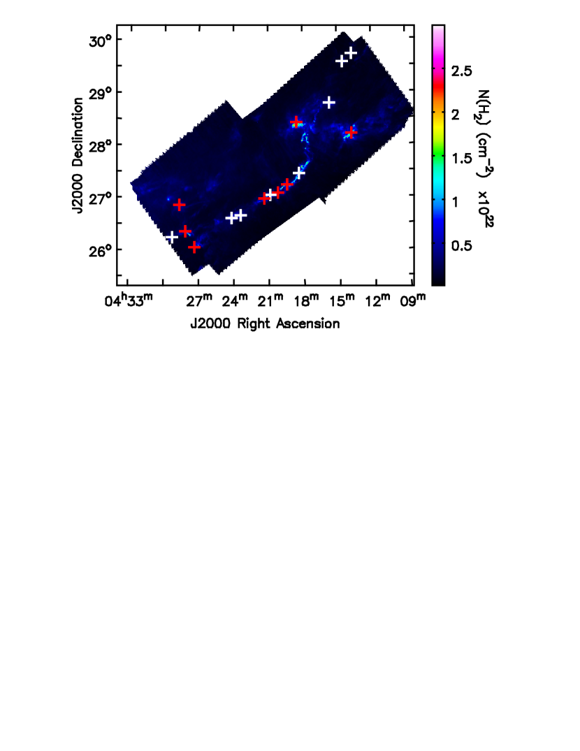
Figure 1: Spatial distribution of the observed 16 PGCCs which are marked with crosses. The red cross represents the PGCC with SCUBA-2 detection, while the white cross represents the PGCC without SCUBA-2 detection. The colour image is the Herschel H₂ column density map, which was derived from Herschel continuum data by fitting SEDs pixel-by-pixel (Marsh et al., 2016). An obvious filamentary structure in L1495 is visible.

Table 2: The coordinates of observed Planck cold clumps

Name	Glon	Glat	Ra(J2000)	Dec(J2000)	$N_{\rm VC}$	$N_{\rm core}$	$N_{\rm condensation}$
	($\arcdeg$)	($\arcdeg$)	(h m s)	(d m s)
G166.99-15.34	166.99217	-15.346058	04 13 42.01	+29 44 26.31	2	1	0
G167.23-15.32	167.23387	-15.326718	04 14 30.92	+29 35 16.09	1	1	0
G168.00-15.69	168.00291	-15.694481	04 15 40.46	+28 48 00.55	1	1	0
G168.13-16.39	168.13475	-16.393131	04 13 47.56	+28 13 22.16	2	2	3
G168.72-15.48	168.72801	-15.481486	04 18 34.58	+28 26 34.64	1	2	3
G169.43-16.17	169.43114	-16.179394	04 18 23.08	+27 28 18.97	2	2	0
G169.76-16.15	169.76073	-16.159975	04 19 25.47	+27 15 16.21	2	5	3
G170.00-16.14	170.00243	-16.140558	04 20 12.04	+27 05 52.89	2	2	2
G170.13-16.06	170.13426	-16.062908	04 20 50.61	+27 03 29.08	2	1	0
G170.26-16.02	170.2661	-16.024094	04 21 21.47	+26 59 29.26	1	2	3
G170.83-15.90	170.83739	-15.907699	04 23 24.42	+26 39 55.87	2	2	0
G170.99-15.81	170.9912	-15.810754	04 24 10.41	+26 37 16.68	1	1	0
G171.49-14.90	171.49657	-14.901693	04 28 39.71	+26 51 56.81	2	1	2
G171.80-15.32	171.80418	-15.326718	04 28 07.26	+26 21 41.65	1	3	3
G171.91-15.65	171.91405	-15.655738	04 27 20.24	+26 03 50.27	1	3	2
G172.06-15.21	172.06786	-15.210718	04 29 15.63	+26 14 52.01	1	1	0

3.1 Identification and Classification of Dense Cores

We identified dense cores within the observed PGCCs based on the column density ($N_{\rm H_{2}}$) maps derived from Herschel data by eye. We did not apply any core finder algorithm because the emission peaks in the Taurus PGCCs can be easily identified by eye. Then the identified dense cores were fitted with 2-D Gaussian to get the physical parameters (e.g., size, temperature, density). We mainly focus on the dense cores with core-averaged column densities larger than 3$\times$10²¹ cm^-2. The density threshold we used is about half of the minimum density threshold ($\sim$7$\times$10²¹ cm^-2) for core formation discovered in Herschel observations(André et al., 2014). Their peak column densities are also larger than $\sim$7$\times$10²¹ cm^-2. In total 30 most reliable dense cores with mean column densities larger than 3$\times$10²¹ cm^-2 are identified in 16 clumps from Herschel data.

As mentioned in section 1, dense cores that have no protostars are classified as starless cores. When starless cores become dense enough to be gravitationally bound, they become prestellar cores (Ward-Thompson et al., 1994). Then, the dense cores will collapse to form Class 0 and then Class I protostars.

To investigate how core properties change with evolution, we classify the dense cores into starless, prestellar, and protostellar categories. The presence of a Herschel 70 $\micron$ source is a signpost of ongoing star formation (Könyves et al., 2015). Therefore, those dense cores with 70 $\micron$ emission are protostellar. In contrast, those having no 70 $\micron$ emission are starless. As an example, Figure 2 presents the Herschel column density map (in contours) overlaid on Herschel 70 $\micron$ emission map for a representative source PGCC G171.91-15.65. The cores “H1” and “H2” in G171.91-15.65 are associated with protostars, while “H3” is starless. In this paper, we only show images for G171.91-15.65. The images for other PGCCs are shown in Appendix.

Prestellar cores are gravitationally bound starless cores and show higher density than unbound starless cores. Many factors like gravity, turbulence, magnetic field, external pressure, and even bulk motions can affect the stability of dense cores. Therefore, it is hard to tell whether or not a starless core is gravitationally bound based on present line data. The dense starless cores detected by SCUBA-2, however, having higher density than other starless cores (e.g. those without SCUBA-2 detection), should be good candidates for prestellar cores (Ward-Thompson et al., 2016). Therefore, in this paper, we classify the starless cores with SCUBA-2 detection as prestellar core candidates. In total, we identify 9 protostellar cores, 6 prestellar core candidates and 15 starless cores. The starless cores, prestellar core candidates, and protostellar cores are marked with 1, 2, or 3 in column 10 of Table 3, respectively.

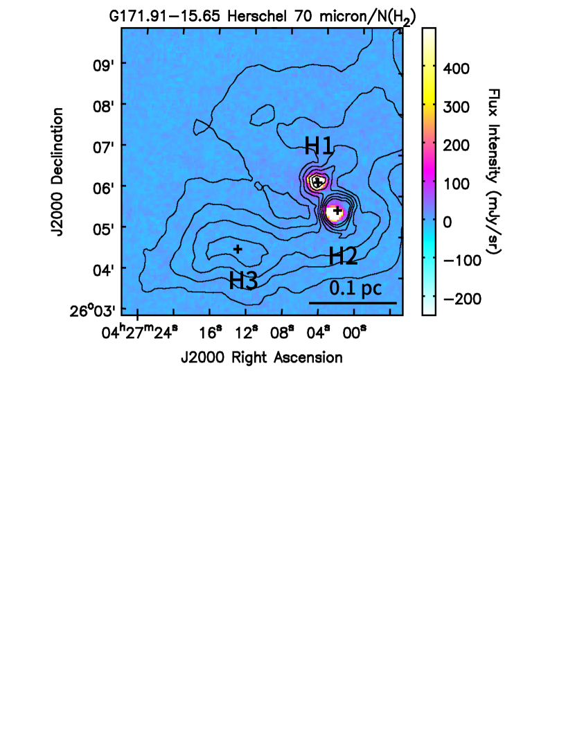
Figure 2: The Herschel column density map has overlaid on Herschel 70 $\micron$ continuum emission map for the representative source PGCC G171.91-15.65. The images for other sources are shown in Appendix. Contours represent the column density distribution from Herschel. The contour levels are from 30% to 90% of peak value, in step 10%. The Herschel 70 $\micron$ continuum are shown in colour. Protostellar cores “H1” and “H2” are associated with 70 $\micron$ sources, while starless core “H3” is not associated with any 70 $\micron$ source.

3.2 Herschel Images

The Herschel column density distributions and dust temperature maps are shown in contours and color in panel a of Figure 3, respectively. The coordinates and FWHM deconvolved major and minor axes of the dense cores (a and b) were obtained by 2-D Gaussian fits. The effective radius is R =$\sqrt{ab}D$, where D is the distance. The core-averaged $N_{\rm H_{2}}$(Herschel) and $T_{\rm d}$ of dense cores are derived within 2 FWHM (or 2R) area, and presented in Table 3. The core-averaged $N_{\rm H_{2}}$(Herschel) of the dense cores range from 3.6($\pm$1.0)$\times$10²¹ to 2.5($\pm$0.6)$\times$10²² cm^-2. The core-averaged dust temperatures of the dense cores range from 11.1($\pm$0.4) to 13.8($\pm$0.4) K. If we assume that the dense core is a sphere with a radius of $R$, the volume density of the core is roughly $n_{\rm H_{2}}=N_{\rm H_{2}}^{\rm peak}/2R$, where $N_{\rm H_{2}}^{\rm peak}$ is peak column density of dense core. The volume densities ($n_{\rm H_{2}}$) of the dense cores range from 5.7($\pm$0.9)$\times$10³ cm^-3 to 7.9($\pm$1.4)$\times$10⁴ cm^-3. The masses of the dense cores are estimated as:

$$\it{M_{\rm core}=\frac{\rm 4}{\rm 3}\pi R^{\rm 3}\cdot n_{\rm H_{2}}\cdot m_{\rm H}\cdot\mu},$$ (2)

where $\mu$ = 2.8 is the mean molecular weight (Kauffmann et al., 2008). $m_{H}$ is the mass of a H atom. The core masses $M_{\rm core}$ are presented in Table 3.

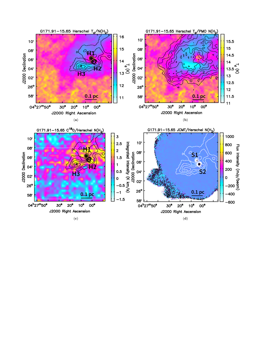
Figure 3: Panel a: The Herschel column density map have overlaid on the dust temperature map for the representative source PGCC G171.91-15.65. Contours represent the column density distributions from Herschel data. The contour levels are from 30% to 90% of peak value, in step 10%. Panel b: The PMO H₂ column density map (derived from ¹³CO data) have overlaid onto the dust temperature map for the representative source PGCC G171.91-15.65. Contours represent the column density distribution from PMO data. The contour levels are from 30% to 90% of peak value, in step 10%. The dust temperatures are shown in colour in K. Panel c: The Herschel column density map have overlaid onto the C¹⁸O integrated intensity map for the representative source PGCC G171.91-15.65. The contours represent the column density distributions from Herschel data. The contour levels are from 30% to 90% of peak value, in step 10%. The integrated intensities of C¹⁸O data are shown in colour in K km s^-1. Panel d: The Herschel column density map have overlaid on SCUBA-2 850 $\micron$ continuum emission map for the representative source PGCC G171.91-15.65. White contours represent the Herschel column density distributions. The contour levels are from 30% to 90% of peak value, in step 10%. The SCUBA-2 850 $\micron$ continuum intensities are shown in colour and black contours. The contour levels are from 10 % to 90 % of peak value, in step 20 %. The condensations detected by SCUBA-2 are marked with -S1, -S2 or -S3. Only two condensations are detected by SCUBA-2 in PGCC G171.91-15.65 and their sizes are smaller than the dense cores detected by Herschel. The same maps for other sources are shown in Appendix.

Table 3: The parameters derived from Herschel data

Name	Coordinate(J2000)	Deconvolved Size	P.A	$N_{\rm H_{2}}$(Herschel)	$N_{\rm H_{2}}^{\rm peak}$(Herschel)	$T_{d}$	R	$n_{\rm H_{2}}$	$M_{\rm core}$	Classification	Remark
	(Ra,Dec)	(”$\times$”)	($\arcdeg$)	(1022 cm-2)	(1022 cm-2)	(K)	(pc)	(104 cm-3)	(M☉)
G166.99-15.34-H1	(4:13:41.951,+29:43:43.811)	214$\times$176	-65	0.36($\pm$0.10)	0.62	13.1($\pm$0.4)	0.11	0.90($\pm$0.14)	3.6($\pm$0.6)	1
G167.23-15.32-H1	(4:14:29.120,+29:35:14.313)	233$\times$112	78	0.75($\pm$0.24)	1.19	12.5($\pm$0.4)	0.11	1.75($\pm$0.35)	6.7($\pm$1.3)	1
G168.00-15.69-H1	(4:15:35.466,+28:47:23.381)	480$\times$307	-86	0.59($\pm$0.14)	0.92	12.7($\pm$0.3)	0.26	0.57($\pm$0.09)	29.2($\pm$4.4)	1
G168.13-16.39-H1	(4:13:49.122,+28:12:31.360)	382$\times$164	-40	1.53($\pm$0.39)	2.54	11.9($\pm$0.3)	0.17	2.42($\pm$0.37)	34.6($\pm$5.3)	3	S1
G168.13-16.39-H2	(4:14:08.510,+28:09:24.391)	627$\times$164	-40	1.33($\pm$0.14)	1.64	11.6($\pm$0.2)	0.22	1.22($\pm$0.11)	36.4($\pm$3.1)	3
G168.72-15.48-H1	(4:18:33.568,+28:26:56.805)	394$\times$158	-6	1.40($\pm$0.22)	1.97	11.9($\pm$0.3)	0.17	1.89($\pm$0.21)	26.5($\pm$3.0)	1
G168.72-15.48-H2	(4:18:38.298,+28:23:22.959)	251$\times$169	-85	2.46($\pm$0.60)	4.13	13.2($\pm$1.0)	0.14	4.78($\pm$0.70)	37.8($\pm$5.5)	2	S1
G169.43-16.17-H1	(4:18:20.859,+27:28:27.755)	616$\times$152	-43	1.05($\pm$0.23)	1.49	11.9($\pm$0.3)	0.21	1.16($\pm$0.18)	30.3($\pm$4.7)	1
G169.43-16.17-H2	(4:18:36.843,+27:22:20.914)	309$\times$137	-8	0.99($\pm$0.18)	1.35	11.8($\pm$0.3)	0.14	1.57($\pm$0.21)	12.3($\pm$1.7)	1
G169.76-16.15-H1	(4:19:01.227,+27:16:50.760)	215$\times$119	-27	0.97($\pm$0.12)	1.17	11.9($\pm$0.2)	0.11	1.74($\pm$0.18)	6.5($\pm$0.7)	1
G169.76-16.15-H2	(4:19:12.104,+27:13:53.438)	232$\times$129	-37	0.95($\pm$0.09)	1.09	12.2($\pm$0.1)	0.12	1.51($\pm$0.12)	7.1($\pm$0.6)	1
G169.76-16.15-H3	(4:19:24.655,+27:15:05.860)	206$\times$124	-48	1.05($\pm$0.26)	1.70	12.1($\pm$0.3)	0.11	2.53($\pm$0.39)	9.4($\pm$1.5)	2	S3 & 21
G169.76-16.15-H4	(4:19:37.299,+27:15:19.802)	170$\times$144	-69	1.11($\pm$0.24)	1.66	11.8($\pm$0.3)	0.11	2.53($\pm$0.37)	8.8($\pm$1.3)	1	22
G169.76-16.15-H5	(4:19:42.843,+27:13:32.947)	142$\times$78	-75	1.13($\pm$0.35)	1.84	12.0($\pm$0.3)	0.072	4.17($\pm$0.79)	4.4($\pm$0.8)	3	S1 & 23
G170.00-16.14-H1	(4:19:51.580,+27:11:33.739)	108$\times$75	-35	1.24($\pm$0.30)	1.82	11.1($\pm$0.3)	0.062	4.82($\pm$0.78)	3.2($\pm$0.5)	2	S2 & 24
G170.00-16.14-H2	(4:19:58.119,+27:10:16.257)	144$\times$79	-44	1.25($\pm$0.42)	2.32	12.2($\pm$0.8)	0.065	5.82($\pm$1.05)	4.6($\pm$0.8)	3	S1 & 25
G170.13-16.06-H1	(4:20:54.832,+27:02:42.492)	400$\times$188	-89	1.16($\pm$0.26)	1.64	11.5($\pm$0.3)	0.19	1.43($\pm$0.22)	26.8($\pm$4.3)	1	30, 31 & 32
G170.26-16.02-H1	(4:21:12.207,+27:01:17.035)	101$\times$50	-51	0.99($\pm$0.17)	1.22	12.7($\pm$0.4)	0.049	4.08($\pm$0.56)	1.3($\pm$0.2)	3	S2 & 34
G170.26-16.02-H2	(4:21:21.509,+26:59:53.620)	192$\times$85	-52	1.24($\pm$0.38)	2.19	11.1($\pm$0.4)	0.087	4.08($\pm$0.71)	7.8($\pm$1.4)	2	S3 & 33
G170.83-15.90-H1	(4:23:37.832,+26:40:21.545)	204$\times$162	48	0.53($\pm$0.13)	0.70	12.2($\pm$0.3)	0.12	0.93($\pm$0.16)	5.0($\pm$0.9)	1
G170.83-15.90-H2	(4:23:29.382,+26:38:35.041)	180$\times$110	50	0.54($\pm$0.08)	0.94	12.2($\pm$0.3)	0.096	1.58($\pm$0.13)	4.0($\pm$0.4)	1
G170.99-15.81-H1	(4:24:17.134,+26:36:54.550)	669$\times$308	-75	0.82($\pm$0.18)	1.35	11.8($\pm$0.3)	0.31	0.71($\pm$0.10)	59.8($\pm$8.1)	1	35 & 36
G171.49-14.90-H1	(4:28:39.189,+26:51:43.701)	135$\times$92	-25	2.12($\pm$0.67)	3.70	11.3($\pm$0.4)	0.076	7.87($\pm$1.43)	10.0($\pm$1.8)	3	S1
G171.80-15.32-H1	(4:28:09.290,+26:20:44.816)	148$\times$97	-60	1.50($\pm$0.51)	2.52	11.1($\pm$0.4)	0.082	5.01($\pm$1.01)	7.9($\pm$1.6)	2	S1 & 39
G171.80-15.32-H2	(4:27:54.940,+26:19:17.994)	97$\times$82	70	0.89($\pm$0.15)	1.19	12.4($\pm$0.7)	0.061	3.17($\pm$0.40)	2.0($\pm$0.3)	3	S2 & 38
G171.80-15.32-H3	(4:27:48.456,+26:18:07.157)	237$\times$122	59	1.34($\pm$0.25)	1.81	11.1($\pm$0.2)	0.12	2.54($\pm$0.32)	11.3($\pm$1.6)	2	S3 & 37
G171.91-15.65-H1	(4:27:04.261,+26:06:22.493)	86$\times$48	36	0.78($\pm$0.26)	1.35	13.8($\pm$0.4)	0.044	4.99($\pm$0.94)	1.2($\pm$0.2)	3	S1
G171.91-15.65-H2	(4:27:02.366,+26:05:24.059)	90$\times$61	30	0.98($\pm$0.39)	2.07	13.3($\pm$0.6)	0.051	6.63($\pm$1.26)	2.5($\pm$0.5)	3	S2
G171.91-15.65-H3	(4:27:13.117,+26:04:30.520)	161$\times$125	-72	0.82($\pm$0.09)	0.98	12.3($\pm$0.1)	0.096	1.64($\pm$0.16)	4.2($\pm$0.4)	1
G172.06-15.21-H1	(4:29:15.723,+26:14:00.580)	215$\times$113	-72	0.87($\pm$0.26)	1.47	12.1($\pm$0.3)	0.11	2.24($\pm$0.40)	7.7($\pm$1.4)	1

3.3 SCUBA-2 Continuum Images

Panel d of Figure 3 presents the 850 $\micron$ map from SCUBA-2 overlaid on Herschel column density map. The SCUBA-2 detected condensations are marked with -S1, -S2 or -S3. The SCUBA-2 observations filtered out the large scale ($>200\arcsec$) extended emission and only picked up the dense condensations inside the cores. Some dense cores show very flatten and extended structure, and thus their emissions are mostly filtered out in SCUBA-2 observations. In total, we identified 22 condensations with signal-to-noise ratios larger than 3 from SCUBA-2 images. According to panel d of Figure 3, the SCUBA-2 detected condensations are consistently smaller than that detected by Herschel. The total integrated fluxes of these condensations were calculated from 2-D Gaussian fits. The masses were consequently obtained using Kauffmann et al. (2008):

$$M= 0.12~{}{\rm M_{\sun}}\left(e^{1.439(\lambda/\rm mm)^{-1}(\it T/\rm 10~{}K)^{-1}}-1\right)$$ (3)

$$\left(\frac{\kappa_{\nu}}{0.01\rm~{}cm^{2}g^{-1}}\right)^{-1}\left(\frac{S_{\nu}}{\rm Jy}\right)\left(\frac{D}{100\rm~{}pc}\right)^{2}\left(\frac{\lambda}{\rm mm}\right)^{3}$$

where T is temperature, adopting the Herschel dust temperature in our calculation, D is the distance to the source, $\kappa_{\nu}$=0.012 is the dust opacity at 850 $\micron$ wavelength, which is consistent with the value used in SED fit to the Herschel data in section 2.1. S_ν is the total flux density of the core region. The masses of the 22 SCUBA-2 condensations range from 0.02($\pm$0.01) M_☉ to 1.25($\pm$0.13) M_☉ and the column densities range from 4.2($\pm$0.5)$\times$10²¹ cm^-2 to 8.1($\pm$0.3)$\times$10²² cm^-2. The volume densities range from 1.5($\pm$0.2)$\times$10⁴ cm^-3 to 1.4($\pm$0.06)$\times$10⁶ cm^-3. All core parameters derived from SCUBA-2 data are presented in Table 4.

SCUBA-2 can detect the condensations denser than that detected by Herschel. The Herschel volume densities of dense cores range from 5.7($\pm$0.9)$\times$10³ to 7.9($\pm$1.4)$\times$10⁴ cm^-3. The volume densities derived from SCUBA-2 data range from 7.4($\pm$1.5)$\times$10³ to 9.1($\pm$0.6)$\times$10⁵ cm^-3. The volume density estimated from the SCUBA-2 data is larger than the value estimated from the Herschel data, indicating that the SCUBA-2 detected condensations are denser than dense cores detected by Herschel. Figure 4 presents the correlation between $M_{\rm condensation}$(SCUBA-2) and $M_{\rm core}$(Herschel). The gray area represent mass ratios which range from 0.025 to 0.125. The green squares and red diamonds represent prestellar candidates and protostellar cores, respectively. All presetllar candidates in Figure 4 are covered by gray area, but most protostellar cores show mass ratios higher than 0.125. This indicates that protostellar cores are generally more concentrated than prestellar candidates. This may indicate that as core evolve, the volume density distributions of dense cores will be more centrally concentrated.

Ward-Thompson et al. (2016) identified 25 dense condensations in L1495 cloud based on SCUBA-2 observations. According to their results, the mass of dense condensations ranges from 0.02 to 0.61 M_☉, with a mean value of 0.19. Their radii ranges from 0.02 to 0.03 pc, with a mean value of 0.03 pc. It should be noted that they have taken $\beta$ as 1.3 to derived $\kappa_{\nu}$ in their calculations. If $\beta$=2 was taken, their condensations’ masses should be doubled and are very similar to our SCUBA-2 detected condensations in PGCCs (mass ranges from 0.02 to 1.25 M_☉, with a mean value of 0.45 M_☉, radii ranges from 0.02 to 0.06 pc, with a mean value of 0.03 pc.)

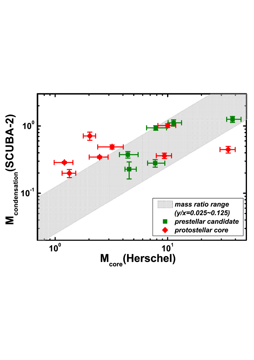
Figure 4: The correlation between $M_{\rm core}$(Herschel) and $M_{\rm condensation}$(SCUBA-2). The green squares and red diamonds represent prestellar candidates and protostellar cores, respectively. The gray area is mass ratios range (0.025$\sim$0.125). All prestellar candidates are covered by gray area, but most protostellar cores show mass ratio higher than 0.125.

Table 4: The parameters of the dense cores derived from SCUBA-2 850 $\micron$ data

Name	Coordinate(J2000)	Total flux	Peak flux density	Deconvolved size	P.A	R(SCUBA-2)	$N_{\rm H_{2}}$(SCUBA-2)	$n_{\rm H_{2}}$	$M_{\rm condensation}$	Remark
	(Ra,Dec)	(mJy)	(mJy)	(”$\times$”)	($\arcdeg$)	(10-2 pc)	(1021 cm-2)	(104 cm-3)	(M☉)
G168.13-16.39-S1	(4:13:48.350,+28:12:31.114)	1096($\pm$140)	80.40	72$\times$50	20	4.10	5.63($\pm$0.65)	2.23($\pm$0.26)	0.44($\pm$0.05)	H1
G168.13-16.39-S2	(4:13:54.792,+28:11:33.400)	66($\pm$20)	71.60	14$\times$14	0	0.95	5.39($\pm$1.14)	9.20($\pm$1.95)	0.02($\pm$0.01)
G168.72-15.48-S1	(4:18:39.688,+28:23:24.070)	4038($\pm$182)	183.43	89$\times$51	-79	4.63	12.49($\pm$1.27)	4.39($\pm$0.45)	1.25($\pm$0.13)	H2
G168.72-15.48-S2	(4:18:39.116,+28:21:56.082)	1229($\pm$139)	75.57	116$\times$37	-77	4.50	4.16($\pm$0.44)	1.50($\pm$0.16)	0.40($\pm$0.04)
G168.72-15.48-S3	(4:18:03.409,+28:22:52.354)	1424($\pm$195)	102.70	126$\times$35	84	4.55	4.74($\pm$0.59)	1.69($\pm$0.21)	0.46($\pm$0.06)
G169.76-16.15-S1	(4:19:42.596,+27:13:38.231)	1166($\pm$128)	424.45	23$\times$20	-74	1.48	34.88($\pm$3.22)	38.20($\pm$3.53)	0.40($\pm$0.03)	H5
G169.76-16.15-S2	(4:19:41.612,+27:16:08.184)	177($\pm$37)	144.54	14$\times$14	0	0.95	12.50($\pm$1.83)	21.36($\pm$3.14)	0.05($\pm$0.01)
G169.76-16.15-S3	(4:19:23.793,+27:14:54.189)	1034($\pm$125)	76.65	84$\times$37	-74	3.83	5.42($\pm$0.60)	2.29($\pm$0.25)	0.37($\pm$0.04)	H3
G170.00-16.14-S1	(4:19:58.676,+27:09:58.420)	1346$\pm$174)	396.04	26$\times$24	58	1.74	34.05($\pm$4.53)	31.69($\pm$4.22)	0.48($\pm$0.06)	H2
G170.00-16.14-S2	(4:19:51.105,+27:11:27.498)	632($\pm$110)	81.79	59$\times$41	58	3.36	4.29($\pm$0.65)	2.07($\pm$0.31)	0.23($\pm$0.03)	H1
G170.26-16.02-S1	(4:21:07.522,+27:02:31.323)	257($\pm$67)	56.54	31$\times$25	-49	1.93	5.01($\pm$1.09)	4.22($\pm$0.92)	0.09($\pm$0.02)
G170.26-16.02-S2	(4:21:11.866,+27:01:13.907)	578($\pm$81)	83.59	49$\times$21	-54	2.19	8.74($\pm$1.20)	6.47($\pm$0.88)	0.20($\pm$0.03)	H1
G170.26-16.02-S3	(4:21:21.236,+26:59:53.873)	798($\pm$96)	70.25	70$\times$25	-54	2.91	7.03($\pm$0.90)	3.92($\pm$0.50)	0.28($\pm$0.04)	H2
G171.49-14.90-S1	(4:28:39.417,+26:51:37.576)	2734($\pm$150)	249.51	60$\times$45	-13	3.56	17.00($\pm$1.08)	7.75($\pm$0.49)	1.01($\pm$0.06)	H1
G171.49-14.90-S2	(4:29:04.907,+26:49:08.135)	200($\pm$29)	170.36	14$\times$14	0	0.95	14.21($\pm$1.53)	24.28($\pm$2.61)	0.06($\pm$0.01)
G171.80-15.32-S1	(4:28:10.207,+26:20:28.341)	2667($\pm$155)	186.27	91$\times$61	63	5.07	7.73($\pm$0.60)	2.47($\pm$0.19)	0.93($\pm$0.07)	H1
G171.80-15.32-S2	(4:27:57.598,+26:19:25.435)	1735($\pm$169)	146.73	67$\times$46	64	3.81	10.43($\pm$1.46)	4.45($\pm$0.62)	0.71($\pm$0.10)	H2
G171.80-15.32-S3	(4:27:49.314,+26:18:09.353)	2871($\pm$155)	65.58	136$\times$52	63	5.76	7.15($\pm$0.78)	2.02($\pm$0.22)	1.11($\pm$0.12)	H3
G171.91-15.65-S1	(4:27:04.776,+26:06:18.335)	858($\pm$21)	88.37	14$\times$14	0	0.95	67.36($\pm$2.33)	115.07($\pm$3.97)	0.29($\pm$0.01)	H1
G171.91-15.65-S2	(4:27:02.654,+26:05:32.941)	1092($\pm$8.33)	108.65	14$\times$14	0	0.95	80.95($\pm$3.23)	138.30($\pm$5.53)	0.34($\pm$0.01)	H2

3.4 Results of PMO Molecular Lines

The ¹²CO(1-0), ¹³CO(1-0), and C¹⁸O(1-0) lines were simultaneously observed with the PMO telescope. The core-average ¹²CO(1-0), ¹³CO(1-0), and C¹⁸O(1-0) spectra of 30 Herschel dense cores are presented in Figure 5. The spectra of ¹²CO(1-0), ¹³CO(1-0), and C¹⁸O(1-0) are shown in red, green and blue, respectively. From Gaussian fitting, we obtain peak velocity, full width of half maximum (FWHM) and peak brightness temperature. Some dense cores (17 dense cores) show multiple velocity components and for these we fitted multiple Gaussian components. The fitting parameters of all dense cores are presented in Table 5. For line with multiple velocity components, the velocity component is determined to be associated with the Herschel dense core if its integrated intensity map shows similar morphology to its Herschel map.

The excitation temperature $T_{\rm ex}$ of ¹²CO is calculated following (Garden et al., 1991):

$$T_{\rm b}= \frac{T_{\rm a}^{*}}{\eta_{b}}=\frac{h\nu}{k}\left[\frac{1}{e^{(h\nu/k{T_{\rm ex}})}-1}-\frac{1}{e^{(h\nu/k{T_{\rm bg}})}-1}\right]\times$$ (4)

$$\left(1-e^{-\tau}\right)f,$$

where $T_{\rm b}$ is the brightness temperature. $T_{\rm bg}$ is the background temperature of 2.73 K. $T_{\rm a}^{*}$ is the observed antenna temperature, k is the Boltzmann constant, $\eta_{\rm b}$=0.6 is the main-beam efficiency, and $\nu$ is the frequency. Assuming that ¹²CO(1-0) is optically thick ($\tau\gg 1$) and that the filling factor f = 1, then $T_{\rm ex}$ can be obtained. The mean, maximum, minimum, median $T_{\rm ex}$ values of each dense core are presented in Table 6. The mean $T_{\rm ex}$ ranges from 8.5 K to 15.1 K, consistent with the dust temperature range.

If we assume that ¹²CO(1-0) and ¹³CO(1-0) have the same excitation temperature, the ¹³CO optical depth can be obtained. These values are also presented in Table 6. Then, the ¹³CO column density can be calculated as follows (Garden et al., 1991):

$$\it{N=\frac{{\rm 3}k}{8\pi^{\rm 2}B\mu_{\rm D}^{\rm 2}}\frac{e^{\left[hBJ(J+1)/kT_{\rm ex}\right]}}{J+1}\times\frac{T_{\rm ex}+hB/{\rm 3}k}{1-e^{(-h\nu/kT_{\rm ex})}}\int\tau_{v}dv},$$ (5)

where $B$=55101.012 MHz is the rotational constant, $\mu_{\rm D}$=0.11 debyes is permanent dipole moment for ¹³CO, and $J$ is the rotational quantum number of the lower state in the observed transition (Chackerian & Tipping, 1983). In this paper, we adopt a typical abundance ratio of [¹²CO]/[¹³CO] = 60 and [H₂]/[¹²CO] = 10⁴, considering the [¹²CO]/[¹³CO] ratio of $\sim$50 shown by Hawkins & Jura (1987) for the solar neighborhood and the ratio of $\sim$70 in the Galaxy shown by Penzias (1980). With these assumptions, the H₂ column densities are calculated and also presented in Table 6. The mean, maximum, minimum and median values of column density of each dense core are also given in columns 2 to 5, respectively. The $N_{\rm H_{2}}$ distributions, derived from PMO data, are presented in panel b of Figure 3.

The thermal velocity dispersion ($\sigma_{\rm th}$) and non-thermal velocity dispersion ($\sigma_{\rm NT}$) are calculated as:

$$\it{\sigma_{\rm NT}=\left[\sigma_{\rm{}^{\rm 13}CO}^{\rm 2}-\frac{kT_{\rm ex}}{m_{\rm{}^{\rm 13}CO}}\right]^{\rm 1/2}},$$ (6)

$$\it{\sigma_{\rm th}=\sqrt{\frac{kT_{\rm ex}}{m_{\rm H}\mu}}},$$ (7)

where $m_{\rm{}^{13}CO}$ is the mass of the ¹³CO molecule, $m_{\rm H}$ is the atomic hydrogen mass, and $\mu$ = 2.8 is the mean molecular weight of the gas (Kauffmann et al., 2008). $\sigma_{{}^{13}CO}$ is the one-dimensional velocity dispersion, obtained from second moment maps. If the velocity dispersion is isotropic, the three-dimensional velocity dispersions are calculated using:

$$\it{\sigma_{\rm 3D}=\sqrt{{\rm 3}(\sigma_{\rm th}^{\rm 2}+\sigma_{\rm NT}^{\rm 2})}}$$ (8)

The mean, maximum, minimum and median $\sigma_{\rm NT}$, $\sigma_{\rm th}$, and $\sigma_{\rm 3D}$ values of each dense core are also presented in Table 6. The mean values of $\sigma_{\rm NT}$, derived from ¹³CO, range from 0.36($\pm$0.09) km s^-1 to 0.73($\pm$0.07) km s^-1. The mean values of $\sigma_{\rm th}$ range from 0.16($\pm$0.01) to 0.21($\pm$0.01) km s^-1.

If ¹³CO is optically thick, the $\sigma_{\rm NT}$ could be overestimated. Actually, ¹³CO is optically thick in PGCCs (Wu et al., 2012). The high spectral resolution (0.16 km s^-1) in the PMO observations can also well resolve the C¹⁸O line profiles. Therefore, we also calculated $\sigma_{\rm NT}$ using C¹⁸O data, and the $\sigma_{\rm NT}$(C¹⁸O) values are presented in Table 8. The $\sigma_{\rm NT}$(C¹⁸O) values range from 0.19($\pm$0.01) km s^-1 to 0.71($\pm$0.21) km s^-1. The Mach number ($\sigma_{\rm NT}$(C¹⁸O)/$\sigma_{\rm th}$) can be calculated and listed in Table 8, where $\sigma_{\rm th}$ is the isothermal sound speed. The Mach number of dense cores range from 1($\pm$0.08) to 3.8($\pm$1.2), with a mean value of 2.1($\pm$0.8). Thus, we conclude that all the dense cores studied here have supersonic non-thermal motions.

For all of the dense cores, the Mach numbers are always greater than 1, and there is not much difference in Mach number among starless cores, prestellar core candidates, and protostellar cores. The large Mach numbers also indicate that the dense cores may be turbulence-dominated. The non-thermal velocity dispersions. however, could be also caused by bulk motions like infall or rotation.

The integrated intensity map of C¹⁸O(1-0) are shown in panel c of Figure 3. The C¹⁸O map is very noisy (the average signal-to-noise ratio of C¹⁸O mapping region is 4.1$\pm$1.2). Therefore, it is hard to derive accurate C¹⁸O column density maps. Instead, we calculate core-averaged C¹⁸O column densities from the core-averaged C¹⁸O spectra.

If we assume that C¹⁸O emission is optically thin and the excitation temperature is same as Herschel dust temperature ($T_{\rm d}$), the $N_{\rm C^{18}O}$ (column density of C¹⁸O) is calculated from (Garden et al., 1991):

$$N_{C^{18}O}=4.77\times 10^{13}\frac{(T_{\rm ex}+0.89)}{e^{(-5.27/T_{\rm ex})}}\int\frac{T_{\rm a}^{\ast}(\rm C^{18}O)}{\eta_{\rm b}}dv,$$ (9)

where $T_{\rm a}^{\ast}$ is antenna temperature, and $\eta_{\rm b}$=0.6 is main beam efficiency of PMO telescope.

We applied the non-LTE code “Radex” (Van der Tak et al., 2007) to fit C¹⁸O parameters. The input parameters for Radex are volume density, kinetic temperature, and line width. We used volume density from Herschel observations and assumed that the kinetic temperature equals to the dust temperature. The line widths were obtained from Gaussian fits to the PMO C¹⁸O(1-0) spectra. The derived column density, excitation temperature and optical depth from Radex, and the LTE column density derived from PMO data are summarized in Table 7.

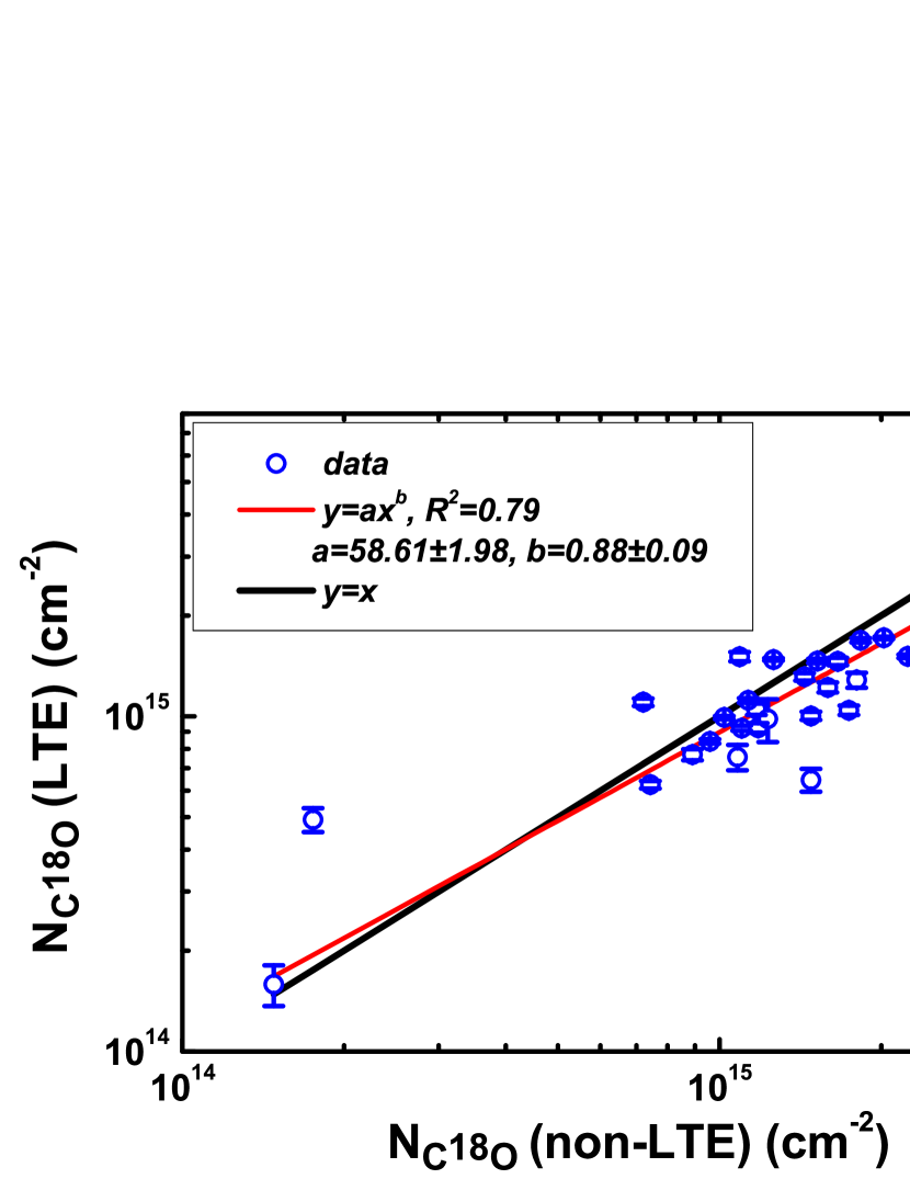
Figure 6: Relationship of the LTE C¹⁸O column density and the non-LTE C¹⁸O column density for all of the 30 dense cores in PGCCs. The red-solid line is a power-law fit. Each blue dot represents a single dense core. The black solid line is $N_{\rm C^{18}O}$(LTE) = $N_{\rm C^{18}O}$(non-LTE). The models are presented in the upper-left corner of the figure. A strong correlation can be seen very close to $N_{\rm C^{18}O}$(LTE) = $N_{\rm C^{18}O}$(non-LTE), which indicates that the LTE C¹⁸O column density estimates are reasonable.

Figure 6 shows the correlation between the LTE C¹⁸O column density and the non-LTE C¹⁸O column density. The correlation is well fitted by a power-law function, and the fitted function is close to $N_{\rm C^{18}O}$(LTE) = $N_{\rm C^{18}O}$(non-LTE), which indicates that both the calculations are reasonable.

Table 5: The parameters derived from spectra of dense cores

Name	$V_{\rm lsr}$(12)	FWHM(12)	$T_{\rm b}$(12)	$V_{\rm lsr}$(13)	FWHM(13)	$T_{\rm b}$(13)	$V_{\rm lsr}$(18)	FWHM(18)	$T_{\rm b}$(18)
	(km s-1)	(km s-1)	(K)	(km s-1)	(km s-1)	(K)	(km s-1)	(km s-1)	(K)
G166.99-15.34-H1	8.01($\pm$0.01)	0.98($\pm$0.06)	1.8($\pm$0.5)	5.65($\pm$0.04)	2.60($\pm$0.26)	0.3($\pm$0.2)
	6.38($\pm$0.02)	2.98($\pm$0.04)	4.7($\pm$0.3)	6.64($\pm$0.01)	1.80($\pm$0.04)	1.5($\pm$0.5)	6.93($\pm$0.10)	1.00($\pm$0.38)	0.2($\pm$0.1)
G167.23-15.32-H1	4.42($\pm$0.04)	1.23($\pm$0.12)	3.1($\pm$0.6)	4.23($\pm$0.24)	2.05($\pm$0.53)	0.4($\pm$0.3)
	6.92($\pm$0.04)	2.97($\pm$0.10)	5.8($\pm$0.4)	6.58($\pm$0.03)	1.54($\pm$0.08)	2.8($\pm$0.3)	6.65($\pm$0.04)	0.53($\pm$0.13)	1.0($\pm$0.3)
G168.00-15.69-H1	4.93($\pm$0.03)	1.22($\pm$0.05)	1.5($\pm$0.8)
	7.95($\pm$0.01)	1.81($\pm$0.01)	10.1($\pm$0.7)	7.83($\pm$0.01)	0.92($\pm$0.01)	6.4($\pm$0.2)	7.79($\pm$0.01)	0.55($\pm$0.02)	1.8($\pm$0.1)
G168.13-16.39-H1	6.22($\pm$0.01)	1.26($\pm$0.02)	8.3($\pm$0.7)	6.23($\pm$0.01)	0.61($\pm$0.01)	3.9($\pm$0.4)	6.60($\pm$0.01)	0.75($\pm$0.02)	2.8($\pm$0.2)
	7.46($\pm$0.01)	0.92($\pm$0.02)	7.2($\pm$0.7)	7.00($\pm$0.01)	0.90($\pm$0.01)	5.5($\pm$0.3)
G168.13-16.39-H2	3.60($\pm$0.06)	1.57($\pm$0.13)	2.0($\pm$0.6)
	6.81($\pm$0.02)	2.09($\pm$0.04)	8.6($\pm$0.5)	6.84($\pm$0.01)	1.24($\pm$0.01)	6.6($\pm$0.3)	6.84($\pm$0.02)	0.88($\pm$0.04)	2.1($\pm$0.2)
G168.72-15.48-H1	7.34($\pm$0.02)	3.04($\pm$0.04)	9.7($\pm$0.5)	7.34($\pm$0.02)	1.28($\pm$0.04)	6.5($\pm$0.5)	7.37($\pm$0.02)	0.57($\pm$0.04)	2.7($\pm$0.4)
G168.72-15.48-H2	7.40($\pm$0.01)	2.74($\pm$0.03)	10.3($\pm$0.4)	7.32($\pm$0.01)	1.27($\pm$0.02)	7.1($\pm$0.4)	7.31($\pm$0.01)	0.68($\pm$0.03)	3.9($\pm$0.3)
G169.43-16.17-H1	5.24($\pm$0.02)	1.80($\pm$0.04)	7.4($\pm$0.8)	5.35($\pm$0.02)	1.42($\pm$0.03)	5.0($\pm$0.8)	5.53($\pm$0.03)	1.30($\pm$0.07)	1.4($\pm$0.2)
	7.76($\pm$0.02)	1.92($\pm$0.05)	6.1($\pm$0.8)	6.93($\pm$0.15)	2.30($\pm$0.18)	1.1($\pm$0.6)
G169.43-16.17-H2	4.96($\pm$0.02)	1.89($\pm$0.05)	7.8($\pm$0.6)	5.37($\pm$0.01)	1.65($\pm$0.03)	5.6($\pm$0.3)	5.64($\pm$0.03)	0.98($\pm$0.09)	1.6($\pm$0.2)
	7.56($\pm$0.02)	1.63($\pm$0.05)	7.9($\pm$0.7)	7.52($\pm$0.03)	1.29($\pm$0.08)	2.0($\pm$0.3)
G169.76-16.15-H1	5.21($\pm$0.16)	1.67($\pm$0.16)	7.1($\pm$0.9)	5.52($\pm$0.01)	1.76($\pm$0.03)	5.2($\pm$0.4)	5.69($\pm$0.02)	1.28($\pm$0.06)	1.9($\pm$0.2)
	7.59($\pm$0.16)	1.75($\pm$0.16)	9.3($\pm$0.9)	7.85($\pm$0.03)	1.19($\pm$0.08)	1.8($\pm$0.4)
G169.76-16.15-H2	5.32($\pm$0.01)	1.39($\pm$0.02)	7.3($\pm$0.6)	5.42($\pm$0.01)	1.05($\pm$0.02)	4.4($\pm$0.8)	5.83($\pm$0.02)	1.15($\pm$0.05)	2.0($\pm$0.2)
	7.56($\pm$0.01)	1.94($\pm$0.03)	9.2($\pm$0.6)	6.71($\pm$0.03)	2.18($\pm$0.05)	3.4($\pm$0.6)
G169.76-16.15-H3	5.40($\pm$0.01)	1.39($\pm$0.01)	7.6($\pm$0.6)	5.40($\pm$0.01)	0.88($\pm$0.02)	4.5($\pm$0.5)	5.52($\pm$0.01)	0.59($\pm$0.02)	2.2($\pm$0.2)
	7.49($\pm$0.01)	1.61($\pm$0.01)	9.2($\pm$0.6)	6.84($\pm$0.02)	1.88($\pm$0.04)	3.7($\pm$0.3)	6.90($\pm$0.01)	0.72($\pm$0.04)	1.2($\pm$0.1)
G169.76-16.15-H4	5.48($\pm$0.01)	1.38($\pm$0.02)	7.6($\pm$0.5)	5.45($\pm$0.01)	0.67($\pm$0.02)	2.8($\pm$0.5)	5.59($\pm$0.03)	0.58($\pm$0.08)	0.6($\pm$0.2)
	7.58($\pm$0.01)	1.51($\pm$0.02)	8.3($\pm$0.5)	6.83($\pm$0.01)	1.64($\pm$0.03)	3.9($\pm$0.3)	6.88($\pm$0.01)	0.60($\pm$0.03)	1.6($\pm$0.2)
G169.76-16.15-H5	5.57($\pm$0.01)	1.28($\pm$0.03)	7.8($\pm$0.6)	5.59($\pm$0.02)	0.77($\pm$0.03)	3.8($\pm$0.5)	5.71($\pm$0.06)	0.89($\pm$0.13)	0.6($\pm$0.2)
	7.57($\pm$0.02)	1.58($\pm$0.04)	5.9($\pm$0.5)	6.73($\pm$0.02)	1.31($\pm$0.06)	3.9($\pm$0.4)	6.90($\pm$0.02)	0.51($\pm$0.05)	1.3($\pm$0.2)
G170.00-16.14-H1	5.47($\pm$0.02)	1.28($\pm$0.05)	7.6($\pm$0.7)	5.70($\pm$0.12)	1.25($\pm$0.18)	2.8($\pm$0.9)
	7.36($\pm$0.03)	1.56($\pm$0.07)	5.4($\pm$0.6)	6.78($\pm$0.08)	1.06($\pm$0.11)	3.6($\pm$0.9)	6.59($\pm$0.08)	1.11($\pm$0.13)	0.7($\pm$0.3)
G170.00-16.14-H2	5.30($\pm$0.02)	1.30($\pm$0.04)	7.5($\pm$0.6)	5.31($\pm$0.05)	0.88($\pm$0.11)	1.8($\pm$0.4)
	7.40($\pm$0.04)	2.12($\pm$0.09)	5.2($\pm$0.5)	6.64($\pm$0.03)	1.56($\pm$0.08)	4.4($\pm$0.4)	6.61($\pm$0.05)	1.11($\pm$0.10)	0.9($\pm$0.2)
G170.13-16.06-H1	5.94($\pm$0.02)	1.48($\pm$0.04)	7.2($\pm$0.5)	6.00($\pm$0.02)	0.96($\pm$0.03)	4.5($\pm$0.4)	5.97($\pm$0.06)	0.62($\pm$0.17)	0.6($\pm$0.3)
	7.38($\pm$0.02)	1.00($\pm$0.04)	4.2($\pm$0.6)	6.96($\pm$0.02)	0.91($\pm$0.03)	4.1($\pm$0.4)	6.85($\pm$0.03)	0.80($\pm$0.07)	1.4($\pm$0.3)
G170.26-16.02-H1	6.23($\pm$0.02)	2.36($\pm$0.04)	6.7($\pm$0.7)	6.36($\pm$0.01)	1.66($\pm$0.02)	5.1($\pm$0.4)	6.64($\pm$0.04)	1.41($\pm$0.09)	1.1($\pm$0.2)
G170.26-16.02-H2	5.99($\pm$0.05)	1.22($\pm$0.08)	6.7($\pm$1.2)	6.51($\pm$0.01)	1.24($\pm$0.01)	5.5($\pm$0.2)	6.56($\pm$0.01)	0.83($\pm$0.04)	1.6($\pm$0.1)
	7.17($\pm$0.06)	1.13($\pm$0.09)	4.9($\pm$1.2)
G170.83-15.90-H1	6.61($\pm$0.02)	1.46($\pm$0.04)	6.2($\pm$0.4)	6.53($\pm$0.01)	1.06($\pm$0.02)	5.3($\pm$0.3)	6.57($\pm$0.04)	1.17($\pm$0.12)	1.3($\pm$0.3)
G170.83-15.90-H2	6.67($\pm$0.02)	1.73($\pm$0.04)	6.2($\pm$0.5)	6.66($\pm$0.01)	1.18($\pm$0.02)	5.0($\pm$0.2)	6.79($\pm$0.07)	0.95($\pm$0.17)	1.1($\pm$0.3)
G170.99-15.81-H1	5.56($\pm$0.10)	1.06($\pm$0.16)	2.8($\pm$0.4)
	6.78($\pm$0.06)	1.13($\pm$0.18)	4.3($\pm$0.4)	6.50($\pm$0.01)	1.16($\pm$0.03)	4.8($\pm$0.2)	6.51($\pm$0.02)	0.64($\pm$0.05)	2.2($\pm$0.3)
	8.07($\pm$0.07)	0.71($\pm$0.17)	1.7($\pm$0.8)
G171.49-14.90-H1	5.95($\pm$0.16)	1.29($\pm$0.16)	7.0($\pm$0.6)	6.52($\pm$0.02)	0.92($\pm$0.04)	5.3($\pm$0.5)	6.55($\pm$0.02)	0.47($\pm$0.04)	2.4($\pm$0.4)
	7.49($\pm$0.16)	1.31($\pm$0.16)	8.4($\pm$0.7)	7.58($\pm$0.03)	0.85($\pm$0.05)	3.2($\pm$0.5)
G171.80-15.32-H1	6.90($\pm$0.26)	1.77($\pm$0.04)	7.4($\pm$0.5)	6.99($\pm$0.01)	0.96($\pm$0.02)	5.7($\pm$0.3)	6.96($\pm$0.06)	1.22($\pm$0.13)	0.9($\pm$0.2)
G171.80-15.32-H2	9.06($\pm$0.02)	2.17($\pm$0.05)	7.4($\pm$0.5)	7.23($\pm$0.02)	1.29($\pm$0.04)	5.2($\pm$0.3)	7.38($\pm$0.13)	1.67($\pm$0.30)	0.7($\pm$0.3)
G171.80-15.32-H3	7.04($\pm$0.02)	1.96($\pm$0.04)	6.7($\pm$0.4)	7.17($\pm$0.01)	1.01($\pm$0.02)	5.1($\pm$0.3)	7.12($\pm$0.11)	1.44($\pm$0.27)	0.5($\pm$0.3)
G171.91-15.65-H1	6.59($\pm$0.02)	2.36($\pm$0.04)	7.4($\pm$0.4)	6.61($\pm$0.01)	1.25($\pm$0.03)	6.2($\pm$0.3)	6.56($\pm$0.04)	0.90($\pm$0.09)	1.4($\pm$0.3)
G171.91-15.65-H2	6.54($\pm$0.02)	2.12($\pm$0.05)	7.3($\pm$0.4)	6.61($\pm$0.01)	1.14($\pm$0.02)	6.5($\pm$0.3)	6.64($\pm$0.03)	0.78($\pm$0.06)	1.9($\pm$0.3)
G171.91-15.65-H3	6.52($\pm$0.02)	1.97($\pm$0.05)	7.8($\pm$0.4)	6.60($\pm$0.01)	1.06($\pm$0.02)	6.1($\pm$0.3)	6.66($\pm$0.02)	0.69($\pm$0.06)	1.7($\pm$0.3)
G172.06-15.21-H1	6.59($\pm$0.01)	1.72($\pm$0.02)	9.3($\pm$0.2)	6.77($\pm$0.01)	1.01($\pm$0.02)	5.1($\pm$0.2)	6.81($\pm$0.01)	0.57($\pm$0.03)	1.8($\pm$0.2)

Note. — All parameters are derived from spectra of dense cores, which averaged over identified core’s region. For some dense cores, there are multiple velocity components, But there are some velocity components that don’t have ¹³CO and C¹⁸O emission. The spectral plot can be seen in Figure 5.

Table 6: The parameters of dense core derived from CO gas emission

Name	$N_{\rm H_{2}}$(PMO)				$T_{\rm ex}$				$\tau$ (13CO)	$\sigma_{\rm th}$				$\sigma_{\rm NT}$ (13CO)				$\sigma_{\rm 3D}$ (13CO)
	mean	max	min	median	mean	max	min	median		mean	max	min	median	mean	max	min	median	mean	max	min	median
	(1021 cm-2)				(K)					(km s-1)				(km s-1)				(km s-1)
G166.99-15.34-H1	2.1($\pm$0.2)	2.4	1.7	2.1	8.5($\pm$0.3)	9.0	7.8	8.4	0.34($\pm$0.03)	0.15($\pm$0.003)	0.16	0.14	0.15	0.56($\pm$0.11)	0.83	0.22	0.62	1.02($\pm$0.29)	1.45	0.45	1.11
G167.23-15.32-H1	3.0($\pm$0.4)	3.7	2.2	2.9	10.7($\pm$0.8)	12.5	9.2	10.8	0.48($\pm$0.07)	0.16($\pm$0.007)	0.17	0.15	0.16	0.65($\pm$0.21)	1.26	0.60	0.96	1.17($\pm$0.34)	2.20	1.07	1.69
G168.00-15.69-H1	4.8($\pm$0.3)	5.5	3.9	4.8	15.1($\pm$0.7)	16.8	13.9	14.9	0.78($\pm$0.07)	0.21($\pm$0.005)	0.23	0.21	0.21	0.48($\pm$0.06)	0.62	0.38	0.49	0.91($\pm$0.09)	1.14	0.75	0.92
G168.13-16.39-H1	3.2($\pm$0.3)	4.1	3.0	3.5	12.1($\pm$0.4)	13.4	11.3	12.0	0.58($\pm$0.04)	0.19($\pm$0.004)	0.20	0.19	0.19	0.37($\pm$0.04)	0.44	0.27	0.38	0.73($\pm$0.06)	0.83	0.58	0.73
G168.13-16.39-H2	3.5($\pm$0.3)	4.1	3.1	3.5	12.5($\pm$0.7)	14.1	11.4	12.3	1.30($\pm$0.20)	0.19($\pm$0.005)	0.21	0.19	0.19	0.36($\pm$0.06)	0.48	0.26	0.37	0.70($\pm$0.09)	0.91	0.55	0.72
G168.72-15.48-H1	6.8($\pm$0.5)	8.1	5.6	6.9	14.4($\pm$0.4)	16.6	12.3	14.3	1.03($\pm$0.07)	0.21($\pm$0.003)	0.73	0.19	0.21	0.73($\pm$0.07)	0.89	0.37	0.75	1.32($\pm$0.12)	1.59	0.73	1.35
G168.72-15.48-H2	6.8($\pm$0.6)	7.8	5.9	6.9	14.9($\pm$0.7)	16.6	13.7	14.9	0.84($\pm$0.07)	0.21($\pm$0.005)	0.22	0.20	0.21	0.67($\pm$0.09)	0.82	0.43	0.67	1.21($\pm$0.15)	1.47	0.84	1.21
G169.43-16.17-H1	6.1($\pm$0.4)	7.0	5.3	6.0	11.0($\pm$0.4)	12.1	10.1	11.0	1.07($\pm$0.10)	0.18($\pm$0.003)	0.19	0.18	0.18	0.58($\pm$0.05)	0.66	0.46	0.59	1.05($\pm$0.08)	1.19	0.85	1.07
G169.43-16.17-H2	1.8($\pm$0.3)	2.1	1.1	1.8	11.9($\pm$0.8)	13.7	10.6	11.8	1.07($\pm$0.17)	0.19($\pm$0.006)	0.19	0.18	0.19	0.40($\pm$0.16)	0.70	0.46	0.65	0.77($\pm$0.24)	1.27	1.00	1.18
G169.76-16.15-H1	5.3($\pm$0.4)	5.9	4.5	5.2	11.2($\pm$0.6)	12.7	10.1	11.0	1.09($\pm$0.15)	0.18($\pm$0.005)	0.20	0.18	0.18	0.53($\pm$0.04)	0.60	0.47	0.53	0.98($\pm$0.07)	1.09	0.87	0.97
G169.76-16.15-H2	4.8($\pm$0.2)	5.2	4.4	4.9	11.0($\pm$0.6)	12.4	10.1	10.8	0.85($\pm$0.10)	0.18($\pm$0.005)	0.19	0.18	0.18	0.47($\pm$0.04)	0.56	0.41	0.47	0.88($\pm$0.06)	1.01	0.78	0.86
G169.76-16.15-H3	3.5($\pm$0.3)	4.1	2.9	3.5	12.9($\pm$0.9)	14.4	10.6	13.0	0.48($\pm$0.06)	0.20($\pm$0.007)	0.19	0.18	0.18	0.51($\pm$0.07)	0.54	0.38	0.47	0.95($\pm$0.11)	0.99	0.74	0.87
G169.76-16.15-H4	3.2($\pm$0.2)	3.8	2.8	3.2	11.6($\pm$0.7)	12.5	10.2	11.8	0.66($\pm$0.08)	0.19($\pm$0.006)	0.20	0.18	0.19	0.49($\pm$0.11)	0.59	0.27	0.48	0.91($\pm$0.18)	1.06	0.57	0.89
G169.76-16.15-H5	2.5($\pm$0.3)	3.0	2.0	2.6	10.2($\pm$0.7)	11.2	9.4	10.3	0.81($\pm$0.13)	0.18($\pm$0.005)	0.20	0.18	0.19	0.45($\pm$0.14)	0.57	0.37	0.45	0.84($\pm$0.23)	1.05	0.72	0.85
G170.00-16.14-H1	3.7($\pm$0.3)	4.0	3.2	3.8	11.4($\pm$0.6)	12.4	10.4	11.7	0.59($\pm$0.06)	0.19($\pm$0.005)	0.20	0.18	0.19	0.52($\pm$0.18)	0.69	0.16	0.64	0.97($\pm$0.28)	1.24	0.42	1.16
G170.00-16.14-H2	3.8($\pm$0.7)	4.7	2.4	3.7	11.6($\pm$0.8)	13.8	10.7	11.4	0.76($\pm$0.11)	0.19($\pm$0.007)	0.21	0.18	0.19	0.59($\pm$0.10)	0.67	0.31	0.62	1.07($\pm$0.16)	1.20	0.62	1.12
G170.13-16.06-H1	5.0($\pm$0.4)	5.9	3.9	5.0	11.4($\pm$0.7)	12.8	10.1	11.5	0.72($\pm$0.09)	0.19($\pm$0.006)	0.20	0.18	0.19	0.55($\pm$0.04)	0.63	0.44	0.56	1.01($\pm$0.07)	1.13	0.82	1.02
G170.26-16.02-H1	3.9($\pm$0.3)	4.2	3.6	3.8	11.4($\pm$0.6)	12.3	10.6	11.4	1.01($\pm$0.12)	0.18($\pm$0.005)	0.22	0.16	0.18	0.43($\pm$0.02)	0.77	0.30	0.43	0.82($\pm$0.08)	1.38	0.60	0.82
G170.26-16.02-H2	4.2($\pm$0.1)	4.5	3.9	4.2	10.6($\pm$0.5)	11.4	9.7	10.7	1.42($\pm$0.21)	0.18($\pm$0.004)	0.19	0.17	0.18	0.46($\pm$0.05)	0.54	0.32	0.48	0.86($\pm$0.09)	0.98	0.63	0.88
G170.83-15.90-H1	1.7($\pm$0.4)	2.4	9.3	1.7	9.6($\pm$0.8)	11.4	8.5	9.5	1.81($\pm$0.65)	0.17($\pm$0.007)	0.19	0.16	0.17	0.39($\pm$0.14)	0.58	0.07	0.41	0.74($\pm$0.22)	1.05	0.31	0.76
G170.83-15.90-H2	1.3($\pm$0.4)	2.3	3.2	1.3	10.2($\pm$0.9)	12.4	8.1	10.2	1.28($\pm$0.32)	0.18($\pm$0.008)	0.19	0.16	0.18	0.37($\pm$0.11)	0.69	0.11	0.39	0.72($\pm$0.18)	1.24	0.34	0.73
G170.99-15.81-H1	3.8($\pm$0.9)	5.8	2.0	3.7	8.9($\pm$1.0)	11.6	7.1	8.8	1.89($\pm$1.01)	0.16($\pm$0.010)	0.19	0.15	0.16	0.58($\pm$0.18)	0.94	0.14	0.61	1.05($\pm$0.30)	1.65	0.38	1.09
G171.49-14.90-H1	4.5($\pm$0.5)	5.1	3.8	4.5	12.4($\pm$0.8)	14.0	11.6	12.2	0.88($\pm$0.12)	0.19($\pm$0.006)	0.20	0.18	0.18	0.51($\pm$0.08)	0.54	0.14	0.38	0.95($\pm$0.13)	0.99	0.39	0.73
G171.80-15.32-H1	3.9($\pm$0.5)	4.5	3.3	3.8	12.1($\pm$0.7)	13.6	11.0	12.0	1.05($\pm$0.14)	0.19($\pm$0.005)	0.20	0.18	0.19	0.43($\pm$0.13)	0.66	0.20	0.44	0.81($\pm$0.20)	1.18	0.48	0.83
G171.80-15.32-H2	4.5($\pm$0.3)	5.0	4.2	4.5	11.4($\pm$0.6)	12.9	10.6	11.5	1.02($\pm$0.13)	0.19($\pm$0.005)	0.20	0.18	0.19	0.65($\pm$0.06)	0.75	0.46	0.66	1.16($\pm$0.11)	1.32	0.86	1.19
G171.80-15.32-H3	3.7($\pm$0.3)	4.2	3.1	3.6	10.8($\pm$0.4)	11.6	10.3	10.7	1.14($\pm$0.10)	0.18($\pm$0.003)	0.19	0.18	0.18	0.66($\pm$0.07)	0.76	0.53	0.66	1.19($\pm$0.11)	1.36	0.97	1.18
G171.91-15.65-H1	4.8($\pm$0.3)	5.3	4.3	4.6	11.4($\pm$0.5)	12.3	10.8	11.4	1.49($\pm$0.19)	0.19($\pm$0.004)	0.19	0.18	0.19	0.42($\pm$0.09)	0.52	0.27	0.43	0.80($\pm$0.13)	0.96	0.57	0.81
G171.91-15.65-H2	4.6($\pm$0.5)	5.3	3.6	4.7	11.3($\pm$0.4)	12.1	10.9	11.3	1.64($\pm$0.19)	0.19($\pm$0.003)	0.19	0.18	0.19	0.43($\pm$0.08)	0.53	0.27	0.43	0.80($\pm$0.14)	0.97	0.13	0.80
G171.91-15.65-H3	4.4($\pm$0.2)	4.5	3.8	4.2	12.2($\pm$0.5)	13.0	11.0	12.1	1.16($\pm$0.12)	0.19($\pm$0.004)	0.20	0.18	0.19	0.36($\pm$0.09)	0.48	0.23	0.40	0.71($\pm$0.14)	0.89	0.52	0.77
G172.06-15.21-H1	3.7($\pm$0.3)	4.3	3.2	3.7	13.3($\pm$0.4)	13.9	12.4	13.2	0.71($\pm$0.05)	0.20($\pm$0.003)	0.21	0.20	0.20	0.41($\pm$0.06)	0.52	0.31	0.41	0.79($\pm$0.09)	0.97	0.64	0.79

Note. — All of this parameters are derived from the PMO observational data. Excitation temperature is calculated by ¹²CO data, $N_{H_{2}}$(PMO), $\sigma_{\rm NT}$, and $\sigma_{\rm 3D}$ are derived from ¹³CO images.

Table 7: The parameters of C¹⁸O molecules

Name	$N_{\rm C^{18}O}$(LTE)	C18O abundance(LTE)	$f_{\rm D}$	$\tau$ (C18O)	$T_{\rm ex}$(non-LTE)(C18O)	$N_{\rm C^{18}O}$(non-LTE)
	(1014 cm-2)	(10-7)			(K)	(1015 cm-2)
G166.99-15.34-H1	1.59($\pm$0.22)	0.44($\pm$0.18)	6.59($\pm$1.75)	0.02	13.99	0.15
G167.23-15.32-H1	4.92($\pm$0.40)	0.66($\pm$0.26)	4.36($\pm$1.16)	0.10	13.02	0.18
G168.00-15.69-H1	9.92($\pm$0.11)	1.69($\pm$0.42)	1.69($\pm$0.45)	0.2.	12.31	1.02
G168.13-16.39-H1	19.63($\pm$0.17)	1.28($\pm$0.34)	2.24($\pm$0.59)	0.38	12.06	2.54
G168.13-16.39-H2	17.16($\pm$0.15)	1.29($\pm$0.15)	2.22($\pm$0.59)	0.28	11.80	2.02
G168.72-15.48-H1	17.62($\pm$0.19)	1.26($\pm$0.21)	2.28($\pm$0.61)	0.37	12.08	2.24
G168.72-15.48-H2	22.32($\pm$1.55)	0.91($\pm$0.29)	3.17($\pm$0.84)	0.50	13.31	3.11
G169.43-16.17-H1	16.88($\pm$0.24)	1.61($\pm$0.38)	1.78($\pm$0.47)	0.17	12.25	1.83
G169.43-16.17-H2	14.58($\pm$0.36)	1.48($\pm$0.31)	1.95($\pm$0.52)	0.20	12.12	1.66
G169.76-16.15-H1	22.89($\pm$0.23)	2.35($\pm$0.31)	1.22($\pm$0.32)	0.24	12.19	2.69
G169.76-16.15-H2	22.05($\pm$0.10)	2.31($\pm$0.23)	1.24($\pm$0.33)	0.24	12.53	2.54
G169.76-16.15-H3	8.42($\pm$0.15)	0.80($\pm$0.21)	3.58($\pm$0.95)	0.14	12.43	0.96
G169.76-16.15-H4	9.23($\pm$0.15)	0.83($\pm$0.19)	3.46($\pm$0.92)	0.21	12.05	1.10
G169.76-16.15-H5	6.25($\pm$0.16)	0.55($\pm$0.18)	5.20($\pm$1.38)	0.16	12.20	0.74
G170.00-16.14-H1	7.56($\pm$0.29)	0.61($\pm$0.17)	4.70($\pm$1.25)	0.10	11.25	0.89
G170.00-16.14-H2	9.24($\pm$0.66)	0.74($\pm$0.30)	3.89($\pm$1.03)	0.10	12.38	1.08
G170.13-16.06-H1	10.43($\pm$0.31)	0.90($\pm$0.23)	3.18($\pm$0.84)	0.18	11.79	1.18
G170.26-16.02-H1	14.64($\pm$0.34)	1.21($\pm$0.28)	1.95($\pm$0.52)	0.14	11.57	1.74
G170.26-16.02-H2	1.22($\pm$0.22)	0.99($\pm$0.32)	2.91($\pm$0.77)	0.22	11.23	1.52
G170.83-15.90-H1	15.08($\pm$0.41)	2.87($\pm$0.76)	1.00($\pm$0.27)	0.16	12.55	1.59
G170.83-15.90-H2	10.04($\pm$0.49)	1.86($\pm$0.36)	1.54($\pm$0.41)	0.13	12.66	1.09
G170.99-15.81-H1	13.12($\pm$0.28)	1.61($\pm$0.40)	1.79($\pm$0.47)	0.30	11.72	1.48
G171.49-14.90-H1	10.21($\pm$0.34)	0.48($\pm$0.17)	5.97($\pm$1.58)	0.36	11.35	1.44
G171.80-15.32-H1	9.82($\pm$0.41)	0.66($\pm$0.25)	4.37($\pm$1.16)	0.12	11.24	1.17
G171.80-15.32-H2	10.82($\pm$1.44)	1.21($\pm$0.37)	2.36($\pm$0.63)	0.08	12.76	1.23
G171.80-15.32-H3	11.82($\pm$0.29)	0.88($\pm$0.11)	3.25($\pm$0.86)	0.06	11.37	0.72
G171.91-15.65-H1	12.82($\pm$0.51)	1.64($\pm$0.60)	1.75($\pm$0.46)	0.14	14.10	1.48
G171.91-15.65-H2	13.82($\pm$0.66)	1.42($\pm$0.68)	2.03($\pm$0.54)	0.21	13.47	1.80
G171.91-15.65-H3	14.82($\pm$0.13)	1.80($\pm$0.17)	1.60($\pm$0.42)	0.20	12.69	1.26
G172.06-15.21-H1	15.82($\pm$0.17)	1.83($\pm$0.35)	1.57($\pm$0.42)	0.22	12.39	1.13

Note. — The LTE parameters are derived from C¹⁸O spectra. The non-LTE parameters and $\tau$(C¹⁸O) are derived from the “Radex” software. The depletion factor ($f_{D}$) is calculated by $N_{\rm C^{18}O}$(LTE)

Table 8: The parameters of the dense cores

Name	$V_{\rm lsr}$(C18O)	$M_{\rm vir}$	$\alpha$	Jeans length	$\sigma_{\rm NT}$ (C18O)	Mach number
	(km s-1)	(M☉)		(pc)	(km s-1)
G166.99-15.34-H1	6.93($\pm$0.10)	23.49($\pm$17.76)	6.50($\pm$5.20)	0.375($\pm$0.011)	0.43($\pm$0.32)	2.66($\pm$2.05)
G167.23-15.32-H1	6.65($\pm$0.04)	6.48($\pm$3.06)	0.97($\pm$0.49)	0.249($\pm$0.007)	0.22($\pm$0.03)	1.22($\pm$0.20)
G168.00-15.69-H1	7.79($\pm$0.01)	16.82($\pm$1.21)	0.58($\pm$0.04)	0.440($\pm$0.010)	0.23($\pm$0.01)	1.04($\pm$0.05)
G168.13-16.39-H1	6.60($\pm$0.01)	20.20($\pm$1.02)	0.58($\pm$0.03)	0.207($\pm$0.006)	0.32($\pm$0.01)	1.65($\pm$0.07)
G168.13-16.39-H2	6.84($\pm$0.02)	35.58($\pm$3.31)	0.98($\pm$0.09)	0.244($\pm$0.004)	0.37($\pm$0.02)	1.92($\pm$0.14)
G168.72-15.48-H1	7.37($\pm$0.02)	16.66($\pm$1.22)	0.63($\pm$0.05)	0.214($\pm$0.005)	0.28($\pm$0.01)	1.37($\pm$0.05)
G168.72-15.48-H2	7.31($\pm$0.01)	9.49($\pm$1.27)	0.25($\pm$0.03)	0.164($\pm$0.013)	0.24($\pm$0.01)	1.11($\pm$0.06)
G169.43-16.17-H1	5.53($\pm$0.03)	74.28($\pm$7.64)	2.45($\pm$0.26)	0.275($\pm$0.006)	0.56($\pm$0.15)	3.04($\pm$0.89)
G169.43-16.17-H2	5.64($\pm$0.03)	28.21($\pm$5.30)	2.28($\pm$0.45)	0.231($\pm$0.005)	0.42($\pm$0.05)	2.19($\pm$0.31)
G169.76-16.15-H1	5.69($\pm$0.02)	37.45($\pm$3.46)	5.78($\pm$0.62)	0.205($\pm$0.004)	0.55($\pm$0.19)	2.96($\pm$1.10)
G169.76-16.15-H2	5.83($\pm$0.02)	32.81($\pm$2.56)	4.64($\pm$0.42)	0.222($\pm$0.002)	0.49($\pm$0.04)	2.69($\pm$0.30)
G169.76-16.15-H3	6.90($\pm$0.01)	11.85($\pm$1.15)	1.26($\pm$0.14)	0.202($\pm$0.005)	0.30($\pm$0.01)	1.53($\pm$0.11)
G169.76-16.15-H4	6.88($\pm$0.01)	7.97($\pm$0.78)	0.91($\pm$0.10)	0.189($\pm$0.005)	0.25($\pm$0.01)	1.33($\pm$0.09)
G169.76-16.15-H5	6.90($\pm$0.02)	3.86($\pm$0.73)	0.87($\pm$0.20)	0.157($\pm$0.004)	0.21($\pm$0.01)	1.19($\pm$0.10)
G170.00-16.14-H1	6.59($\pm$0.08)	16.00($\pm$3.62)	4.97($\pm$1.37)	0.128($\pm$0.004)	0.47($\pm$0.09)	2.54($\pm$0.56)
G170.00-16.14-H2	6.61($\pm$0.05)	16.68($\pm$3.01)	3.66($\pm$0.81)	0.143($\pm$0.009)	0.47($\pm$0.07)	2.51($\pm$0.46)
G170.13-16.06-H1	6.85($\pm$0.03)	25.16($\pm$4.34)	0.94($\pm$0.17)	0.240($\pm$0.007)	0.34($\pm$0.03)	1.82($\pm$0.19)
G170.26-16.02-H1	6.64($\pm$0.04)	20.28($\pm$2.53)	15.08($\pm$3.43)	0.146($\pm$0.004)	0.60($\pm$0.10)	3.28($\pm$0.63)
G170.26-16.02-H2	6.56($\pm$0.01)	12.67($\pm$1.07)	1.63($\pm$0.17)	0.153($\pm$0.006)	0.35($\pm$0.02)	1.97($\pm$0.13)
G170.83-15.90-H1	6.57($\pm$0.04)	35.56($\pm$7.05)	7.09($\pm$1.66)	0.305($\pm$0.007)	0.50($\pm$0.23)	2.92($\pm$1.48)
G170.83-15.90-H2	6.79($\pm$0.07)	18.27($\pm$6.41)	4.53($\pm$1.68)	0.267($\pm$0.006)	0.40($\pm$0.09)	2.30($\pm$0.61)
G170.99-15.81-H1	6.51($\pm$0.02)	26.87($\pm$3.84)	0.45($\pm$0.07)	0.377($\pm$0.009)	0.27($\pm$0.02)	1.66($\pm$0.20)
G171.49-14.90-H1	6.55($\pm$0.02)	3.60($\pm$0.65)	0.36($\pm$0.07)	0.111($\pm$0.004)	0.19($\pm$0.01)	1.00($\pm$0.08)
G171.80-15.32-H1	6.96($\pm$0.06)	25.72($\pm$5.42)	3.27($\pm$0.77)	0.134($\pm$0.005)	0.52($\pm$0.12)	2.72($\pm$0.72)
G171.80-15.32-H2	7.38($\pm$0.13)	35.66($\pm$12.67)	17.46($\pm$7.27)	0.167($\pm$0.010)	0.71($\pm$0.21)	3.83($\pm$1.20)
G171.80-15.32-H3	7.12($\pm$0.11)	50.51($\pm$19.20)	4.47($\pm$1.75)	0.169($\pm$0.004)	0.62($\pm$0.25)	3.40($\pm$1.42)
G171.91-15.65-H1	6.56($\pm$0.04)	7.50($\pm$1.45)	6.17($\pm$2.15)	0.169($\pm$0.005)	0.38($\pm$0.04)	2.06($\pm$0.24)
G171.91-15.65-H2	6.64($\pm$0.03)	6.40($\pm$0.96)	2.56($\pm$0.58)	0.157($\pm$0.007)	0.33($\pm$0.02)	1.76($\pm$0.13)
G171.91-15.65-H3	6.66($\pm$0.02)	9.61($\pm$1.53)	2.27($\pm$0.41)	0.218($\pm$0.002)	0.29($\pm$0.02)	1.50($\pm$0.11)
G172.06-15.21-H1	6.81($\pm$0.01)	7.30($\pm$0.79)	0.94($\pm$0.12)	0.219($\pm$0.006)	0.24($\pm$0.01)	1.18($\pm$0.05)

.

Note. — $\alpha$ is alculated by $M_{\rm vir}$/$M_{\rm core}$, and the other parameters are derived from C¹⁸O data.

Figure 5: Average spectra of 3 dense cores for the representative source PGCC G171.91-15.65. The images for other sources are shown in Appendix. For each plot, the three lines of ¹²CO, ¹³CO, and C¹⁸O are in red, green, and blue, respectively. The offsets of dense cores are presented in the upper-left corner in unit of arc-second, and they are measured relative to coordinates of PGCCs released by Planck Collaboration et al. (2016). The core names are labeled in the upper of each panel.

4 DISCUSSION

4.1 Stabilities Of Dense Cores

The gravitational stability is a critical factor to determine whether a dense core is gravitationally bound or not. Assuming a Gaussian velocity distribution and an uniform density distribution, the dense core may be supported solely by random motions. For this configuration, a virial mass can be estimated using (MacLaren, Richardon & Wolfendale, 1988):

$$\it{M_{\rm vir}={\rm 2.10}\times 10^{\rm 2}\left(\frac{R}{\rm pc}\right)\left(\frac{\Delta V}{\rm km~{}s^{-1}}\right)^{\rm 2}}\rm M_{\sun},$$ (10)

where $\Delta V$ is the FWHM of C¹⁸O spectrum, which is derived from averaged C¹⁸O spectra over the Herchel dense core, and $R$ is the radius of the Herschel dense core. The $M_{\rm vir}$ values of 30 cores range from 3.6($\pm$0.7) M_☉ to 74($\pm$7.6) M_☉ (see Table 8).

We also calculated the virial parameter $\alpha$ = $M_{\rm vir}$/$M_{\rm core}$. Kauffmann, Pillai & Goldsmith (2013) and Friesen et al. (2016) consider $\alpha$ = 2 as a lower limit for gas motions to prevent collapse, unless the dense cores are supported by significant magnetic field or confined by external presure. The virial parameter of the dense cores analyzed here ranges from 0.3($\pm$0.1) to 17.5($\pm$7.3). Fourteen dense cores have virial parameters smaller than 2 and hence are gravitationally bound and may collapse. In Figure 7, we plot $M_{\rm core}$ against $M_{\rm vir}$ and the black dashed line indicates $M_{\rm vir}$ = 2$M_{\rm core}$. We find that some protostellar cores and prestellar core candidates have virial parameters larger than 2. This apparent discrepancy might be due to:

1. Turbulence contributions: Turbulence is only dissipated in the densest regions of clouds, while the PMO observations cannot resolve such small-scale dense regions. The size of C¹⁸O core can be larger than the Herschel continuum core so that the C¹⁸O line width may include significant contributions from its turbulent surroundings. For example, Pattle et al. (2015) found that non-thermal line widths decrease substantially between the gas traced by C¹⁸O and that traced by N₂H⁺ in the dense cores of the Ophiuchus molecular cloud, indicating the dissipation of turbulence at higher densities.

2. C¹⁸O depletion: The depletion of C¹⁸O at the inner core region makes the C¹⁸O(1-0) line a poor tracer at those locations. Thus, the C¹⁸O line width is determined more by the gas outer, more turbulent regions. The presence of a central region affected by strong CO depletion could be the most important factor of uncertainty in the virial parameter (Giannetti et al., 2014).

Both of these factors can lead to an overestimation of the virial parameter. C¹⁸O lines, however, have been often used for virial analysis. For comparison, we plot the data from Onishi et al. (1996), Tachihara, Mizuno & Fukui (2000) and Zhang et al. (2015) in gray stars, orange circles and black triangles respectively in Figure 7 and Figure 8. The virial masses in those works were also calculated with C¹⁸O lines. In contrast to dense cores in other works, the cores in L1495 have similar but relatively larger virial parameters. We found that dense cores in far-away infrared dark clouds (Zhang et al., 2015; Ohashi et al., 2016; Sanhueza et al., 2017) have much smaller virial parameter than Taurus cores, suggesting that infrared dark clouds have much denser environments for star formation. A survey by Fehér et al. (2017) found 5 out of 21 PGCCs gravitationally bound based on Herschel and CO data.

As we mentioned before, the turbulence is dissipated at denser region, C¹⁸O is affected by turbulence from outer region, and it is also significantly affected by C¹⁸O depletion. Observations of this region in nitrogen-bearing tracers with comparable resolution were presented by Seo et al. (2015). A total of 12 dense cores in our samples correspond to theirs. The mean value of non-thermal velocity dispersion derived from their NH₃ and our C¹⁸O are 0.20($\pm$0.02) km s^-1 and 0.39$\pm$0.15 km s^-1, respectively. This suggests that turbulence is considerably dissipated in more centered regions. C¹⁸O in these regions were depleted, and non-thermal velocity dispersion derived from C¹⁸O are more contributed from diffused gas. Together with above comparison, C¹⁸O lines may be not good indicators of the virial parameter especially for prestellar and protostellar cores. To clarify the situation, high-resolution observations of dense gas tracers (e.g., N₂H⁺) are needed.

Kauffmann, Pillai & Goldsmith (2013) compiled a catalog containing 1325 virial estimates for entire molecular clouds ($\gg$ 1 pc scale), clump ($\sim$ 1 pc) and cores ($\ll$ 1 pc). They suggested an anti-correlation exists between mass and virial parameter:

$$\it{\alpha}=\alpha_{0}\cdot(M/\rm 10^{3}\rm~{}M_{\sun})^{{\it h_{\alpha}}},$$ (11)

with a similar slope $h_{\alpha}$, and $\alpha_{0}$ is a range of intercepts. To highlight the trend, the equation above can be rewritten as:

$$\it{\alpha}=\alpha_{\rm min}\cdot(M/M_{\rm max})^{h_{\alpha}},$$ (12)

where $\alpha_{0}$ = $\alpha_{\rm min}\cdot$($M_{\rm max}$/10³ M_☉)${}^{-h_{\alpha}}$. We fit this power law function to our 30 samples and data from Onishi et al. (1996) and Tachihara, Mizuno & Fukui (2000), the fitting results are presented in Figure 8. Data from Zhang et al. (2015) was excluded from the fitting because the number of points is small. The virial parameters from our work, Onishi et al. (1996) and Tachihara, Mizuno & Fukui (2000) follow above power law behavior, and with slope $h_{\alpha}$ of -0.74($\pm$0.08), -0.70($\pm$0.04), and -0.72($\pm$0.05), respectively. This is consistent with the range 0 $<$ - $h_{\alpha}$ $<$ 1 reported in Kauffmann, Pillai & Goldsmith (2013). Similar relationships, between virial parameters and core masses are also reported by Loren (1989) and Bertoldi & Mckee (1992). According to Figure 8, we found that these core also show similar power law behavior, indicating that these sample have similar physical properties. In Figure 7 and Figure 8, The black triangles (Zhang et al., 2015) have lowest virial parameters, and they show more star-forming activities such as outflows. This may indicate that our dense cores are at an evolutionary stages much earlier than cores reported by Zhang et al. (2015).

We also calculated the thermal Jeans length (Jeans, 1928) of dense cores and present in Table 8. We found that the radii of 30 dense cores are smaller than thermal Jeans length. Considering that all dense core have supersonic non-thermal motions, this may indicate that the non-thermal motions are capable of creating an effectively hydrostatic pressure opposing core collapse (Mac Low & Klessen, 2004).

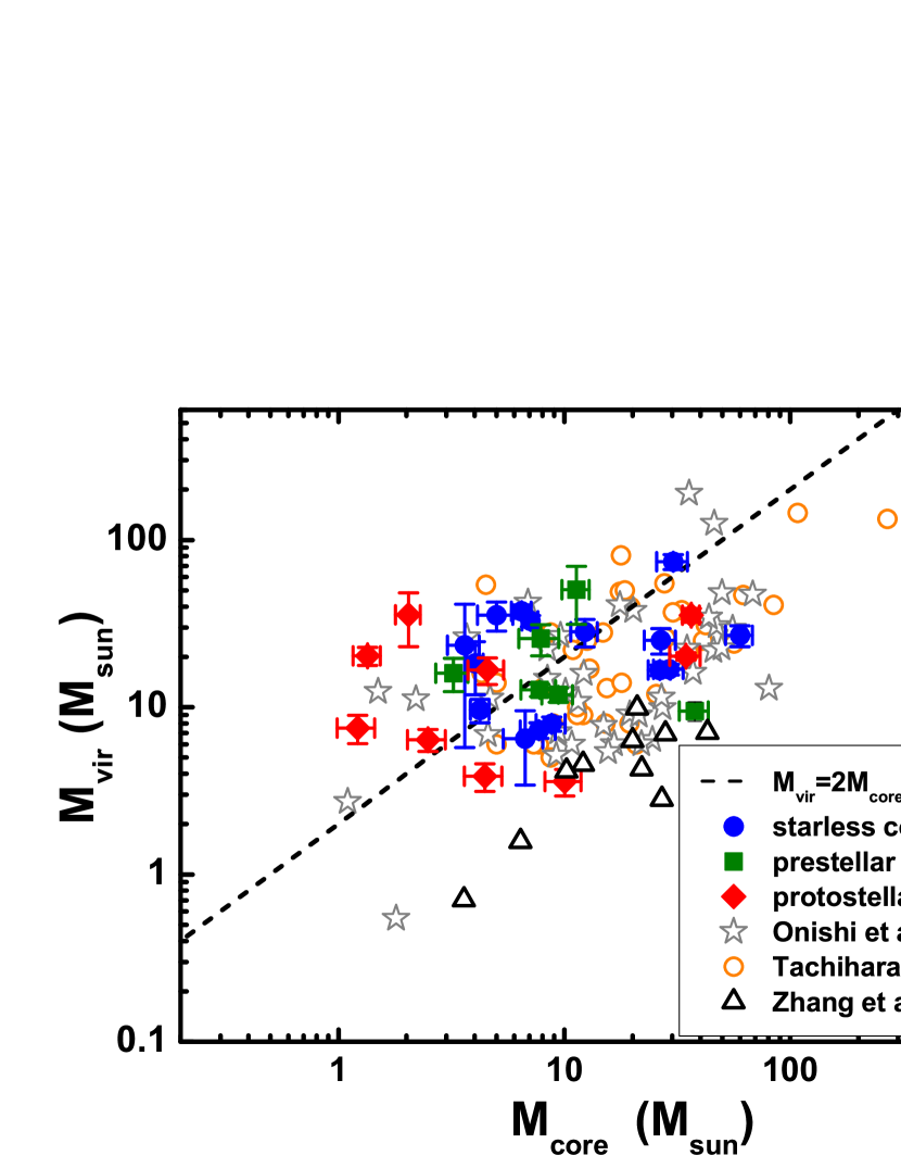
Figure 7: The relationship between $M_{\rm core}$ and $M_{\rm vir}$ of dense cores. The red diamonds, green squares and blue dots represent the protostellar cores, prestellar core candidates and starless cores, respectively. The gray stars, orange circles, and black triangles are data from Onishi et al. (1996), Tachihara, Mizuno & Fukui (2000), and Zhang et al. (2015), respectively. The black dashed line indicates $M_{\rm vir}$ = 2$M_{\rm core}$. The virial parameter $\alpha$ = 2 can be regarded as a lower limit for gas motions to prevent collapse.

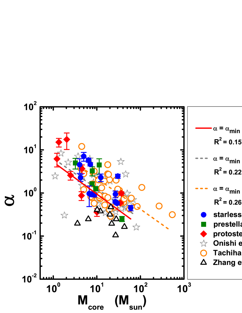
Figure 8: The relationship between $M_{\rm core}$ and $\alpha$. The red diamonds, green squares and blue dots represent the protostellar cores, prestellar core candidates and starless coress, respectively. The gray stars, orange circles, and black triangles are data from Onishi et al. (1996), Tachihara, Mizuno & Fukui (2000), and Zhang et al. (2015) respectively. The red solid, gray and orange dashed lines indicate power law fitting of $\alpha$ = $\alpha_{\rm min}\cdot$($M_{\rm core}$/$M_{\rm max}$)${}^{h_{\alpha}}$ for L1495 samples, gray stars, and orange circles, respectively.

4.2 Column Density Profile

In this section, we study the density profiles of the dense cores. We averaged the Herschel column density data in concentric elliptical bins to get a column density profile, and then fitted the Spherical Geometry Model of Dapp & Basu (2009). The underlying model resembles the Bonnor-Ebert model in that it features a flat central region leading into a power-law decline $\propto$ r^-2 in density, and a well-defined outer radius. The model can overcome the Bonnor-Ebert profile in several aspects. However, this model does not assume that the cloud is in equilibrium, and can instead make qualitative statements about its dynamical state (expansion, equilibrium, collapse) using the size of the flat region as a proxy (Dapp & Basu, 2009). Therefore, it is more suitable to study the properties of dense cores in different dynamical states.

The basic model is:

$$n(r)=\begin{cases}n_{\rm c}a^{2}/(r^{2}+a^{2})&r\leq R_{\rm t}\\ 0&r>R_{\rm t},\end{cases}$$ (13)

which is characterized by a central volume density $n_{\rm c}$ and a truncated radius $R_{\rm t}$ (In order to avoid confusion with the core radius from Gaussian fits, we use $R_{\rm t}$ to represent the truncated radius of cores derived from density profiles). The parameter a represents the size of the inner flat region of a dense core. The column density $N_{x}$ can be derived by integrating the volume density along the line of sight through the sphere. Introducing the parameter $c\equiv R_{\rm t}/a$, $N_{\rm c}=2an_{\rm c}\arctan(c)$. Hence, the model can be re-written as:

$$N_{x}=\frac{N_{\rm c}}{\sqrt{1+(x/a)^{2}}}\times\left[\arctan(\sqrt{\frac{c^{2}-(x/a)^{2}}{1+(x/a)^{2}}})/\arctan(c)\right].$$ (14)

where $N_{\rm c}$, $R_{\rm t}$, and a are free parameters. Due to their small sizes, we can not obtain average column density distributions for G170.26-16.02-H1 and G171.91-16.15-H1. Therefore, we only fit Herschel column density profiles to the other 28 cores in this section. $N_{\rm c}$, $R_{\rm t}$, a, and $n_{\rm c}$ are shown in Table 9, and statistics of these parameters are summarized in Table 10.

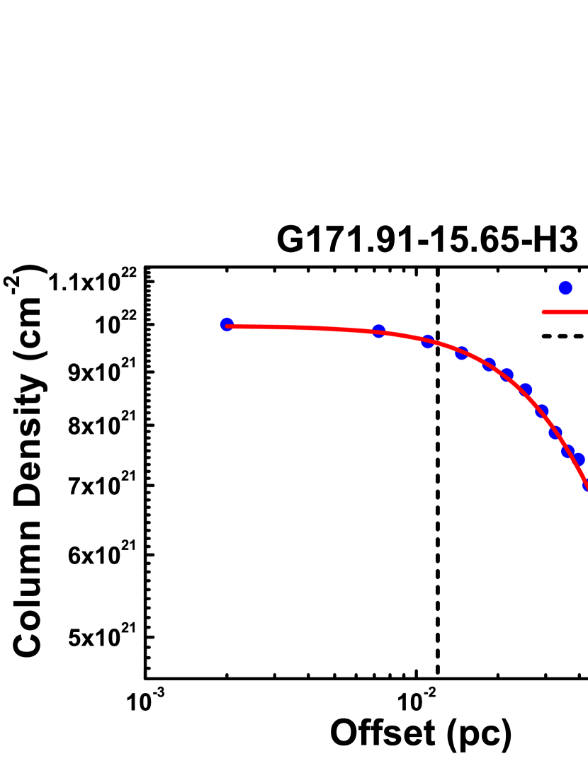
Figure 9: The column density profiles of dense core for G171.91-15.65-H3, red solid line represents the corresponding fit. Fitting results of $N_{\rm c}$, R and a are listed in Table 9. The flat central region and power-law decline can be seen in figure. Due to its small size, we can not obtain average column density distributions accurately for G170.26-16.02-H1 and G171.91-16.15-H1, and the flat region a of G171.91-15.65-H1 is smaller than beam size. Therefore, we only present the column density profile for G171.91-15.65-H3 in this section. The images for other sources are shown in Appendix.

The beam size is a critical factor that can affect the column density profile. For example, the resolution of the column density maps from Herschel data sets a lower limit for the size of the flat region a and the core truncated radius $R_{\rm t}$. To remove beam effect, we use a quadratic rule, $a_{\rm d}$ = $(a^{2}-\theta_{beam}^{2})^{1/2}$, to compute the deconvolved size of the flat region $a_{\rm d}$. A similar method was also used to calculate the deconvolved core radius $R_{\rm d}$ ($a_{\rm d}$ and $R_{\rm d}$ are listed in Table 9). Since measured flat region of G171.91-15.65-H2 is smaller than the beam size, we cannot compute its $a_{\rm d}$, and that core was also excluded from further analyses. Therefore, we present the column density profiles of G171.91-15.65-H3 in Figure 9. The profiles for other dense cores are shown in Appendix.

The upper, middle, and bottom panels of Figure 10 present the average density profiles of starless cores, prestellar core candidates, and protostellar cores, respectively. We normalized each respective core type’s column density profile before averaging. The truncated radius $R_{\rm t}$, decreases as dense cores evolve from starless to protostellar. The size of the central flat region (a) is significantly larger in the starless cores (the mean value of a is 0.48 pc for starless cores), but comparable between the prestellar candidates and protostellar cores (both the value of a for prestellar candidates and protostellar cores are 0.26 pc). This indicates that the starless cores are less peaked than prestellar core candidates or protostellar cores.

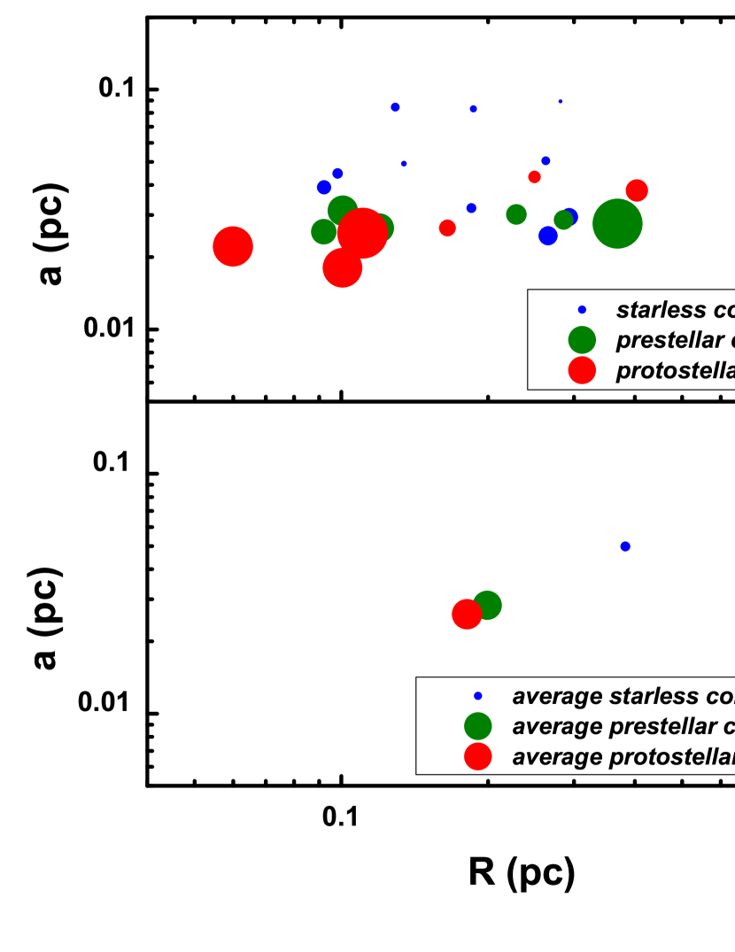
Figure 11: Top: the relationships between $R_{\rm d}$, $a_{\rm d}$, and $n_{\rm c}$ for L1495 dense cores. The x axis represents the radius $R_{\rm d}$, the y axis represents the flat region $a_{\rm d}$. The relative central volume densities $n_{\rm c}$ range from 1.3$\times$10⁴ to 1.8$\times$10⁵ cm^-3 are shown by the sizes of the data points. Bottom: The relationships between $R_{\rm d}$, $a_{\rm d}$, and $n_{\rm c}$ of averaged protostellar cores, prestellar core candidates and starless cores. In both panels, the red, green, and blue dots represent protostellar cores, prestellar core candidates, and starless cores, respectively.

Figure 11 presents $R_{\rm d}$, $a_{\rm d}$, and $n_{\rm c}$. The upper panel of Figure 11 presents the results from fits to the column density profile for each core. The red, green, and blue dots are protostellar cores, prestellar core candidates, and starless cores, respectively. The bottom panel shows the values from fits to averaged protostellar cores, prestellar core candidates, and starless cores. According to the statistics of the fitting results (see Table 10), the denser the cores are, the smaller the values of $R_{\rm d}$ and a are. In other words, the dense cores will show more steeper density structures when they evolve from starless cores to prestellar or protostellar cores.

Table 9: The parameters derived from column density profiles

Name	$N_{\rm c}$	$R_{\rm t}$	a	$n_{\rm c}$	$a_{\rm d}$	$R_{\rm d}$
	(1022 cm-2)	(pc)	(pc)	(104 cm-3)	(pc)	(pc)
G166.99-15.34-H1	0.66($\pm$0.01)	0.12($\pm$ 0.04)	0.028($\pm$0.002)	2.88($\pm$0.38)	0.025($\pm$0.002)	0.12($\pm$0.04)
G167.23-15.32-H1	1.19($\pm$0.01)	0.10($\pm$ 0.01)	0.045($\pm$0.001)	3.77($\pm$0.12)	0.043($\pm$0.001)	0.10($\pm$0.01)
G168.00-15.69-H1	0.91($\pm$0.01)	0.28($\pm$0.04)	0.089($\pm$0.005)	1.31($\pm$0.11)	0.089($\pm$0.005)	0.28($\pm$0.04)
G168.13-16.39-H1	2.68($\pm$0.01)	0.38($\pm$0.04)	0.038($\pm$0.002)	7.79($\pm$0.45)	0.036($\pm$0.002)	0.40($\pm$0.04)
G168.13-16.39-H2	1.62($\pm$0.01)	0.25($\pm$0.03)	0.043($\pm$0.006)	4.35($\pm$0.64)	0.042($\pm$0.006)	0.25($\pm$0.03)
G168.72-15.48-H1	2.10($\pm$0.01)	0.93($\pm$0.67)	0.048($\pm$0.017)	4.65($\pm$1.75)	0.047($\pm$0.017)	0.92($\pm$0.67)
G168.72-15.48-H2	4.51($\pm$0.02)	0.37($\pm$0.25)	0.028($\pm$0.001)	17.74($\pm$1.30)	0.025($\pm$0.001)	0.37($\pm$0.25)
G169.43-16.17-H1	1.51($\pm$0.01)	0.19($\pm$0.04)	0.083($\pm$0.007)	2.56($\pm$0.35)	0.082($\pm$0.007)	0.19($\pm$0.04)
G169.43-16.17-H2	1.41($\pm$0.01)	0.09($\pm$0.04)	0.039($\pm$0.017)	5.02($\pm$2.23)	0.037($\pm$0.018)	0.09($\pm$0.04)
G169.76-16.15-H1	1.20($\pm$0.01)	0.88($\pm$0.44)	0.048($\pm$0.006)	2.65($\pm$0.30)	0.047($\pm$0.005)	0.88($\pm$0.44)
G169.76-16.15-H2	1.13($\pm$0.01)	0.99($\pm$0.36)	0.053($\pm$0.005)	2.26($\pm$0.24)	0.052($\pm$0.005)	0.99($\pm$0.36)
G169.76-16.15-H3	1.80($\pm$0.01)	0.29($\pm$0.11)	0.029($\pm$0.001)	6.95($\pm$0.43)	0.026($\pm$0.001)	0.29($\pm$0.11)
G169.76-16.15-H4	1.73($\pm$0.01)	0.29($\pm$0.23)	0.029($\pm$0.002)	6.50($\pm$0.72)	0.027($\pm$0.002)	0.29($\pm$0.23)
G169.76-16.15-H5	2.18($\pm$0.03)	0.10($\pm$0.05)	0.018($\pm$0.001)	14.06($\pm$1.93)	0.014($\pm$0.002)	0.10($\pm$0.05)
G170.00-16.14-H1	1.86($\pm$0.02)	0.09($\pm$0.02)	0.026($\pm$0.002)	9.11($\pm$1.03)	0.023($\pm$0.002)	0.09($\pm$0.02)
G170.00-16.14-H2	2.36($\pm$0.03)	0.06($\pm$0.01)	0.022($\pm$0.002)	14.19($\pm$1.35)	0.019($\pm$0.002)	0.06($\pm$0.01)
G170.13-16.06-H1	1.61($\pm$0.04)	0.13($\pm$0.01)	0.085($\pm$0.012)	3.11($\pm$0.44)	0.084($\pm$0.012)	0.13($\pm$0.01)
G170.26-16.02-H2	2.30($\pm$0.01)	0.12($\pm$0.01)	0.027($\pm$0.001)	10.41($\pm$0.33)	0.024($\pm$0.001)	0.12($\pm$0.01)
G170.83-15.90-H1	0.72($\pm$0.01)	0.13($\pm$0.03)	0.049($\pm$0.004)	1.95($\pm$0.26)	0.048($\pm$0.004)	0.13($\pm$0.03)
G170.83-15.90-H2	0.96($\pm$0.01)	0.18($\pm$0.09)	0.032($\pm$0.002)	3.47($\pm$0.38)	0.030($\pm$0.002)	0.18($\pm$0.09)
G170.99-15.81-H1	1.36($\pm$0.01)	0.26($\pm$0.05)	0.050($\pm$0.002)	3.16($\pm$0.22)	0.049($\pm$0.002)	0.26($\pm$0.05)
G171.49-14.90-H1	3.79($\pm$0.03)	0.11($\pm$0.01)	0.025($\pm$0.001)	18.11($\pm$0.56)	0.022($\pm$0.001)	0.11($\pm$0.01)
G171.80-15.32-H1	2.61($\pm$0.04)	0.10($\pm$0.01)	0.031($\pm$0.002)	10.65($\pm$0.73)	0.029($\pm$0.002)	0.10($\pm$0.01)
G171.80-15.32-H2	1.37($\pm$0.01)	0.17($\pm$0.08)	0.027($\pm$0.002)	5.96($\pm$0.72)	0.024($\pm$0.002)	0.16($\pm$0.08)
G171.80-15.32-H3	1.91($\pm$0.01)	0.23($\pm$0.03)	0.030($\pm$0.001)	7.13($\pm$0.28)	0.028($\pm$0.001)	0.23($\pm$0.03)
G171.91-15.65-H2$\dagger$	2.43($\pm$0.06)	0.11($\pm$0.08)	0.010($\pm$0.001)	27.29($\pm$4.08)	…	0.11($\pm$0.08)
G171.91-15.65-H3	1.00($\pm$0.01)	0.90($\pm$0.27)	0.043($\pm$0.002)	2.46($\pm$0.13)	0.041($\pm$0.002)	0.90($\pm$0.27)
G172.06-15.21-H1	1.51($\pm$0.03)	0.27($\pm$0.09)	0.025($\pm$0.002)	6.76($\pm$0.67)	0.021($\pm$0.002)	0.27($\pm$0.08)

Note. — All of these parameters are come from fitting to column density profile. The column density profiles are derived from Herschel column density map. Due to small size of G170.26-16.02-H1 and G171.91-16.15-H1, we can not obtain their average column density distributions. Thus, we only present the parameters of 28 dense cores in this table.

Table 10: Statistics of parameters

Classification		$N_{H_{2}}$(Herschel)	$N_{H_{2}}$(PMO)	$T_{\rm d}$	$V_{\rm lsr}$	$\sigma_{\rm th}$	$\sigma_{\rm NT}$ (13CO)	$\sigma_{\rm 3D}$	$\sigma_{\rm NT}$ (C18O)	Mach number	R(Herschel)			$M_{\rm core}$	$M_{\rm vir}$	$\alpha$	Jeans length	$n_{\rm H_{2}}$	$N_{\rm C^{18}O}$	C18O abundance	$f_{\rm D}$	$a_{\rm d}$	$N_{\rm c}$	$n_{\rm c}$
		(1022 cm-2)	(1022 cm-2)	(K)	(km s-1)	(km s-1)	(km s-1)	(km s-1)	(km s-1)		(pc)			(M☉)	(M☉)		(pc)	(104 cm-3)	(1014 cm-2)	(10-7)		(pc)	(1022 cm-2)	(104 cm-3)
	Mean	1.10	0.40	12.1	6.57	0.19	0.51	0.94	0.38	2.08	0.12		Mean	13.76	21.43	3.49	0.216	2.88	12.86	1.64	1.56	0.038	1.78	6.63
all cores	Max	2.46	0.68	13.8	7.78	0.21	0.73	1.32	0.71	3.83	0.31		Max	59.83	74.28	17.46	0.440	7.87	22.89	2.87	6.59	0.089	4.51	18.11
	Min	0.36	0.13	11.1	5.37	0.16	0.36	0.70	0.19	1.00	0.044		Min	1.21	3.60	0.25	0.111	0.57	1.58	0.66	1.00	0.014	0.66	1.31
	Median	1.05	0.38	12.0	6.53	0.20	0.51	0.95	0.36	1.94	0.11		Median	7.75	17.55	2.28	0.206	2.33	12.52	1.65	2.24	0.030	1.61	5.01
	Mean	0.86	0.38	12.1	6.48	0.19	0.50	0.94	0.36	1.99	0.15		Mean	15.90	24.46	2.73	0.268	1.48	13.27	1.57	1.86	0.048	1.27	3.50
starless cores	Max	1.40	0.68	13.1	7.78	0.21	0.73	1.32	0.56	3.04	0.31		Max	59.83	74.28	7.09	0.440	2.53	22.89	2.87	6.59	0.089	2.10	6.76
	Min	0.36	0.13	11.5	5.37	0.16	0.36	0.71	0.22	1.07	0.096		Min	3.62	6.48	0.45	0.189	0.57	1.58	0.44	1.00	0.021	0.66	1.31
	Median	0.86	0.38	12.1	6.49	0.18	0.49	0.91	0.34	1.82	0.12		Median	7.73	23.49	2.27	0.240	1.57	14.58	1.61	1.74	0.047	1.20	3.11
	Mean	1.47	0.43	11.6	6.76	0.19	0.54	1.00	0.42	2.21	0.099		Mean	12.89	21.04	2.64	0.158	3.96	12.03	0.81	3.66	0.026	2.50	10.33
prestellar candidates	Max	2.46	0.68	13.2	7.19	0.21	0.67	1.21	0.62	3.41	0.14		Max	37.79	50.51	4.97	0.202	5.01	22.32	0.99	4.70	0.039	4.51	17.74
	Min	1.05	0.35	11.1	5.89	0.18	0.43	0.81	0.23	1.11	0.061		Min	3.22	9.49	0.25	0.128	2.53	0.76	0.61	2.91	0.023	1.80	6.94
	Median	1.29	0.38	11.1	6.97	0.19	0.52	0.96	0.41	2.26	0.098		Median	8.63	14.33	2.45	0.158	4.43	10.82	0.84	3.41	0.025	1.10	9.76
	Mean	1.22	0.39	12.4	6.56	0.19	0.47	0.87	0.40	2.14	0.090		Mean	10.79	16.64	5.30	0.167	4.49	12.73	1.12	3.07	0.026	2.34	10.74
protostellar cores	Max	2.12	0.47	13.8	7.10	0.19	0.64	1.16	0.71	3.83	0.22		Max	36.43	35.66	17.46	0.244	7.87	19.63	1.64	5.97	0.042	3.79	18.11
	Min	0.78	0.25	11.3	5.97	0.18	0.36	0.70	0.19	1.00	0.044		Min	1.21	3.60	0.36	0.111	1.22	0.63	0.48	1.75	0.014	1.37	4.35
	Median	1.13	0.39	12.2	6.49	0.19	0.43	0.84	0.37	1.99	0.065		Median	4.50	16.68	2.32	0.162	4.12	12.82	1.28	2.30	0.023	2.27	10.91

Note. — The statistics of main parameters for our analysis results. For all parameters, we represent the mean, maximum, minimum and median values for all cores, starless cores, prestellar candidates, and protostellar cores, respectively. However, we have not included the SCUBA-2 data in this statistic, because only a part of dense cores have been detected by SCUBA-2.

Figure 10: The average column density profile of starless cores (upper panel), prestellar core candidates (middle panel) and protostellar cores (bottom panel), respectively. Fitting results of $N_{\rm c}$, $R_{\rm t}$, and a are shown in each panel.

4.3 CO Depletion

Gaseous CO molecules can freeze out onto grain surfaces in cold and dense regions, and the CO molecules can return to the gas phase as temperature rises due to heating from protostars (Bergin & Langer, 1997; Charnley, 1997; Zhang et al., 2017).

Since C¹⁸O emission is generally optically thin, it is a more reliable tracer for CO depletion than ¹²CO or ¹³CO. We calculate the core-averaged C¹⁸O abundance of each dense core as follows:

$$X=\frac{N_{\rm C^{18}O}}{N_{\rm H_{2}}(Herschel)},$$ (15)

where $N_{\rm H_{2}}$ is the core’s Herschel-derived column density of H₂ (listed in Table 3), and $N_{\rm C^{18}O}$ is the C¹⁸O column density. It should be noted that the G166.99-15.34-H1 and G167.23-15.32-H1 are located outside of the densest parts of the filament, and with exceptionally low C¹⁸O abundances. The low C¹⁸O abundance in these two cores may be because that they are less shielded from interstellar UV radiation and the CO molecules inside them are more easily dissociated. Thus, C¹⁸O abundance of these two dense cores are very low, and they were excluded from fitting. In Figure 12, the red diamonds, green squares and blue dots represent the protostellar cores, prestellar core candidates and starless cores, respectively. C¹⁸O abundance is clearly anti-correlated with the column density, also indicating that the CO depletion becomes more prevalent in denser cores.

In this work, we simply define a relative CO depletion factor ($f_{\rm D}$) of dense cores as follows:

$${f_{\rm D}=\frac{X_{\rm max}}{X_{\rm core}}},$$ (16)

where $X_{\rm max}$ is the maximum C¹⁸O abundance in all the L1495 dense cores, and $X_{\rm core}$ is the C¹⁸O abundance of dense core. The CO depletion factors ($f_{\rm D}$) range from 1 to 6.6($\pm$1.8), and for each core these parameters are listed in Table 7. Please note that the CO depletion factors derived here should be treated as lower limits because we used core-averaged values. The CO depletion could be even more severe toward the core center.

Figure 13 presents $f_{\rm D}$ and the central volume densities ($n_{\rm c}$) of the L1495 dense cores. There is a clear positive correlation between $f_{\rm D}$ and $n_{\rm c}$, indicating that CO depletion is more significant in denser cores. The starless cores are located at bottom-left in Figure 13 and thus these cores have smallest CO depletion factors. CO depletion in prestellar candidates and protostellar cores is more significant than starless cores. The mean depletion factors of starless cores, prestellar core candidates, and protostellar cores are 1.9($\pm$0.7), 3.7($\pm$0.7), and 3.1($\pm$1.5), respectively. The prestellar candidates and protostellar cores are mixed with each other in the Figure 12 and Figure 13, indicating that the protostellar cores in L1495 are still at the earliest phases of star formation and thus have as a high degree of CO depletion as prestellar core candidates.

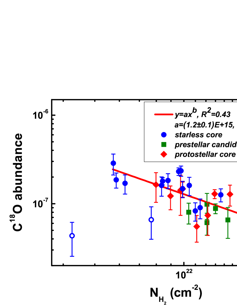
Figure 12: Correlation of C¹⁸O abundance and Herschel $N_{\rm H_{2}}$. The red line is a power-law fit. The red diamonds, green squares and blue dots represent the protostellar cores, prestellar core candidates and starless coress, respectively. The blue circles represent G166.99-15.34-H1 and G167.23-15.32-H1, they are located outside of the densest parts of the filament, Thus, we excluded them from fitting. The function and coefficients of models are presented in upper-right corner of panel. A potential anti-correlation are found in the figure.

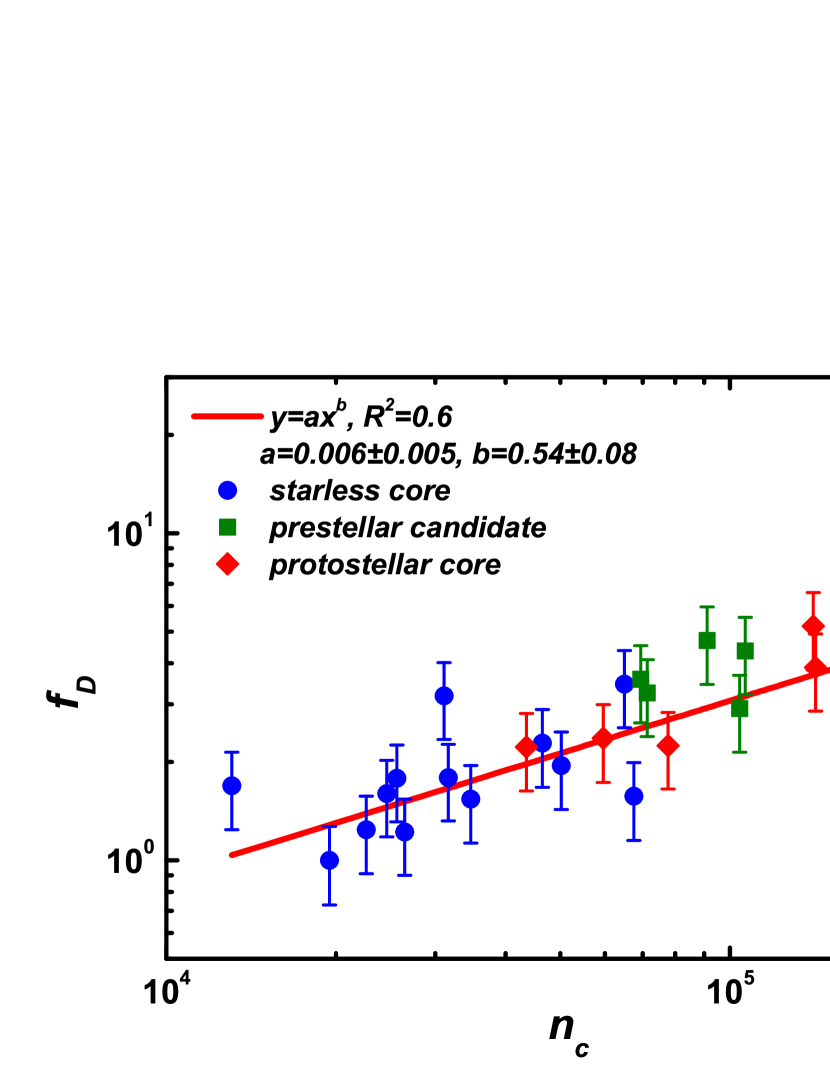
Figure 13: Correlation of relative depletion factors ($f_{\rm D}$) and the central volume densities $n_{\rm c}$ (Herschel). The red line is a power-law fit, blue dots, green squares and red diamonds represent starless cores, prestellar core candidates and protostellar cores, respectively.

5 SUMMARY

To understand better the properties of PGCCs and dense cores in L1495 cloud, we have studied 16 dense clumps in the L1495 cloud with data from Herschel, JCMT/SCUBA-2, and the PMO 13.7 m telescope. The main findings of this work are as follows:

1. In the L1495 region of Taurus, we identified 30 dense cores in 16 PGCCs. The majority of Planck clumps have Herschel cores, often multiple, but only a subset of the Herschel cores have corresponding SCUBA-2 condensations. Based on SCUBA-2 and Herschel 70 $\micron$ data, we have classified these 30 dense cores into three types: 15 are starless cores (i.e., with neither SCUBA-2 nor Herschel 70 $\micron$ emission), 6 are prestellar core candidates (i.e., with SCUBA-2 emission but without Herschel 70 $\micron$ emission) and 9 are protostellar cores (i.e., with Herschel 70 $\micron$ emission). Our findings suggest that not all PGCCs contain prestellar objects. In general, however, the dense cores in PGCCs are usually at their earliest evolutionary stages.

2. Based on Herschel data, the mean volume densities of the starless cores, prestellar core candidates and protostellar cores are 1.0($\pm$0.4)$\times 10^{4}$ cm^-3 cm^-3, 2.5($\pm$0.6)$\times 10^{4}$ cm^-3, and 2.7($\pm$1.0)$\times 10^{4}$, respectively. The mean dust temperatures of the starless cores, prestellar core candidates and protostellar cores are 12.1($\pm$0.4) K, 11.6($\pm$0.8) K, and 12.4($\pm$0.7) K, respectively. On average, prestellar core candidates have slightly lower dust temperature and higher density than starless cores. The 9 protostellar cores appear to be still at the earliest protostellar evolutionary phases and the newly formed protostar have not significantly heated their envelopes.

3. Non-thermal and thermal velocity dispersions have been derived from the PMO data. In all 30 dense cores, the Mach numbers are all larger than 1, with an average value of 2.1($\pm$0.8). Hence the turbulence in the L1495 dense cores is supersonic, and all 30 dense cores may be turbulence-dominated.

4. The virial masses ($M_{\rm vir}$) derived from the C¹⁸O data range from 3.6($\pm$0.7) M_☉ to 74.3($\pm$7.6) M_☉. The virial parameters ($\alpha$) range from 0.3($\pm$0.1) to 17.5($\pm$7.3). Fourteen dense cores have virial parameters smaller than 2, and 18 dense cores have virial parameters larger than 2. The virial parameter and core mass follow the power law trend, $\alpha$ = $\alpha_{\rm min}\cdot$($M_{\rm core}$/$M_{\rm max}$)${}^{h_{\alpha}}$, with $h_{\alpha}$ = -0.74($\pm$0.08).

5. The column density profiles of 28 dense cores have been derived from Herschel data. The central volume density ($n_{\rm c}$), the size of flat region (a) and the truncated radius ($R_{\rm t}$) were obtained by fitting a column density profile. We found that the values of flat region size and truncated radius decrease as $n_{\rm c}$ increases. This indicates that dense cores shrink as they evolve from starless cores to protostellar cores (Ward-Thompson et al., 1994).

6. The C¹⁸O abundances are used to investigate the CO depletion degree in the three types of dense cores. The mean C¹⁸O abundances of protostellar cores, prestellar core candidates, and starless cores are 1.12($\pm$0.48)$\times 10^{-7}$, 8.07($\pm$1.34)$\times 10^{-8}$ and 1.57($\pm$0.65)$\times 10^{-7}$, respectively. This variation means that CO depletion in prestellar core candidates is most significant. The core-averaged CO depletion factors ($f_{\rm D}$) range from 1 to 6.6($\pm$1.8). Our results support the idea that the C¹⁸O abundance can be used as an evolutionary tracer for molecular cloud cores, as suggested by Caselli et al. (1999); Di Francesco et al. (2007); Liu, Wu & Zhang (2013).

6 ACKNOWLEDGEMENT

S.-L. Qin is supported by the National Key R&D Program of China (NO. 2017YFA0402701), by the Joint Research Fund in Astronomy (U1631237) under cooperative agreement between the National Natural Science Foundation of China (NSFC) and Chinese Academy of Sciences (CAS), by the Top Talents Program of Yunnan Province (2015HA030). Tie Liu is supported by KASI fellowship and EACOA fellowship. Ke Wang is supported by grant WA3628-1/1 of the German Research Foundation (DFG) through the priority program 1573 (“Physics of the Interstellar Medium”). Chang Won Lee was supported by Basic Science Research Program through the National Research Foundation of Korea (NRF) funded by the Ministry of Education, Science and Technology (NRF-2016R1A2B4012593) This research was partly supported by the OTKA grant NN-111016. We thank Michel Fich, Mika Juvela, Jan Wouterloot, Archana Soam, M. R. Cunningham, Chang Won Lee, Paul F. Goldsmith, A. Rivera-Ingraham, Jinghua Yuan, Pak Shing Li, Johanna Malinen, George J. Bendo, Hong-Li Liu, Miju Kang, Neal J. Evans II, Patricio Sanhueza, Edith Falgarone, Glenn J. White, Izaskun Jimenez-Serra, You-Hua Chu, Yao-Lun Yang, JinHua He, and Hauyu Baobab Liu for helpful discussions and comments. The James Clerk Maxwell Telescope is operated by the East Asian Observatory on behalf of The National Astronomical Observatory of Japan, Academia Sinica Institute of Astronomy and Astrophysics, the Korea Astronomy and Space Science Institute, the National Astronomical Observatories of China and the Chinese Academy of Sciences (Grant No. XDB09000000), with additional funding support from the Science and Technology Facilities Council of the United Kingdom and participating universities in the United Kingdom and Canada. Additional funds for the construction of SCUBA-2 were provided by the Canada Foundation for Innovation. This research has made use of data from the Herschel Gould Belt survey (HGBS) project (http://gouldbelt-herschel.cea.fr). The HGBS is a Herschel Key Programme jointly carried out by SPIRE Specialist Astronomy Group 3 (SAG 3), scientists of several institutes in the PACS Consortium (CEA Saclay, INAF-IFSI Rome and INAF-Arcetri, KU Leuven, MPIA Heidelberg), and scientists of the Herschel Science Center (HSC).

References

- André et al. (2010) André, P., et al. 2010, A&A, 518, L102
- André et al. (2014) André, P., Di Francesco, J., Ward-Thompson, D., et al. 2014, accepted in Protostars and Planets VI University of Arizona Press, arXiv:1312.6232
- Bergin & Langer (1997) Bergin, E. A., & Langer, W. D. 1997, ApJ, 486, 316
- Bertoldi & Mckee (1992) Bertoldi, F., Mckee, C. F. 1992, ApJ, 395, 140
- Bintley et al. (2014) Bintley, D., Holland, W. S., MacIntosh, M. J., et al. 2014, SPIE, 9153E, 03B
- Buckle et al. (2015) Buckle, J. V., Drabek-Maunder, E., Greaves, J., et al. 2015, MNRAS, 449, 2472
- Caselli et al. (1999) Caselli, P., Walmsley, C. M., Tafalla, M., Dore, L., & Myers, P. C. 1999, ApJL, 523, L165
- Caselli (2011) Caselli, P. 2011, IAUS, 280, 19
- Chackerian & Tipping (1983) Chackerian, C, and Tipping, R. H. 1983, J. Molec. Spectrosc., 99,431
- Chapin et al. (2013) Chapin, E., Gibb, A. G., Jenness, T., et al. 2013, StaUN, 258, C
- Charnley (1997) Charnley, S. B. 1997, MNRAS, 291, 455
- Currie et al. (2014) Currie, M. J., Berry, D. S., Jenness, T., et al. 2014, ASPC, 485, 391
- Dapp & Basu (2009) Dapp, W. B., Basu, Shantanu. 2009, MNRAS, 395, 1092D
- Dempsey et al. (2013) Dempsey, J. T., Friberg, P., Jenness, T., et al. 2013, MNRAS, 430, 2534D
- Di Francesco et al. (2007) Di Francesco, J., Evans, II, N. J., Caselli, P., et al. 2007, Protostars and Planets V, 17
- Elias (1987) Elias, J. H. 1987, ApJ, 224, 857
- Fehér et al. (2017) Fehér, O., Juvela, M., Lunttila, T., Montillaud, J., Ristorcelli, I., Zahorecz, S., Tóth, L. V. A&A, 2017, 606, A102
- Friesen et al. (2016) Friesen, R. K., Bourke, T. L., Di Francesco, J., Gutermuth, R., & Myers, P. C. 2016, ApJ, 833, 204
- Garden et al. (1991) Garden, R. P., Hayashi, M., Hasegawa, T., Gatley, I., & Kaifu, N. 1991, ApJ, 374, 540
- Giannetti et al. (2014) Giannetti, A., Wyrowski, F., Csengeri, T., Fontani, F., Walmsley, C. M., et al. 2014, A&A, 570, A65
- Hacar et al. (2013) Hacar, A., Tafalla, M., Kauffmann, J., & Kovács, A. 2013, A&A, 554, A55
- Hawkins & Jura (1987) Hawkins, I., & Jura, M. 1987, ApJ, 317, 926
- Hildebrand (1983) Hildebrand, R. H. 1983, QJRAS, 24, 267
- Holland et al. (2013) Holland, W. S., Bintley, D., Chapin, E. L., et al. 2013, MNRAS, 430, 2513
- Jeans (1928) Jeans, J. H. 1928, Astronomy and Cosmogony (Cambridge University Press)
- Jrgensen, Schöier & van Dishoeck (2002) Jrgensen, J. K., Schöier, F. L., & van Dishoeck, E. F. 2002, A&A, 389, 908J
- Juvela et al. (2017) Juvela, M., He, J., Pattle, K., et al. 2017, A&A in press, arXiv:1711.09425
- Kauffmann et al. (2008) Kauffmann, J., Bertoldi, F., Bourke, T. L., Evens, II, N. J., & Lee, C. W. 2008, A&A, 487, 993