Extensive numerical study and circuitry implementation of the Watt governor model

Abstract

In this work we carry out extensive numerical study of a Watt-centrifugal-governor system model, and we also implement an electronic circuit by analog computation to experimentally solve the model. Our numerical results show the existence of self-organized stable periodic structures (SPSs) on parameter-space of the largest Lyapunov exponent and isospikes of time series of the Watt governor system model. A peculiar hierarchical organization and period-adding bifurcation cascade of the SPSs are observed, and this self-organized cascade accumulates on a periodic boundary. It is also shown that the periods of these structures organize themselves obeying the solutions of Diophantine equations. In addition, an experimental setup is implemented by a circuitry analogy of mechanical systems using analog computing technique to characterize the robustness of our numerical results. After applying an active control of chaos in the experiment, the effect of intrinsic experimental noise was minimized such that, the experimental results are in astonishing well agreement with our numerical findings. We can also mention as another remarkable result, the application of analog computing technique to perform an experimental circuitry analysis in real mechanical problems.

1 Introduction

The steam engine played an important role in the Industrial Revolution Hills [1989] (see also references therein) at the end of the $18^{th}$ century in Great Britain and it can be considered the starting point for the automatic control theory MacFarlane [1979]. In a tentative to automatically control the steam flux into the engine from the boiler, James Watt invented a centrifugal governor system Maxwell [1868], here called by Watt governor system (WGS). Figure 1 illustrates the mechanical WGS connected to a valve that regulates the steam flux to the engine. In this case, as the angular velocity of the Watt governor increases, the kinetic energy of the balls increases. This allows the two masses on lever arms move vertically outwards and upwards. If this motion goes far enough, a security mechanism is initialized and it goes to reduce the rate of working-fluid entering to the engine reducing its velocity, preventing the over-velocity.

The WGS is often used in the nonlinear sciences as an example of a dynamical system. Indeed, due to the rich variety of complex behaviors and historical importance the dynamics of WGS is studied here through of two different ways, as follows: (i) a numerical analysis, by solving the equations of motion with both Runge-Kutta and numerical continuation methods and, (ii) an experimental study, using a circuitry setup. These two ways to study the dynamics of WGS are self-complementary as shown at next. In the first one, a characterization of dynamics of WGS by numerical simulations can be performed by integration of the equations of motion while, in the second an analog computation technique can be used to construct a circuit setup which works, based on the equations of motion, in order to reproduce the dynamics of the original mechanical system. A real experiment with a mechanical setup using sensors coupled to WGS can also be achieved, although, it is not the goal here. However, the control parameters in the set of differential equations used to model the dynamics of WGS can also be seen as sensors for measurements of dynamical parameters in the real mechanical experiment. Before applying a detailed discussion on numerical and experimental results, it is important to introduce an appropriated theoretical model for WGS, used in our investigations.

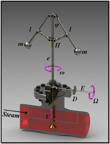
Figure 1: Schematic illustration of mechanical Watt governor system coupled to a steam pipe.

Applying the Newton’s Second Law to translational and rotational motion of the mechanical Watt governor (shown in Fig. 1), we obtain the following set of coupled differential equations

$$\left\{\begin{array}[]{ll}\dot{\varphi}=\dfrac{d\varphi}{d\tau}=\psi,\\ \\ \dot{\psi}=\dfrac{d\psi}{d\tau}=c^{2}\Omega^{2}\sin\varphi\cos\varphi-\dfrac{g}{l}\sin\varphi-\dfrac{b}{m}\psi,\\ \\ \dot{\Omega}=\dfrac{d\Omega}{d\tau}=\dfrac{1}{I}(\mu\cos\varphi-F),\end{array}\right.$$ (6)

where $\varphi\in\left(0,\frac{\pi}{2}\right)$ is the angle of deviation of the arms of the governor from its vertical axis $e$, $\Omega\in[0,\infty)$ is the angular velocity of the rotation of the flywheel $D$, $\omega$ is the angular velocity of $e$, $l$ is the length of the arms, $m$ is the mass of each ball, $H$ is a sleeve which supports the arms and slides along $e$, $T$ is a set of transmission gears, $V$ is the valve that determines the supply of steam to the engine, $\tau$ is the time, $\psi=d\varphi/d\tau$, $g$ is the standard acceleration of gravity. The angular velocity of $e$ is related to the angular velocity of the rotation of the flywheel $D$ by $\omega=c\Omega$, where $c$ is the positive constant transmission ratio. $b$ is a positive constant of the frictional force of the system, $I$ is the moment of inertia of the flywheel, $F$ is an equivalent torque of the load and $\mu$ is a positive proportionality constant. The parameters $b,c$ and $\mu$ only assume positive values to preserve the physical meaning of Eqs. (6). For a derivation of Eqs. (6), the reader is referred to Pontryagin Pontryagin [1962].

Based on Ref. Sotomayor et al. [2007], we rewrite the set of Eqs. (6) in normalized and dimensionless form as follows

$$\left\{\begin{array}[]{ll}\dot{x}=\dfrac{dx}{dt}=y,\\ \\ \dot{y}=\dfrac{dy}{dt}=z^{2}\sin x\cos x-\sin x-\varepsilon y,\\ \\ \dot{z}=\dfrac{dz}{dt}=\alpha(\cos x-\beta),\end{array}\right.$$ (12)

where

$$x=\varphi,\qquad y=\sqrt{\frac{l}{g}}\psi,\qquad z=\sqrt{\frac{l}{g}}\Omega,\qquad\tau=\sqrt{\frac{l}{g}}t,$$

and

$$\varepsilon=\frac{b}{m}\sqrt{\frac{l}{g}},\qquad\alpha=\frac{cl\mu}{gI},\qquad\beta=\frac{F}{\mu},$$

for $\varepsilon>0$, $\alpha>0$ and, $0<\beta<1$. As presented in the next section, those three parameters are varied in pairs to perform a characterization of dynamics of WGS. For example, when $\epsilon$ and $\alpha$ are varied, keeping $\beta$ fixed, it means that, in a possible mechanical experiment of Fig. 1 (not realized in present work), the length $l$ of the arms and the mass $m$ of each ball has been varied simultaneously. As a consequence, the parameters $\epsilon$, $\alpha$ and $\beta$ only assume positive values to preserve their physical meanings. The same analysis can be extended to other parameter pairs combination (as shown bellow). Numerical and experimental result sections show that, even tiny changes in one or two of those parameter values are enough to drastically change the dynamics of mechanical WGS, i.e., the analysis about how their dynamical behaviors changes when those three parameters are varied in pairs endorses the importance of the present study. Therefore, the system (12) is a three-parameter nonlinear dynamical system and extensive analyzes of stability and Hopf bifurcation in that system have been reported in Ref. Sotomayor et al. [2007] (see also references therein). Analytical and numerical studies in a hexagonal governor system can also be found in Ref. Zhang et al. [2010].

Once that system (12) is an autonomous three-dimensional continuous system, chaotic dynamics can arise Strogatz [2001] and a recent interest is on the description of its dynamics in parameter-planes simultaneously varying two control parameters Celestino et al. [2011, 2014]; Gallas [2015]; Meucci et al. [2016]; de Sousa et al. [2016]; da Costa et al. [2016]; Gallas [2016]. To construct those parameter-planes, it is usually used the Largest Lyapunov exponent (Lyapunov diagram) Gallas [2015]; Meucci et al. [2016]; de Sousa et al. [2016]; da Costa et al. [2016]; Gallas [2016]; Rech [2016] or the number of spikes in one period of the orbits (isospikes diagram) Gallas [2016]; Hoff et al. [2013] (both measures are properly defined at next). Those measures are identified by color intensities on parameter-planes. Regardless of the used measures, the two-parameter behavior of a large class of nonlinear systems usually presents a complex bifurcation scenario and generic Stable Periodic Structures (SPSs) Celestino et al. [2014] (see also references therein), namely shrimps-shaped domains, embedded in chaotic regions on the parameter-space. In some systems these structures organize themselves with specific bifurcation cascades, for example, period-adding cascades, and along preferred directions on the parameter-space Gallas [2015]; de Sousa et al. [2016]; Gallas [2016].

In this work, we report the existence of such SPSs organizing themselves along specific directions on the Lyapunov and the isospike diagrams of the WGS model (12) Sotomayor et al. [2007], using two invariant measures of the system namely, the Largest Lyapunov Exponent (LLE) and the number of spikes $q$ in one period of the time-series of the attractors, respectively. The results presented here, corroborate the generic nature of those SPSs, independently of the systems’ nonlinearity. For example, these SPSs are observed in piecewise-linear de Sousa et al. [2016]; Hoff et al. [2014], polynomial Celestino et al. [2014]; Silva et al. [2015]; Gallas [2016], and exponential Cardoso et al. [2009] nonlinearities. Here, both quadratic and trigonometric nonlinearity are considered, since the model studied is derived from a mechanical (steam) engine through the Newton’s Second Law of motion. Another numerical result presented in this work concerns to the self-organization of the number of spikes $q$ of the SPSs, which we can associate with solutions of Diophantine equations that are polynomial equations that allow the variables to be integers only Schmidt [1991]. Bifurcation curves, using numerical continuation method (used in MatCont package) Dhooge et al. [2003]; Barrio et al. [2011b, a], are reported in the model with the curves overlapped on the Lyapunov diagrams as previously performed for other dynamical systems studies Hoff et al. [2013, 2014]. Furthermore, an experimental study of the system (12), implemented by a circuitry analogy of mechanical systems using analog computing technique, is also presented. The effects of noise in the experiment are discussed with active control of chaos corroborating quite well with numerical results.

This work is organized as follows. In Section 2, we present the Lyapunov and the isospike diagrams, besides bifurcation curves of system (12), obtained by numerical methods with some discussions. Section 3 is devoted to introduce the circuitry implementation of the model and discuss the experimental results besides their comparison with numerical findings. Main concluding remarks are given in Section 4.

2 Numerical results

Numerically solving the system (12) with the fourth-order Runge-Kutta method, fixed time step-size equal to $10^{-3}$ and iteration time of $10^{6}$, we evaluate the Lyapunov spectra and plot the largest Lyapunov exponent (LLE) for each point of a grid of $600\times 600$ values of three distinct parameter pairs: $(\alpha,\beta)$, $(\alpha,\varepsilon)$, and $(\beta,\varepsilon)$. Then, for each parameter-pair, we plot $3.6\times 10^{5}$ LLEs to construct the Lyapunov diagrams using the parameter grid in the axes and assigning colors to the LLEs. Figure 2 shows the Lyapunov diagrams for the following parameter-planes: (a) $(\alpha,\varepsilon)$ with $\beta=0.80$, (b) $(\alpha,\beta)$ with $\varepsilon=0.70$, and (c) the $(\beta,\varepsilon)$ with $\alpha=0.95$. The parameter ranges are chosen respecting the interval values used in Section 1 at the same time optimizing the visualization of different types of behaviors for the WGS. An intensity color scale of the LLEs is defined as black, for null exponents (related to periodic dynamics of WGS), varying continuously to yellow up to red representing the positive exponents (chaotic dynamics), as plotted in the color bar in Fig. 2(c). White color identifies set of parameters where the system (12) diverges, and blue represents the equilibrium point regions. The bifurcation curves are overlapped on the Lyapunov diagrams and they are obtained by numerical continuation Hoff et al. [2014]; Dhooge et al. [2003]. Specifically, magenta curves are Hopf bifurcations, green ones are period-doubling bifurcations and cyan are saddle-node bifurcations.

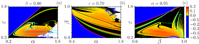
Figure 2: Global view of Lyapunov diagrams (parameter planes) of system (12) for (a) $(\alpha,\varepsilon)$, (b) $(\alpha,\beta)$, and (c) $(\beta,\varepsilon)$. Black color indicates null LLEs or periodic behavior, yellow to red one indicates positive LLEs or chaotic behavior (see the color bar in (c)). The white region indicates divergence while the blue one equilibrium points. Bifurcation curves are overlapped on the diagrams to characterize the positions where there exist specific bifurcations. The white box in (a) delimits the amplification region plotted in Fig. 3(a).

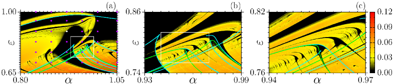
Figure 3: (a) Magnification of the white box in Fig. 2(a). Each magenta bullet plotted in this figure represents the parameter-pair used to obtain the experimental attractor projection (see Fig.  8) of system (12). (b) Magnification of the white box in Fig. 3(a) and, (c) white box in Fig. 3(b), respectively. The bifurcation curves are also overlapped on the diagrams. The left black region in (b), delimited by the cyan curve (saddle-node bifurcation) is an accumulation horizon where the stable periodic structures (better visualized in (c)), at right, accumulate themselves. The color scheme is shown in (c).

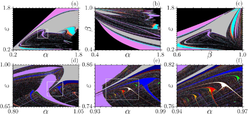
Figure 4: Isospike diagrams of system (12). Top row: (a)-(c) isospike diagrams of Fig. 2. Bottom row: (d)-(f) isospike diagrams of Fig. 3. The color scheme used is the following: violet for $q=1$, cyan for $q=2$, gray for $q=3$, coral for $q=4$, purple for $q=5$, dark-blue for $q=6$, red for $q=8$, dark-green for $q=10$, blue for $q=11$, dark-red for $q=12$, forest-green for $q=13$, yellow for $q=16$, white for $q=17$, orange for $q=21$, green for $q=23$, brown for $q=27$, magenta for $q=31$, and navy for $q=41$. Black represents other values of $q$, equilibrium points, chaos and divergences.

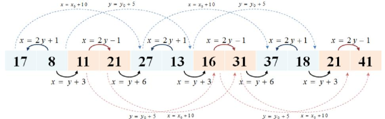
Figure 5: Schematic diagram showing the sequence of spikes observed in Fig. 4(f) and the organization rules of the structures obeying linear Diophantine equations, solid arrows (see the text), and spike-adding bifurcation cascades, dashed arrows. $x$ is the higher and $y$ is the lower number of spikes, $q$, of the pairs.

All the three projections $(\alpha,\beta)$, $(\alpha,\varepsilon)$, and $(\beta,\varepsilon)$, present some basic features, as portions of large periodic regions including SPSs embedded in chaotic domains. Large regions of equilibrium points are also observed as well as divergence regions. The bifurcation curves present a quite good agreement with the LLEs plotted in the Lyapunov diagrams and reveal the type of bifurcations that occur in the system for specific parameter-planes. In this case, we also can emphasize that such information about bifurcation neighborhoods is not accessed only by the LLEs. For example, the bifurcations between equilibrium points (blue domains) and periodic attractors (black domains) occur by Hopf bifurcations (see magenta curves) Hoff et al. [2014]; Dhooge et al. [2003] while the period-doubling bifurcations between two periodic attractors and, bifurcations between periodic attractors and chaotic ones occur by saddle-node bifurcations, illustrated by green and cyan curves, respectively.

The existence of SPSs embedded in chaotic domains is better visualized in the diagrams plotted in Fig. 3, that are magnifications of portions of Lyapunov diagrams of the white box in Fig. 2(a) and, show the presence of shrimp-shaped domains (stable-periodic-structures) organized themselves in some specific directions in Lyapunov diagrams as can be seen in Fig. 3(a). In Fig. 3(b), we show the magnification of the white box in (a), and in Fig. 3(c) the magnification of the white box in (b). The bifurcation curves are also showed in those diagrams, with green and cyan curves being period-doubling and saddle-node bifurcations, respectively. Regarding those set of bifurcation curves, it is worth to note four of them. The first is the cyan curve at the lowest right portion of the diagram in (a). This curve borders the right portion of a SPS of hook shape. In (b) we show that the curve delimits the accumulation horizon Bonatto & Gallas [2008], where the SPSs organizing themselves towards that periodic boundary. It is clear that in the accumulation horizon the bifurcations between the periodic and chaotic domains are saddle-nodes. The others three curves are shown in Fig. 3(c). They are the three curves overlapped the shrimp-shaped-domain in the center of the diagram. Those curves are two saddle-node and one period-doubling. In Ref. Hoff et al. [2013] the authors showed that the endoskeleton of a shrimp-shaped-domain is formed by four bifurcation curves, two saddle-node, and two period-doubling. Here, in (c), it was impossible to obtain the second period-doubling curve due to the numerical precision in the numerical continuation method Dhooge et al. [2003]; Barrio et al. [2011b, a]. But, it is clear the good agreement between the numerical integration (Lyapunov diagram) and continuation (bifurcation curves) methods.

Figure 6: Schematic circuitry implementation of the Watt governor model based on the set of Eqs. (12).

Figure 3(c) was plotted to study in more details the self-organization of the SPSs described in the paragraph above. Such SPSs organize themselves towards the periodic boundary, with the border delimited by a saddle-node bifurcation curve. Regarding this self-organization, we can associate to it the pattern of pairs of structures, and these pairs also organize themselves towards the periodic boundary. At this point, it is important to mention that a common self-organization of SPSs was previously reported in a large class of dynamical systems Celestino et al. [2014]; Gallas [2015]; da Costa et al. [2016]; Gallas [2016]; Hoff et al. [2013, 2014]; Cardoso et al. [2009]; Bonatto & Gallas [2008]. Specifically considering the sequence plotted in Fig. 3(c) we see that it is a period-adding sequence, where the SPSs organize themselves such that the number of spikes ($q$), in one period of the time series of the attractors related with these structures, increases by a constant factor along a specific direction. Furthermore, in the case reported in Fig. 3(c), we observe a peculiar sequence of accumulation where the number of spikes $q$ emerges organized according to a solution of integers of Diophantine equations. This is better explained in the following.

In Fig. 4 we present the isospike diagrams of system (12) in meshes of $1200\times 1200$ parameter values. Those diagrams are parameter-planes in which the number $q$ of spikes, in one period of time of the time-series, is used instead of LLEs, as in Figs. 2 and 3. The first row, Figs. 4(a)-(c), shows the isospike diagrams related to Fig. 2, and below, Figs. 4(d)-(f), the isospike diagrams of Fig. 3. The peculiar sequence of accumulation mentioned above, can be explained via those isospike diagrams. In Figs. 4(e) and (f), the pairs of SPSs are better visualized, for example, the white-red pair of structures with $q=(17;8)$, and the blue-orange pair with $q=(11;21)$, and so on, until to the accumulation boundary structure with $q=5$, the purple SPS at left in Fig. 4(e). Since the $q$ number of those structures is known, one can now analyze their organization rules. To make easier our analysis, Fig. 5 shows a schematic diagram with the pairs sorted in an inverse sequence as plotted in Fig. 4(f), where each pair represents a pair of SPSs in this same figure. The curved arrows with equations represent the organization rules of the SPSs’ spikes. Based on this diagram we suppose that there are at least four distinct rules for the organization of the SPSs, namely two rules for organization of the pairs, upper solid arrows in Fig. 5, and two rules connecting the distinct pairs, lower solid arrows in Fig. 5. The equations that represent the organization rules can be viewed as linear Diophantine equations. However, the two equations for organization of the spikes of distinct pairs can be described with only one equation, i.e., with the quadratic Diophantine equation $(x-2y)^{2}=1$, where $x$ and $y$ are the higher- and lower-spikes of the pairs, respectively. The two equations that connect the distinct pairs can also be described with only one quadratic Diophantine equation $(2x-2y-9)^{2}=9$. Therefore, with the two quadratic Diophantine equations it is possible to construct the whole accumulation sequence of SPSs towards the accumulation boundary. In this diagram, the spike-adding bifurcation cascades between alternated pairs become evident, i.e., between alternated solutions of the quadratic Diophantine equation $(x-2y)^{2}=1$, as represented by the upper and the lower dashed arrows. The equations for the spike-adding cascades indicate that we have a general solution for the spikes $x$ and $y$ given respectively by $x=x_{0}+2n$ and $y=y_{0}+n$, where $n=5$. To summarize this discussion it is essential to emphasize that the accumulation boundary of this sequence has $q=5$, as shown by Fig. 4(e).

We finish this Section stating the following partial conclusions: the dynamics of WGS, modeled by the set of Eqs. (12) in normalized and dimensionless variables, has a sensitive dependence of the combination of parameter values of $\epsilon$, $\alpha$ and $\beta$. As shown by our numerical results, depending on this parameter-set the WGS presents periodic (with high-spike values) and chaotic dynamics as shown respectively, by black and yellow up to red domains in Figs. 2 and 3. In a physical point of view, the mechanical WGS (shown in Fig. 1) presents periodic and chaotic motions depending on the choice of the three-parameter values. Besides, our results clearly show the existence of self-organized SPSs on parameter-space of the largest Lyapunov exponent and isospikes of time series of the WGS. In particular, a peculiar hierarchical organization and period-adding bifurcation cascade of the SPSs are observed and, they are accumulating on a periodic boundary (see Fig. 4). More interestingly, it is shown that the periods of these structures organize themselves obeying the solutions of Diophantine equations.

3 Experimental results

After an extensive numerical investigation about the dynamics of WGS, we also perform a quite interesting experimental study of same system, proposing an analog circuit implementation of system (12), as shown in Fig. 6. We start this Section describing the main devices used to construct the experimental setup as presented at next.

To construct the experimental setup it was used the following devices: (i) the operational amplifiers $TL074$ ($OP1A$,$\ldots$,$OP2A$,etc) to perform the addition, subtraction, and integration operations; (ii) the analog multipliers $AD633$ ($U1$,$U2$,$\ldots$) to implement the multiplications, and the trigonometric function converters $AD639$ ($A1$ and $A2$), to perform the trigonometric operations. In this circuitry implementation (of system (12)), the control parameters $\varepsilon$, $\alpha$ and, $\beta$ can be independently varied by adjusting the bias $V5$, $V3$, and $V6$, respectively. We have chosen vary bias Rocha & Medrano-T. [2009]; Medrano-T & Rocha [2014] instead of resistors de Sousa et al. [2016]; Tahir et al. [2016]; Viana et al. [2010, 2012], which are commonly used in circuitry implementations of dynamical systems, for a better fine tuning that we can obtain in the parameters. Besides, commercial and digital potentiometers are useful in some applications in which the signal-noise relation is not relevant, for instance, in linear systems. On the other hand, for nonlinear systems in which chaotic dynamics are significant, the signal-noise relation should be considered. As far as we know, commercial or home-made (as the digital de Sousa et al. [2016]) potentiometers, are noise sources in circuitry implementations, and in nonlinear dynamical systems, noise signal with a large enough strength may perturb the periodic attractors Viana et al. [2010, 2012], leading the system to chaotic motion. As presented bellow, the circuitry implementation of system (12) is highly noise-sensitive. Therefore, it is imperative to minimize the effects caused by sources of noise because, in this case, the system becomes experimentally more stable.

The bias sources (or the control parameters $\alpha$, $\varepsilon$ and, $\beta$) are controlled by the data acquisition ($DAQ$) board $NI$ $PCIe-6259$, by its analog outputs. In the measurements, we also use the $DAQ$ board, using three analog inputs (the variables $x$, $y$, and $z$). We used the Python ambient to control the $DAQ$ board measurements and also to analyze the data from time series with the TISEAN package Hegger et al. [1999].

After run a set of realizations, we plotted the experimental Lyapunov diagram in Fig. 7, obtained by the circuitry implementation of the system (12), in a resolution of $10^{2}\times 10^{2}$. The color scheme used is the same as discussed in Fig. 2: Black and yellow up to red colors for periodic and chaotic motions, respectively. This diagram is the experimental version of the diagram shown in Fig. 3(a). To obtain this experimental diagram, the circuit of Fig. 6 was built in a single-sided printed circuit board ($PCB$) driven by a $DC$ symmetric power-source, and connected to the $DAQ$ board, in the computer, by a block of $BNC$ connectors. Suitable home-made routines in Python ambient were developed to automate the measurements of the variables $x$, $y$, and $z$, and after to analyze the data using the routine lyap_spec from TISEAN package Hegger et al. [1999].

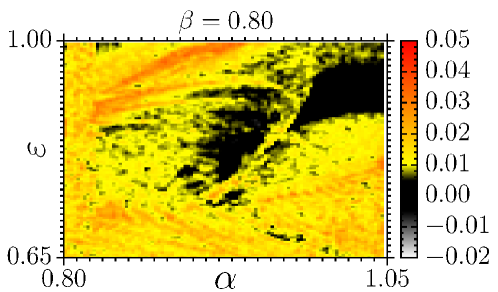
Figure 7: Lyapunov diagram of the circuitry implementation of the system (12). This diagram is the experimental version of the numerical diagram of Fig. 3(a). The color scheme for the LLEs is in the right-side palette.

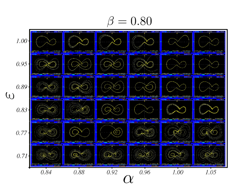
Figure 8: Each panel in this figure is an experimental attractor’s projection in the plane of variables $x\times y$ for the parameter pair highlighted by a magenta bullet in Lyapunov diagram of Fig. 3(a). The periodic attractors were obtained applying chaos control procedure (see the text) in some points of the experimental Lyapunov diagram of Fig. 7.

As shown and discussed elsewhere Viana et al. [2010, 2012]; Boccaletti et al. [2000], noise disturbs the basin of attractions of periodic attractors of nonlinear systems Manchein et al. [2013], usually inducing periodic behaviors to chaotic ones if the noise strength is high-enough, and specifically in the parameter-spaces, deforming and destroying the periodic structures Horstmann et al. [2017]. That effect is shown in Fig. 7 compared with the Fig. 3(a). We claim that noise in the circuitry implementation of Fig. 6 destroyed the smallest SPSs observed in Fig. 3(a) and deformed the two biggest ones: The central hook-shaped structure and the top-right periodic region, as shown in Fig. 7.

To reduce the noise effects in the circuit, and to control some chaotic domains that arise in the experimental Lyapunov diagram, we apply an effective chaos control procedure, as proposed in Ref. Boccaletti et al. [2000], in the circuitry implementation by adding a precision commercial potentiometer ($Rpot$ in Fig. 6) to stabilize the unstable periodic orbits (UPOs) embedded in the stable chaotic attractor for some set of parameters. With this procedure, we show in Fig. 8 an experimental diagram of some exemplary experimental attractors presenting the dynamics associated to the parameter-pairs highlighted by magenta bullets in Fig. 3(a) where this set of attractors is obtained by setting the circuit in certain values of parameters (each magenta bullet plotted in Fig. 3(a), is associated to an attractor in Fig.  8). To obtain such results it was necessary a manually fine tuning of the potentiometer, to stabilize the UPOs, as the attractors’ data were recorded directly from the digital oscilloscope by using print screen functionality. With this control, we are able to stabilize the experimental UPOs with the same number of spikes $q$, as shown in Fig. 4(d), from the chaotic orbits born from noise perturbations. For example, the periodic attractor for the parameter pair (illustrated by white bullet in Fig. 3(a)) $(\alpha,\varepsilon)=(0.92,0.89)$ in Fig. 8 has $q=5$ i.e. the same $q$ for the purple hook-shaped structure plotted in Fig. 4(d). Although the process, of manually fine tuning the potentiometer, used to stabilize the UPOs seems rough or imprecise, it was very useful as shown by the remarkable concordance between results plotted in Figs. 3(a) and 8, i.e bullets plotted on yellow up to red/black color regions in Fig. 3(a) related to chaotic/periodic attractors in Fig. 8. In addition, we also show in this exemplary set of panels how the dynamics of the mechanical WGS (in which the dynamics is reproduced by an electronic circuit) changes (from periodic to chaotic or vice-versa) when at least one control parameter is varied.

The second set of partial conclusions is based on a rich and complex dynamics presented by the quite interesting experimental study of WGS through of analog circuit implementation of system 12, as shown in Fig. 6. In this circuitry implementation, the control parameters $\epsilon$, $\alpha$ and, $\beta$ can be independently varied by adjusting bias in the circuit. After a set of experimental realizations we plotted the experimental Lyapunov diagram, which is in agreement with the theoretical counterpart. We also applied an effective chaos control procedure, as proposed in Ref. Boccaletti et al. [2000], in the circuitry implementation by adding a precision commercial potentiometer (Rpot in Fig. 6) to stabilize the unstable periodic orbits (UPOs) embedded in the stable chaotic attractor for some sets of parameters.

4 Summary and conclusions

In this work we carried out extensive numerical and experimental studies in a model of the Watt governor system (WGS). We start to investigate the dynamics of WGS applying a numerical approach to characterize the presence of generic stable periodic structures (SPSs) embedded in chaotic domains of the three-dimensional parameter-space of system 12. Numerical results corroborate with the generic nature of those SPSs, independently of the systems’ nonlinearity. Using the numerical continuation method to solve the same system we characterize the Hopf, period-doubling and saddle-node bifurcation curves, as plotted in the parameter planes of Figs. 2 and 3. Comparing the position of such curves in these Lyapunov diagrams with the results shown in the isospike diagrams (see Fig. 4) it is possible to realize the remarkable concordance between such results, even if the invariant measure used in each case is different. We also discuss how the SPSs organizes themselves in some preferred directions on the Lyapunov and isospike diagrams of the WGS model (see Eqs. (12)). We characterize a new hierarchical organization of these SPSs, where the periods follow the solutions of Diophantine equations. It is worth to mention that in other portions of the Lyapunov diagrams we detected sequences of structures which periods are self-organized following the solutions of Diophantine equations. To the best of our knowledge, the numerical results reported here, through the Lyapunov and spike diagrams, are difficult (maybe impossible) to be analytically predicted. One open question that deserves further studies is what sorts of systems present the hierarchical organization shown here, i.e., following the solutions of Diophantine equations.

To test the robustness of our numerical results an experimental setup was implemented by a circuitry analogy of mechanical systems using an analog computing technique. After applying an active control of chaos in the experiment, the effect of intrinsic experimental noise was minimized such that, the experimental results are in astonishing well agreement with our numerical findings. Another interesting result obtained from our experimental approach is related to the application of analog computing technique to mechanical problems that can be used to obtain experimental results from different real problems.

Acknowledgments The authors thank Conselho Nacional de Desenvolvimento Científico e Tecnológico (CNPq), Coordenação de Aperfeiçoamento de Pessoal de Nível Superior (CAPES), Fundação de Amparo à Pesquisa e Inovação do Estado de Santa Catarina (FAPESC), Brazilian agencies, for financial support.

References

- Barrio et al. [2011a] Barrio, R., Blesa, F., Dena, A. & Serrano, S. [2011a] “Qualitative and numerical analysis of the Rössler model: Bifurcations of equilibria,” Comput. Math. Appl. 62, 4140.
- Barrio et al. [2011b] Barrio, R., Blesa, F., Serrano, S. & Shilnikov, A. [2011b] “Global organization of spiral structures in biparameter space of dissipative systems with Shilnikov saddle-foci,” Phys. Rev. E 84, 035201(R).
- Boccaletti et al. [2000] Boccaletti, S., Grebogi, C., Lai, Y., Mancini, H. & Maza, D. [2000] “Control of chaos: theory and applications,” Phys. Rep. 329, 103.
- Bonatto & Gallas [2008] Bonatto, C. & Gallas, J. A. [2008] “Accumulation boundaries: Codimension-two accumulation of accumulations in phase diagrams of semiconductor lasers, electric circuits, atmospheric, and chemical oscillators,” Phil. Trans. R. Soc. A. 366, 505.
- Cardoso et al. [2009] Cardoso, J. C. D., Albuquerque, H. A. & Rubinger, R. M. [2009] “Complex periodic structures in bi-dimensional bifurcation diagrams of a RLC circuit model with a nonlinear NDC device,” Phys. Lett. A 373, 2050.
- Celestino et al. [2011] Celestino, A., Manchein, C., Albuquerque, H. A. & Beims, M. W. [2011] “Ratchet transport and periodic structures in parameter space,” Phys. Rev. Lett. 106, 234101.
- Celestino et al. [2014] Celestino, A., Manchein, C., Albuquerque, H. A. & Beims, M. W. [2014] “Stable structures in parameter space and optimal ratchet transport,” Commun. Nonlinear Sci. Numer. Simulat. 19, 139.
- da Costa et al. [2016] da Costa, D. R., Hansen, M., Guarise, G., Medrano-T, R. O. & Leonel, E. D. [2016] “The role of extreme orbits in the global organization of periodic regions in parameter space for one dimensional maps,” Phys. Lett. A 380, 1610.
- de Sousa et al. [2016] de Sousa, F. F. G., Rubinger, R. M., Sartorelli, J. C., Albuquerque, H. A. & Baptista, M. S. [2016] “Parameter space of experimental chaotic circuits with high-precision control parameters,” Chaos 26, 083107.
- Dhooge et al. [2003] Dhooge, A., Govaerts, W. & Kuznetsov, Y. A. [2003] “Matcont: a Matlab package for numerical bifurcation analysis of ODEs,” ACM Trans. Math. Softw. 29, 141.
- Gallas [2015] Gallas, J. A. C. [2015] “Periodic oscillations of the forced Brusselator,” Mod. Phys. Lett. B 29, 1530018.
- Gallas [2016] Gallas, J. A. C. [2016] “Systematics of spiking in some CO2 laser models,” Advances in Atomic, Molecular, and Optical Physics, eds. Arimondo, E., Lin, C. C. & Yelin, S. F., “3,” (Elsevier Science), pp. 127–191.
- Hegger et al. [1999] Hegger, H., Kantz, H. & Schreiber, T. [1999] “Practical implementation of nonlinear time series methods: The TISEAN package,” Chaos 9, 413.
- Hills [1989] Hills, R. L. [1989] Power from Steam: A history of stationary steam engine (Cambridge University Press, Cambridge).
- Hoff et al. [2013] Hoff, A., da Silva, D. T., Manchein, C. & Albuquerque, H. A. [2013] “Bifurcation structures and transient chaos in a four-dimensional Chua model,” Phys. Lett. A 378, 171.
- Hoff et al. [2014] Hoff, A., dos Santos, J. V., Manchein, C. & Albuquerque, H. A. [2014] “Numerical bifurcation analysis of two coupled FitzHugh-Nagumo oscillators,” Eur. Phys. J. B 87, 151.
- Horstmann et al. [2017] Horstmann, A. C. C., Albuquerque, H. A. & Manchein, C. [2017] “The effect of temperature on generic stable periodic structures in the parameter space of dissipative relativistic standard map,” Eur. Phys. J. B 90, 96.
- MacFarlane [1979] MacFarlane, A. G. J. [1979] “The development of frequency-response methods in automatic control,” IEEE T. Automat. Contr. AC-24, 250.
- Manchein et al. [2013] Manchein, C., Celestino, A. & Beims, M. W. [2013] “Temperature resistant optimal ratchet transport,” Phys. Rev. Lett. 110, 114102.
- Maxwell [1868] Maxwell, J. C. [1868] “On governors,” Proc. Roy. Soc. London 16, 270.
- Medrano-T & Rocha [2014] Medrano-T, R. O. & Rocha, R. [2014] “The negative side of Chua’s circuit parameter space: Stability analysis, period-adding, basin of attraction metamorphoses, and experimental investigation,” Int. J. Bifurc. Chaos 24, 1430025.
- Meucci et al. [2016] Meucci, R., Euzzor, S., Pugliese, E., Zambrano, S., Gallas, M. R. & Gallas, J. A. C. [2016] “Optimal phase-control strategy for damped-driven Duffing oscillators,” Phys. Rev. Lett. 116, 044101.
- Pontryagin [1962] Pontryagin, L. S. [1962] Ordinary Differential Equations (Addison-Wesley Publishing Company Inc.).
- Rech [2016] Rech, P. C. [2016] “Quasiperiodicity and chaos in a generalized Nosé–Hoover oscillator,” Int. J. Bifur. Chaos 26, 1650170.
- Rocha & Medrano-T. [2009] Rocha, R. & Medrano-T., R. O. [2009] “An inductor-free realization of the Chua’s circuit based on electronic analogy,” Nonlinear Dyn. 56, 389.
- Schmidt [1991] Schmidt, W. M. [1991] Diophantine Approximations and Diophantine Equations (Springer-Verlag).
- Silva et al. [2015] Silva, S. L. d., Viana, E. R., Oliveira, A. G. d., Ribeiro, G. M. & Silva, R. L. d. [2015] “High resolution parameter-space from a two-level model on semi-insulating GaAs,” Int. J. Bifurc. Chaos 25, 1530004.
- Sotomayor et al. [2007] Sotomayor, J., Mello, L. F. & Braga, D. C. [2007] “Bifurcation analysis of the Watt governor system,” Comp. Appl. Math. 26, 19.
- Strogatz [2001] Strogatz, S. H. [2001] Nonlinear Dynamics and Chaos:With Applications to Physics, Biology, Chemistry, and Engineering (Westview Press).
- Tahir et al. [2016] Tahir, F. R., Ali, R. S., Pham, V., Buscarino, A., Frasca, M. & Fortuna, L. [2016] “A novel 4d autonomous 2n-butterfly wing chaotic attractor,” Nonlinear Dyn. 85, 2665.
- Viana et al. [2010] Viana, E. R., Rubinger, R. M., Albuquerque, H. A., de Oliveira, A. G. & Ribeiro, G. M. [2010] “High-resolution parameter space of an experimental chaotic circuit,” Chaos 20, 023110.
- Viana et al. [2012] Viana, E. R., Rubinger, R. M., Albuquerque, H. A., de Oliveira, A. G. & Ribeiro, G. M. [2012] “Periodicity detection on the parameter-space of a forced Chua’s circuit,” Nonlinear Dyn. 67, 385.
- Zhang et al. [2010] Zhang, G., Mello, L. F., Chu, Y. D., Li, X. F. & An, X. L. [2010] “Hopf bifurcation in an hexagonal governor system with a spring,” Commun. Nonlinear Sci. Numer. Simulat. 15, 778.