Improving Retrieval Modeling Using Cross Convolution Networks And Multi Frequency Word Embedding

Abstract

To build a satisfying chatbot that has the ability of managing a goal-oriented multi-turn dialogue, accurate modeling of human conversation is crucial. In this paper we concentrate on the task of response selection for multi-turn human-computer conversation with a given context. Previous approaches show weakness in capturing information of rare keywords that appear in either or both context and correct response, and struggle with long input sequences. We propose Cross Convolution Network (CCN) and Multi Frequency word embedding to address both problems. We train several models using the Ubuntu Dialogue dataset which is the largest freely available multi-turn based dialogue corpus. We further build an ensemble model by averaging predictions of multiple models. We achieve a new state-of-the-art on this dataset with considerable improvements compared to previous best results.

1 Introduction

One of the primary objectives in Artificial Intelligence (AI) is the task of building a conversational agent that can naturally and coherently communicate with humans. The solution can significantly change the interaction between clients and customers, and has appealing applications to service providers in many different areas. This task can be simplified to define different problems whose solutions move us toward accurate understanding and modeling of human conversation. The two mainstream models can be distinguished as follows: a Generative model that tries to generate responses in multi-turn conversations Sordoni et al. (2015); Wen et al. (2015b, a); Shang et al. (2015), and a Retrieval model which retrieves potential responses from the massive repository and selects the best one as the output Yan et al. (2016); Ji et al. (2014). While the first model is a more flexible and powerful model, it is considerably harder to implement. According to the current state of AI, we are far away from a generative model for long and multi-domain conversations.

Until recently, proposed solutions for building dialogue systems required significant hand-engineering of features. This limits the number of responses and situations in which the system can be deployed. More recently, researchers tempt to apply machine and deep learning methods to create a model that can learn the essential information in conversational data. One vital aspect of human conversation is the contextual and semantic relevance among sentences. The sequence modeling approaches are shown to be effective to capture these information. More specifically, Recurrent Neural Networks (RNN) built by Long Short-Term Memory (LSTM) units Hochreiter and Schmidhuber (1997) have been effectively utilized for extracting contextual and semantic information in other language related problems such as speech recognition, state tracking, image captioning, etc. Sutskever et al. (2014); Cho et al. (2014); Henderson et al. (2013); Graves et al. (2013); Xian and Tian (2017).

In this paper, we consider the problem of next response ranking for multi-turn human-computer conversation with a given context. The model provides candidates’ ranking and selects the one with the highest rank as the next utterance. This problem is an important and challenging task for the retrieval-based dialogue model.

Previous RNN based approaches to response selection take the context and the response candidate as two separate word sequences and feed them to the RNN in order to obtain two embedding vectors. The response is then selected based on the similarity of the candidate embedding with the context embedding Lowe et al. (2015); Kadlec et al. (2015); Baudiš et al. (2016); Xu et al. (2016). There are mainly two shortcomings of previous solutions. The first shortcoming corresponds to the method of representing words in the context and candidates. More specifically, in order to efficiently represent words of either the context or the response and feed them to the RNN, we use word vector embeddings. A word embedding is a vector which represents word’s semantic and synthetic features. Intuitively, we map words to $N$-dimensional vectors, where vectors that are relatively close represent words with similar or related meaning Mikolov et al. (2013). However, in order to have sufficient semantic and syntactic information for a word, and also to make this method computationally efficient, we require the word to appear in the corpus for at least a certain number of times. Hence, rare words, which are usually technical words and carry important information, are missed by such word embedding method. The second shortcoming relates to the performance of RNN. In fact, LSTM units are vulnerable to losing information when the input sequence is long (which is the case in multi-turn response selection. See Section 2). Furthermore, in the RNN based models, the inputs to the RNN are the sequence of word embeddings of the entire context (or response), and the output is a single vector which represent the contextual and semantic dependency and relevance of the words in the entire context (or response) and does not carry word level information. To address the first problem, we utilize two word embedding layers: one for frequent words and one for rare words. To address the second issue, we extract the similarity between individual words in the context and the response. We note that when an utterance shares a rare word with some context, it is more probable that it is the correct response for the context. Therefore, we design a layer to extract the information of rareness of shared words in the context and the response.

In this paper, we propose a model that integrates sequence and word level information. We train our model on the Ubuntu Dialogue dataset, which consists of roughly one million two-way conversations extracted from the Ubuntu chat logs. Moreover, this data set is considered to be unstructured dialogues where there is no a priori logical representation for the information exchanged during the conversation Lowe et al. (2017) which is a desirable property to test a retrieval model.

We summarize our contributions as follows:

• We design Cross Convolution Network (CCN) that gets two inputs (matrix representations of two sentences, feature matrices of two images, etc.) and extracts similarity of the inputs.

• We propose Multi Frequency Word Embedding that efficiently capture both frequent and rare words of the corpus.

• Our experimental results show a considerable improvement over previous results on Ubuntu Dialogue Corpus Lowe et al. (2015).

The remainder of this paper is structured as follows. In Section 2, we review previous work. Description of the dataset can be found in Section 3. In Section 4, we present our methods to capture sequence level and word level information in detail. Section 5 focuses on the experimental setup while our results are presented in Section 6. Finally, We conclude and discuss future research directions in Section 7.

2 Related Work

The problem of next response selection in multi-turn conversation is more general than a traditional question answering (QA) problem Yih et al. (2015); Yu et al. (2014). The prediction is made based on the entire conversation context which does not necessarily include a question. In single turn response selection, the model ignores the entire context and only leverages the last utterance to select response Lu and Li (2013); Ji et al. (2014); Wang et al. (2015). Since an utterance can change the topic or negate/affirm the previous utterances, it is of paramount importance that models for response selection in multi-turn conversation have a certain understanding of the entire context. Moreover, next response selection system is a supervised dialogue system since it incorporates explicit signals specifying whether the provided response is correct or not Lowe et al. (2016). This system is of interest because it admits a natural evaluation metric, namely the recall and precision measures (See Section 3 for a detailed explanation.). We consider Ubuntu Dialogue Corpus Lowe et al. (2015) to evaluate our retrieval-based model since the dataset is the most relevant public dataset to supervised dialogue systems Lowe et al. (2016).

The original paper that introduced the Ubuntu Dialogue dataset have implemented a TF-IDF model in addition to neural network models with vanilla RNN and LSTM Lowe et al. (2015). Later, Kadlec et al. (2015) evaluated the performances of various LSTMs, Bi-LSTMs and CNNs (Convolutional Neural Networks Kalchbrenner et al. (2014)) on the dataset and created an ensemble by averaging predictions of multiple models. An RNN-CNN model combined with attention vectors is implemented by Baudiš et al. (2016). Further, Multi-view Response Selection Zhou et al. (2016) proposed an RNN-CNN model which integrates information from both word sequence view and utterance sequence view. A deep learning model incorporating background knowledge to enhance the sequence semantic modeling ability of LSTM is implemented in Xu et al. (2016) that achieved the state-of-the-art result.

In spite of these efforts, the study of Lowe et al. (2016) found that the automated dialogue systems built using machine and deep learning methods perform worse than human experts in Ubuntu system. This confirms that further investigation in retrieval dialogue system using this dataset is worthwhile and motivates us to conduct this research.

3 Data

The Ubuntu Dialogue Corpus Lowe et al. (2015) is the largest freely available multi-turn based dialogue corpus which consists of almost one million two-way conversations extracted from the Ubuntu chat logs. We use the second version of this dataset in this paper. The dataset was preprocessed as follows:

• Named entities were replaced with corresponding tags (name, location, organization, url, path).

• Two special symbols; namely, $eou$ and $eot$ are used to denote the end of utterances and turns, respectively.

• The training set consists of tuples of the form $<$$context,response,label$$>$, where the $label$ indicates whether the provided $response$ is the correct response for the $context$ or not. For any instance of the form $<$$context,response,1$$>$, the set includes an instance of the form $<$$context,response^{\prime},0$$>$ where the $response^{\prime}$ is a randomly sampled utterance from the entire data to create balanced dataset.

• The test set is created by $2\%$ of the whole dataset which is approximately 20k instances. Each test instance consists of a $context$ followed by 10 candidate responses with the first candidate being the correct one. The other $9$ responses are drawn randomly from the entire corpus Lowe et al. (2015). Furthermore, a validation set of the same size and structure is provided.

The system is required to rank the candidate responses and output the highest ranking. We note that some of the sampled candidates which are labeled as incorrect can be relevant to the context, and hence, considered as correct. Hence, we may examine the system’s ranking as correct if the correct response is among the first $k$ candidates. This quantity is denoted by $Recall@k$. Most of the previous papers have used the pairs of $(m,k)$ to be $(10,1)$, $(10,2)$, and $(10,5)$ to report their models’ performance Lowe et al. (2015); Zhou et al. (2016); Kadlec et al. (2015).

4 Method

In this section, we provide details on the networks and layers we used to build our models. We start by introducing the Cross Convolution Network that captures semantic similarity of the context and response. We then elaborate on Multi Frequency Word Embedding. It is followed by explanation of LSTM network and Common Words Frequency layer.

4.1 Cross Convolution Network

In many instances, a handful number of words reveal the purpose of conversation; therefore, one may expect to see the exact same words in the context or their derivations in the correct response. Our experiments show that RNN models fall short of capturing all these information especially when the input sequence is long. Motivated by this, we design a Cross Convolution Network that intrinsically can be deployed in any classifying problem of a pair of objects. We would like to mention that CCN is different with the architecture proposed in Wan et al. (2016) which utilizes Bi-LSTM and requires to learn parameters of an interaction tensor to capture semantic matching of two sentences.

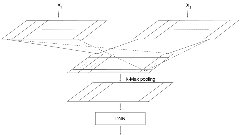
Figure 1: Cross Convolution Network (CCN). $X_{1}$ and $X_{2}$ are the inputs to the network. CCN computes convolution of $X_{1}$ over $X_{2}$ and passes the output result to a $k$-Max Pooling to extract the first k largest output of each column. A dense layer is then applied to calculate a number that measures similarity of $X_{1}$ and $X_{2}$.

At a high level, a Cross Convolution Network accepts two matrices, $X_{1}$ and $X_{2}$, and computes convolution of $X_{2}$ over $X_{1}$. $k$-Max Pooling is then applied to the output matrix in order to take the $k$ largest element of each of its column. The output is then fed to a Dense layer (vanilla RNN) that measures similarity of $X_{1}$ and $X_{2}$. As in Convolutional Neural Network, we need to specify the window and stride sizes for computing the convolution of inputs. Figure 1 shows structure of Cross Convolution Network.

For the task of response selection, we include the following layers to extract the word level information in the context and in the corresponding response:

Dot Product Layer Given the sequence of embedded word vectors of a context and a response, for each word $w_{r}$ in the response, we calculate its inner product with every word $w_{c}$ in the context. In other words, we calculate convolution of the context with each of the response words (as Convolutional filter) while window and stride sizes are equal to one.

$\bf k$-Max Pooling and Dense Layer Given the output of the Dot Product Layer, we pick the first $k$ maximum values for each filter $w_{r}$. We then use a dense layer (DNN with some activation function) to calculate the probability of the corresponding label of the instance to be one.

In matrix representation of the context and response, in which the $i$-th column of the context (response) matrix is the embedding vector representing the $i$-th word in the context (response), we formulate the layer operation as

$$S =[S_{1},S_{2},\dots,S_{L}]=R^{T}C,$$ (1)

$$\bar{S}_{i} =kmax(S_{i}),$$

$$s_{3} =a^{T}\times[\bar{S}_{1};\bar{S}_{2};\dots;\bar{S}_{L}]+b,$$

$$p_{3} =f(s_{3}),$$

where $R$ is the response matrix, $C$ is the context matrix, and $S$ is the dot product output. $kmax(\cdot)$ is $k$-Max Pooling function which picks the first $k$ maximum values of each of the column of matrix $S$. Moreover, $a$ and $b$ are trainable weight vector and bias of the dense layer, respectively. $f(\cdot)$ can be any activation function. $k$ is a hyper-parameter for the model, and $L$ is the maximum number of words in the contexts and responses (the smaller contexts and responses are padded using zero vectors.).

4.2 Multi Frequency Word Embedding

To have high quality representation of words that capture syntactic and semantic word relationships, we use two types of word embedding layers in our models. As noted in Lowe et al. (2017), failure of understanding semantic similarity of context and response is the largest source of error from Dual-LSTM model (see Section 4.3). We observed that our dual LSTM model performed worse when rare words appeared in either or both context and response. One potential explanation is that when training the word embeddings, rare words are removed for the purpose of computational efficiency. However, this weakens the word embeddings due to the loss of information that occurs by ignoring rare words. In order to capture these rare word relation, we utilize multiple word embedding layers instead of one, we attempt to use two word embedding layers, which we refer to as low frequency, and high frequency layers.

Given the word sequences of context and response, words are mapped into $N$-dimensional embedding vectors. While $N$ is a hyper-parameter and needs to be specified, the word embeddings can be initialized with random vectors or with pre-trained word vectors. We use two independent word embedding layers inside a single model. First, we count total appearance of each word in train set of context and response, then filter frequent words and rare words during training from each context and response. The high frequency word embedding layer is the same as the word embedding of Lowe et al. (2015), which captures word relation of frequent words and feed to LSTM in future stage to get internal representation of context and response. The low frequency word embedding layer is trained using only rare words from train set of context and response. We denote the high frequency word filter, low frequency word filter, and embedding layer by $HFWF(\cdot)$, $LFWF(\cdot)$ and $WE(\cdot)$, respectively. Therefore,

$$WE_{h}=WE(HFWF(contexts\cup responses))$$ (2)

$$WE_{l}=WE(LFWF(contexts\cup responses)),$$

where $WE_{h}$ ($WE_{l}$) is the corresponding word embeddings for high (low) frequency word embedding layer that is train on high (low) frequency words in the entire training set.

4.3 LSTM

4.3.1 Context and Response Embedding

Long Short-Term Memory (LSTM) is well known for capturing information of long sequences. Inspired by Lowe et al. (2015), we use two LSTM networks with shared weights to produce the final representation of context and response by feeding word embeddings one at a time to the respective LSTM. Word embeddings are initialized using the pre-trained $300$-dimensional GloVe Word Vector Model Pennington et al. (2014), and updated during training phase. We use one hidden layer for each LSTM with output size $256$. We denote the LSTM layer by $LSTM(.)$. Therefore,

$$c=LSTM(WE(context))$$ (3)

$$r=LSTM(WE(response))$$

where $c$ and $r$ are the final hidden state of LSTM layer. We refer to this model as Dual-LSTM. This is the baseline model proposed in Lowe et al. (2015) where the response is then selected based on the similarity of $c$ and $r$ which is measured by the inner product of the two embeddings.

Finally, we dense the hidden state of LSTM layer, and calculate the probability of the response to be the correct one. More precisely, we compute the following:

$$s_{1} =c^{T}\times M\times r$$ (4)

$$p_{1} =sigmoid(s_{1})$$

where $M$ is a trainable weight matrix.

4.3.2 Common Words Embedding

Another issue raised by Lowe et al. (2017) is that direct word copying between the context and true response was not captured by Dual-LSTM model. In order to overcome this issue, we extract common word list from context and response, and feed common word embeddings to the LSTM network. We use the same word embedding layer as the other inputs of the Dual-LSTM model.

$$Common=LSTM(WE(context\cap response))$$ (5)

Finally, we dense the hidden state of LSTM layer, and calculate the score of the corresponding response to be correct.

$$s_{2}=d^{T}\times Common,$$ (6)

where $d$ is a trainable weight vector.

In the case of having both embedding layers, we concatenate the scores of common word embedding layer and Dual-LSTM layer and using sigmoid function to calculate the probability of the response to be the correct one:

$$p_{2}=sigmoid(\alpha_{1}s_{1}+\alpha_{2}s_{2})$$ (7)

where $\alpha_{1}$ and $\alpha_{2}$ are trainable weights.

4.4 Context-Response Common Words Frequency

This is a well-known fact that words which are more frequent (such as the, is, and that) contain less information compared to more rare words (such as technical words in Ubuntu Corpus). We observe that when an utterance shares a rare word with some context, it is more probable that it is the correct response for the context. To capture this, we first create a table that stores word occurrence count. We use this table to calculate a variable that is the summation over reciprocal of common words’ occurrences in a context and a response. More precisely; denoting by $n_{w_{i}}$ the number of times that word $w_{i}$ appeared in train dataset, for any context and response, we define $s(context,response)$ as follows:

$$s(context,response)=\sum_{i:w_{i}\in cr}\frac{1}{n_{w_{i}}},$$ (8)

where $cr=context\cap response$.

We note that unlike the TF-IDF model that computes TF-IDF vectors of both the context and the response and calculates the cosine similarity between the two vectors, our proposed layer only considers common words in the context and the response and is intended to reflect how informative a common word in context and response is.

5 Experiment

In this section, we provide details on our experiments including data preparation, experimental settings, the models we build using the networks and layers introduced in Section 4, and training parameters and functions.

5.1 Data Preparation

We preprocessed the ubuntu dataset by normalizing every context and response using TweetMotif O’Connor et al. (2010). We use the tokenization function of TweetMotif to treat hashtags, @-replies, abbreviations, strings of punctuation, emoticons and unicode glyphs (e.g., musical notes) as tokens. In order to reproduce the original result, we kept all the train, validation, and test sets same as the original sets provided by Lowe et al. (2015).

5.2 Experimental Setting

The experiment was executed on Amazon AWS p2 xlarge machine with NVIDIA Tesla K80 GPU. We use Keras Chollet et al. (2015) to implement all our models. All models were trained using Root Mean Square Propagation optimizer (RMSProp) Hinton et al. (2012) with learning rate set to $10^{-3}$ without decay. Also, the batch size is set to $256$ during training.

5.3 Model Training

We trained two different models with combination of few methods:

• Apply Multi Frequency Word Embedding and Common Word Embedding to LSTM structure. We refer to this model as MFCW-LSTM. Figure 2 depicts the model.

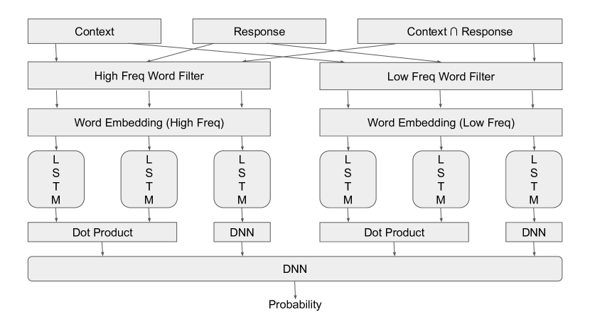
Figure 2: Diagram of MFCW-LSTM model. $Context\cap Response$ is the list of common words between context and response pair. Every single word in Context, Response, $Context\cap Response$ is filtered by High Frequency Word Filter $(>5)$ and Low Frequency Word Filter $(\leq 5)$, then feed to low frequency word embedding layer and high frequency word embedding layer, respectively. All the embedded results are fed into the correspond LSTM word-by-word. The LSTMs have tied weights for output of each word embedding layer respectively.

• Implement Cross Convolution Network and LSTM structure. High frequency layer of word embedding is the only embedding we use here. We refer to this model as CCN-LSTM. Figure 3 depicts the model.

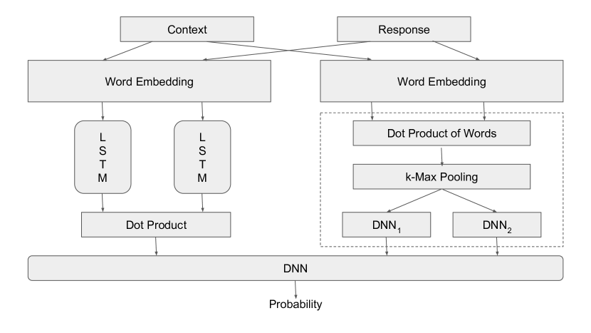
Figure 3: Diagram of CCN-LSTM model. The LSTMs have tied weights, and the two word embedding layers do not share weights. The dashed box is the Context-Response Words Relation networks with Dot Product, k-Max Pooling, and Dense layers.

All LSTM structures have $256$ hidden units. The maximum size of the context and response is set to $160$ words plus zero padding. The word embedding size is $300$ as in GloVe embedding.

For MFCW-LSTM, we tried different thresholds for high and low frequency word boundary, and found $5$ is the best threshold. We also learned parameters of LSTM with both shared weights and separate weights. For CCN-LSTM, we used two separated word embedding layers to feed words to the Context-Response Words Relation and LSTM networks. Parameter $k$ is set to $1$ and $2$ for different models; however, we did not see any improvement in models with $k=2$ over models with $k=1$.

To predict the label of a response for a context during training phase, we consider weighted sum of the response scores calculated by each of the networks in the considered model and apply sigmoid function that yields a number between $0$ and $1$. We then penalize the predicted label using square error loss function. The Context-Response Common Words Frequency layer is not used in the models during training. We discuss this issue more in the Result Section (Section 6).

5.4 Ensemble

Ensemble of multiple models can help us obtain better predictive performance than what we can get from any of the constituent models Opitz and Maclin (1999); Polikar (2006); Sollich and Krogh (1996). Similar to Kadlec et al. (2015), we found that averaging the prediction result of multiple models gives a decent improvement. We found that the best classifier is ensemble of 16 MFCW-LSTMs and 4 CCN-LSTMs.

6 Result

In this section we provide our experiments result in two subsections. Firstly, we report our models’ performance and discuss the results. Afterwards, we provide comparison of our best model performance with previous work’s.

6.1 Evaluation

We use the same evaluation metric as Lowe et al. (2015), namely $Recal@k$. Among $m=10$ response candidates provided in evaluation and test set, $1$ positive and $9$ negative responses are used. The model ranks $10$ responses, and prediction is considered correct if the correct response is in top $k$ candidates. we are reporting with $(m,k)$ of $(10,1)$, $(10,2)$ and $(10,5)$.

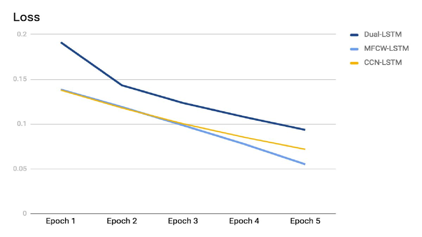
Figure 4: Loss change for validation set.

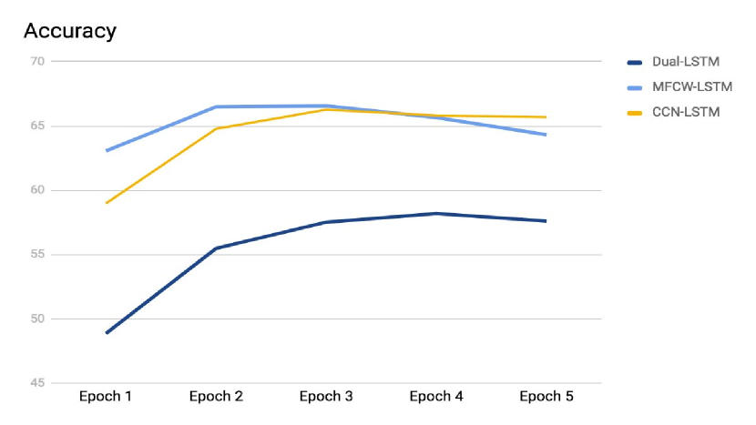
Figure 5: Accuracy change for validation set. We found accuracy start decreasing after third epoch for various models.

We choose the best models using the accuracy on validation set (Figure 4 and Figure 5). The performance of these models on test set are reported in Table 1. We reproduce the result of Dual-LSTM model as our baseline Lowe et al. (2015), and compare our models to this. We use same default hyper-parameter setting for Dual-LSTM as our other models, and initialize word embedding using Glove word vector Pennington et al. (2014). The reproduced performance of Dual-LSTM model in here is better than original result Lowe et al. (2017) since we are using high frequency word embedding and preprocessed dataset.

MFCW-LSTM and CCN-LSTM are the models described in Subsection 5.3. The CCN-LSTM model has $k=1$ and two dense parallel layers of linear and sigmoid in Context-Response Words Relation network as in Figure 3. Both of these models outperform Dual-LSTM model by approximately 9%. We also incorporate the MFCW-LSTM and CCN-LSTM to a single model, and the result is not better than any one of two.

We now investigate the effect of Context-Response Common Words Frequency (see Subsection 4.4 for details.) in response prediction. The scaled scores computed using Equation 8 are added to the resulting probabilities out of MFCW-LSTM and CCN-LSTM models in validation and test. Particularly, in order to predict the correct response on validation and test dataset, we first compute the score for each of the ten candidates responses using our model. After that we calculate $s(context,response)$ for each response, scale it, and add it to the model output. We then rank the responses based on this final score and choose the highest ranking as output. The scaling factor is optimized on the validation set. The combined models’ results can be found in the MFCW-LSTM-CWF and CCN-LSTM-CWF rows (Table 1), where CWF stands for common words frequency. As we can see, CWF layer improve performance of both baseline models of MFCW-LSTM and CCN-LSTM. We see a noticeable improvement for CCN-LSTM which can be attributed to the fact that CCN-LSTM model does not include rare words in its decision.

Table 1: Result of our models on Ubuntu Dialogue Corpus test set for different recall measures. Numbers in bold is our best model performance.

Model	1 in 10R@1	1 in 10R@2	1 in 10R@5
LSTM	57.6%	75.3%	94.5%
MFCW-LSTM	66.5%	80.4%	95.4%
CCN-LSTM	66.3%	80.8%	95.6%
MFCW-LSTM-CWF	67.3%	81.2%	95.6%
CCN-LSTM-CWF	69.0%	82.2%	96.0%
Ensemble	72.7%	85.8%	97.1%

Table 2: Performance comparison of our best models and different recent papers. Numbers in bold mean that the improvement is statistically significant compared with previous baseline.

Model	1 in10R@1	1 in10R@2	1 in10R@5
Dual-LSTM Lowe et al. (2017)	55.2%	72.1%	92.4%
RNN-CNN Baudiš et al. (2016)	67.2%	80.9%	95.6%
r-LSTM Xu et al. (2016)	64.9%	78.5%	93.2%
Ensemble Kadlec et al. (2015)	68.3%	81.8%	95.7%
SMN Wu et al. (2017)	72.6%	84.7%	96.2%
Our Best Model	72.7%	85.8%	97.1%

6.2 Comparison

Table 2 shows performance comparison of our best models and different recent papers. Since we used the Ubuntu Dialogue Corpus v2 dataset, and we compare our result to other works based on the same version. Recently, Wu et al. (2017) achieved decent improvement over the previous state-of-the-art. As we can see our best model which is the ensemble model outperforms SMN Wu et al. (2017) by $0.1\%$, $1.1\%$, and $0.9\%$ for 1 in10R@1, 1 in10R@2, and 1 in10R@5 metrics, respectively (Table  2). Therefore, we set a new state-of-the-art to 72.7%, 85.8% and 97.1%.

7 Conclusion and Future Work

In this paper, we considered the problem of next response selection for multi-turn conversation. Motivating by the large gap between machine and expert performances on this task for Ubuntu Dialogue Corpus, we presented new networks and layers and we evaluated our models using this dataset. We proposed Cross Convolution Network (CCN) that is potentially useful for the general task of classifying a pair of objects. We implemented CCN combined with LSTM as one of our single model. The CNN tries to capture word level information on word pairs of the context and response, while the LSTM captures the information on the entire context and the entire response. We also investigated the effect of Multi Frequency Word Embedding and Common Words Embedding combined with LSTM as our other model. The Multi Frequency Word Embedding tries to embed both rare and frequent words in an efficient way, and it is able to capture important low frequency key words without increasing too much computational complexity. Our experimental results showed a promising improvement over previous models; specifically when we ensemble our models to select the next response.

For future work, we will explore the fusion of these findings in other multi-turn response selection dataset and other related problems, and evaluate whether the gains achieved here are orthogonal to other methods for improving performance. We also see the potential of extending our framework to generative models for dialogue systems.

8 Acknowledgments

We thank Morten Pedersen and David Guy Brizan for their contributions to this study. We gratefully acknowledge financial support for this work by AOL of OATH.

References

- Baudiš et al. (2016) Petr Baudiš, Jan Pichl, Tomáš Vyskočil, and Jan Šedivỳ. 2016. Sentence pair scoring: Towards unified framework for text comprehension. arXiv preprint arXiv:1603.06127 .
- Cho et al. (2014) Kyunghyun Cho, Bart Van Merriënboer, Caglar Gulcehre, Dzmitry Bahdanau, Fethi Bougares, Holger Schwenk, and Yoshua Bengio. 2014. Learning phrase representations using rnn encoder-decoder for statistical machine translation. arXiv preprint arXiv:1406.1078 .
- Chollet et al. (2015) François Chollet et al. 2015. Keras. https://github.com/fchollet/keras.
- Graves et al. (2013) Alex Graves, Abdel-rahman Mohamed, and Geoffrey Hinton. 2013. Speech recognition with deep recurrent neural networks. In Acoustics, speech and signal processing (icassp), 2013 ieee international conference on. IEEE, pages 6645–6649.
- Henderson et al. (2013) Matthew Henderson, Blaise Thomson, and Steve J Young. 2013. Deep neural network approach for the dialog state tracking challenge. In SIGDIAL Conference. pages 467–471.
- Hinton et al. (2012) G Hinton, N Srivastava, and K Swersky. 2012. Rmsprop: Divide the gradient by a running average of its recent magnitude. Neural networks for machine learning, Coursera lecture 6e .
- Hochreiter and Schmidhuber (1997) Sepp Hochreiter and Jürgen Schmidhuber. 1997. Long short-term memory. Neural computation 9(8):1735–1780.
- Ji et al. (2014) Zongcheng Ji, Zhengdong Lu, and Hang Li. 2014. An information retrieval approach to short text conversation. arXiv preprint arXiv:1408.6988 .
- Kadlec et al. (2015) Rudolf Kadlec, Martin Schmid, and Jan Kleindienst. 2015. Improved deep learning baselines for ubuntu corpus dialogs. arXiv preprint arXiv:1510.03753 .
- Kalchbrenner et al. (2014) Nal Kalchbrenner, Edward Grefenstette, and Phil Blunsom. 2014. A convolutional neural network for modelling sentences. arXiv preprint arXiv:1404.2188 .
- Lowe et al. (2015) Ryan Lowe, Nissan Pow, Iulian Serban, and Joelle Pineau. 2015. The ubuntu dialogue corpus: A large dataset for research in unstructured multi-turn dialogue systems. arXiv preprint arXiv:1506.08909 .
- Lowe et al. (2016) Ryan Lowe, Iulian V Serban, Mike Noseworthy, Laurent Charlin, and Joelle Pineau. 2016. On the evaluation of dialogue systems with next utterance classification. arXiv preprint arXiv:1605.05414 .
- Lowe et al. (2017) Ryan Thomas Lowe, Nissan Pow, Iulian Vlad Serban, Laurent Charlin, Chia-Wei Liu, and Joelle Pineau. 2017. Training end-to-end dialogue systems with the ubuntu dialogue corpus. Dialogue & Discourse 8(1):31–65.
- Lu and Li (2013) Zhengdong Lu and Hang Li. 2013. A deep architecture for matching short texts. In Advances in Neural Information Processing Systems. pages 1367–1375.
- Mikolov et al. (2013) Tomas Mikolov, Ilya Sutskever, Kai Chen, Greg S Corrado, and Jeff Dean. 2013. Distributed representations of words and phrases and their compositionality. In Advances in neural information processing systems. pages 3111–3119.
- O’Connor et al. (2010) Brendan O’Connor, Michel Krieger, and David Ahn. 2010. Tweetmotif: Exploratory search and topic summarization for twitter. In ICWSM. pages 384–385.
- Opitz and Maclin (1999) David W Opitz and Richard Maclin. 1999. Popular ensemble methods: An empirical study. J. Artif. Intell. Res.(JAIR) 11:169–198.
- Pennington et al. (2014) Jeffrey Pennington, Richard Socher, and Christopher D Manning. 2014. Glove: Global vectors for word representation. In EMNLP. volume 14, pages 1532–1543.
- Polikar (2006) Robi Polikar. 2006. Ensemble based systems in decision making. IEEE Circuits and systems magazine 6(3):21–45.
- Shang et al. (2015) Lifeng Shang, Zhengdong Lu, and Hang Li. 2015. Neural responding machine for short-text conversation. arXiv preprint arXiv:1503.02364 .
- Sollich and Krogh (1996) Peter Sollich and Anders Krogh. 1996. Learning with ensembles: How overfitting can be useful. In Advances in neural information processing systems. pages 190–196.
- Sordoni et al. (2015) Alessandro Sordoni, Michel Galley, Michael Auli, Chris Brockett, Yangfeng Ji, Margaret Mitchell, Jian-Yun Nie, Jianfeng Gao, and Bill Dolan. 2015. A neural network approach to context-sensitive generation of conversational responses. arXiv preprint arXiv:1506.06714 .
- Sutskever et al. (2014) Ilya Sutskever, Oriol Vinyals, and Quoc V Le. 2014. Sequence to sequence learning with neural networks. In Advances in neural information processing systems. pages 3104–3112.
- Wan et al. (2016) Shengxian Wan, Yanyan Lan, Jiafeng Guo, Jun Xu, Liang Pang, and Xueqi Cheng. 2016. A deep architecture for semantic matching with multiple positional sentence representations. In AAAI. pages 2835–2841.
- Wang et al. (2015) Mingxuan Wang, Zhengdong Lu, Hang Li, and Qun Liu. 2015. Syntax-based deep matching of short texts. arXiv preprint arXiv:1503.02427 .
- Wen et al. (2015a) Tsung-Hsien Wen, Milica Gasic, Dongho Kim, Nikola Mrksic, Pei-Hao Su, David Vandyke, and Steve Young. 2015a. Stochastic language generation in dialogue using recurrent neural networks with convolutional sentence reranking. arXiv preprint arXiv:1508.01755 .
- Wen et al. (2015b) Tsung-Hsien Wen, Milica Gasic, Nikola Mrksic, Pei-Hao Su, David Vandyke, and Steve Young. 2015b. Semantically conditioned lstm-based natural language generation for spoken dialogue systems. arXiv preprint arXiv:1508.01745 .
- Wu et al. (2017) Yu Wu, Wei Wu, Chen Xing, Ming Zhou, and Zhoujun Li. 2017. Sequential matching network: A new architecture for multi-turn response selection in retrieval-based chatbots. In Proceedings of the 55th Annual Meeting of the Association for Computational Linguistics (Volume 1: Long Papers). volume 1, pages 496–505.
- Xian and Tian (2017) Yang Xian and Yingli Tian. 2017. Self-guiding multimodal lstm-when we do not have a perfect training dataset for image captioning. arXiv preprint arXiv:1709.05038 .
- Xu et al. (2016) Zhen Xu, Bingquan Liu, Baoxun Wang, Chengjie Sun, and Xiaolong Wang. 2016. Incorporating loose-structured knowledge into lstm with recall gate for conversation modeling. arXiv preprint arXiv:1605.05110 .
- Yan et al. (2016) Rui Yan, Yiping Song, and Hua Wu. 2016. Learning to respond with deep neural networks for retrieval-based human-computer conversation system. In Proceedings of the 39th International ACM SIGIR conference on Research and Development in Information Retrieval. ACM, pages 55–64.
- Yih et al. (2015) Scott Wen-tau Yih, Ming-Wei Chang, Xiaodong He, and Jianfeng Gao. 2015. Semantic parsing via staged query graph generation: Question answering with knowledge base .
- Yu et al. (2014) Lei Yu, Karl Moritz Hermann, Phil Blunsom, and Stephen Pulman. 2014. Deep learning for answer sentence selection. arXiv preprint arXiv:1412.1632 .
- Zhou et al. (2016) Xiangyang Zhou, Daxiang Dong, Hua Wu, Shiqi Zhao, Dianhai Yu, Hao Tian, Xuan Liu, and Rui Yan. 2016. Multi-view response selection for human-computer conversation. In EMNLP. pages 372–381.