Localized modes in the Gross-Pitaevskii equation with a parabolic trapping potential and a nonlinear lattice pseudopotential

Abstract

We study localized modes (LMs) of the one-dimensional Gross-Pitaevskii/nonlinear Schrödinger equation with a harmonic-oscillator (parabolic) confining potential, and a periodically modulated coefficient in front of the cubic term (nonlinear lattice pseudopotential). The equation applies to a cigar-shaped Bose-Einstein condensate loaded in the combination of a magnetic trap and an optical lattice which induces the periodic pseudopotential via the Feshbach resonance. Families of stable LMs in the model feature specific properties which result from the interplay between spatial scales introduced by the parabolic trap and the period of the nonlinear pseudopotential. Asymptotic results on the shapes and stability of LMs are obtained for small-amplitude solutions and in the limit of a rapidly oscillating nonlinear pseudopotential. We show that the presence of the lattice pseudopotential may result in: (i) creation of new LM families which have no counterparts in the case of the uniform nonlinearity; (ii) stabilization of some previously unstable LM species; (iii) evolution of unstable LMs into a pulsating mode trapped in one well of the lattice pseudopotential.

1 Introduction

Since the first production of the Bose-Einstein condensate (BEC) in ultracold gases [1, 2, 3], great progress has been made in the experimental work with BEC, leading to the observation of diverse species of matter waves, such as bright and dark solitons, gap solitons, vortices, and other macroscopic quantum objects [4]. In particular, apart from temporal or spatial variation of the trap that confines the BEC, it is possible to control the scattering length (SL) of interatomic interactions in BEC by means of the Feshbach-resonance (FR) technique [5, 6, 7]. This technique allows one to change the character of interatomic interactions, switching their sign from repulsive to attractive one and vice versa. Being compared to the size of the BEC cloud, the characteristic scale of the spatial variation of SL may vary from relatively large (e.g., if it is controlled by magnetic FR [8]) to moderate or small (for the optically-induced FR [9, 10]). The interplay of the two characteristic scales, one being the trap’s size and another one being the scale of the SL variation, opens promising perspectives for the creation and handling of novel stable matter-wave patterns [11].

The commonly adopted mean-field model for BEC states is based on the Gross-Pitaevskii equation (GPE) for the macroscopic wave function [12, 13]. This equation is, actually, a version of the classical nonlinear Schrödinger equation (NLSE) that takes into account a trapping potential, $V(x)$, in the linear part of the equation, and a spatially-dependent coefficient $P(x)$ in front of the cubic term (here, one-dimensional settings are meant; in more general cases, the effective one-dimensional nonlinearity, derived by the reduction of the three-dimensional GPE, may assume algebraic forms, different from the simple cubic term [14, 15]). The latter $x$-dependent coefficient defines a nonlinear pseudopotential (with the name borrowed from the theory of metals [16]), which is proportional to the local SL. Usually, the experimentally relevant magnetic trap is modelled by the harmonic-oscillator (HO), alias parabolic, potential. As concerns pseudopotentials, various models have been used, including step [17, 18], piecewise constant [19], periodic [21, 20, 22], linear [24], Gaussian [25], and more sophisticated well-shaped [26] functions (for a comprehensive review on the topic see [27]). In addition to pseudopotentials based on the self-attractive nonlinearity, spatial modulation of the self-repulsive cubic nonlinearity induces a new mechanism for the creation of self-trapped modes in one- two-, and three-dimensional geometries [28].

In the present paper we consider the setting with the trapping potential in the traditional HO form, and a spatially periodic nonlinear pseudopotential (i.e., a lattice pseudopotential [27]). This model corresponds to atomic-gas BEC loaded in the combination of the HO-shaped magnetic confinement and the optical lattice which periodically modifies the local FR strength, cf. settings considered in Refs. [20, 22], where it was shown that the periodic modulation of the SL may result in oscillatory instabilities of simplest dark solitons and stabilization of more complex states [22]. It was also shown that the stability of nonlinear modes depends on mutual position of the nonlinear pseudopotential and the trapping potential [20]. However, those studies were chiefly carried out for dark solitons, assuming strictly repulsive interatomic interactions (in other words, solely positive SL), so that the nonlinear pseudopotential $P(x)$ did not change its sign. To the best of our knowledge, a comprehensive analysis of nonlinear localized modes (LMs) in the HO potential, under the additional action of the periodic (generally, sign-changing) variation of the SL, has not been reported previously.

The rest of the paper is organized as follows. The model is formulated in Section 2, which is followed by the analysis of small-amplitude LMs in Section 3. In Section 4, we proceed to the detailed numerical study of LMs of arbitrary amplitude, and Section 5 concludes the paper.

2 The model and setup

The effectively one-dimensional GPE for mean-field wave function $\Psi\left(x,t\right)$, corresponding to the setting outlined above, is taken, in a scaled form, as

$$i\Psi_{t}=-\Psi_{xx}+\frac{1}{2}\omega^{2}x^{2}\Psi-P(x)\Psi|\Psi|^{2},$$ (1)

where $\omega^{2}$ is the strength of the HO trapping potential, and the nonlinear-lattice modulation function is periodic,

$$P(x+2\pi/\Omega)=P(x).$$ (2)

Intervals with positive (negative) values of $P(x)$ correspond to spatial domains with attractive (repulsive) interactions between particles. Equation (1) conserves two quantities, viz., the energy,

$$E=\frac{1}{2}\int_{-\infty}^{+\infty}\left[|\Psi_{x}|^{2}+\frac{1}{2}\omega^{2}x^{2}|\Psi|^{2}-\frac{P(x)}{2}|\Psi|^{4}\right]dx,$$ (3)

and the integral norm, which is proportional to the number of atoms in the condensate:

$$N=\int_{-\infty}^{+\infty}|\Psi|^{2}dx.$$ (4)

The model includes two scales: the characteristic HO length $l_{\mathrm{HO}}\sim 1/\sqrt{\omega}$, and period $T=2\pi/\Omega$ of the nonlinear lattice, introduced by Eq. (2). In particular, the limit case of the wide HO trap, $\Omega\gg 2\pi\sqrt{\omega}$, is a physically relevant one. Additional rescaling

$$t\rightarrow\frac{\omega}{\sqrt{2}}t,\quad x\rightarrow\sqrt{\frac{\omega}{\sqrt{2}}}~{}x,\quad\Psi\rightarrow\sqrt{\frac{\sqrt{2}}{\omega}}~{}\Psi,$$ (5)

allows one to fix $\omega\equiv 1$, converting Eq. (1) into a normalized form,

$$i\Psi_{t}=-\Psi_{xx}+x^{2}\Psi-P(x)\Psi|\Psi|^{2},$$ (6)

where $P(x)$ is periodic with spatial frequency $\tilde{\Omega}=\Omega/\sqrt{\omega}$ (in what follows below, symbol $\tilde{\Omega}$ is replaced by $\Omega$). To estimate physically relevant values of $\Omega$, we note that, for the condensate of ¹⁷³Yb used for the experimental realization of the periodically-modulated FR in Ref. [9], the HO length corresponding (for instance) to trapping frequency $\omega\sim 50$ Hz is $l_{\mathrm{HO}}\sim 5$ $\mathrm{\mu}$m, while the optical lattice was built by laser beams with half-wavelength $\ell_{0}=0.278$ $\mathrm{\mu}$m, the corresponding scaled spatial frequency being $\Omega\sim 100$. It can be made smaller, taking larger $\omega$, and/or building the optical lattice with larger $\ell=\ell_{0}/\cos\theta$, if the two laser beams are launched under angle $\pi-2\theta$ [23].

Equation (6) is our basic model. The objective of the analysis is to construct and investigate stationary LM solutions to Eq. (6) in the form of

$$\Psi(t,x)=e^{-i\mu t}u(x),$$ (7)

with real chemical potential $\mu$, and real [29] spatial wave function $u(x)$ satisfying equation

$$\frac{d^{2}u}{dx^{2}}+(\mu-x^{2})u+P(x)u^{3}=0$$ (8)

with localization boundary conditions,

$$\lim_{|x|\rightarrow\infty}u(x)=0.$$ (9)

An important property of each LM is its stability with respect to small perturbations. The linear stability of the LMs is addressed by taking perturbed solutions in the form of [30]

$${\color[rgb]{0,0,0}\Psi(x,t)=\{u(x)+[v(x)+w(x)]e^{\lambda t}+[\bar{v}(x)-\bar{w}(x)]e^{\bar{\lambda}t}\}e^{-i\mu t}},$$ (10)

where $v(x)$ and $w(x)$ are infinitesimal perturbations, and hereafter the bar denotes the complex conjugation. Eigenvalues $\lambda$ with nonzero real parts give rise to the instability, while pure imaginary ones correspond to linearly stable eigenmodes. Substituting this expression in Eq. (6) and performing the linearization with respect to $v$ and $w$, we arrive at the following linear eigenvalue problem of the Bogoliubov – de Gennes type,

$$\mathbf{L}\Theta=\lambda\Theta,$$ (11)

where

$$\mathbf{L}=i\left(\begin{array}[]{cc}\mathbf{0}&L_{-}\\ L_{+}&\mathbf{0}\end{array}\right),\quad\Theta=i\left(\begin{array}[]{c}v\\ w\end{array}\right)$$ (12)

$$L_{-} =d^{2}/dx^{2}+\mu-x^{2}+P(x)u^{2}$$ (13)

$$L_{+} =d^{2}/dx^{2}+\mu-x^{2}+3P(x)u^{2}.$$ (14)

Note that, if $\lambda$ is an eigenvalue of Eq. (11), then $-\lambda$, $\bar{\lambda}$ and $-\bar{\lambda}$ are eigenvalues, too.

The eigenvalue problem based on Eq. (11) may be rewritten in the following equivalent form:

$$L_{+}L_{-}w=\Lambda w,\quad\Lambda=-\lambda^{2}.$$ (15)

In terms of Eq. (15), a mode $u(x)$ passes the linear stability test if the spectrum of eigenvalues $\Lambda$ is all-real and positive.

3 Small-amplitude localized modes: asymptotic analysis

3.1 Branches of solutions

For small norm $N$, the nonlinear term in Eq. (8) may be neglected, which leads to the HO equation

$$\frac{d^{2}u}{dx^{2}}+(\mu-x^{2})u=0.$$ (16)

The latter produces the commonly known set of eigenvalues and eigenfunctions:

$$\tilde{\mu}_{n}=2n+1,\quad\tilde{u}_{n}(x)=\frac{1}{\sqrt{2^{n}n!\sqrt{\pi}}}H_{n}(x)e^{-\frac{1}{2}x^{2}},\quad n=0,1,\ldots,$$ (17)

where $H_{n}(x)$ is $n$th Hermite polynomial. In particular,

$$H_{0}(x)=1,\quad H_{1}(x)=2x,\quad H_{2}(x)=4x^{2}-2.$$ (18)

Eigenmodes $\tilde{u}_{n}(x)$ constitute an orthonormal basis in $L_{2}(\mathbf{R})$,

$$\langle\tilde{u}_{n},\tilde{u}_{m}\rangle\equiv\int_{-\infty}^{\infty}\tilde{u}_{n}(x)\tilde{u}_{m}(x)~{}dx=\delta_{m,n}.$$ (19)

When the nonlinearity is switched on, each linear eigenstate $(\tilde{\mu}_{n},\tilde{u}_{n}(x))$ bifurcates into a one-parameter set $\Gamma_{n}=(\mu_{n},u_{n}(x))$ of small-amplitude LMs. These modes are produced by Eq. (8) and become essentially nonlinear with the increase of $N$ (in other words, with the increase of the distance between $\mu_{n}$ and $\tilde{\mu}_{n}$). Following the terminology adopted in Refs. [31, 32], we refer to these solutions as to nonlinear modes with linear counterparts. LMs from family $\Gamma_{n}$ feature the same parity as the corresponding linear eigenfunction $\tilde{u}_{n}(x)$: the LMs with even $n$ are even functions of $x$, and those with odd $n$ are odd. LMs belonging to branch $\Gamma_{0}$, which originates from the HO ground state, are nodeless, resembling the well-known bright solitons of the NLSE with the attractive nonlinearity. The LMs belonging to branch $\Gamma_{1}$, which originates from the first HO excited state have exactly one node, somewhat resembling dark solitons of the repulsive NLSE (these solutions are also similar to the so-called localized dark solitons of the NLSE with the strength of the local self-repulsion slowly growing from $x=0$ towards $|x|\rightarrow\infty$ [33]). They have been studied in many papers, see, e.g. [20, 22, 34, 35].

If the amplitude of $u_{n}(x)$ is small, the LMs from branch $\Gamma_{n}$ are approximated by expansions [22, 36, 37, 38],

$$u_{n}(x)=\varepsilon\tilde{u}_{n}(x)+o(\varepsilon),\quad\mu_{n}=\tilde{\mu}_{n}-\varepsilon^{2}\Delta_{n}+o(\varepsilon^{2}),$$ (20)

where $\varepsilon\ll 1$ is a small parameter, and

$$\Delta_{n}=\int_{-\infty}^{+\infty}P(x)\tilde{u}_{n}^{4}(x)dx=\frac{1}{2^{2n}(n!)^{2}\pi}\int_{-\infty}^{+\infty}P(x)H_{n}^{4}(x)e^{-2x^{2}}~{}dx.$$ (21)

3.2 The stability of small-amplitude localized modes

To address the stability of the small-amplitude nonlinear LMs belonging to branches $\Gamma_{n}$, $n=0,1,\ldots$, we note that, with the help of expansion (20)–(21), operator $L_{+}L_{-}$ in (15) may be considered as a perturbation of operator $\mathcal{L}_{n}^{2}$, where

$$\mathcal{L}_{n}=\frac{d^{2}\,}{dx^{2}}+2n+1-x^{2}.$$ (22)

Specifically,

$$L_{+}=\mathcal{L}_{n}+\varepsilon^{2}(3P(x)\tilde{u}_{n}^{2}(x)-\Delta_{n})+o(\varepsilon^{2}),$$ (23)

$$L_{-}=\mathcal{L}_{n}+\varepsilon^{2}(P(x)\tilde{u}_{n}^{2}(x)-\Delta_{n})+o(\varepsilon^{2}),$$ (24)

$$L_{+}L_{-}=\mathcal{L}_{n}^{2}+\varepsilon^{2}M_{n}+o(\varepsilon^{2}),$$ (25)

where

$$M_{n}=(3P(x)\tilde{u}_{n}^{2}(x)-\Delta_{n})\mathcal{L}_{n}+\mathcal{L}_{n}(P(x)\tilde{u}_{n}^{2}(x)-\Delta_{n}).$$ (26)

Operator $\mathcal{L}_{n}$ is self-adjoint in $L^{2}$, and its spectrum consists of eigenvalues $\varkappa_{k}=2(n-k)$ with corresponding eigenfunctions $\tilde{u}_{k}(x)$, $k=0,1,\ldots$, see (17). The spectrum is equidistant, all the eigenvalues being simple. There are infinitely many negative eigenvalues, $n$ positive eigenvalues, and one zero eigenvalue. The eigenvalues of the operator $\mathcal{L}_{n}^{2}$ are squared eigenvalues of $\mathcal{L}_{n}$, $\tilde{\Lambda}_{k}=\varkappa_{k}^{2}=4(k-n)^{2}$, corresponding to the same eigenfunctions $\tilde{u}_{k}(x)$, $k=0,1,\ldots$. This means that the spectrum of $\mathcal{L}_{n}^{2}$ includes $n$ double positive eigenvalues $\tilde{\Lambda}_{k}=4(n-k)^{2}$, $k=0,1,\ldots(n-1)$, one simple zero eigenvalue and infinitely many simple positive eigenvalues. Each of the double eigenvalues has an invariant subspace spanned by two functions, $\tilde{u}_{k}(x)$ and $\tilde{u}_{2n-k}(x)$. If $n=0$, then all eigenvalues of $\mathcal{L}_{n}^{2}$ are simple.

Generically, small perturbation of $\mathcal{L}_{n}^{2}$ results in splitting of the double eigenvalues. Each of them can split into (i) two real eigenvalues of the perturbed operator or (ii) two complex-conjugate eigenvalues. If the case (i) takes place for each double eigenvalue, then small-amplitude LM bifurcating from the $n$th linear eigenstate are marginally stable, at least in some vicinity of the bifurcation. However, if at least for one double eigenvalue the case (ii) takes place, then the bifurcating small-amplitude LMs are unstable in some vicinity of the bifurcation.

To address the splitting of double eigenvalues when passing from operator $\mathcal{L}_{n}^{2}$ to the perturbed one, $L_{+}L_{-}$ in Eq. (25), we construct an asymptotic expansion for perturbed eigenvalues following Ref. [37]. Under the action of the perturbation, each double eigenvalue $\tilde{\Lambda}$ splits into two simple ones:

$$\Lambda_{1}=\tilde{\Lambda}+\varepsilon^{2}\gamma_{1}+o(\varepsilon^{2}),\quad\Lambda_{2}=\tilde{\Lambda}+\varepsilon^{2}\gamma_{2}+o(\varepsilon^{2}),$$ (27)

where the coefficients $\gamma_{1,2}$ are the eigenvalues of the $2\times 2$ matrix

$$\tilde{M}_{n}=\left(\begin{array}[]{cc}\langle M_{n}\tilde{u}_{k},\tilde{u}_{k}\rangle&\langle M_{n}\tilde{u}_{k},\tilde{u}_{2n-k}\rangle\\[5.69054pt] \langle M_{n}\tilde{u}_{2n-k},\tilde{u}_{k}\rangle&\langle M_{n}\tilde{u}_{2n-k},\tilde{u}_{2n-k}\rangle\end{array}\right).$$ (28)

Therefore, if the eigenvalues of $\tilde{M}_{n}$ are real for each $k=0,1,\ldots,n-1$, then the spectrum of $L_{+}L_{-}$ remains real and the nonlinear LM $u_{n}(x)$ is stable, at least for sufficiently small $\varepsilon$ (i.e., for sufficiently small number of particles in the condensate). Otherwise, if eigenvalues of $\tilde{M}$ are complex for some $k=0,1,\ldots,n-1$, then the LM solution $u_{n}(x)$ is unstable in a vicinity of the bifurcation which gives rise to the complex eigenvalue pair. Note that, as no double eigenvalues exist in the case of $n=0$, the small-amplitude LMs belonging to the ground-state branch $\Gamma_{0}$ are stable for any $P(x)$.

Using explicit expression for the eigenfunction $\tilde{u}_{n}$ from (17), one can compute the entries of the matrix $\tilde{M}_{n}$:

$$\langle M_{n}\tilde{u}_{k} ,\tilde{u}_{k}\rangle=\frac{8(n-k)}{\pi 2^{(n+k)}n!k!}\int_{-\infty}^{+\infty}P(x)H_{n}^{2}(x)H_{k}^{2}(x)e^{-2x^{2}}~{}dx$$

$$-\frac{4(n-k)}{\pi 2^{2n}(n!)^{2}}\int_{-\infty}^{+\infty}P(x)H_{n}^{4}(x)e^{-2x^{2}}~{}dx,$$ (29)

$$\langle M_{n}\tilde{u}_{k} ,\tilde{u}_{2n-k}\rangle=-\langle M_{n}\tilde{u}_{2n-k},\tilde{u}_{k}\rangle=$$

$$=\frac{4(n-k)}{\pi 2^{2n}n!\sqrt{k!(2n-k)!}}\int_{-\infty}^{+\infty}P(x)H_{n}^{2}(x)H_{2n-k}(x)H_{k}(x)e^{-2x^{2}}~{}dx,$$ (30)

$$\langle M_{n}\tilde{u}_{2n-k} ,\tilde{u}_{2n-k}\rangle=-\frac{8(n-k)}{\pi 2^{(3n-k)}n!(2n-k)!}\int_{-\infty}^{+\infty}P(x)H_{n}^{2}(x)H_{2n-k}^{2}(x)e^{-2x^{2}}~{}dx$$

$$+\frac{4(n-k)}{\pi 2^{2n}(n!)^{2}}\int_{-\infty}^{\infty}P(x)H_{n}^{4}(x)e^{-2x^{2}}~{}dx.$$ (31)

Formulas (29)-(31) with $P(x)=\pm 1$ were used in Ref. [37] to explore the stability of small-amplitude nonlinear modes in the model with constant scattering length.

4 Branches of nonlinear localized modes: a numerical study

We present numerical results for the practically important case when the nonlinearity-modulation function, $P(x)$ in Eq. (6), is taken as a sum of its constant (dc) and harmonic (ac) parts:

$$P(x)=P_{0}+P_{1}\cos\left(\Omega x\right).$$ (32)

In what follows we conclude (quite naturally) that the relation between the magnitudes of $|P_{0}|$ and $|P_{1}|$ is important, hence it is necessary to consider two cases separately: (a) $|P_{0}|\gtrsim|P_{1}|$ (the dc component is not negligible, the dc-ac case); (b) $|P_{0}|\ll|P_{1}|$ (the dc component is negligible, the ac case).

In the dc-ac case (a) one can scale out the absolute value of the dc component, by replacing

$${\Psi\rightarrow\Psi/\sqrt{|P_{0}|},~{}}\quad P_{1}/|P_{0}|\rightarrow P_{1},$$ (33)

and thus casting Eq. (6) in the form of

$$i\Psi_{t}=-\Psi_{xx}+x^{2}\Psi{-}\left[\sigma_{0}+P_{1}\cos\left(\Omega x\right)\right]\Psi|\Psi|^{2},\quad{\sigma_{0}\equiv P_{0}/|P_{0}|=\mathrm{sign}~{}P_{0}.}$$ (34)

In the ac case (b), we drop $P_{0}$, and rescale Eq. (6) by replacing

$${\Psi\rightarrow\Psi/\sqrt{|P_{1}|}},$$ (35)

which leads to the equation

$$i\Psi_{t}=-\Psi_{xx}+x^{2}\Psi{-}\sigma_{1}\cos\left(\Omega x\right)\Psi|\Psi|^{2},\quad\sigma_{1}=P_{1}/|P_{1}|=\mathrm{sign}~{}P_{1}.$$ (36)

4.1 Nonlinear pseudopotential with nonzero mean (dc case)

LMs provided by Eq. (34) satisfy the equation

$$\frac{d^{2}u}{dx^{2}}+(\mu-x^{2})u+\left[\sigma_{0}+P_{1}\cos\left(\Omega x\right)\right]u^{3}=0,\quad\sigma_{0}=\mathrm{sign}~{}P_{0}.$$ (37)

4.1.1 The constant pseudopotential: an overview

Before presenting new results produced by the current work, it is relevant to briefly overview the previous results pertaining to the well-studied case of the GPE with constant (negative or positive) scattering length [34, 37, 39, 40, 41, 42, 43, 44, 45, 46]. In this case, $P_{1}\equiv 0$, and Eq. (37) becomes

$$\frac{d^{2}u}{dx^{2}}+(\mu-x^{2})u+\sigma_{0}u^{3}=0.$$ (38)

We call Eq. (38) the nonlinear harmonic-oscillator equation. The case of $\sigma_{0}=1$ ($\sigma_{0}=-1$) corresponds to the attractive (repulsive) interparticle interactions. It is convenient to illustrate the branches of LMs in the nonlinear HO model by means of the respective $N(\mu)$ curves, which are presented in Fig. 1, as per Ref. [17, 37], for both cases of $\sigma_{0}=\pm 1$. The branches $\Gamma_{n}$, $n=0,1,2,\ldots$, correspond to the LMs with the linear counterparts, bifurcating from them at the points $\tilde{\mu}_{n}=2n+1$, $N=0$, all the branches being represented by monotonous functions $N(\mu)$ (at least, for moderate values of $N$, $\mu$ and $n$) . Presumably, there exist no nonlinear HO modes without linear counterparts [46].

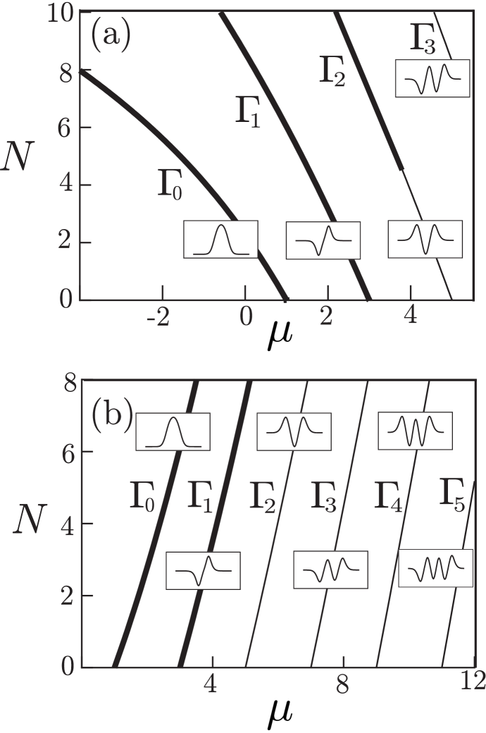
Figure 1: $N(\mu)$ curves for the NHO model, based on Eq. (38), with (a) $\sigma_{0}=1$ and (b) $\sigma_{0}=-1$, which correspond, respectively, to the self-attractive and repulsive signs of the nonlinearity (as per Refs. [17, 37]). Bold (thin) segments correspond to stable (unstable) modes. Insets show schematic profiles $u_{n}(x)$ of modes from each family.

Analysis of the eigenvalues of the matrix $\tilde{M}_{n}$ with $P(x)\equiv 1$ or $P(x)\equiv-1$ [37] shows that LMs corresponding to $\Gamma_{0}$ and $\Gamma_{1}$ are stable in the small-amplitude limit for both signs of the nonlinearity, $\sigma_{0}=1$ and $\sigma_{0}=-1$ [36, 46]. Numerical results indicate that these modes remain stable for moderate and large amplitudes as well. The small-amplitude LMs belonging to the branch $\Gamma_{2}$ are unstable. For $\sigma_{0}=1$ (self-attraction), the instability of the branch $\Gamma_{2}$ persists for $\mu^{\ast}<\mu<5$ where $\mu^{\ast}\approx 3.83$. At $\mu<\mu^{\ast}$ these modes was reported to be stable [46]. For $\sigma_{0}=-1$ (self-repulsion), the branch $\Gamma_{2}$ are unstable in the whole interval of $\mu$ covered in Fig. 1 (however, it may become stable at still larger values of $N,$ not shown in Fig. 1 [34]). The small-amplitude modes for the branches $\Gamma_{n}$ with $n=3,4,\ldots$ are also unstable in both cases of $\sigma_{0}=\pm 1$.

4.1.2 The dc-ac case: an oscillating pseudopotential

Let us now consider the combination of the HO trapping potential with the pseudopotential which contains the periodic component, i.e., $P_{1}\neq 0$ in Eq. (37). In this case, a general picture of LM branches can be obtained by means of a numerical shooting algorithm, which is presented in detail in Ref. [46]. A representative example of the respective $N(\mu)$ curves with $\sigma_{0}=1$ (average self-attraction), $P_{1}=2$ (which implies that the sign of the local nonlinearity periodically flips) and $\Omega=8$ is displayed in Fig. 2, where one immediately observes that, apart from the branches $\Gamma_{n}$ originating from their linear counterparts, numerous branches of LMs without linear counterparts exist too. Thus, the presence of the ac component in the pseudopotential essentially enriches the diversity of available solutions. However, no branch without a linear counterpart is stable (in fact, the only stable solutions in Fig. 2 corresponds to the ground-state branch, $\Gamma_{0}$).

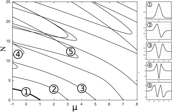
Figure 2: The dc-ac case. The main panel: $N(\mu)$ dependences, as obtained from Eq. (37) with $\sigma_{0}=1$, $P_{1}=2$, and $\Omega=8$. Thin and bold lines show unstable and stable LM families, the sole stable one being the lowest branch $\Gamma_{0}$. Insets (1)-(3) are representative profiles $u(x)$ of nonlinear modes originating their linear counterparts, for branches $\Gamma_{0}$, $\Gamma_{1}$, $\Gamma_{2}$ (labeled by the same numbers $1,2,3$), while insets (4) and (5) show profiles of modes belonging to some branches without linear counterparts, which are also labeled $4$ and $5$.

In the limit of the rapidly oscillation ac component, $\Omega\rightarrow\infty$, LMs may be approximated by the nonlinear HO modes. The asymptotic formula can be obtained by means of averaging with respect to the fast oscillations (see, e.g., Ref. [47]):

$$u(x)=u^{(0)}(x)+\frac{1}{\Omega^{2}}\left[u^{(1)}(x)+P_{1}(u^{(0)}(x))^{3}\cos\left(\Omega x\right)\right]+o\left(\frac{1}{\Omega^{2}}\right),\quad\Omega\rightarrow\infty.$$ (39)

Here $u^{(0)}(x)$ is a solution of nonlinear HO model corresponding to Eq. (38), and $u^{(1)}(x)$ is a localized solution of the linear equation

$$\frac{d^{2}u}{dx^{2}}+\left\{\mu-x^{2}+3\sigma_{0}\left[u^{(0)}(x)\right]^{2}\right\}u=-\frac{3}{2}P_{1}^{2}\left[u^{(0)}(x)\right]^{5}.$$ (40)

We stress that asymptotic relation (39) is valid for nonlinear modes of arbitrary amplitudes (i.e., not only in the small-amplitude limit), provided that $\Omega^{2}$ is large enough.

Figure 3 shows the branches $\Gamma_{0}$, $\Gamma_{1}$ and $\Gamma_{2}$ for two different spatial frequencies of the periodic pseudopotential, $\Omega=8$ and $\Omega=12$. According to the asymptotic prediction (39), they approach the corresponding branches of the nonlinear HO equation as $\Omega$ grows. Additionally, Eq. (39) implies that (in)stability of a LM under the action of the rapidly oscillating pseudopotential is determined by the (in)stability of its counterpart in the nonlinear HO model. Indeed, the presence of eigenvalues with nonzero real parts in the perturbative spectrum of an nonlinear HO state implies the existence of such eigenvalues in the spectrum of LM if $\Omega$ is large enough. We also conjecture that the stability of a nonlinear HO mode implies the stability of its LM counterpart for sufficiently large $\Omega$. For example, the segment of the branch $\Gamma_{1}$ shown in Fig. 2 is completely unstable for $\Omega=8$, but its stability restores for $\Omega=12$, which agrees with the nonlinear HO limit, where this branch is entirely stable. For the branch $\Gamma_{2}$ the situation is more complex. Small-amplitude modes belonging to $\Gamma_{2}$ are unstable for $\Omega=8$, but become stable for $\Omega=12$. However, Eq. (39) implies that the further increase of $\Omega$ will necessarily lead to the destabilization of these modes, because in the nonlinear HO limit the small-amplitude modes belonging to $\Gamma_{2}$ are unstable. The possibility to manage the stability of small-amplitude nonlinear LMs by tuning the frequency of the ac component of the pseudopotential has been recently reported in Ref. [22].

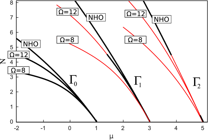
Figure 3: The dc-ac case. $N(\mu)$ curves for Eq. (37) with $\sigma_{0}=1$, $P_{1}=2$, and $\Omega=8$ or $\Omega=12$. Only branches $\Gamma_{0,1,2}$ are shown. For comparison, the corresponding dependencies for NHO equation (38) with $\sigma_{0}=1$ [identical to those in Fig. 1(a)] are shown too. Bold black lines (and thin red lines) correspond to stable (unstable) nonlinear modes.

To check the predictions of the linear-stability analysis, we have performed simulations of the evolution of LMs in the framework of the time-dependent GPE (34), using an implicit finite-difference scheme [48] with adsorbing boundary conditions. In the simulations, solutions which are predicted to be linearly stable keep their shape indefinitely long [see Fig.  4 (1a,b)], whereas the nonlinear modes which are predicted to be unstable typically transform into a pulsating object localized over one period of the lattice pseudopotential, see Figs. 4 (2a,b).

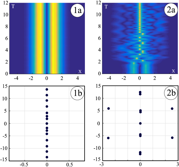
Figure 4: The dc-ac case, $P(x)=1+2\cos 16x$. (1a): The evolution of a stable LM with $\mu=0$, belonging to branch $\Gamma_{1}$. (1b): The spectrum of the eigenvalue problem (11) associated with this LM. (2a): The evolution of an unstable LM with $\mu=-3$, belonging to branch $\Gamma_{1}$. (2b) The corresponding spectrum of the eigenvalue problem (11).

4.2 Nonlinear pseudopotential with zero mean (the ac case)

According to the results of the previous subsection, the effect of a rapidly oscillating ac component of the pseudopotential, in the presence of the dc component, may be approximated using the standard nonlinear HO model with the uniform nonlinearity. However, the situation becomes essentially different in the absence of the dc component. We address the latter situation using Eq. (36). The corresponding nonlinear modes can be found from the equation

$$\frac{d^{2}u}{dx^{2}}+(\mu-x^{2})u+\sigma_{1}\cos(\Omega x)u^{3}=0.$$ (41)

The so obtained $N(\mu)$ curves are shown in the main panel of Fig. 5. Here we again observe the branches $\Gamma_{n}$ bifurcating from the linear limit [Fig. 5, insets (1) and (2)] and various families without linear counterparts [Fig. 5, insets (3-4)]. The branches $\Gamma_{n}$ feature stable and unstable segments, all LMs without linear counterpart being unstable, as above.

4.2.1 Shapes of solutions with linear counterparts

In the limit $N\ll 1$, weakly nonlinear LMs belonging to branches $\Gamma_{n}$, $n=0,1,\ldots$, are produced by Eqs. (20) where $\Delta_{n}$ is given by Eq. (21), with $P(x)=\sigma_{1}\cos\left(\Omega x\right)$. The numerically found values of $\Delta_{n}$, $n=0,1,2$, for $\sigma_{1}=1$ and several different values of $\Omega$ are presented in Table 1.

$\Omega$	0	2	8	18
$n=0$	$\quad 3.9894\cdot 10^{-1}$	$2.4197\cdot 10^{-1}$	$1.3383\cdot 10^{-4}$	$1\cdot 10^{-18}$
$n=1$	$2.9921\cdot 10^{-1}$	$-1.2100\cdot 10^{-1}$	$5.4536\cdot 10^{-3}$	$2\cdot 10^{-15}$
$n=2$	$2.5557\cdot 10^{-1}$	$-1.3611\cdot 10^{-1}$	$2.1097\cdot 10^{-2}$	$5\cdot 10^{-13}$

Table 1: The ac case. The values of $\Delta_{n}$, $n=0,1,2$, calculated as per Eq. (21), for $P(x)=\cos\left(\Omega x\right)$, $\Omega=0,2,8,18$. They determine the perturbative shift of chemical potential of weakly nonlinear LMs, pursuant to Eq. (20).

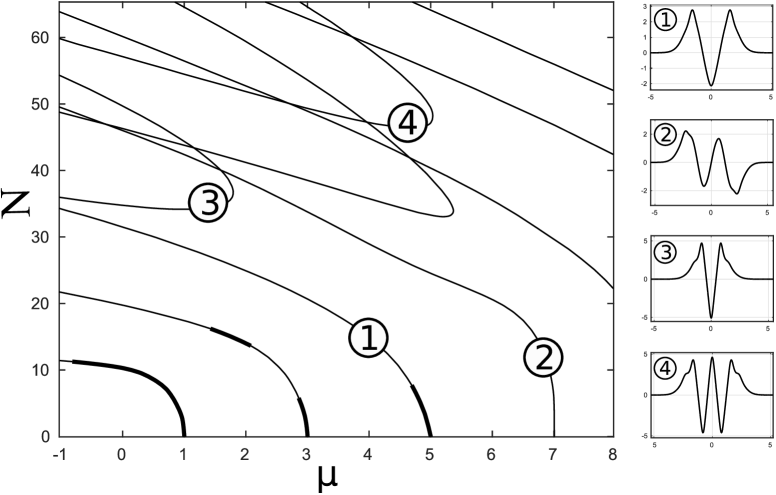
Figure 5: The ac case. The main panel: $N(\mu)$ curves for $P(x)=\cos(8x)$, thin and bold lines showing unstable and stable LM families, respectively. (1) and (2) label branches $\Gamma_{2}$, $\Gamma_{3}$, while (3) and (4) pertain to ones without linear counterparts. Profiles of the LMs for branches (1)-(4) are depicted in separate panels.

To find the asymptotic form of $\Delta_{n}$ for $\Omega\rightarrow\infty$, we note that, for an arbitrary polynomial $Q_{2m}(x)=a_{2m}x^{2m}+a_{2m-1}x^{2m-1}+\ldots+a_{0}$ of degree $2m$, the following asymptotic relation holds:

$$\int_{-\infty}^{+\infty}Q_{2m}(x)e^{-2x^{2}}\cos\left(\Omega x\right)~{}dx\approx(-1)^{m}\frac{a_{2m}\sqrt{2\pi}\Omega^{2m}}{2^{4m+1}}e^{-\Omega^{2}/8},\quad\Omega\rightarrow\infty.$$ (42)

Since the coefficient in front of the highest-power term in the Hermite polynomial $H_{n}(x)$ is $2^{n}$, Eq. (42) with $Q_{2m}(x)$ substituted by $H_{n}(x)$ yields

$$\Delta_{n}\approx\frac{\sqrt{2}\Omega^{4n}}{2^{6n+1}\cdot(n!)^{2}\sqrt{\pi}}e^{-\Omega^{2}/8},\quad\Omega\rightarrow\infty.$$ (43)

Therefore, for sufficiently large $\Omega$, $\Delta_{n}$ are all positive and decay exponentially, which agrees with the data in Table 1.

As has been shown above [see Eq. (39)], in the model with rapidly oscillating pseudopotential and nonzero dc term, the shapes of LMs may be approximated by the corresponding solutions of the nonlinear HO equation. However, the asymptotic behavior of LMs in the limit of $\Omega\rightarrow\infty$ becomes essentially different for the pseudopotential without the dc term. Indeed, nonlinear mode $u(x)$ belonging to the branch $\Gamma_{n}$ which satisfies Eq. (41), may be looked for as

$$u(x)=W(x)+R(x)\cos\left(\Omega x\right)+\mathrm{higher}~{}\mathrm{order}~{}\mathrm{terms},$$ (44)

where $W(x)$ and $R(x)$ are slowly varying functions in comparison with $\cos\left(\Omega x\right)$. Then one arrives at the balance relation between the dominating terms:

$$R(x)\Omega^{2}=\sigma_{1}W^{3}(x).$$ (45)

In the next order of $1/\Omega$, one arrives at the equation for $W(x)$,

$$\frac{d^{2}W}{dx^{2}}+(\mu-x^{2})W+\frac{3}{2\Omega^{2}}W^{5}=0.$$ (46)

Introducing a rescaled function, $U(x)=W(x)/\sqrt{\Omega}$, one obtains the following approximation:

$$u(x)=\sqrt{\Omega}U(x)+\frac{\sigma_{1}}{\sqrt{\Omega}}U^{3}(x)\cos\Omega x+o\left(\frac{1}{\sqrt{\Omega}}\right),$$ (47)

where $U(x)$ is a localized solution of the equation

$$\frac{d^{2}U}{dx^{2}}+(\mu-x^{2})U+\frac{3}{2}U^{5}=0.$$ (48)

While Eq. (48) does not admit any simple analytical solution, its localized modes can be computed numerically and used in Eq. (47) to approximate nonlinear modes in the rapidly oscillating pseudopotential (compare grey and red lines in Fig. 6). To obtain the asymptotic expression for the shapes of nonlinear modes in explicit analytical form, we define $\Delta\mu=\tilde{\mu}_{n}-\mu$ and rewrite Eq. (48) as

$$\frac{d^{2}U}{dx^{2}}+(\tilde{\mu}_{n}-x^{2})U=-\frac{3}{2}U^{5}+\Delta\mu U.$$ (49)

If $\Delta\mu$ is not large, one may assume that $U(x)\approx U_{0}H_{n}(x)e^{-x^{2}/2}$, where $U_{0}$ is some constant which can be found from the requirement for right-hand side of (49) to be orthogonal to the kernel of the operator in the left-hand side:

$$\int_{-\infty}^{+\infty}\left(-\frac{3}{2}U^{5}(x)+\Delta\mu U(x)\right)H_{n}(x)e^{-x^{2}/2}~{}dx=0,$$ (50)

which leads to

$$U_{0}=\left(\frac{2{\mathcal{H}}_{n}^{(2)}\Delta\mu}{3{\mathcal{H}}_{n}^{(6)}}\right)^{\frac{1}{4}},$$ (51)

$${\mathcal{H}}_{n}^{(2)}\equiv\int_{-\infty}^{+\infty}H_{n}^{2}(x)e^{-x^{2}}~{}dx,\quad{\mathcal{H}}_{n}^{(6)}\equiv\int_{-\infty}^{+\infty}H_{n}^{6}(x)e^{-3x^{2}}~{}dx.$$ (52)

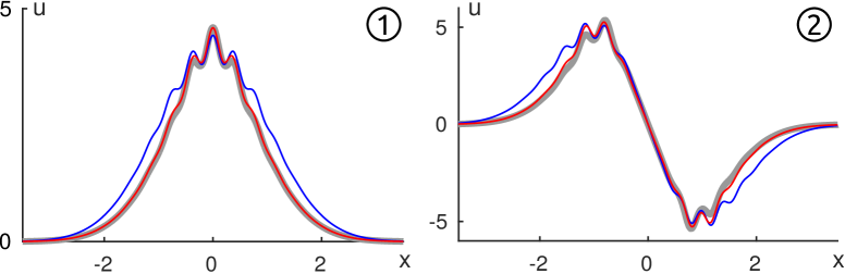
Figure 6: The ac case. Profiles of LMs, for $P(x)=\cos\left(16x\right)$. (1) Branch $\Gamma_{0}$, $\mu=0$ ($\Delta\mu=1$). (2) Branch $\Gamma_{1}$, $\mu=1$ ($\Delta\mu=2$). Gray line: the numerical solution, red line: approximation (47), with $U(x)$ obtained by numerical solution of Eq. (48). Blue line: approximation (53).

Combining the obtained results with Eq. (47), one finally gets

$$u(x)\approx\left(\frac{2{\mathcal{H}}_{n}^{(2)}\Delta\mu}{3{\mathcal{H}}_{n}^{(6)}}\right)^{1/4}\sqrt{\Omega}H_{n}(x)e^{-x^{2}/2}+\left(\frac{2{\mathcal{H}}_{n}^{(2)}\Delta\mu}{3{\mathcal{H}}_{n}^{(6)}}\right)^{3/4}\frac{\sigma_{1}}{\sqrt{\Omega}}H_{n}^{3}(x)e^{-3x^{2}/2}\cos\left(\Omega x\right).$$ (53)

For the lowest branch $\Gamma_{0}$ Eq. (53) yields

$$u(x)\approx\left(\frac{2\Delta\mu}{\sqrt{3}}\right)^{1/4}\sqrt{\Omega}e^{-x^{2}/2}+\left(\frac{2\Delta\mu}{\sqrt{3}}\right)^{3/4}\frac{\sigma_{1}}{\sqrt{\Omega}}e^{-3x^{2}/2}\cos\left(\Omega x\right).$$ (54)

For the next branch, $\Gamma_{1}$, one obtains

$$u(x)\approx\left(\frac{216\Delta\mu}{15\sqrt{3}}\right)^{1/4}\sqrt{\Omega}xe^{-x^{2}/2}+\left(\frac{216\Delta\mu}{15\sqrt{3}}\right)^{3/4}\frac{\sigma_{1}}{\sqrt{\Omega}}x^{3}e^{-3x^{2}/2}\cos\left(\Omega x\right).$$ (55)

The comparison between the numerical solution and approximations (47) and (53) is illustrated by the Fig. 6, for $\Omega=16$. The figure shows that approximation (47) describes the numerical solution very well. Approximation (53) is good too, even if $\Delta\mu$ is not small (compare grey and blue lines in Fig. 6, where $\Delta\mu=1$ and $2$ in the left and right panels, respectively).

4.2.2 Stability of localized modes

In the small-amplitude limit, the stability of LMs is determined by the eigenvalues of matrix $\tilde{M}_{n}$, see Sect. 3. Using Maple, one can compute these eigenvalues with any necessary accuracy. The results for two modulation frequencies ($\Omega=8$ and $16$) are summarized in Tables 2-3. In these tables, $n$ is the index of the branch $\Gamma_{n}$ (for instance, $n=2$ means that the branch $\Gamma_{2}$, which starts from $\tilde{\mu}_{2}=2\cdot 2+1=5$, is under consideration), while $k$, running from $0$ to $n-1$, enumerates double eigenvalues $\tilde{\Lambda}_{k}=4(n-k)^{2}$. Each cell with $n\geq k$ contains either letter “C” or two real numbers. These numbers are the real eigenvalues $\gamma_{1,2}$ of the matrix $\tilde{M}_{n}$, whereas “C” means that both eigenvalues of $\tilde{M}_{n}$ are complex. For $n<k$ the double eigenvalues do not exist (dashes at the corresponding positions in the table).

		$n=1$		$n=2$		$n=3$		$n=4$		$n=5$
$k=0$		$\begin{array}[]{c}0.132\\ -0.028\end{array}$		$\begin{array}[]{c}-0.012\\ 0.203\end{array}$		C		$\begin{array}[]{c}0.424\\ -0.828\end{array}$		$\begin{array}[]{c}-0.845\\ -0.660\end{array}$
$k=1$		–		$\begin{array}[]{c}-0.176\\ 0.159\end{array}$		$\begin{array}[]{c}0.432\\ -0.190\end{array}$		$\begin{array}[]{c}-0.486\\ 0.048\end{array}$		$\begin{array}[]{c}0.356\\ 0.944\end{array}$
$k=2$		–		–		$\begin{array}[]{c}-0.068\\ -0.132\end{array}$		$\begin{array}[]{c}-0.206\\ 0.196\end{array}$		$\begin{array}[]{c}0.531\\ -0.600\end{array}$
$k=3$		–		–		–		C		$\begin{array}[]{c}0.166\\ -0.122\end{array}$
$k=4$		–		–		–		–		C

Table 2: Eigenvalues of matrix $\tilde{M}$, in the case of $P(x)=\cos\left(8x\right)$. Here $n$ is the index of branch $\Gamma_{n}$, and $k$ enumerates double eigenvalues $\tilde{\Lambda}_{k}=4(n-k)^{2}$. Each cell with $n>k$ contains either letter “C” or two real numbers. These numbers are real eigenvalues $\gamma_{1,2}$ of matrix $\tilde{M}_{n}$, whereas letter “C” means that eigenvalues of $\tilde{M}_{n}$ are complex.

		$n=1$		$n=2$		$n=3$		$n=4$		$n=5$
$k=0$		$\begin{array}[]{c}-2.0\cdot 10^{-11}\\ 5.7\cdot 10^{-10}\end{array}$		$\begin{array}[]{c}-7.6\cdot 10^{-9}\\ -9.2\cdot 10^{-7}\end{array}$		$\begin{array}[]{c}-8.7\cdot 10^{-7}\\ 2.2\cdot 10^{-4}\end{array}$		$\begin{array}[]{c}-4.0\cdot 10^{-5}\\ -1.2\cdot 10^{-2}\end{array}$		$\begin{array}[]{c}-9.5\cdot 10^{-4}\\ 1.5\cdot 10^{-1}\end{array}$
$k=1$		–		$\begin{array}[]{c}-4.2\cdot 10^{-9}\\ 7.3\cdot 10^{-8}\end{array}$		$\begin{array}[]{c}-5.8\cdot 10^{-7}\\ -3.6\cdot 10^{-5}\end{array}$		$\begin{array}[]{c}-3.0\cdot 10^{-5}\\ 3.3\cdot 10^{-3}\end{array}$		$\begin{array}[]{c}-7.6\cdot 10^{-4}\\ -6.8\cdot 10^{-2}\end{array}$
$k=2$		–		–		$\begin{array}[]{c}-3.4\cdot 10^{-7}\\ 3.9\cdot 10^{-6}\end{array}$		$\begin{array}[]{c}-2.0\cdot 10^{-5}\\ -6.8\cdot 10^{-4}\end{array}$		$\begin{array}[]{c}-5.7\cdot 10^{-4}\\ 2.6\cdot 10^{-2}\end{array}$
$k=3$		–		–		–		$\begin{array}[]{c}-1.3\cdot 10^{-5}\\ 1.0\cdot 10^{-4}\end{array}$		$\begin{array}[]{c}-3.6\cdot 10^{-4}\\ -6.8\cdot 10^{-3}\end{array}$
$k=4$		–		–		–		–		$\begin{array}[]{c}-2.7\cdot 10^{-4}\\ 1.5\cdot 10^{-3}\end{array}$

Table 3: Eigenvalues of matrix $\tilde{M}_{n}$ for $P(x)=\cos\left(16x\right)$. The notation is the same as in Table 2.

To be specific, let us describe in detail the branch $\Gamma_{2}$ in the case of $P(x)=\cos\left(8x\right)$ (i.e., $n=2$ in Table 2). In this case, there are two double eigenvalues in the spectrum, $\tilde{\Lambda}_{0}=16$ and $\tilde{\Lambda}_{1}=4$. According to Table 2 and Eq. (28), they split as

$$\Lambda_{0}^{(1)}=16-0.012\cdot\varepsilon^{2}+\ldots,\quad\Lambda_{0}^{(2)}=16+0.203\cdot\varepsilon^{2}\ldots~{}$$ (56)

and

$$\Lambda_{1}^{(1)}=4-0.176\cdot\varepsilon^{2}+\ldots,\quad\Lambda_{1}^{(2)}=4+0.159\cdot\varepsilon^{2}\ldots~{},$$ (57)

hence the small-amplitude nonlinear LMs belonging to the branch $\Gamma_{2}$ are stable in this case. The situation is different for $\Gamma_{3,4,5}$, since for each of these branches the bifurcation of a complex-conjugate pair occurs: for $n=3$ the eigenvalue $\tilde{\Lambda}_{0}=36$ splits into complex eigenvalues,while for $n=4$ and $n=5$ this takes place for $\tilde{\Lambda}_{2}=4$. Therefore, for $\Omega=8$ the small-amplitude LMs are stable in the branches $\Gamma_{0}$, $\Gamma_{1}$ and $\Gamma_{2}$, but unstable in $\Gamma_{3}$, $\Gamma_{4}$ and $\Gamma_{5}$. Table 3 is produced for $\Omega=18$, implying that the small-amplitude LMs are stable for all the branches, $\Gamma_{0,\ldots,5}$.

To explain the different stability of small-amplitude LMs with different spatial frequencies $\Omega$, we consider the behavior of the eigenvalues of $\tilde{M}_{n}$ at $\Omega\rightarrow\infty$. Using explicit results given by Eqs. (29)–(31) and asymptotic relation (42), we obtain

$$\langle M_{n}\tilde{u}_{k},\tilde{u}_{k}\rangle \sim-\frac{2\sqrt{2}(n-k)\Omega^{4n}}{2^{6n}\cdot(n!)^{2}\sqrt{\pi}}e^{-\Omega^{2}/8},$$ (58)

$$\langle M_{n}\tilde{u}_{k},\tilde{u}_{2n-k}\rangle =-\langle M_{n}\tilde{u}_{2n-k},\tilde{u}_{k}\rangle\sim\frac{2\sqrt{2}(n-k)\Omega^{4n}}{2^{6n}n!\sqrt{k!(2n-k)!}\sqrt{\pi}}e^{-\Omega^{2}/8},$$ (59)

$$\langle M_{n}\tilde{u}_{2n-k},\tilde{u}_{2n-k}\rangle \sim-\frac{4\sqrt{2}(n-k)\Omega^{2(3n-k)}}{\sqrt{\pi}2^{3(3n-k)}n!(2n-k)!}e^{-\Omega^{2}/8}.$$ (60)

These relations imply that

$$\tilde{M}_{n}=\left(\begin{array}[]{cc}O(\Omega^{4n}e^{-\Omega^{2}/8})&O(\Omega^{4n}e^{-\Omega^{2}/8})\\[5.69054pt] O(\Omega^{4n}e^{-\Omega^{2}/8})&O(\Omega^{2(3n-k)}e^{-\Omega^{2}/8})\end{array}\right),\quad\Omega\rightarrow\infty$$ (61)

All elements of the matrix $\tilde{M}_{n}$ are of the same order, except for the one in the right lower corner which is of greater order due to $n>k$. This means that, for $\Omega$ large enough, eigenvalues of $\tilde{M}_{n}$ are real, hence the nonlinear LMs from branch $\Gamma_{n}$ for arbitrary $n$ are stable, at least in the small-amplitude limit. This explains the difference between the results displayed in Tables 2 and 3: the increase of the spatial frequency from $\Omega=8$ to $\Omega=16$ results in stabilization of some small-amplitude LMs which were originally unstable.

Rigorously speaking, the results for the linear stability of the small-amplitude LMs are asymptotic, and, while moving along a branch $\Gamma_{n}$ to the region of moderate or large amplitudes, the nonlinear LMs may change the stability. To illustrate the persistence of the asymptotic predictions for the (in)stability of the nonlinear LMs, in Fig. 7 we plot numerically obtained dependencies of eigenvalues $\lambda$ on $\mu$ for branches $\Gamma_{0,1,2,3}$ in the case of $P(x)=\cos\left(16x\right)$. Each shown branch is stable near the point of its emergence, losing stability at some threshold value of $\mu$ (which is different for different branches).

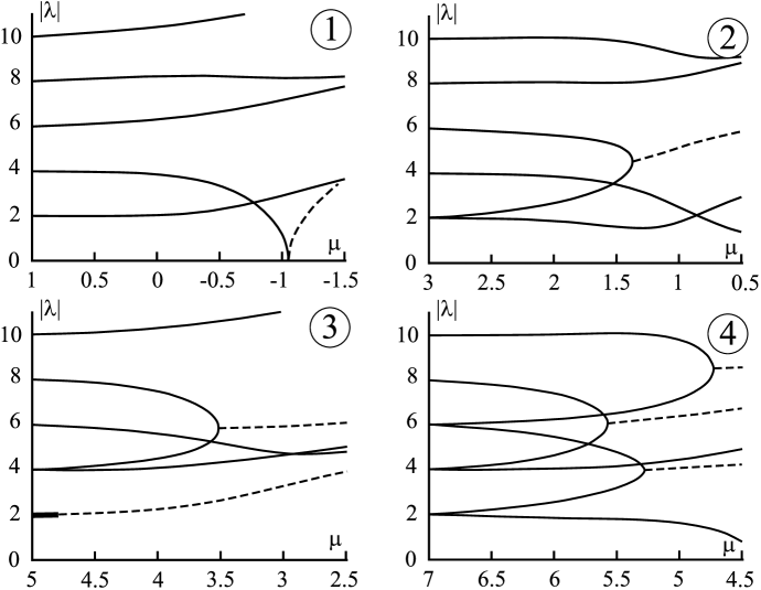
Figure 7: The evolution of eigenvalues of (11) as $\mu$ varies, for $P(x)=\cos\left(16x\right)$. Only eigenvalues with $\mathrm{Im}~{}\lambda\geq 0$ are shown. Solid line: pure imaginary eigenvalues corresponding to stable LMs; dashed line: eigenvalues with a nonzero real part. (1) Branch $\Gamma_{0}$. No double eigenvalues exist at $\mu=1$, all the eigenvalues being pure imaginary and simple, until the collision at $\mu\approx-1.049$. After the collision a pair of real eigenvalues emerges. (2) Branch $\Gamma_{1}$. At $\mu=3$ there exists one double eigenvalue, $\lambda=2i$. According to the prediction of the asymptotic analysis, it splits into a pair of pure imaginary simple eigenvalues. The collision of eigenvalues occurs at $\mu\approx 1.372$, and a pair of eigenvalues with nonzero real parts emerges. (3) Branch $\Gamma_{2}$. At $\mu=5$, there exists two pairs of double eigenvalues, $\lambda=2i$ and $\lambda=4i$. Both of them split into pairs of pure imaginary eigenvalues. The former pair collides again at $\mu\approx 4.801$ and transforms into a pair of complex eigenvalues with nonzero real parts. At $\mu\approx 3.519$ , another collision of eigenvalues occurs. (4) Branch $\Gamma_{3}$. At $\mu=7$, there exist three pairs of double eigenvalues. The first collision of pure imaginary eigenvalues takes place at $\mu\approx 5.571$, then two more collisions occur. They all result in eigenvalues with nonzero real parts.

Numerically generated $N(\mu)$ curves for $\Omega=8$, $\Omega=12$, and $\Omega=16$ are plotted in Fig. 8. It follows from these plots that the branch $\Gamma_{0}$ is the “most stable” one for all the three values of $\Omega$. One also notices that, for the greatest value of $\Omega$ (i.e., $\Omega=16$) there exists a “stability window” in a vicinity of the bifurcations for all branches $\Gamma_{0,1,2,3}$, in agreement with the asymptotic results presented above.

Numerical study of the temporal evolution of LMs in the framework of time-dependent GPE (36) confirms the predictions of the linear-stability analysis, see Fig. 9. As an example of a distinctive pattern of dynamical behavior of unstable modes, in Fig. 9 (2a) we display the transformation of an unstable solution into a pulsating object localized over one period of the lattice pseudopotential.

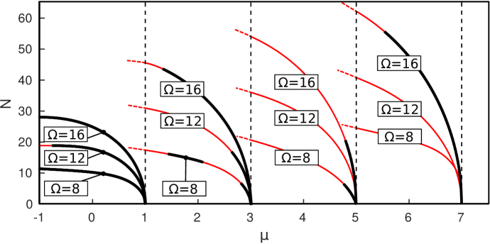
Figure 8: The ac case. $N(\mu)$ curves for $P(x)=\cos\left(\Omega x\right)$, $\Omega=8,12,16$. Branches $\Gamma_{0,1,2,3}$ are presented. Black bold (red thin) lines correspond to stable (unstable) LMs.

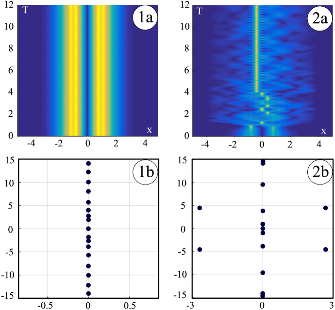
Figure 9: The ac case, $P(x)=\cos\left(16x\right)$. (1a): The evolution of a stable nonlinear mode belonging to branch $\Gamma_{1}$, with $\mu=2$. (1b): the spectrum of eigenvalues $\lambda$ produced by numerical solution of Eq. (11) associated with this mode. (2a): The evolution of an unstable mode belonging to branch $\Gamma_{1}$, with $\mu=0$; (2b) the corresponding spectrum.

5 Conclusion

In the paper, we have systematically studied nonlinear localized modes (LMs) of the one-dimensional Gross-Pitaevskii/nonlinear Schrödinger equation with the harmonic-oscillator (HO) trapping potential $V(x)$ and nonlinear lattice pseudopotential $P(x)$, which is an periodic function oscillating with spatial frequency $\Omega$. This equation describes a cigar-shaped cloud of BEC confined by the magnetic trap and manipulated by the optically-induced Feshbach resonance with the periodically modulated local strength. The model is characterized by the interplay between two spatial scales: the characteristic size of the HO trap and the period of the nonlinear lattice pseudopotential. This factor essentially enriches the variety of nonlinear modes in this model, in comparison with the well-studied case of the spatially uniform nonlinearity. We have obtained analytical results of the shape of nonlinear LMs and on their stability, in the limits of small-amplitude solutions and rapidly oscillating pseudopotential. The validity and persistence of the asymptotic predictions has been corroborated by systematically presented numerical findings.

To conclude the paper, it is relevant, once again, to highlight its main results. It was found that there exist two types of branches of LMs, viz., ones with and without linear counterpart. This is especially interesting in view of the fact that no modes without linear counterpart exists in the model with the uniform nonlinearity. However, all these “exotic” nonlinear modes, disconnected from the linear limit, are unstable. As concerns nonlinear LMs bifurcating from eigenstates of the underlying linear problem, their properties are essentially different depending on the presence of the dc term (nonzero mean value) in the periodic pseudopotential. If the mean is nonzero, then properties of nonlinear modes in a rapidly oscillating pseudopotential may be approximated using solutions for the standard HO model with constant nonlinearity. However, the reduction to the standard model with constant nonlinearity does not work for the system in a rapidly oscillating pseudopotential without the dc term. Most interestingly, in this case we have found that the rapidly oscillating pseudopotential can stabilize small-amplitude LMs belonging to higher families (excited states, which are unstable in the model including the dc term). Specifically, for any given branch with index $n$, there exists a threshold value of the spatial frequency, $\Omega_{n}$, such that the small-amplitude solutions belonging to this branch are stable for $\Omega>\Omega_{n}$.

As a continuation of this work, it may be interesting to extend the analysis to the case of the interplay between the spatially periodic pseudopotential and the expulsive (anti-HO) potential. A more challenging possibility is to consider a two-dimensional model featuring the combination of an isotropic HO trapping potential and two-dimensional lattice quasipotential.

References

References

- [1] Anderson MH, Ensher JR, Matthews MR, Wieman CE, and Cornell EA. Observation of Bose-Einstein condensation in a dilute atomic vapor. Science 1995;269:198-201.
- [2] Davis KB, Mewes M-O., Andrews MR, van Druten NJ, Durfee DS, Kurn DM, Ketterle W. Bose-Einstein condensation in a gas of sodium atoms. Phys Rev Lett 1995;75:3969.
- [3] Bradley CC, Sackett CA, Tollett JJ, Hulet RG. Evidence of Bose-Einstein condensation in an atomic gas with attractive interactions. Phys Rev Lett 1995;75:1687.
- [4] Bagnato VS, Frantzeskakis DJ, Kevrekidis PG, Malomed BA, Mihalache D. Bose-Einstein condensation: Twenty years after. Rom Rep Phys 2015;67:5-50.
- [5] Inouye S, Andrews MR, Stenger J, Miesner HJ, Stamper-Kurn DM, Ketterle W. Observation of Feshbach resonances in a Bose-Einstein condensate. Nature (London) 1998;392:151.
- [6] Theis M, Thalhammer G, Winkler K, Hellwig M, Ruff G, Grimm R, Denschlag JH. Tuning the scattering length with an optically induced Feshbach resonance. Phys Rev Lett 2004;93:123001.
- [7] Kohler T, Goral K, and Julienne PS. Production of cold molecules via magnetically tunable Feshbach resonances. Rev Mod Phys 2006;78:1311.
- [8] Ghanbari S, Kieu TD, Sidorov A, Hannaford P. Permanent magnetic lattices for ultracold atoms and quantum degenerate gases. J Phys B: At Mol Opt Phys 2006;39:847-860.
- [9] Yamazaki R, Taie S, Sugawa S, Takahashi Y. Submicron spatial modulation of an interatomic interaction in a Bose-Einstein condensate. Phys Rev Lett 2010;105:050405.
- [10] Clark LW, Ha L-C, Xu C-Y, Chin C. Quantum dynamics with spatiotemporal control of interactions in a stable Bose-Einstein condensate. Phys Rev Lett 2015;115:155301.
- [11] Sakaguchi H, Malomed BA. Solitons in combined linear and nonlinear lattice potentials. Phys Rev A 2010;81:013624.
- [12] Pethick CJ, Smith H. Bose-Einstein Condensation in Dilute Gases: (Cambridge University Press: Cambridge; 2002).
- [13] Pitaevskii LP, Stringari A. Bose-Einstein Condensation: (Clarendon Press: Oxford; 2003).
- [14] Salasnich L, Parola A, and Reatto L. Effective wave equations for the dynamics of cigar-shaped and disk-shaped Bose condensates. Phys Rev A 2002;65:043614.
- [15] Muñoz Mateo A, Delgado V. Effective mean-field equations for cigar-shaped and disk-shaped Bose-Einstein condensates. Phys Rev A 2008;77:013617.
- [16] Harrison WA. Pseudopotentials in the Theory of Metals(Benjamin: New York; 1966).
- [17] Zezyulin DA, Alfimov GL, Konotop VV, Pérez-García VM. Control of nonlinear modes by scattering-length management in Bose-Einstein condensates. Phys Rev A 2007;76:013621.
- [18] Tsitoura F, Anastassi ZA, Marzuola JL, Kevrekidis PG, Frantzeskakis DJ. Dark solitons near potential and nonlinearity steps. Phys Rev A 2016;94:063612.
- [19] Rodrigues AS, Kevrekidis PG, Porter MA, Frantzeskakis DJ, Schmelcher P, Bishop AR. Matter-wave solitons with a periodic, piecewise-constant scattering length. Phys Rev A 2008;78:013611.
- [20] Wang C, Law KJH, Kevrekidis PG, Porter MA. Dark solitary waves in a class of collisionally inhomogeneous Bose-Einstein condensates. Phys Rev A 2013;87:023621.
- [21] Sakaguchi H, Malomed BA. Matter-wave solitons in nonlinear optical lattices. Phys Rev E 2005;72:046610.
- [22] Kevrekidis PG, Carretero-González R, Frantzeskakis DJ. Stability of single and multiple matter-wave dark solitons in collisionally inhomogeneous Bose Einstein condensates. Intern J Mod Phys B 2017;31:1742013.
- [23] Morsch O, Oberthaler M. Dynamics of Bose-Einstein condensates in optical lattices. Rev Mod Phys 2006;78:179-215.
- [24] Theocharis G, Schmelcher P, Kevrekidis PG, Frantzeskakis DJ. Matter-wave solitons of collisionally inhomogeneous condensates. Phys Rev A 2005;72:033614.
- [25] Hao R, Yang R, Li L, Zhou G. Solutions for the propagation of light in nonlinear optical media with spatially inhomogeneous nonlinearities. Opt Commun 2008;281:1256.
- [26] Dror N, Malomed B. A. Solitons and vortices in nonlinear potential wells. J Opt 2016;18:014003.
- [27] Kartashov YV, Malomed BA, Torner L. Solitons in nonlinear lattices. Rev Mod Phys 2011;83:247-306.
- [28] Borovkova OV, Kartashov YV, Torner L, Malomed BA. Bright solitons from defocusing nonlinearities. Phys Rev E 2011;84:035602(R).
- [29] Alfimov GL, Konotop VV, Salerno M. Matter solitons in Bose-Einstein condensates with optical lattices. Europhys Lett 2002;58:7-13.
- [30] Yang J. Nonlinear Waves in Integrable and Nonintegrable Systems (Society for Industrial and Applied Mathematics: Philadelphia; 2010).
- [31] D’Agosta R, Malomed BA, Presilla C. Stationary states of Bose–Einstein condensates in single- and multi-well trapping potentials. Laser Phys 2002;12:37.
- [32] D’Agosta R, Presilla C. States without a linear counterpart in Bose-Einstein condensates. Phys Rev A 2002;65:043609.
- [33] Zeng J, Malomed BA. Localized dark solitons and vortices in defocusing media with spatially inhomogeneous nonlinearity. Phys Rev E 2017;95:052214.
- [34] Coles MP, Pelinovsky DE, Kevrekidis P. G. Excited states in the large density limit: a variational approach. Nonlinearity 2010;23:1753-1770.
- [35] Pelinovsky DE, Frantzeskakis DJ, Kevrekidis P. G. Oscillations of dark solitons in trapped Bose-Einstein condensates. Phys Rev E 2005;72:016615.
- [36] Kevrekidis PG, Konotop VV, Rodrigues A, Frantzeskakis DJ. Dynamic generation of matter solitons from linear states via time-dependent scattering lengths. J Phys B: At Mol Opt Phys 2005;38:1173-1178.
- [37] Zezyulin DA, Alfimov GL, Konotop VV, Pérez-García VM. Stability of excited states of a Bose-Einstein condensate in an anharmonic trap. Phys Rev A 2008;78:013606.
- [38] Zezyulin DA, Konotop VV. Small-amplitude nonlinear modes under the combined effect of the parabolic potential, nonlocality and symmetry. Symmetry 2016;8:72.
- [39] Edwards M, Burnett K. Numerical solution of the nonlinear Schrödinger equation for small samples of trapped neutral atoms. Phys Rev A 1995;51:1382-1386.
- [40] Kunze M, Küpper T, Mezentsev VK, Shapiro EG, Turitsyn S. Nonlinear solitary waves with Gaussian tails. Physica D 1999;128:273–295.
- [41] Gammal A, Frederico T, Tomio L. Improved numerical approach for the time-independent Gross-Pitaevskii nonlinear Schrödinger equation. Phys Rev E 1999;60:2421.
- [42] Kivshar YuS, Alexander TJ, Turitsyn SK. Nonlinear modes of a macroscopic quantum oscillator. Phys Lett A 2001;278:225.
- [43] Carr LD, Kutz JN, and Reinhardt WP. Stability of stationary states in the cubic nonlinear Schrödinger equation: Applications to the Bose-Einstein condensate. Phys Rev E 2001;63:066604.
- [44] Yukalov VI, Yukalova EP, Bagnato VS. Nonlinear coherent modes of trapped Bose–Einstein condensates. Phys Rev A 2002;66:043602.
- [45] Konotop VV, Kevrekidis PG. Bohr-Sommerfeld quantization condition for the Gross-Pitaevskii equation. Phys Rev Lett 2003;91:230402.
- [46] Alfimov GL, Zezyulin DA. Nonlinear modes for the Gross-Pitaevskii equation — a demonstrative computation approach. Nonlinearity 2007;20:2075-2092.
- [47] Abdullaev FKh, Caputo JG, Kraenkel RA, Malomed BA. Controlling collapse in Bose-Einstein condensation by temporal modulation of the scattering length. Phys Rev A 2003;67: 013605.
- [48] Trofimov VA, Peskov NV. Comparison of finite-difference schemes for the Gross-Pitaevskii equation. Mathematical Modelling and Analysis 2009;14:109.