Investigating the relation between sunspots and umbral dots

Abstract

Umbral dots (UDs) are transient, bright features observed in the umbral region of a sunspot. We study the physical properties of UDs observed in sunspots of different sizes. The aim of our study is to relate the physical properties of umbral dots with the large-scale properties of sunspots. For this purpose, we analyze high-resolution G-band images of 42 sunspots observed by Hinode/SOT, located close to disk center. The images were corrected for instrumental stray-light and restored with the modeled PSF. An automated multi-level tracking algorithm was employed to identify the UDs located in selected G-band images. Furthermore, we employed HMI/SDO, limb-darkening corrected, full disk continuum images to estimate the sunspot phase and epoch for the selected sunspots. The number of UDs identified in different umbrae exhibits a linear relation with the umbral size. The observed filling factor ranges from 3% to 7% and increases with the mean umbral intensity. Moreover, the filling factor shows a decreasing trend with the umbral size. We also found that the observed mean and maximum intensities of UDs are correlated with the mean umbral intensity. However, we do not find any significant relationship between the mean (and maximum) intensity and effective diameter of umbral dots with the sunspot area, epoch, and decay rate. We suggest that this lack of relation could either be due to the distinct transition of spatial scales associated with overturning convection in the umbra or the shallow depth associated with umbral dots, or both the above.

1. Introduction

Umbral dots (UDs) are small, bright features observed in sunspot umbrae and pores. They cover only 3–10% of the umbral area and contribute 10–20% of its brightness (Sobotka et al., 1993; Watanabe et al., 2012). It has been suggested that umbral dots, light bridges etc. play a vital role in the energy balance of sunspots (Solanki, 2003). While the strong magnetic field in the umbra suppresses energy transport by convection, some form of energy transport must be required to explain the observed umbral brightness.

The nature of UDs has been described in a number of models. The cluster model of Parker (1979) proposes that the umbral magnetic field is gappy, allowing field-free plasma to transport heat. An UD would represent the tip of such a field-free intrusion. The monolithic flux tube model of Weiss (2002) considers a sunspot as a collection of uniform vertically thin columns, and UDs as a natural result of the overstable oscillatory convection, which is the preferred mode just below the photosphere. Simulations by Schüssler & Vögler (2006) show that UDs are the result of narrow, upflowing, convective plumes with adjacent downflows.

Based on their location, UDs are classified as central umbral dots (CUDs) and peripheral umbral dots (PUDs) (Grossmann-Doerth et al., 1986). CUDs appear in the inner regions of the umbra, whereas PUDs are located near the umbra-penumbra boundary. The size of UDs ranges from 180–300 km and their intensity ranges from about 0.2 to 0.7 times the quiet Sun (QS) intensity at visible wavelengths (Kitai et al., 2007; Sobotka et al., 1997; Louis et al., 2012a). The distribution of UDs in the umbra is not uniform, Sobotka et al. (1997) reported that larger, long-lived UDs are seen in regions of enhanced umbral background intensity. Watanabe et al. (2009) also reported that UDs are likely to appear in regions where the magnetic field is weaker and inclined, whereas they tend to disappear in locations where the field is stronger and vertical. In addition, their study shows that the lifetimes and sizes of UDs are almost constant, regardless of the magnetic field strength.

The physical properties of UDs have been extensively studied by several authors (Sobotka et al., 1997; Riethmüller et al., 2008; Hamedivafa, 2011; Watanabe et al., 2012; Louis et al., 2012a), but they are primarily confined to time sequence observations of single spots or spots in a single active region (AR). Watanabe (2014) investigated the spatial distribution of UDs in several sunspots using Hinode observations. The results showed that UDs became more clustered in the latter phase of sunspots. If UDs are driven by small-scale magnetoconvection in umbrae, then the sub-photospheric convective flows could influence the properties of UDs observed at the photosphere. The motivation of this article is to investigate if the macro-properties of sunspots, namely, area, umbral fill fraction, decay rate, and phase, have any bearing on the physical characteristics of UDs, specifically, intensity and size. To that extent, we combine observations from Hinode and and SDO/HMI to determine the properties of UDs and their host sunspots. The article is organized in the following manner. The observations and data analysis are described in Sect. 2. The algorithm used for the identification of UDs is discussed in Sect. 3. In Sect. 4, we present our results. The discussion and conclusions are presented in Sects. 5 and 6, respectively.

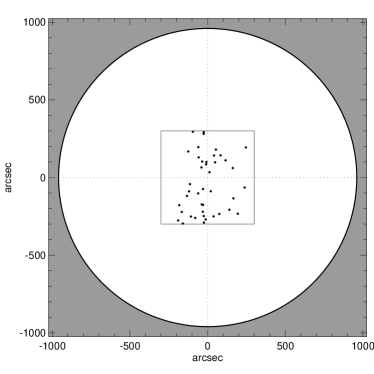
Figure 1.— The filled black circles depict the locations of the selected sunspots during Hinode observations on the artificial solar disk. The square represents the boundary of $\pm$5 arc-minute patch from the center of the solar disk.

2. Observations and data analysis

In order to study the physical properties of UDs in different sunspots, we employed high resolution G-band images acquired by the Broadband Filter Imager (BFI) of the Solar Optical Telescope (SOT; Tsuneta et al., 2008) on-board Hinode (Kosugi et al., 2007). The primary criterion for selecting the data was the proximity of sunspots to disc center to reduce the projection effects on the physical properties of UDs. Sunspots with heliocentric angles $\Theta\leqslant 25^{\circ}$ ($\mu\geqslant 0.9$) were chosen for the study. We carefully examined the G-band images of fully evolved sunspots with well developed penumbrae from Hinode observations that were acquired between 2013 January to 2014 December. During these two years, we found 42 sunspots that met our selection criterion. This period coincides with the maximum phase of solar cycle 24. Out of 42 sunspots, 18 were located in the northern hemisphere (Fig. 1). The details of the chosen sunspots are listed in Table 1. All selected Hinode images were corrected for dark current, flat-field, and bad-pixels using routines available in the Hinode SolarSoft package. The spatial sampling for a majority of the Hinode G-band images was 0$\farcs$22/pixel and 0$\farcs$11/pixel for 6 cases (Table 1).

Full-disk, limb-darkening-removed, continuum images from the Helioseismic and Magnetic Imager (HMI; Scherrer et al., 2012), on-board the Solar Dynamics Observatory (SDO; Pesnell et al., 2012), were employed to estimate the epoch, growth and decay-rate of the selected spots. The HMI images are 4096 $\times$ 4096 pixels in size, with a spatial sampling of around 0$\farcs$5/pixel and a time cadence of 6 hr.

Table 1Details of the ARs analyzed in the study. The effective umbral diameter (D_umb), and the normalized mean umbral intensity (I_umb) are given in the seventh, and eighth columns, respectively.

Spot	NOAA	Date	Time	xpos	ypos	Dumb	Iumb
No.	(AR $\#$)	(yy/mm/dd)	(UT)	(″)	(″)	(″)
1a	11692	2013/01/14	04:17:42	-87	211	12.7	0.16
2b	11765	2013/06/07	07:31:31	9	115	10.8	0.18
3b	11785	2013/07/07	21:21:30	-4	-260	16.3	0.11
4a	11809	2013/08/06	04:39:06	-3	59	8.8	0.17
5${}^{L}_{a}$	11861	2013/10/12	18:10:02	45	-234	16.6	0.12
6${}^{F}_{a}$	11861	2013/10/12	18:10:02	-55	-248	14.5	0.14
7a	11884	2013/11/07	17:32:10	-254	-274	19.5	0.09
8b	11890	2013/11/19	10:43:02	181	30	34.3	0.08
9${}^{L}_{a}$	11921	2013/12/15	17:41:38	-10	85	19.7	0.10
10${}^{F}_{a}$	11921	2013/12/15	17:41:38	-10	85	14.1	0.11
11b	11934	2013/12/26	10:28:02	58	-273	13.3	0.14
12${}^{L}_{a}$	11944	2014/01/07	08:44:58	-74	-65	40.0	0.09
13${}^{F}_{a}$	11944	2014/01/07	08:44:58	-180	-65	20.0	0.14
14a	11959	2014/01/23	10:48:31	-179	-214	18.8	0.14
15a	11960	2014/01/24	14:49:02	10	-332	16.2	0.12
16${}^{L}_{a}$	11967	2014/02/03	06:08:14	15	-147	37.9	0.10
17${}^{F}_{a}$	11967	2014/02/03	06:08:14	15	-147	30.6	0.11
18b	11974	2014/02/10	23:16:36	-210	-110	13.1	0.14
19a	11990	2014/03/03	01:45:03	50	-138	14.7	0.13
20a	11991	2014/03/03	06:55:01	-108	-251	9.1	0.16
21a	12002	2014/03/12	13:56:04	-254	-225	14.7	0.15
22a	12005	2014/03/18	00:35:00	-95	285	18.7	0.12
23a	12014	2014/03/26	11:29:57	166	-134	15.0	0.12
24a	12027	2014/04/06	04:16:59	-43	282	16.3	0.12
25a	12032	2014/04/13	16:14:59	-61	282	15.6	0.11
26${}^{L}_{a}$	12056	2014/05/11	18:50:57	-35	103	12.4	0.14
27${}^{F}_{a}$	12056	2014/05/11	18:50:57	-125	168	13.0	0.13
28a	12080	2014/06/08	03:08:58	-54	-243	13.1	0.11
29a	12096	2014/06/28	18:11:58	127	33	8.7	0.17
30	12104	2014/07/04	20:25:26	-13	-270	12.1	0.15
31	12104	2014/07/04	20:25:26	-31	-220	10.0	0.15
32a	12121	2014/07/27	21:25:29	-114	-42	13.6	0.14
33a	12135	2014/08/11	02:52:00	-93	69	14.3	0.14
34a	12146	2014/08/22	18:28:41	-26	-9	14.6	0.12
35a	12151	2014/08/30	08:07:49	165	-287	14.2	0.13
36a	12158	2014/09/11	10:46:00	66	83	23.2	0.12
37${}^{L}_{a}$	12172	2014/09/26	07:32:08	-24	-290	18.7	0.10
38${}^{F}_{a}$	12172	2014/09/26	07:32:08	-190	-276	18.1	0.14
39a	12178	2014/10/03	07:55:27	-38	-173	14.4	0.12
40a	12205	2014/11/10	08:26:58	-10	162	12.6	0.13
41a	12216	2014/11/26	06:00:58	10	-287	17.3	0.11
42b	12227	2014/12/09	14:04:35	171	-108	13.3	0.15

Notes. (L) Leading spot. (F) Following spot.

(a) spatial sampling: 0$\farcs$22/pixel. (b) spatial sampling: 0$\farcs$11/pixel.

2.1. Instrumental stray-light correction

Space-based observations are free from seeing effects, but the optical quality of an instrument degrades over a period of time resulting in decreased sensitivity and image contrast (Mathew et al., 2007). Instrumental scattered light can greatly influence the physical properties of sunspot fine structure (Louis et al., 2012a). All G-band images were corrected for instrumental stray-light using the point-spread function (PSF) derived by Mathew et al. (2009). They determined the PSF of the broad-band images of the SOT by analyzing the transit of Mercury observed on 2006 November 6. The PSF was modelled as a combination of four Gaussians with different widths and weights (Table 1 of Mathew et al. (2007)). Restoration of the images was carried out by performing a deconvolution using the maximum likelihood approach (Richardson, 1972; Lucy, 1974) available in the IDL Astrolib package. This method iteratively updates the current estimate of the image by the product of the previous deconvolution and the correlation between the re-convolution of the subsequent image and the PSF. The G-band images were normalized to the average quiet Sun intensity (I_QS) over a $100\times 100$ pixel area far away from the spot. Bright points in this patch exceeding 1.6I_QS were ignored while computing the mean intensity.

Figure 2 shows the improvement in image contrast after stray-light correction for a sunspot in NOAA AR 12227, observed on 2014 December 9 by Hinode/SOT. The mean minimum umbral intensity in selected sunspots decreases from 0.096I_QS to 0.044I_QS and the mean contrast in the umbra increases from 0.4 to 0.51, after removal of stray-light. Hereafter, the uncorrected and stray-light corrected G-band images will be referred to as NC and SC images, respectively.

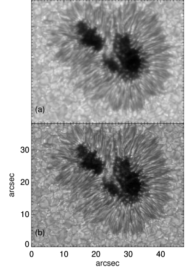
Figure 2.— Sunspot in NOAA AR 12227 shown before (a) and after (b) stray-light correction. Both images in the top and bottom panels have the same intensity scale.

2.2. Sunspot epoch, decay and growth rate

Full-disk HMI continuum images were used to determine the macro-properties of the sunspots. Prior to estimating the sunspot area, the images were corrected for geometric foreshortening in the following manner. The position of each pixel on the solar disk was defined in terms of the position angle $\theta_{i}=\tan^{-1}(x_{i}/y_{i})$ and the radial distance $\rho_{i}=\sqrt{x^{2}_{i}+y^{2}_{i}}$, where $x_{i}$ and $y_{i}$ represent the position of $i^{th}$ pixel on the surface of the Sun measured from disc center. The heliographic coordinates (B and L), were calculated from the following equations:

$$B=\sin^{-1}\{\sin{B_{0}}\cos\rho+\cos{B_{0}}\sin\rho\cos(P-\theta_{i})\}$$ (1)

$$L=\sin^{-1}\Big{\{}\frac{\sin\rho_{i}\cos(P-\theta_{i})}{\cos{B}}\Big{\}}+L_{0}$$ (2)

$$\rho=\sin^{-1}\Big{\{}\frac{\rho_{i}}{S}\Big{\}}-\rho_{i},$$ (3)

where S is the radius of the Sun in arcsec and P is the equatorial horizontal parallax angle. Once the heliographic coordinates for each pixel were known they were transferred to a two-dimensional (2D) image defined by latitude and longitude. This process was carried out on all HMI continuum images for the selected sunspots. The HMI filtergrams were normalized with the QS intensity at disc centre.

Before calculating the sunspot area, the intensity corresponding to the umbra-penumbra boundary and the penumbra-QS boundary was determined using the cumulative intensity histogram method (Pettauer & Brandt, 1997). The intensity threshold for the umbra-penumbra and penumbra–QS boundaries were estimated to be 0.5I_QS and 0.9I_QS, respectively. The variation of the spot area with time was used to determine the decay or growth rate using a linear fit (Chapman et al., 2003). The area change of a sunspot as a function of time can be expressed as, $\mathrm{A(T)=m\times(T-T_{0})+A_{0}}$, where $m$ yields the decay or growth rate and $A_{0}$ is the maximum area of a decaying spot (minimum in the case of a growing spot). From the above expression, the time when the area of a decaying spot reduces to zero works out to be $\mathrm{T_{n}=A_{0}/m}$, where $\mathrm{T_{0}}$ is the time when the area of a decaying sunspot is maximum (minimum in case of growing spot) on the solar disk. In order to relate the macro-properties of a sunspot with the physical characteristics of UDs, we determined the epoch of a decaying spot as the ratio of the Hinode observing time ($\mathrm{T_{H}}$) to the time when the spot area reduces to zero ($\mathrm{T_{n}}$), whereas for the growing spot it is defined as the ratio of the Hinode observing time ($\mathrm{T_{H}}$) to the time when the spot area is maximum. As an example, the decay rate of a sunspot in NOAA AR 11974 is shown in Fig. 3. The area rate of change and epoch of the spots are described in the sixth and seventh columns of Table 2, respectively.

Figure 3.— Temporal evolution of an umbral area.. The filled circles represents the area of the umbra (NOAA AR 11974) and the solid line is a linear fit. A grey dotted line indicates the Hinode observing time (T_H) of the same sunspot.

3. Identification of UDs

The first step in identifying UDs from the Hinode G-band images was to extract the umbral region. The SC images, corresponding to a spatial sampling of 0$\farcs$11 pixel^-1, were smoothed by a 15 pixel $\times$ 15 pixel boxcar (a 7.5 pixel $\times$ 7.5 pixel boxcar was used for spots with a coarser spatial sampling) and the umbra was extracted using the cumulative histogram method employed earlier for the HMI images. This yielded a value of 0.35I_QS corresponding to the umbra-penumbra boundary in the Hinode G-band images. The identification of UDs was carried out using a 2D multi-level tracking (MLT; Bovelet & Wiehr, 2001) algorithm that has been implemented by Riethmüller et al. (2008) and Louis et al. (2012a). This algorithm works in the following manner. The intensity range in the umbra is binned into several levels chosen by the user and the algorithm identifies UDs at each intensity level starting from the highest to the lowest intensity level. All UDs corresponding to the maximum intensity in the umbra are tagged uniquely. Then, the intensity threshold is reduced to the next lower level and the UDs are identified once again, with the previously identified structures retaining their tagged number. This process continues until the last intensity level is reached. The number of UDs detected increases with the number of intensity levels defined in MLT algorithm.

In order to optimize the MLT algorithm for our dataset, the number of intensity levels was varied between 10 to 45 in steps of 5 and the corresponding values of the physical parameters were noted. We observed that although the number of UDs detected, increased by a factor of about 1.5 when the number of intensity levels changed from 25 to 45, the average value of the physical parameters remained unchanged and the overall variation for different sized-sunspots was nearly similar at and above 25 intensity levels. Furthermore, a visual inspection was carried out to verify if the algorithm identified all discernible UDs for a given number of levels. With 10 intensity levels, obvious UDs go undetected, while with 45 levels the algorithm primarily detects smaller and diffuse structures, whose inclusion does not alter the final statistical results. A final test was performed, with a smaller sample of sunspots, spanning 10″ to 40″ in diameter, and it was found that the final results were unaffected. This test was also carried out for different number of intensity levels and the outcome was similar to the one described above. These tests allowed us to finally select 25 intensity levels for the MLT routine.

Once the UDs are identified by the MLT routine, the boundary of each UD is defined by a contour which corresponds to 50% of its maximum and background intensity, i.e., (I_max + I_bg)/2. The background umbral image is determined by smoothing the original image with a 7 pixel $\times$ 7 pixel boxcar window. Figure 4 shows the extraction of an umbra from a sunspot and the location of UDs identified using the MLT algorithm.

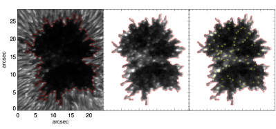
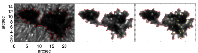
Figure 4.— Top panels: Stray-light corrected image of a sunspot observed in NOAA AR 11921 where the red contour outlines the umbra–penumbra boundary (left), the isolated umbra from the sunspot (middle), and the isolated umbra with the locations of the UDs indicated by yellow plus symbols after employing the MLT algorithm with 25 intensity levels (right). Bottom panels: Same as top panels but for NOAA AR 11974.

Table 2Physical properties of UDs determined from the Hinode stray-light corrected images. Columns 2–6 correspond to the mean intensity (I_mean/I_QS), maximum intensity (I_max/I_QS), the mean effective diameter (D_eff), total number of umbral dots (UD $\#$), and the filling factor (ff), respectively. The seventh and eighth columns represent the area change in the selected sunspots and epoch, respectively which were estimated from HMI/SDO continuum images. The values in the parentheses represent the $rms$ value.

Spot	Imean/IQS	Imax/IQS	Deff	UD	ff	Area change	epoch
No.			(″)	$\#$	(%)	106 $\times$ Km2/day
1	0.23 (0.09)	0.26 (0.11)	0.64 (0.14)	24	6.3	10.63 (2.35)†	0.054
2	0.27 (0.07)	0.30 (0.09)	0.35 (0.07)	52	5.5	113.06 (26.57)†	0.188
3	0.30 (0.18)	0.36 (0.25)	0.51 (0.14)	33	3.4	110.04 (23.06)†	0.262
4	0.21 (0.07)	0.24 (0.09)	0.57 (0.11)	15	6.5	36.44 (3.55)†	0.383
5	0.17 (0.09)	0.20 (0.11)	0.69 (0.16)	33	6.0	68.07 (19.90)⟂	0.507
6	0.22 (0.15)	0.26 (0.19)	0.64 (0.15)	27	5.6	47.78 (4.06)†	0.087
7	0.18 (0.14)	0.21 (0.18)	0.68 (0.17)	37	4.8	53.80 (10.97)†	0.097
8	0.21 (0.13)	0.25 (0.15)	0.55 (0.17)	128	3.5	9.34 (4.66)⟂	0.073
9	0.18 (0.06)	0.21 (0.07)	0.47 (0.15)	77	4.5	57.99 (9.07)†	0.244
10	0.16 (0.06)	0.19 (0.08)	0.49 (0.17)	49	6.2	95.77 (14.42)⟂	0.521
11	0.24 (0.12)	0.28 (0.15)	0.46 (0.08)	49	6.0	29.82 (3.22)†	0.225
12	0.18 (0.09)	0.22 (0.12)	0.83 (0.32)	114	5.3	42.58 (3.19)†	0.101
13	0.20 (0.06)	0.24 (0.08)	0.69 (0.21)	47	6.0	54.65 (10.42)†	0.046
14	0.22 (0.11)	0.25 (0.14)	0.50 (0.12)	82	6.1	11.02 (1.80)†	0.039
15	0.22 (0.13)	0.26 (0.16)	0.66 (0.14)	21	3.7	31.47 (2.64)†	0.132
16	0.22 (0.13)	0.26 (0.16)	0.74 (0.23)	98	4.1	153.73 (49.73)†	0.034
17	0.22 (0.14)	0.26 (0.18)	0.70 (0.19)	59	3.4	223.40 (28.32)⟂	0.681
18	0.25 (0.14)	0.29 (0.18)	0.54 (0.14)	23	4.1	17.14 (1.61)†	0.099
19	0.21 (0.10)	0.24 (0.14)	0.66 (0.15)	24	5.1	61.01 (6.17)†	0.116
20	0.22 (0.10)	0.24 (0.11)	0.62 (0.18)	10	5.1	69.52 (22.10)†	0.151
21	0.22 (0.15)	0.25 (0.19)	0.58 (0.13)	27	4.4	92.84 (4.66)†	0.049
22	0.19 (0.14)	0.22 (0.17)	0.64 (0.22)	41	5.3	31.56 (2.16)†	0.125
23	0.17 (0.11)	0.19 (0.13)	0.66 (0.16)	28	5.7	37.49 (2.90)⟂	0.572
24	0.15 (0.07)	0.17 (0.10)	0.70 (0.11)	27	5.2	33.12 (2.45)†	0.122
25	0.14 (0.07)	0.16 (0.09)	0.70 (0.16)	23	4.8	12.71 (1.87)†	0.048
26	0.19 (0.08)	0.22 (0.09)	0.57 (0.13)	32	7.0	37.13 (2.35)†	0.170
27	0.14 (0.07)	0.16 (0.07)	0.68 (0.22)	10	3.0	25.14 (1.70)†	0.123
28	0.17 (0.11)	0.20 (0.14)	0.69 (0.18)	11	3.2	23.31 (2.3)⟂	0.233
29	0.28 (0.09)	0.32 (0.12)	0.66 (0.24)	8	5.1	55.84 (5.04)†	0.466
30	0.20 (0.08)	0.22 (0.09)	0.67 (0.16)	22	7.2	73.44 (6.00)†	0.225
31	0.17 (0.08)	0.19 (0.09)	0.58 (0.15)	13	4.5	86.37 (5.26)†	0.310
32	0.20 (0.09)	0.22 (0.10)	0.65 (0.13)	25	5.9	29.72 (2.76)†	0.135
33	0.16 (0.06)	0.18 (0.08)	0.72 (0.14)	21	5.5	11.96 (1.34)†	0.056
34	0.16 (0.07)	0.19 (0.09)	0.70 (0.17)	23	5.6	44.36 (7.44)⟂	0.635
35	0.17 (0.10)	0.19 (0.12)	0.75 (0.11)	20	5.8	26.69 (2.24)†	0.132
36	0.19 (0.07)	0.21 (0.08)	0.66 (0.15)	65	5.6	130.75 (23.23)†	0.302
37	0.11 (0.06)	0.12 (0.07)	0.61 (0.15)	44	4.9	252.80 (38.66)†	0.023
38	0.20 (0.10)	0.22 (0.12)	0.65 (0.16)	45	6.2	38.07 (5.59)†	0.061
39	0.29 (0.21)	0.36 (0.28)	0.84 (0.14)	13	4.5	13.30 (7.51)†	0.042
40	0.21 (0.10)	0.23 (0.12)	0.65 (0.16)	21	5.9	44.47 (12.48)†	0.243
41	0.15 (0.09)	0.16 (0.10)	0.67 (0.15)	22	3.5	137.53 (23.02)†	0.299
42	0.25 (0.16)	0.28 (0.19)	0.38 (0.10)	68	5.8	15.40 (1.49)†	0.098

Notes. ($\perp$) Growing spot. (^†) Decaying spot.

For each UD, we determine its peak intensity and mean intensity over all pixels enclosed by the UD boundary. We assume that the shape of each UD is circular, although they can be elliptical (Kilcik et al., 2012). The effective diameter for each identified UD was calculated as D${}_{\mathrm{eff}}=\sqrt{4A/\pi}$, where $A$ represents the total number of pixels in an UD. Those structures which had an area of greater than 2 pixels were considered for the analysis. We also verified if selecting UDs on the basis of their proximity to the umbra-penumbra boundary had any discernible effect on the final results and we found that neither an ingress of the umbra-boundary, moving from 2 to 8 pixels inwards, nor excluding conspicuous bright peripheral features altered the average value of the physical parameters chosen for our study.

For each sunspot, the mean of the following quantities pertaining to the UDs was determined, namely, maximum intensity, mean intensity, and effective diameter. Hereafter, the term intensity will be used to refer to the average of both the mean and maximum intensity of UDs, unless explicitly mentioned.

4. Results

In this section, we present the physical properties of UDs observed in the umbra of 42 different sunspots, which are summarized in Table 2.

4.1. Umbral size, intensity and number of UDs

The umbrae (D_umb) from the 42 selected sunspots in the Hinode data set varied from 8″ to 40″  in diameter (see Table 1). However, the majority of sunspots had a diameter between 10″and 20″and only 4 sunspots with a diameter between 30″and 40″.

Figure 5.— Left panel: From top to bottom - variation of the mean umbral intensity, number of UDs, and filling factor as a function of the umbral diameter for the stray-light corrected images. Right panel: same as left but for the uncorrected data set. The solid line in the top panels represents a power law fit, while in the middle and bottom panels it corresponds to a linear fit. The linear correlation coefficient between the parameters is indicated by ‘cc’ in the inset.

Panel ‘a’ of Figure 5 shows the relation between the mean intensity in the umbra and umbral diameter for the SC data set. A non-linear relation between the two quantities is clearly evident. The mean intensity in the umbra for all spots varies between 0.08–0.19I_QS. However, in smaller umbrae (D${}_{\mathrm{umb}}<20^{\prime\prime}$) the intensity decreases much faster than in larger umbrae. For D${}_{\mathrm{umb}}>20^{\prime\prime}$ the intensity decreases slowly and linearly. In order to understand this behaviour, the observed distribution is fitted with linear and power law functions. However, we noticed that a power law fit describes this distribution better than a linear fit. The power law describing the non-linear trend is indicated by a solid line and the corresponding parameters are included in Table 3. It is also observed that smaller umbrae are brighter than the bigger ones by a factor of 1.7. In order to verify that the observed trend between the mean umbral intensity and the umbral diameter is not an artifact from the PSF deconvolution, we plot the same for the uncorrected data set as well, which is shown in Panel ‘b’ of Fig. 5. The non-linear trend is clearly visible, although the intensities are much higher, ranging from 0.12–0.24I_QS which would be expected from the uncorrected data set. The plots also show that the slopes for the SC and NC data sets only differ by 10%.

Panel ‘c’ of Fig. 5 demonstrates the relation between the number of UDs (NUDs) and the umbral diameter for the SC images, and it is seen that the NUDs increase with the umbral diameter. To a first order, this scatter can be expressed with a linear fit between the two quantities. The same is observed with the NC images (Panel ‘d’), although the NUDs is marginally smaller than those in the SC images, specifically for spots with umbral diameters larger than 30″. We obtained a strong positive correlation of 0.83 and 0.81 between the two quantities for the SC and NC images, respectively. For spots with umbral diameters less than 15″, the NUDs is less than 50, with a scatter amounting to about 20.

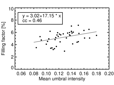
Figure 6.— Scatter plot between filling factor and the mean umbral intensity. The solid gray line is the best linear fit to the observed values. The linear correlation coefficient between the parameters is indicated by ‘cc’ in the inset.

We also determined the fill fraction of UDs as the ratio of the total area occupied by UDs to the umbral area. The fill fraction ranges from 3$\%$–7.2$\%$ (bottom panels of Fig. 5) for all sunspot umbrae. A weak negative correlation coefficient of $-0.3$ and $-0.24$ was observed in the SC and NC images, respectively. Smaller umbrae exhibit a higher fill fraction compared to larger umbrae. In order to see the overall trend, the average fill fraction was determined for umbral diameters within 8″ bins and the solid line in the figure, represents the best linear fit to the average values. The slope of the fit indicates that the fill fraction is nearly independent of the umbral diameter.

A scatter plot in Figure 6 illustrates the relation between the mean umbral intensity and the filling factor. We observe that the filling factor shows a weak positive correlation with the mean umbral intensity. The filling factor increases by a factor of about 1.4 over the range of the mean umbral intensities. We also note that if the number of levels in the MLT routine are increased to 45, the newly detected UDs only reflect an increase in the fill fraction of 1% as compared to the case when 25 levels are used in the detection scheme.

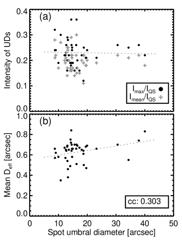
Figure 7.— Top: Scatter plot between UD intensity and umbra diameter. Filled circles and plus symbols represent the maximum and mean UD intensity, respectively. The dashed line represents the best linear fit between the maximum UD intensity and umbra diameter. Bottom: Scatter plot between effective diameter (D_eff) of UDs and umbral diameter. The dashed lines represents the best linear fit between the umbral diameter and D_eff.

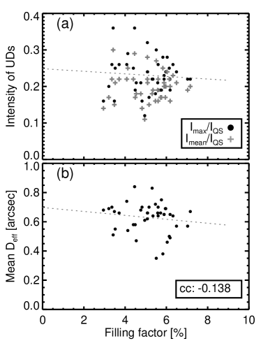
Figure 8.— Same as Fig. 7 but with the filling factor along the abscissa.

4.2. Intensity and size of UDs

The top panel of Fig. 7 shows that the maximum intensity of UDs in the dataset ranges from 0.12 to 0.36I_QS, while the mean intensity of UDs varies from 0.11 to 0.3I_QS.The mean and maximum UD intensity is mainly confined between 0.15–0.3I_QS. The brightest UD in the smallest umbra exceeds that in the biggest umbra by a factor of 1.5. Unlike the power law relation between the size and intensity of the sunspot umbra (Fig. 5a), neither the maximum nor mean intensity of UDs exhibit a correlation with the umbral size as seen in the top panel of Fig. 7. Figure 7(b) shows that the effective diameter of UDs, primarily lies between 0$\farcs$4 to 0$\farcs$7, with minimum and maximum values of 0$\farcs$35 to 0$\farcs$84, respectively. A linear fit to the scatter suggests that UDs dwelling in smaller umbrae are smaller than those found in larger umbrae, with a modest correlation coefficient of about 0.3.

We also do not observe any dependence of the intensity and effective diameter of UDs with the fill fraction (Fig. 8). The bottom panel of Fig. 8 indicates that the effective diameter of UDs, is negatively correlated with the fill fraction, due to the large scatter in the data. The linear fit (Table 3) indicates that for a fill fraction of 10% the effective diameter of UDs would be around 0$\farcs$57.

The mean umbral intensity exhibits a modest correlation with intensity of UDs (Figure 9). We see that the maximum intensity of UDs exceeds the mean umbral intensity by about 10% with a slope of around 0.7.

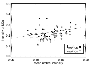
Figure 9.— Scatter plot showing the variation of the maximum and mean intensity of UDs with the mean umbral intensity observed in 42 different umbrae. The dashed line indicates the best linear fit between the maximum UD intensity and mean umbral intensity.

4.3. UD parameters versus the area change and epoch of sunspots

Figure 10 (bottom panels) shows the relation of the effective diameter of UDs (D_eff) with the decay/growth rate and epoch of sunspots. It is observed that the effective diameter of UDs (D_eff) is insignificantly related to both the decay/groth rate and epoch for the 42 sunspots studied here. The bottom left panel of Fig. 10, indicates that a majority of the UDs are associated with sunspots having a slow rate of area change ($<$ 50 Mkm²). Similarly, the bottom right panel of Fig. 10 illustrates that the effective diameter of UDs is also independent of the epoch of sunspots.

Similar to the effective diameter of UDs, the top panels of Fig. 10 demonstrate that the maximum intensity of UDs does not exhibit any trend with the rate of area change and the epoch of sunspots. Even though UDs tend to be brighter when sunspots decay slowly, this variation is less than 5%. The same is valid for the sunspot epoch where the UDs are only a fraction brighter during the early phase of sunspots.

Table 3Fit parameters for the power law (y = A $\times$ x^B; Figures 5(a – b)) and linear (y = A + Bx; Figures 5(c, d, e, f), 6, 7, 8, 9) functions. Abbreviation ‘ff’, ‘I_umb’, and ‘I_UD’ correspond to the filling factor, quiet-sun normalized mean umbral intensity and maximum UD intensity, respectively. In the sixth column ‘cc’ refers to the linear Pearson correlation coefficient between parameters. The numbers in the parenthesis denote one-sigma errors.

Figure	x	y	A	B	CC
5(a)†	Dumb	Iumb	0.38 (0.48)	$-0.40$ (0.45)	$-0.69$
5(b)‡	Dumb	Iumb	0.46 (0.58)	$-0.36$ (0.45)	$-0.78$
5(c)†	Dumb	NUD	$-9.2$ (15.70)	3.44 (0.65)	0.83
5(d)‡	Dumb	NUD	$-11.52$ (14.41)	3.02 (0.60)	0.81
5(e)†	Dumb	ff	5.77 (1.03)	$-0.06$ (0.046)	$-0.30$
5(f)‡	Dumb	ff	5.30 (0.80)	$-0.05$ (0.04)	$-0.24$
6†	Iumb	ff	3.02 (0.71)	17.15 (5.06 )	0.46
7(a)†	Dumb	IUD	0.23 (0.02)	$-2.01(1.14)\times 10^{-4}$	$-0.028$
7(b)†	Dumb	Deff	0.55 (0.04)	$4.44(2.21)\times 10^{-3}$	$0.30$
8(a)†	ff	IUD	0.25 (0.04)	$-3.5(7.6)\times 10^{-3}$	$-0.073$
8(b)†	ff	Deff	0.70 (0.08)	$-0.013$ (0.015)	$-0.138$
9†	Iumb	IUD	0.14 (0.04)	0.70 (0.33)	0.31
10(a)†	$\mathrm{dA/dt}$	I${}_{\mathrm{UD}}^{\mathrm{max}}$	0.24 (0.02)	$-$1.2 (1.4) $\times 10^{-4}$	$-0.131$
10(b)†	Epoch	I${}_{\mathrm{UD}}^{\mathrm{max}}$	0.23 (0.01)	$-$1.8 (4.6) $\times 10^{-4}$	$-0.063$
10(c)†	$\mathrm{dA/dt}$	Deff	0.63 (0.02)	$-$6.13 (3.0) $\times 10^{-5}$	$-0.032$
10(d)†	Epoch	Deff	0.63 (0.02)	$-$1.9 (9.3) $\times 10^{-4}$	$-0.032$

The parameters retrieved from SC and NC images are indicated by ‘${\dagger}$’ and ‘${\ddagger}$’ superscript, respectively. The rate of area change is denoted by $\mathrm{dA/dt}$.

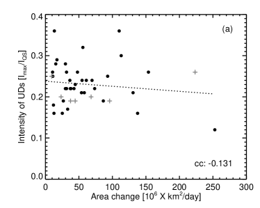
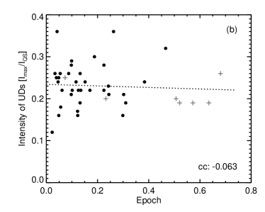
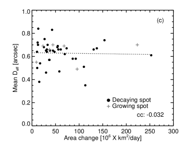
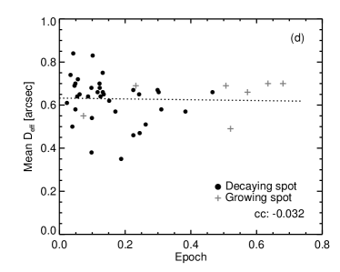
Figure 10.— Top panels: scatter plots depict the relation of maximum intensity of UDs with respect to the sunspot area change, i.e. decay/growth rate (left) and sunspot epoch (right). Bottom panels: same as the top panels but with the effective diameter of UDs along the ordinate. The linear correlation coefficient between parameters is indicated by ‘cc’ and the dashed line denotes the best linear fit.

5. Discussion

Umbral dots are manifestations of small-scale magnetoconvection in sunspots. Our study shows that there is a dependence of the mean umbral brightness with the spot size which is in agreement with Mathew et al. (2007), where smaller spots are brighter than larger ones. This would imply that darker spots comprise stronger magnetic fields which suppress magnetoconvection as suggested by Maltby (1977); Kopp & Rabin (1992); Livingston (2002). Thus, if umbral dots are manifestations of small-scale, magnetoconvection, then one would expect that their physical properties have a bearing on the macro-properties of a sunspot. In the context of Parker’s “jelly-fish” model (Parker, 1979), the energy transport in umbrae ought to be more vigorous during the late phase of sunspots as they approach fragmentation, and the reduced magnetic pressure would be insufficient to overcome the resulting gas pressure. This should be seen as brighter and/or larger umbral dots, that could then be used as a proxy for several large-scale properties of sunspots, namely, their area, rate of decay, and evolutionary phase. With this motivation in mind, we have selected a large set of sunspots and tracked them during their transition across the solar disc. By employing high resolution G-band filtergrams from Hinode, close to disc center, the physical properties of umbral dots were estimated and related to the above mentioned sunspot properties. We have taken care of instrumental stray-light in the Hinode filtergrams, which is known to affect the geometrical and photometric properties of umbral dots (Louis et al., 2012a) and our analysis primarily focuses on the intensity and effective diameter.

We find that a strong linear relationship exists between the number of umbral dots and umbral diameter, which would suggest that in bigger spots there are larger spaces for convection to occur within the umbra. However, the fill fraction of umbral dots is nearly independent of the umbral diameter and accounts for less than 10% of the umbral area, which is in agreement with Sobotka et al. (1993); Sobotka & Hanslmeier (2005). This stems from the fact that the diameter of umbral dots does not show any variation with the spot size. In addition, both the mean and maximum intensity as well as diameter of umbral dots do not show any visible trend with the area decay rate and the spot epoch either, exhibiting very weak, negative correlations. We find, that although UDs tend to be brighter during the late phase of sunspots, this variation is less than 5%. We also observed a similar behavior with the rate of area change. We also see that UDs tend to be smaller for spots that are either in an advanced stage of evolution or decay faster. This is reflected in a negative, although very weak, correlation coefficient. Our results show that the maximum intensity of UDs is about 10% brighter than the mean umbral intensity. We interpret this as a combined effect of the small fill fraction of less than 10% and the weak dependence between the diameter of UDs and the host umbra. This would indicate that the dependence of umbral intensity with the spot size originates primarily from the background regions of the umbra and to a very small fraction from UDs. The lack of a relationship between the properties of umbral dots and the macro-properties of the parent spots is discussed below.

In addition to umbral dots, light bridges represent large-scale, convective intrusions in the umbrae of sunspots and pores (Muller, 1979; Sobotka et al., 1994; Lites et al., 2004; Louis et al., 2008, 2009). The association between these two phenomena has been established in several works (Garcia de La Rosa, 1987; Hirzberger et al., 2002; Rimmele, 2008). Katsukawa et al. (2007) studied the formation of sunspot light bridge using Hinode observations. They found that the formation was preceded by an inward motion of umbral dots that appeared well within the umbra and not the penumbra. They interpreted this observation as a sign of the weakening of the magnetic field by the hot rising plasma that then allowed several umbral dots from the leading edges of penumbral filaments to intrude further into the umbra, forming a light bridge out of a collection of umbral dots. The formation of a light bridge is associated with a rapid increase of intensity, from umbral to penumbral values in about 4 hr, which is accompanied by a large reduction in the field strength (Louis et al., 2012b). In light of the above, the lack of trend between the umbral dot size and the spot area suggests that the interaction of the magnetic field and convection, within the umbra, occurs over a set of distinct, interchangeable spatial scales. Thus, depending on the underlying conditions of the magnetic and gas pressure, umbral dots would coalesce to form light bridges during late stages of spot decay and light bridges would disintegrate into umbral dots during the spot’s maturity (see for example Fig.2 of Schlichenmaier et al., 2010). Since the contribution of light bridges to the intensity of umbral dots was excluded in our analysis, it would be necessary to determine how these structures influence the size and intensity of the latter.

Another possibility of the lack of any discernible relation between the intensity and diameter of umbral dots with the spot size, could be attributed to the shallow depth to which these structures extend to. MHD simulations of magnetocovnection in the umbra by Schüssler & Vögler (2006), show that umbral dots correspond to vertically rising convective plumes from a depth of around 2 Mm, while light bridges extend a little deeper to around 6–7 Mm (Cheung et al., 2010). Even with this simulation depth, the photospheric properties of light bridges are in good agreement with those typically seen in observations. These depths only represent a small fraction of the solar convection zone which is strongly stratified by 6 orders of magnitude over a depth of 200 Mm (Christensen-Dalsgaard et al., 1991). This poses an enormous computational challenge, and as such numerical models focus either on the deep convection zone leaving out the uppermost 10–20 Mm or on the uppermost 10 Mm including the solar photosphere.

According to Schüssler & Rempel (2005), during the final phase of the ascent of a rising flux loop towards the surface, the upper part of the loop develops a buoyant upflow of plasma. The combination of the pressure build-up by the upflow and the cooling of the upper layers of an emerged flux tube by radiative losses at the surface leads to a progressive weakening of the magnetic field at depths of several Mm, which can lead to a dynamic disconnection of the bipolar structure from its magnetic roots. The disconnection depth extends to a few tens of Mm as shown by Švanda et al. (2009), but is associated with only one-third of the sample analyzed. Similar values of the disconnection depth have been reported by Maurya & Ambastha (2010) who find a linear relation of the above with the remaining lifetime of active regions. This would suggest that umbral dots and light bridges are strongly influenced by near-surface convective flows, rather than those which are associated with the severing of sunspots from their roots, which occur much deeper.

6. Conclusions

The study of umbral dots with high-resolution data is crucial for understanding small-scale magnetoconvection in sunspot umbrae, that can constrain existing sunspot models in a more robust manner. In this article, we have attempted to relate the physical properties of umbral dots with the large-scale properties of sunspots, in order to determine if the underlying physical processes, that influence the evolution and stability of the latter, are indeed scale-invariant. We do not find any significant relationship between the effective diameter of umbral dots with the sunspot area, epoch, and decay rate. The same is observed with the mean and maximum intensity of the umbral dots. We conclude that the above could either be due to the distinct transition of spatial scales associated with overturning convection in the umbra, where umbral dots can coalesce to form light bridges, or the shallow depth associated with umbral dots which make them impervious to the deeper, large-scale, convective flows that affect the anchoring of sunspots, or both of the above. We intend to investigate if this lack of trend is extended to sunspots over an entire solar cycle and with spots that have an umbral radius greater than 25″. Facilities such as the 1.5-m GREGOR solar telescope (Schmidt et al., 2012) and the 4-m Daniel K. Inoyue Solar Telescope (DKIST, formerly ATST; Keil et al., 2003) will be extremely important in these investigations as spatially resolved UDs would allow improved statistics by providing evidence of magnetoconvection at the smallest spatial scales.
Acknowledgements: Hinode is a Japanese mission developed and launched by ISAS/JAXA, collaborating with NAOJ as a domestic partner, NASA and STFC (UK) as international partners. Scientific operation of the Hinode mission is conducted by the Hinode science team organized at ISAS/JAXA. This team mainly consists of scientists from institutes in the partner countries. Support for the post-launch operation is provided by JAXA and NAOJ (Japan), STFC (U.K.), NASA, ESA, and NSC (Norway). The HMI data used here are courtesy of NASA/SDO and the HMI science team. The Center of Excellence in Space Sciences India is funded by the Ministry of Human Resource Development, Government of India. REL is grateful for the financial assistance from SOLARNET–the European Commission’s FP7 Capacities Programme under Grant Agreement number 312495. This work was also supported by grants AYA2014-60476-P and SP2014-56169-C6-2-R at the Instituto de Astrofísica de Canarias, Tenerife, Spain. We thank the referee for reviewing our article and for providing insightful comments.

References

- Bovelet & Wiehr (2001) Bovelet, B., & Wiehr, E. 2001, Sol. Phys., 201, 13
- Chapman et al. (2003) Chapman, G. A., Dobias, J. J., Preminger, D. G., & Walton, S. R. 2003, Geophysical Research Letters, 30, n/a, 1178. http://dx.doi.org/10.1029/2002GL016225
- Cheung et al. (2010) Cheung, M. C. M., Rempel, M., Title, A. M., & Schüssler, M. 2010, ApJ, 720, 233
- Christensen-Dalsgaard et al. (1991) Christensen-Dalsgaard, J., Gough, D. O., & Thompson, M. J. 1991, ApJ, 378, 413
- Garcia de La Rosa (1987) Garcia de La Rosa, J. I. 1987, Sol. Phys., 112, 49
- Grossmann-Doerth et al. (1986) Grossmann-Doerth, U., Schmidt, W., & Schroeter, E. H. 1986, A&A, 156, 347
- Hamedivafa (2011) Hamedivafa, H. 2011, Sol. Phys., 270, 75
- Hirzberger et al. (2002) Hirzberger, J., Bonet, J. A., Sobotka, M., Vázquez, M., & Hanslmeier, A. 2002, A&A, 383, 275
- Katsukawa et al. (2007) Katsukawa, Y., Yokoyama, T., Berger, T. E., et al. 2007, PASJ, 59, S577
- Keil et al. (2003) Keil, S. L., Rimmele, T., Keller, C. U., et al. 2003, in Proc. SPIE, Vol. 4853, Innovative Telescopes and Instrumentation for Solar Astrophysics, ed. S. L. Keil & S. V. Avakyan, 240–251
- Kilcik et al. (2012) Kilcik, A., Yurchyshyn, V. B., Rempel, M., et al. 2012, ApJ, 745, 163
- Kitai et al. (2007) Kitai, R., Watanabe, H., Nakamura, T., et al. 2007, PASJ, 59, 585
- Kopp & Rabin (1992) Kopp, G., & Rabin, D. 1992, Sol. Phys., 141, 253
- Kosugi et al. (2007) Kosugi, T., Matsuzaki, K., Sakao, T., et al. 2007, Sol. Phys., 243, 3
- Lites et al. (2004) Lites, B. W., Scharmer, G. B., Berger, T. E., & Title, A. M. 2004, Sol. Phys., 221, 65
- Livingston (2002) Livingston, W. 2002, Sol. Phys., 207, 41
- Louis et al. (2008) Louis, R. E., Bayanna, A. R., Mathew, S. K., & Venkatakrishnan, P. 2008, Sol. Phys., 252, 43
- Louis et al. (2009) Louis, R. E., Bellot Rubio, L. R., Mathew, S. K., & Venkatakrishnan, P. 2009, ApJ, 704, L29
- Louis et al. (2012a) Louis, R. E., Mathew, S. K., Bellot Rubio, L. R., et al. 2012a, ApJ, 752, 109
- Louis et al. (2012b) Louis, R. E., Ravindra, B., Mathew, S. K., et al. 2012b, ApJ, 755, 16
- Lucy (1974) Lucy, L. B. 1974, AJ, 79, 745
- Maltby (1977) Maltby, P. 1977, Sol. Phys., 55, 335
- Mathew et al. (2007) Mathew, S. K., Martínez Pillet, V., Solanki, S. K., & Krivova, N. A. 2007, A&A, 465, 291
- Mathew et al. (2009) Mathew, S. K., Zakharov, V., & Solanki, S. K. 2009, A&A, 501, L19
- Maurya & Ambastha (2010) Maurya, R. A., & Ambastha, A. 2010, ApJ, 714, L196
- Muller (1979) Muller, R. 1979, Sol. Phys., 61, 297
- Parker (1979) Parker, E. N. 1979, ApJ, 234, 333
- Pesnell et al. (2012) Pesnell, W. D., Thompson, B. J., & Chamberlin, P. C. 2012, Sol. Phys., 275, 3
- Pettauer & Brandt (1997) Pettauer, T., & Brandt, P. N. 1997, Sol. Phys., 175, 197
- Richardson (1972) Richardson, W. H. 1972, Journal of the Optical Society of America (1917-1983), 62, 55
- Riethmüller et al. (2008) Riethmüller, T. L., Solanki, S. K., Zakharov, V., & Gandorfer, A. 2008, A&A, 492, 233
- Rimmele (2008) Rimmele, T. 2008, ApJ, 672, 684
- Scherrer et al. (2012) Scherrer, P. H., Schou, J., Bush, R. I., et al. 2012, Sol. Phys., 275, 207
- Schlichenmaier et al. (2010) Schlichenmaier, R., Rezaei, R., Bello González, N., & Waldmann, T. A. 2010, A&A, 512, L1
- Schmidt et al. (2012) Schmidt, W., von der Lühe, O., Volkmer, R., et al. 2012, Astronomische Nachrichten, 333, 796
- Schüssler & Rempel (2005) Schüssler, M., & Rempel, M. 2005, A&A, 441, 337
- Schüssler & Vögler (2006) Schüssler, M., & Vögler, A. 2006, ApJ, 641, L73
- Sobotka et al. (1993) Sobotka, M., Bonet, J. A., & Vazquez, M. 1993, ApJ, 415, 832
- Sobotka et al. (1994) —. 1994, ApJ, 426, 404
- Sobotka et al. (1997) Sobotka, M., Brandt, P. N., & Simon, G. W. 1997, A&A, 328, 682
- Sobotka & Hanslmeier (2005) Sobotka, M., & Hanslmeier, A. 2005, A&A, 442, 323
- Solanki (2003) Solanki, S. K. 2003, A&A Rev., 11, 153
- Tsuneta et al. (2008) Tsuneta, S., Ichimoto, K., Katsukawa, Y., et al. 2008, Sol. Phys., 249, 167
- Švanda et al. (2009) Švanda, M., Klvaňa, M., & Sobotka, M. 2009, A&A, 506, 875
- Watanabe (2014) Watanabe, H. 2014, PASJ, 66, S1
- Watanabe et al. (2012) Watanabe, H., Bellot Rubio, L. R., de la Cruz Rodríguez, J., & Rouppe van der Voort, L. 2012, ApJ, 757, 49
- Watanabe et al. (2009) Watanabe, H., Kitai, R., & Ichimoto, K. 2009, ApJ, 702, 1048
- Weiss (2002) Weiss, N. O. 2002, Astronomische Nachrichten, 323, 371