Are Cold Dynamical Dark Energy Models Distinguishable in the Light of the Data?

Abstract

In this paper we obtain observational constraints on three dynamical cold dark energy models ,include PL , CPL and FSL, with most recent cosmological data and investigate their implication for structure formation, dark energy clustering and abundance of CMB local peaks. From the joint analysis of the CMB temperature power spectrum from observation of the Planck, SNIa light-curve, baryon acoustic oscillation, $f\sigma_{8}$ for large scale structure observations and the Hubble parameter, we find that $\Omega_{\rm DE}=0.6862\pm 0.0078$, $\alpha=0.1013\pm 0.0031$ and $w_{0}=-1.3799^{+0.0036}_{-0.0028}$ for the PL model, $\Omega_{\rm DE}=0.6880^{+0.0100}_{-0.0079}$, $w_{0}=-1.08045^{+0.00041}_{-0.00062}$ and $w_{1}=-0.12190^{+0.00050}_{-0.00030}$ for the CPL model and $\Omega_{\rm DE}=0.6893\pm 0.0078$, $w_{0}=-0.9994\pm 0.0076$ and $w_{1}=-0.0082^{+0.0044}_{-0.0051}$ for the FSL model at $1\sigma$ confidence interval. The PL model has matter-like contribution to the energy content of early universe due to crossing behavior of its Equation of state. Therefore, the PL model has the highest growth of matter density, $\Delta_{m}$, and matter power spectrum, $P(k)$, compared to $\Lambda$CDM and other models. For the CPL on the other hand, the structure formation is considerably suppressed while the FSL has behavior similar to standard model of cosmology. Studying the clustering of dark energy, $\Delta_{DE}$, yields positive but small value with maximum of $\Delta_{DE}\simeq 10^{-3}$ at early time due to matter behaviour of the PL, while for the CPL and FSL cross $\Delta_{DE}=0$ several time which demonstrate void of dark energy with $\Delta_{DE}\simeq-10^{-11}$ in certain periods of the history of dark energy evolution. Among these three models, the PL model demonstrate that is more compatible with $f\sigma_{8}$ data. We also investigated a certain geometrical measure, namely the abundance of local maxima as a function of threshold for three DDE models and find that the method is potentially capable to discriminate between the models, especially far from mean threshold. The contribution of PL and CPL for late ISW are significant compared to cosmological constant and FSL model. The tension in the Hubble parameters is almost alleviated in the PL model.

1.  Introduction

The accelerating expansion of the universe was first noticed by Riess et al. [1] in High-redshift Supernova Search Team and by Perlumuter et al. [2] in Supernova Cosmology Project Team, independently. After that, many scientific projects have been established in order to asses the source of this phenomenon as well as to achieve desired observational accuracy. Several observational achievements including Cosmic Microwave Background Anisotropy (CMB), Large Scale Structure (LSS), Baryonic Acoustic Oscillations (BAO) and indirect estimations for the Hubble parameter versus redshift also strongly support mentioned dynamics of our cosmos on large scales with high precision [3, 4]. In spite of considerable researchers focused on the nature of this accelerated expansion, there are many challenges in clarifying the corresponding source(s). The historically well known possibility is cosmological constant (CC), so-called concordance model. Although being a greatly successful scenario with high value of confidence interval, $\Lambda$CDM model suffer some problems are still pending to resolve. Among them are the sharp transition from the cold dark matter era to $\Lambda$ dominant epoch and fine tuning problems [5, 6]. In addition, has also been recent report on flowing tension: the excessive congestion of matter and the missing satellites puzzle [7, 8], the cusp-core problem [9, 10, 11] and in a reliable observational projects run by the $Planck$ collaboration, the observed clusters are fewer than expected [12].

From a robust point of view, there are three approaches beyond the$\Lambda$CDM model to elucidate accelerating epoch: The first approach are theoretical orientation and phenomenological dark fluids resulting in dynamical dark energy (DDE) also known as quintessence [13], non canonical scalar field (k-essence) [14], phantom [15], coupled dark energy [16] and so on. The second approach devoted to modification of gravity such as $f(R)$ gravity [17, 18], scalar-tensor theories [19, 20]. The third approach, dedicated to thermodynamics point of view to propose phenomenological exotic fluids [21, 23, 25, 26, 27, 28, 22, 24]. Although, a more recent theory of Uber Gravity devoted to ensemble average on all consistent models of gravity [29, 30]. In this work we focus on DDE models.

Reconstruction of equation of state is another viewpoint based on observations including parametric and non-parametric approaches. Parametric reconstruction is based upon estimation of model parameters from different observational data sets [31], while in non-parametric reconstruction , find nature of cosmic evolution from observation rather than any prior assumptions of parametric from any cosmological parameters. [32, 33, 34].

Since CC equation of state is precisely $w=-1$ and recent data slightly favorite $w<-1$, small deviation from CC allow one to consider models with $w\neq-1$. According to constant nature of CC, it is contributed directly on background evolution. Any conceivable assessment of DDE model needs to incorporate not only the characterizing background evolution but also various aspect of perturbations leading to structure formation affected by DDE. The robust perturbations analysis may provide opportunity to discriminate various scenarios for dark energy. It is worth noting that, the nature of dark energy can be investigated not only by corresponding equation of state but also through sound speed and associated clustering. The measurement of $3D$ gravitational perturbation of galaxy redshift survey at enough large scale suggested for probing of dark energy clustering. Dark energy both clustering individually and cluster together with matter at large spacial scale [35]. At late time, it is found that clustering (overdensity) of matter correspond to void (underdensity) of dark energy, conversely a void in matter was seen produce a local DDE overdensity [36]. Furthermore, for $w<-1$ dark energy void expected and $w>-1$ dark energy cluster happened [37] howbeit there are analysis which $\Delta_{DE}>0$ occur for $w>-1$ [36, 38]. The signature of cold dark energy on galaxy cluster abundance explored [39].

A key question in dealing with model of dark energy family, is finding the realistic scenario. Practically, the proposed models to explain the accelerating expansion of the universe are not distinguishable from $\Lambda$CDM at the level of background expansion history, but hopefully, considering structure formation even at linear regime would lead to different consequences. Currently, precision limitation on current observational data prevent to achieve discrimination between the models. Meanwhile, there are many attempts dedicated to mentioned goal that use most recent high resolution observations in one hand, and introducing curious criteria ranging from new observables to robust topological and geometrical measures in another hand [40, 41, 42]. In methods such as State-finder [43] and Om diagnostic [44], the corresponding parameters are not observable quantities. Part of current data such as ISW and the matter power spectrum do not have enough precision to rule out models with behaviors similar to $\Lambda$CDM. The forthcoming observations designed to constrain the growth function are very promising[45]. Future galaxy weak lensing experiments such as the Dark Energy Survey (DES) [46] and Euclid [47] and SKA project [48] will potentially be able to discriminate between the $\Lambda$CDM and evolving dark energy scenarios. Future CMB in the microwave to far-infrared bands in the polarization and the amplitude, as the Polarized Radiation and Imaging Spectroscopy (PRISM) [49] and the very high precision measurements of the polarization of the microwave sky by the Cosmic Origins Explorer (CoRE) satellite [50] will improve the constraints of the dark sector [51].

The focus of this paper is on parametric reconstruction of some equation of states for DDE. The models chosen in this work have equation of states which behave quite diversity. The Chavelier-Polarski-Linder (CPL) and Feng-Shen-Li (FSL) models remain always below and above $w=-1$ respectively. On the other hand Power Law (PL) model has a crossing $w=-1$ behavior. The CPL model despite being widely used for long time, suffer from divergence as $z$ approach to -1. The alternative divergence-less model is FSL as $z$ approach to -1 instead of CPL proposed. The PL, on the other hand was proposed to resolve fine-tuning problem. Thanks to its crossing behavior, the model has a positive equation of state at early time. Leading it to naturally behave similar to coupled dark energy-Dark matter models without introducing any coupling parameter.

In this work, from observational points of view, we will rely on the state-of-the-art observational data sets such as supernova type Ia (SNIa), baryonic acoustic oscillation (BAO), Hubble parameter, full sky CMB and also take into account the perturbations to examine the consistency of our models with Large Scale Structure (LSS) observables. We introduce a new geometrical measure, namely number density of local maxima as discriminator between different DDE models. We also study perturbation of dark energy and its clustering again a potentially powerful tool to distinguish between various DDE models. Apart from the background field that drives the accelerating expansion of the universe, dark energy perturbations exist intrinsically. The dark energy clustering is relevant not only for structure formation at low redshifts $z\leq 1$, where the energy density dominates of the cosmic expansion, but also for early structure formation when early dark energy exists. A reasonable DDE model with its perturbation predicts that the dark energy can either cluster or produce voids. However, dark energy is smooth on small scales leading small scales structure such as galaxy formation and solar-system dynamics unaffected [35]. We also investigate the implication of these DDE models for structure formation $f\sigma_{8}$ measurement, matter power spectrum and ISW effect and how they improve the Hubble tension.

The paper is organized as follows. In Sec. 2 we describe our phenomenological uncoupled DDE models . In Sec. 3 the theoretical framework of structure formation in present of DDE models will be discussed. These including evolution of scalar perturbation, Power spectrum of matter density, $\sigma_{8}$ and bias free parameter namely $f\sigma_{8}$ as a function of redshift will be included in this section. ISW are also given in Sec. 3. Sec. 4 is devoted to the clustering of DDE models. Sec. 5 introduce a new geometrical measure of the number density of local maxima at the CMB maps in the presence of DDE models which may alter the CMB fluctuations even in very weak situation. Observational constraints based on JLA data sets, BAO, Planck TT, LSS will be given in Sec. 6. Results and discussion about our finding will be given in Sec. 7. We will give concluding remarks in Sec. 8.

2.  Dynamical Dark Energy Models

The nature of agent acceleration is still pending. To this end, various dark energy models as alternative models for cosmological constant have been introduced. A well-known category including a modification on constituent of universe is so-called phenomenological model. This class is devoted to models with rolling fields [52], modified kinetic terms [53] and higher spin fields[54]. In phenomenological approaches, dark energy is mainly characterized by its equation of state $w=p/\rho$, speed of sound $c_{s}^{2}=\delta p/\delta\rho$ and anisotropy stress $\sigma$ [55]. It turns out that DDE models can be distinguished from cosmological constant by time dependence equation of state and non-zero sound speed . The number of free parameters of DDE models depend on theoretical and phenomenological approaches are utilized for construction. However, it was revealed that to achieve decorrelate compression and to avoid crippling limitation, we need at least three free parameters [56].

In this section, we will briefly explain three dark energy models considered for examining clustering of dark energy in the context of perturbation theory. Such dark energy models can be modeled by a barotropic perfect fluid, namely, its pressure just can be considered as a function of density with a proper equation of state depending on redshift. As following, the DDE models have various behavior versus redshift in comparison with $\Lambda$CDM. PL has Phantom-crossing manner which leads similar behavior to dark matter at early time. The FSL model remains always higher than $-1$, while CPL remains less than $-1$. Subsequently, one can asses such classification in the clustering behavior (see Fig. 1).

2.1.  CPL model

The first order covariant expansion for equation of state is $w(z)=w_{0}+w_{1}z$ which is unstable at high redshift. Hence to resolve this problem, Chavelier-Polarski-Linder model (CPL) has been proposed equation of state in the form of [57, 58]:

$$w_{\rm CPL}(z)=w_{0}+w_{1}\dfrac{z}{1+z}$$ (2.1)

where $w_{0}$ and $w_{1}$ are the parameters of equation of state at present time and derivative of equation of state with respect to scale factor, respectively. Several advantage of this model are explored such as manageable two dimensional phase space, bounded behavior at high redshift and reconstruction of many scalar field equation of states with high accuracy. In addition, it possesses fine physical interpretation. Beside mentioned advantages, its equation of state diverge at $z=-1$ [59]. Recent observational consistency test based on supernova revealed that there is no significant evidence of any deviation from linearity from with respect to scale factor [60].

2.2.  FSL model

As mentioned before, CPL model suffers divergence problem when redshift approaches to $z\to-1$ leading to non-physical future. Hence Feng-Shen-Li (FSL) proposed a model to eliminate this problem with non-infinite limit as [61]

$$w_{\rm FSL}(z)=w_{0}+w_{1}\frac{z}{1+z^{2}}$$ (2.2)

The free parameters are similar to CPL model.

2.3.  PL model

Another model utilized for evaluation of dark energy is power-law (PL) parameterized model proposed in order to solve fine tuning problem as [62]:

$$w_{\rm PL}(z)=\frac{w_{0}}{(1+z)^{\alpha}}[1-\alpha\ln\left(1+z\right)]$$ (2.3)

in which $w_{0}$ and $\alpha$ are model’s free parameters. The ratio of the dark energy density to the matter density is not sensitive to value of model’s free parameters and asymptotically goes to zero at early epoch. Hence dark energy does not need to be fine tuned at $t\rightarrow 0$. PL model also solved age of old stars problem which is called cosmic age crisis [62] (for full review of the cosmic age see [63]). Another advantage of the model is that for scale factor in range of $a\propto e^{\frac{1}{\alpha}}$ the sign of equation of state changes to positive value, so it can be a candidate for unified dark energy-dark matter models scenario.

In Fig. 1, we plot the equation of states associated with the mentioned models. We used best fit values for corresponding free parameters based on different observational data sets to illustrate the behavior of equation of states (see section 6). The PL equation of state crosses the cosmological constant at late time and it almost behaves as matter component at early epoch. In the next section we will rely on the hydrodynamical linear perturbation theory to assess inhomogeneities associated with energy constituents.

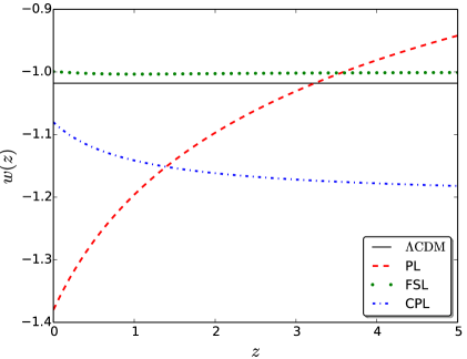
Figure 1: The equation of states of the DDE models as function of redshift. The value of free parameters set to their best fit values determined by observational constraints using by SNIa+BAO+HST+$Planck$ TT+LSS (see section 6).

3.  Structure Formation in DDE I: Standard approach

In this section, we will explain useful theoretical framework to elaborate perturbative dynamics for components universe. First order perturbation on various components and associated velocity dispersion will be discussed in this section. We ignore any interaction between dark sectors of the universe.

3.1.  Evolution of Scalar Perturbation

In order to realize the evolution of perturbation in cold dark matter (CDM) and in a typical DDE component in the framework of perturbation approach, one can decompose the Einstein tensor, $G_{\mu\nu}$, and the energy-momentum tensor, $T_{\mu\nu}$, into background and perturbed parts. A general functional form for $T_{\mu\nu}$ considered as:

$$T_{\mu\nu}=T_{\mu\nu}^{\rm{m}}+T_{\mu\nu}^{\rm{rad}}+T^{\rm{DE}}_{\mu\nu},$$ (3.1)

here $T^{\rm{m}}_{\mu\nu}$, $T^{\rm{rad}}_{\mu\nu}$ and $T^{\rm{DE}}_{\mu\nu}$ are the energy-momentum tensors of the matter, radiation and dark energy, respectively. Tensor $T^{\rm{DE}}_{\mu\nu}$ includes other sources of gravity such as scalar fields [15]. In this paper for the dark energy part, we assume that $w_{\rm DE}$ takes one of DDE model’s equation of state which introduced in previous section. The generalized equation of state reads as:

$$\bar{w}_{i}(a)\equiv\frac{\int_{1}^{a}w_{i}(a^{\prime})d\ln a^{\prime}}{\int_{1}^{a}d\ln a^{\prime}},$$ (3.2)

here $w_{i}$ is equation of state of $i$th component. As an illustration for a given DDE models, $w_{\rm DE}$ is represented by Eqs. (2.1), (2.3) and (2.2). The functional form of generalized equation of state for CPL, FSL and PL are:

$$\bar{w}_{\rm CPL}(a) = \omega_{1}+(\omega_{0}-\omega_{1})\frac{a-1}{\ln(a)},$$ (3.3)

$$\bar{w}_{\rm FSL}(a) = \omega_{0}-\omega_{1}\frac{\arctan\left(\frac{1-a}{a}\right)}{\ln(a)},$$ (3.4)

$$\bar{w}_{\rm PL}(a) = \omega_{0}a^{\alpha}.$$ (3.5)

Considering convention by line element in so-called Newtonian or longitudinal gauge, we get:

$$ds^{2}=a^{2}(\eta)\left[-(1+2\psi)d\eta^{2}+(1-2\phi)dx^{i}dx^{j}\right],$$ (3.6)

where $\eta$ is conformal time, $d\eta=dt/a$. Also $\phi$ and $\psi$ are space-like and time-like variables, respectively describing scalar metric perturbations and known as gauge invariant Bardeen potentials [64]. Gauge fixing influences the perturbations especially on scales larger than Hubble horizon $k\leq aH$, while on much smaller scales the choice of gauge is less important and observables are independent of gauge choice [65].

Hence Einstein perturbed equations and perturbed continuity fluid equation read as:

$$k^{2}\phi+3\mathcal{H}(\phi^{\prime\prime}-\mathcal{H}\psi) = 4\pi Ga^{2}\rho\delta,$$ (3.7)

$$k^{2}\phi^{\prime}-\mathcal{H}\psi = 4\pi Ga^{2}(1+\omega)\phi\theta,$$ (3.8)

$$\phi^{\prime\prime}+2\mathcal{H}\phi^{\prime}+\mathcal{H}\psi^{\prime}-(\mathcal{H}^{2}+2\mathcal{H}^{\prime})\psi = 4\pi Ga^{2}c_{s}^{2}\rho\delta,$$ (3.9)

$$\delta^{\prime}+3\mathcal{H}(c_{s}^{2}-w)\delta = -(1+w)(\theta+3\phi^{\prime}),$$ (3.10)

$$\theta^{\prime}+\left[\mathcal{H}(1-3w)+\dfrac{w^{\prime}}{1+w}\right]\theta = k^{2}(\dfrac{c_{s}^{2}}{1+w}\delta+\psi).$$ (3.11)

where the prime denotes derivative with respect to conformal time, $\delta\equiv\delta\rho/\rho$ is so-called density contrast, $w$ is equation of state of fluid, $c_{s}^{2}$ is sound speed and $\theta=i\textbf{k}.\textbf{v}$ is velocity dispersion. We also ignore non-zero anisotropic stress leading to anisotropy, consequently $\psi=\phi$. If we consider Eqs 3.7 and 3.8 we can obtain:

$$k^{2}\phi=-4\pi Ga^{2}\rho\Delta,$$ (3.12)

here

$$\Delta\equiv\frac{3(1+\omega)}{k^{2}}\left(\frac{\dot{a}}{a}\right)\theta+\delta,$$ (3.13)

which $\Delta$ is a physical observable. When we are interested in evolution of small scale (inside the Hubble radius), the Newtonian potential $\psi$ and $\phi$ do not vary in time along the matter era, therefore, the quasi static approximation is conceivable and those terms including $k^{2}/a^{2}$ become dominant. Apply the quasi static approximation for 3.7 leads to:

$$k^{2}\phi=-4\pi Ga^{2}\rho\delta.$$ (3.14)

All of the coupled equations mentioned before should be solved with proper initial conditions in order to achieve evolution of various types of perturbations in an expanding universe.

3.2.  Power Spectrum and $\sigma_{8}$

Power spectrum describes density contrast in the universe as a function of scale in the Fourier space. It is a relevant observable quantity corresponding to Fourier transform of two-point correlation function of underlying fluctuations. This quantity describes scale dependency of fluctuations. The most popular assumption is that the primordial fluctuations has been distributed according to homogeneous Gaussian random fields which comes from simple model of inflation [66]. According to mentioned assumption, all statistical information is encoded in two-point correlation function or equivalently in the power spectrum. According to linear Perturbation theory, Structures grow on large scale if local gravity wins the competition against the cosmic expansion. On the other hand, on the small scales, gravitational collapse is non-linear process and can only be fully addressed with N-body simulation.

The cold dark matter power spectrum is defined as $P(k,a)\equiv k^{n_{s}}T^{2}(k)D^{2}(a)$. In which, $D(a)$ is the linear growth factor and it is independent of scale. Also $T(k)$ is the cold dark matter transfer function [68, 69, 70, 67]. Recent analysis based on $Planck$ data demonstrated that $n_{s}\simeq 0.9655\pm 0.0062$ [71]. The root-mean-square of fluctuations of the linear density field on mass scale $M$ is:

$$\sigma(M,z)=\left[\frac{1}{2\pi^{2}}\int_{0}^{\infty}k^{2}P(k,z)W^{2}(kR)dk\right]^{1/2},$$ (3.15)

where $W(kR)=\frac{3(\sin kR-kR\cos kR)}{(kR)^{3}}$ and $R=(3M/4\pi\rho_{\rm m})^{1/3}$. The root-mean-square mass fluctuation field on $R_{8}=8h^{-1}$ Mpc is called $\sigma_{8}(a)\equiv\sigma(R_{8},a)$. It is worth noting that model independency is an important property associated with a typical observable quantity which causes to infer reliable results.The mentioned quantity is thought as almost model-dependent and particularly it depends on galaxy density bias [72]. To get rid of this discrepancy, we turn to define another alternative composition of observable quantities. To this end, according to linear growth factor, $D(a)$, the growth rate is defined by:

$$f(a)\equiv\frac{d\ln D(a)}{d\ln a}.$$ (3.16)

Most growth rate measurements are based on peculiar velocities obtained from Redshift Space Distortion (RSD) measurements [73]. In principle, comparison between transverse against line of sight anisotropies influenced by peculiar motion in the redshift space clustering of galaxies yields observational constraints on proper quantities coming from linear perturbation theory. Galaxy redshift surveys provide measurements of perturbations in terms of galaxy density $\delta_{g}$, which are related to matter perturbations through the bias parameter $b$ as $\delta_{g}=b\delta_{m}$. There is a robust combination, namely $f\sigma_{8}(z)\equiv f(z)\sigma_{8}(z)$ which is independent of the bias factor, and could be achieved utilizing weak lensing and RSD [72, 74]. However this parameter has a degeneracy with Alcock-Paczynski (AP) effect. In this paper we use the observable values for $f\sigma_{8}$ in order to put constraints on free parameters of DDE models.

3.3.  Integrated Sachs-Wolfe Effect

In this section we study the systematic behavior of temperature anisotropies power spectrum in the presence of dynamical dark energy models introduced in section 2. However the main contribution of dark energy is for late time but for DDE models, it is not trivial to ignore corresponding effects on temperature anisotropy power spectrum due to late and early Integrated Sachs-Wolfe $(ISW)$ effects. Temperature anisotropy power spectrum is represented by temperature fluctuations correlation function expanded in spherical harmonics [75]:

$$C_{\ell}=4\pi\int\dfrac{dk}{k}P(k)|\mathcal{D}_{\ell}(k,\eta_{0})|^{2}.$$ (3.17)

$P(k)$ is primordial power spectrum and $\mathcal{D}_{\ell}(k,\eta_{0})$ gives transfer function for each $\ell$:

$$\mathcal{D}_{\ell}(k,\eta_{0})=\mathcal{D}_{\ell}^{LSS}(k)+\mathcal{D}_{\ell}^{ISW}(k),$$ (3.18)

where $\mathcal{D}_{\ell}^{LSS}(k)$ represents ordinary Sachs-Wolfe effect and $\mathcal{D}_{\ell}^{ISW}(k)$ includes the contribution of variation of potential along of line of sight (Integrated Sachs-Wolfe effect) [76, 77]:

$$\mathcal{D}_{\ell}^{ISW}(k)=2\int d\eta e^{-\tau}\Phi^{\prime}j_{\ell}(k(\eta-\eta_{0})).$$ (3.19)

Hence, $\tau$ is optical depth due to photon scattering along the line of sight and $j_{\ell}$ is spherical Bessel function. From physical point of view, when CMB photons traveling from last scattering surface (LSS) to observer are entering (leaving) high dense regions and for low dense, associated regions receives blue shifted (red shifted). If gravitational potential $\phi$ evolves during a photon crossing the different regions when dark energy exists, the both effect will not cancel out each other and final energy of photon varies [78]. Accordingly, in matter dominated era, $\phi$ remains constant and we have no $ISW$ effect. However, when dark energy dominates, $\phi$ is no longer constant and $ISW$ effect generates secondary anisotropy on CMB map. For this reason, $ISW$ effect is a robust method for distinguishing and comparing the various variable dark energy models. Solving the coupled perturbed Einstein equations (Eqs. (3.7)-(3.11)), one can determine evolution of gravitational potential $\phi$ in linear regime for various DDE models hence the contribution on temperature power spectrum beyond zero-order will be achieved. The ISW effect is not only sourced by local structure but also secondary anisotropy could be produced by non-linear evolution of gravitational collapse of small scale in cluster and super cluster but pertinent scale is correspond to angular 5-10 arcmin, much smaller than those associated by ISW effect[79].

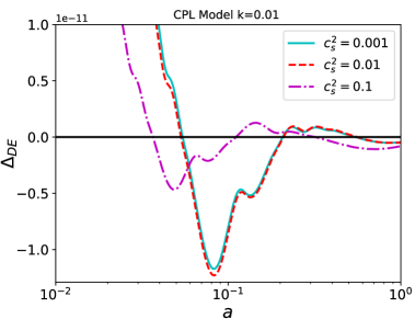
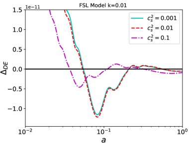
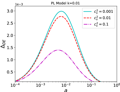
Figure 2: Clustering of dark energy at $k=0.01Mpc^{-1}$ affected by corresponding sound speed. Upper left panel indicates $\Delta_{\rm DE}$ for the CPL, upper right panel corresponds to $\Delta_{\rm DE}$ for the FSL, while lower panel is for $\Delta_{\rm DE}$ of the PL dark energy model. For PL model, clustering adopts only positive value associating with over-density while for CPL and FSL, we find negative and positive value of generalized density contrast. At the early epoch the value of clustering goes to its initial conditions. We take best fit values for free parameters determined by combining SNIa+ BAO+ HST+$Planck$ TT+LSS data sets.

4.  Structure Formation in DDE II: Clustering of Cold Dynamical Dark Energy

An important feature of dynamical dark energy is spatial perturbation, providing an independent key to investigate the nature of dark energy from equation of state and sound speed. The sound speed carries information about internal degree of freedom and low sound speed enhances the spatial variation of dark energy, giving rise to inhomogeneities or clusters. Clustering is a benchmark of dark energy perturbation which can affect on matter power spectrum and large scale clustering. It is investigated that a void on matter was seen to produce by local DDE overdensity and suggested DDE clustering might be relevant strong when matter perturbation goes non-linear [80]. In order to have considerable effect on matter power spectrum due to clustering of a typical dark energy, two necessity conditions should be satisfied [39]: dark energy equation of state must deviate from $-1$. All perturbations vanish as $1+w\rightarrow 0$, regardless of $c_{a}^{2}$. Secondly, the sound horizon $c_{s}H^{-1}$ of dark energy perturbation must be well within the Hubble scale that required $c_{s}^{2}\ll 1$ which considered as Cold Dark Energy (CDE).

Exact value of $c_{a}^{2}$ is hard to determine and degeneracy with other parameters come into play. In general case, sound speed is defined by:

$$c_{s}^{2}\equiv\frac{\delta P}{\delta\rho}=c_{s}^{2(A)}+c_{s}^{2(NA)}.$$ (4.1)

where adiabatic sound speed, $c_{s}^{2(A)}$, is purely determine by equation of state:

$$c_{s}^{2(A)}\equiv\dfrac{p\prime}{\rho\prime}=w_{\rm DE}-\dfrac{w\prime_{\rm DE}}{3{\mathcal{H}}(1+w_{\rm DE})}$$ (4.2)

where prime denote derivatives with respect to conformal time and $\mathcal{H}$ is the Hubble constant with respect to conformal time. Also $c_{s}^{2(NA)}$ represents non-adiabatic term. In general case, the pressure may depend on internal degree of freedom of the underlying fluid.

Supposing the dark energy behaves strictly as adiabatic fluid, consequently, sound speed is mainly affected by adiabatic term. For $c_{s}^{2}<0$, instability appears and to resolve this discrepancy, one can consider some classes of dynamical dark energy including other components which effectively causes to have $w_{eff}>0$ [81]. Another approach is supposing the non-adiabatic term in Eq. (4.1) to be survived.

In order to have stable clustering, the sound speed should adopt in the range of very small value to unity. Here in this paper we take $c_{s}^{2}=0.1$, $c_{s}^{2}=0.01$ and $c_{s}^{2}=0.001$ for clustering of dark energy at large scale $k=0.01h/Mpc$. In Fig. 2, we illustrate clustering of dark energy models as a function of scale factor for $k=0.01h/Mpc$ for various values of sound speed.

5.  Data Analysis I: Number of local maxima peaks

One of our aims is finding a proper way to distinguish between different DDE models. Many measures have been proposed ranging from geometrical and topological approaches to classical aspects [40, 41, 42, 82, 83, 84]. For example four minkowski functionals of morphological properties used of large scale structure were used to distinguish modified gravity models from general relativity [84]. Similarly, one can apply method base on cluster number counts method and number density of peaks trough to discriminate between models of DDE. To this end, we need to determine various order of for 2 dimensional field, given by:

$$\sigma^{2}_{m}\equiv\langle\triangledown^{m}\delta_{T}\triangledown^{m}\delta_{T}\rangle=\frac{1}{2\pi}\int dkk^{2m}P_{TT}(|k|)W^{2}(kR).$$ (5.1)

Hence $P_{TT}(k)$ is the power spectrum and $W$ stands for any smoothing function and $R$ is the smoothing scale. These parameter for a full sky CMB map are:

$$\sigma^{2}_{m}\equiv\sum_{\ell}\frac{(2\ell+1)}{4\pi}[\ell(\ell+1)]^{m}C_{\ell}^{TT}W_{\ell}^{2},$$ (5.2)

$C_{\ell}^{TT}$ represent the power spectrum for the full sky. $W_{\ell}$ is smoothing kernel associated with beam transfer function which is written by: $W_{\ell}=\exp(-\theta_{\rm beam}\ell(\ell+1)/2)$ and $\theta_{\rm beam}=\theta_{\rm FWHM}/\sqrt{8\ln(2)}$ [85, 86, 87]. In the flat sky approximation one can write:

$$\frac{\ell(\ell+1)C_{\ell}^{TT}}{2\pi}\backsim\frac{(360)^{2}}{2\pi}|k|^{2}P_{TT}(k).$$ (5.3)

By imposing the condition to have peaks above a given threshold, we find that:

$$\langle n_{p}(\vartheta;r)\rangle = \langle\Theta(\delta_{T}-\vartheta\sigma_{0})\delta_{D}(\eta_{\phi})\delta_{D}(\eta_{\phi})|{\rm Det}\xi|\rangle$$ (5.4)

$$= \int_{\rm conditions}\textit{P}(A_{\mu}|\delta_{T}\geqslant\vartheta\sigma_{0};\eta_{\phi}=\eta_{\phi}=0)|{\rm Det}\xi|dA_{\mu},$$

where $\Theta$ is the unit step function. The subscript "conditions" represents additional considerations for having local maxima. The number density of peaks for a purely homogeneous Gaussian CMB map in the rang of $[\vartheta,\vartheta+d\vartheta]$ becomes[85]:

$$n_{p}(\vartheta)=\frac{N_{\rm pix,tot}}{(2\pi)^{3/2}\gamma^{2}}e^{\frac{-\vartheta^{2}}{2}}G(\Gamma,\Gamma\vartheta),$$ (5.5)

where

$$G(\Gamma,\Gamma\vartheta) = (\Gamma^{2}\vartheta^{2}-\Gamma^{2})\left\{1-\frac{1}{2}{\rm erfc}\left[\frac{\Gamma\vartheta}{\sqrt{2(1-\Gamma^{2})}}\right]\right\}+\Gamma\vartheta(1-\Gamma^{2})\frac{\exp\left({-\frac{\Gamma^{2}\vartheta^{2}}{2(1-\Gamma^{2})}}\right)}{\sqrt{2\pi(1-\Gamma^{2})}}$$ (5.6)

$$+\frac{\exp\left({-\frac{\Gamma^{2}\vartheta^{2}}{3-2\Gamma^{2}}}\right)}{\sqrt{3-2\Gamma^{2}}}\left\{1-\frac{1}{2}{\rm erfc}\left[\frac{\Gamma\vartheta}{\sqrt{2(1-\Gamma^{2})(3-2\Gamma^{2})}}\right]\right\}.$$

Hence erfc(:) is the standard complementary error function, and the parameters $\Gamma$ and $\gamma$ are defined as $\Gamma\equiv\frac{\sigma_{1}^{2}}{\sigma_{0}\sigma_{1}}$ and $\gamma\equiv\sqrt{2}\frac{\sigma_{1}}{\sigma_{2}}$. Also $N_{\rm pix,tot}$ is the total number of pixel in a given map. Fig. 3 depicts the theoretical prediction of number density of peaks at a given threshold for three DDE models and cosmological constant. One can use local extrema for high negative or for high positive thresholds where the sensitivity of measure with respect to various models is reasonable.

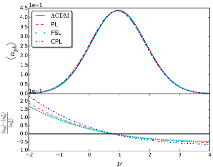
Figure 3: The number density of peaks for full sky CMB map in the presence of dynamical dark energy models. We consider the best fit values for free parameters of models from joint analysis SNIa+BAO+HST+$Planck$ TT+LSS.

6.  Data Analysis II: Observational constraints

In the current section, we will rely on the most recent observational data sets to revisit the observational consistency of underlying dynamical dark energy models explained in section 2. Accordingly, we will find the best fit values for associated free parameters in order to assess not only the impact of model at the background level but also to determine the clustering contribution of dark energy. Generally, following observables are utilized for further evaluation:
Geometric methods including various cosmological distance measures and dynamical methods which is mainly determined by Hubble parameter. Mentioned probes are mostly known as background contributions and to find more accurate identification, we can go beyond zero-order approximation and relying on higher order represented by evolution of perturbations. To this end, linear growth of density perturbations will be exploited to constrain free parameters of the models. We also examine evolution of gravitational potential, causing to Integrated Sachs-Wolfe (ISW) effect and also matter power spectrum and $f\sigma_{8}$ of models obtained. We will compute CMB power spectrum in the presence of DDE model neglecting the contribution of DDE clustering. Additional probes such as cross-correlation of CMB and large scale structures and Weak lensing will be left for future researches. In this paper we take into account the background expansion indicators such as distance modulus of Supernovae Type Ia and the Hubble parameter, Baryon acoustic oscillations (BAO), full sky CMB and $f\sigma_{8}$ data as flowing, our parameter space is:

$$\{\mathcal{P}\}\equiv\left\{\Omega_{\rm b}h^{2},\Omega_{\rm c}h^{2},\Theta,\tau,w_{0},w_{1},\alpha,n_{s},\ln\left[10^{10}\mathcal{A}_{s}\right]\right\}.$$ (6.1)

Hence, $\Omega_{\rm b}h^{2}$ and $\Omega_{\rm c}h^{2}$ are the physical baryon and cold dark matter densities, $\Theta$ is the ratio (multiplied by 100) of the sound horizon to angular diameter distance at decoupling, $\tau$ is the optical depth to re-ionization, $w_{0}$ and $w_{1}$ and $\alpha$ are free parameters of dark energy equation of states, $n_{s}$ is the scalar spectral index and $\mathcal{A}_{s}$ is defined as the amplitude of the initial power spectrum. The pivot scale of the initial scalar power spectrum we used here is $k_{p}=0.05Mpc^{-1}$ and we have assumed purely adiabatic initial condition. We have also supposed our Universe is flat, so $\Omega_{tot}=\Omega_{\rm c}+\Omega_{\rm b}+\Omega_{\rm rad}+\Omega_{\rm DE}=1$. The priors for free parameters of models have been mentioned in Table 1.

Parameter	Prior	Shape of PDF
$\Omega_{tot}$	1.000	Fixed
$\Omega_{b}h^{2}$	$[0.005-0.100]$	Top-Hat
$\Omega_{c}h^{2}$	$[0.001-0.990]$	Top-Hat
$\alpha$	$[0.00-0.20]$	Top-Hat
$w_{0}$	$[-1.2--0.9]$	Top-Hat
$w_{1}$	$[-0.2-0.2]$	Top-Hat
$H_{0}$	$[40.0-100.0]$	Top-Hat
$\tau$	$[0.01-0.80]$	Top-Hat
$n_{s}$	$[0.800-1.200]$	Top-Hat
$\ln(10^{10}\mathcal{A}_{s})$	$[2.000-4.000]$	Top-Hat

Table 1: Priors on parameter space, used in the posterior analysis.

6.1.  Luminosity distance

Type-Ia supernovae (SNIa) are among the most important probes of the Universe expansion and the main evidence for accelerating expansion epoch [1, 2]. Supernovae are considered as "standardizable candles" providing a measure for determining luminosity distance as a function of redshift. SNIa is categorized in cataclysmic variable stars which are created due to explosion of a white dwarf star and therefore its thermonuclear explosion is well known. Some of most important surveys of SNIa are: Higher-Z Team [88, 89], the Supernova Legacy Survey (SNLS) [90, 91, 92, 93], the ESSENCE [94, 95], the Nearby Supernova Factory (NSF) [96, 97], the Carnegie Supernova Project (CSP) [98, 99], the Lick Observatory Supernova Search (LOSS) [100, 101], the Sloan Digital Sky Survey (SDSS) SN Survey [102, 103], Union2.1 SNIa dataset [104, 105]. Recently Joint Light-curve Analysis (JLA) catalogue was produced from SNLS and SDSS SNIa compilation [106]. In this paper we consider SNIa observation data sets using JLA dataset including 740 SNIa in the redshift range of $z\in[0.01,1.30]$ [106].

However, the absolute luminosity of SNIa is considered uncertain and is marginalized out, which also removes any constraints on $H_{0}$. On the other hand, SNIa observations include low redshift data and effectively cover late-time expansion. So it could provide good constraints on models parameters. In practice direct observation of SNIa is given by corresponding distance modulus:

$$\mu(z;\{\mathcal{P}\})\equiv m-M=5\log\left({\frac{{{d_{L}}(z;\{\mathcal{P}\})}}{{\rm{Mpc}}}}\right)+25,$$ (6.2)

where $m$ and $M$ are apparent and absolute magnitude, respectively. For the spatially flat universe the luminosity distance defined in above equation reads as:

$${d_{L}}(z;\{\mathcal{P}\})=\frac{c}{{{H_{0}}}}(1+z)\mathop{\int}_{0}^{z}\frac{dz^{\prime}}{\mathcal{H}(z^{\prime};\{\mathcal{P}\})},$$ (6.3)

here $\mathcal{H}\equiv H/H_{0}$ and $H$ is Hubble parameter. In order to compare observational data set which predicted by model we utilize likelihood function with following $\chi^{2}$ form:

$$\chi^{2}_{SNIa}\equiv\Delta\mu^{{\dagger}}\cdot\mathcal{C}^{-1}_{SNIa}\cdot\Delta\mu,$$ (6.4)

where $\Delta\mu\equiv\mu_{obs}(z)-\mu(z;\{\Theta\})$ and $\mathcal{C}_{SNIa}$ is covariance matrix of SNIa data sets. $\mu_{obs}(z)$ is observed distance modulus for a SNIa located at redshift $z$. Marginalizing over $H_{0}$ as a nuisance parameter yields [107, 108]

$$\chi^{2}_{SNIa}=\mathcal{M}^{{\dagger}}\cdot\mathcal{C}_{SNIa}^{-1}\cdot\mathcal{M}+\mathcal{A}_{SNIa}+\mathcal{B}_{SNIa},$$ (6.5)

where $\mathcal{M}\equiv\mu_{obs}(z)-25-5\log_{10}[H_{0}d_{L}(z;\{\mathcal{P}\})/c]$, and

$$\mathcal{A} \equiv -\frac{\left[\sum_{i,j}\mathcal{M}(z_{i};\{\mathcal{P}\})\mathcal{C}^{-1}_{SNIa}(z_{i},z_{j})-\ln 10/5\right]^{2}}{\sum_{i,j}\mathcal{C}^{-1}_{SNIa}(z_{i},z_{j})},$$ (6.6)

$$\mathcal{B} \equiv -2\ln\left(\frac{\ln 10}{5}\sqrt{\frac{2\pi}{\sum_{i,j}\mathcal{C}^{-1}_{SNIa}(z_{i},z_{j})}}\right).$$ (6.7)

The observed distance modulus and the relevant covariance matrix can be found on the website [109, 110].

6.2.  Hubble constant

CMB includes mostly physics at the epoch of recombination, and so provides only weak direct constraints about low-redshift quantities through the integrated Sachs-Wolfe effect and CMB lensing. The CMB-inferred constraints on the local expansion rate $H_{0}$ are model dependent, and this makes the comparison to direct measurements interesting, since any mismatch could be evidence of new physics. Subsequently, we use Hubble constant measurement from Hubble Space Telescope (HST) $(H=73.8\pm 2.4kms^{-1}Mpc^{-1})$ with flat prior [111].

6.3.  Baryon Acoustic Oscillations

Baryon acoustic oscillations (BAO) are the imprint of oscillations produced in the baryon-photon plasma on the matter power spectrum. It reveals a standard ruler, but it is calibrated to the CMB-determined sound horizon at the end of the decoupling. The characteristic scale of this pattern is 152 Mpc in comoving scale. On this scale, matter fluctuations experience almost their linear regime. BAO criterion is almost sensitive to the dark energy and matter densities. Therefore, adding BAO prior in our analysis enables to reduce some degeneracies on cosmological parameters, especially for $\Omega_{c}h^{2}$ and $H_{0}$. The BAO data can be applied to measure both the angular diameter distance $D_{A}(z;\{\mathcal{P}\})$, and the expansion rate of the Universe $H(z;\{\mathcal{P}\})$. The combination of mentioned quantities is defined by [107]:

$$D_{V}(z;\{\mathcal{P}\})=\left[(1+z)^{2}D_{A}^{2}(z;\{\mathcal{P}\})\frac{cz}{H(z;\{\mathcal{P}\})}\right]^{1/3},$$ (6.8)

where $D_{V}(z;\{\mathcal{P}\})$ is volume-distance. The distance ratio in the context of BAO criterion is defined by:

$$d_{BAO}(z;\{\mathcal{P}\})\equiv\frac{r_{s}(z;\{\mathcal{P}\})}{D_{V}(z;\{\mathcal{P}\})}.$$ (6.9)

Hence, $r_{s}(z;\{\mathcal{P}\})$ is the comoving sound horizon. BAO observations contain 6 measurements from redshift interval, $z\in[0.1,0.7]$. In this paper, we use 6 measurements of BAO indicator including Sloan Digital Sky Survey (SDSS) data release 7 (DR7) [112], SDSS-III Baryon Oscillation Spectroscopic Survey (BOSS) [113], WiggleZ survey [114] and 6dFGS survey [115]. In Table 2 we report the observed values for BAO.

Redshift	Data Set	$d_{obs}$	Ref.
0.10	6dFGS	$0.336\pm 0.015$	[115]
0.35	SDSS-DR7-rec	$0.113\pm 0.002$	[112]
0.57	SDSS-DR9-rec	$0.073\pm 0.001$	[113]
0.44	WiggleZ	$0.0916\pm 0.0071$	[114]
0.60	WiggleZ	$0.0726\pm 0.0034$	[114]
0.73	WiggleZ	$0.0592\pm 0.0032$	[114]

Table 2: Observed data for BAO [hinshaw12].

The $d_{obs}(z)$ is reported in Table 2. The $\chi^{2}_{BAO}$ is defined by

$$\chi^{2}_{BAO}\equiv\Delta d^{{\dagger}}\cdot{\mathcal{C}}^{-1}_{BAO}\cdot\Delta d\,.$$ (6.10)

here $\Delta d(z;\{\mathcal{P}\})\equiv d_{obs}(z)-d_{BAO}(z;\{\mathcal{P}\})$, and inverse of covariance matrix, ${\mathcal{C}}^{-1}_{BAO}$, is [116]:

$${\mathcal{C}}^{-1}_{BAO}=\left(\begin{array}[]{rrrrrr}4444.4&0&0&0&0&0\\ 0&34.602&0&0&0&0\\ 0&0&20.661157&0&0&0\\ 0&0&0&24532.1&-25137.7&12099.1\\ 0&0&0&-25137.7&134598.4&-64783.9\\ 0&0&0&12099.1&-64783.9&128837.6\\ \end{array}\right).$$ (6.17)

6.4.  CMB observations

The CMB data alone is not able to put constraint on free parameters of dark energy models well. Because the main effects of dark energy constraint in the CMB anisotropy spectrum come from an angular diameter distance to the decoupling epoch $z\simeq 1100$ and the late integrated Sachs-Wolfe (ISW) effect. The late ISW effect cannot be accurately measured currently, therefore, only important information for constraint dark energy in the CMB data actually comes from the angular diameter distance to the last scattering surface However, if we consider clustering of DDE, one can expect to get non-trivial behavior and it needs to modify Boltzmann code to compute evolution of perturbations. In this work we focus on models which mainly affect the expansion history. To include all the aspects of models in cosmic evolution we use full CMB data from $Planck$ mission. In this part we use observed CMB power spectrum. The chi-square for this observation is:

$$\chi^{2}_{CMB-power}=\Delta C^{{\dagger}}\cdot\mathcal{M}^{-1}\cdot\Delta C,$$ (6.18)

here $\Delta C_{\ell}\equiv C_{\ell}^{obs}-C_{\ell}(\{\mathcal{P}\})$ and $\mathcal{M}$ is covariance matrix for CMB power spectrum. We also utilize CMB lensing from SMICA pipeline of $Planck$ 2015. To compute CMB power spectrum for our model, we modify Boltzmann code CAMB [117].

6.5.  $f\sigma_{8}$ observations

Using the amplitude of over-density at the comoving $8h^{-1}\rm Mpc$ scale and in order to obtain constraints from RSD measurements, The following quantity introduced as:

$$y(z)\equiv f(z)\sigma_{8}(z).$$ (6.19)

Throughout this paper we use most recent observational data sets based on SDSS-III, SDSS-II, DR7, VIPERS, RSD projects provided for $f(a)\sigma_{8}(a)$ to check the performance of DDE models (see [118, 119] which collected some points for $f\sigma_{8}$ at different redshifts and references therein).

Finally the total value of chi-square reads as:

$$\chi^{2}=\chi^{2}_{SNIa}+\chi^{2}_{BAO}+\chi^{2}_{HST}+\chi^{2}_{CMB}+\chi^{2}_{f\sigma_{8}}.$$ (6.20)

We utilize publicly available cosmological Markov Chain Monte Carlo code CosmoMC [120] to find a global fitting on the cosmological parameters in models. For CMB part we combine CAMB with CosmoMC. To take into account the rest of observational quantities, we write our code in python.

Parameter	PL	CPL	FSL
$\Omega_{b}h^{2}$	$0.02217\pm 0.00015$	$0.02218\pm 0.00016$	$0.02214\pm 0.00015$
$\Omega_{\rm c}h^{2}$	$0.1195\pm 0.0013$	$0.1193^{+0.0014}_{-0.0017}$	$0.1190^{+0.0013}_{-0.0016}$
$\Omega_{\rm DE}$	$0.6862\pm 0.0078$	$0.688^{+0.010}_{-0.0079}$	$0.6893\pm 0.0078$
$\alpha$	$0.1013\pm 0.0031$	$-$	$-$
$w_{0}$	$-1.3799^{+0.0036}_{-0.0028}$	$-1.08045^{+0.00041}_{-0.00062}$	$-0.9994\pm 0.0076$
$w_{1}$	$-$	$-0.12190^{+0.00050}_{-0.00030}$	$-0.0082^{+0.0044}_{-0.0051}$
$H_{0}$	$67.36\pm 0.56$	$67.48^{+0.71}_{-0.57}$	$67.56\pm 0.54$
$\Theta_{\rm MC}$	$1.04090^{+0.00072}_{-0.00076}$	$1.04094^{+0.00085}_{-0.00089}$	$1.04099^{+0.00068}_{-0.00073}$
$\tau$	$0.0828^{+0.0021}_{-0.0030}$	$0.0832^{+0.0028}_{-0.0034}$	$0.0837^{+0.0036}_{-0.0042}$
$n_{s}$	$0.9665^{+0.0079}_{-0.0076}$	$0.9641^{+0.0068}_{-0.0070}$	$0.9659^{+0.0074}_{-0.0078}$
$\ln\left(10^{10}A_{s}\right)$	$3.1006\pm 0.0038$	$3.0992^{+0.0065}_{-0.0070}$	$3.1009\pm 0.0041$

Table 3: The best fit values at $1\sigma$ confidence interval for free parameters of models based on joint analysis of SNIa+BAO+HST+$Planck$ TT+ LSS.

7.  Results and Discussion

In this section we will present the results of observational constraints for the CPL, FSL and PL as DDE models with the following observational data sets: 740 SNIa from JLA catalogue, the Hubble parameter at present time form HST, 6 data points for BAO, full sky CMB temperature power spectrum from $Planck$ 2015, $f\sigma_{8}$ observations by SDSS-II, SDSS-III, DR7, VIPERS and RSD projects. Then, we discuss our result for the three DDE models .

CPL model:
Combining all observational data sets namely, SNIa+BAO+HST+$Planck$ TT+LSS leads to $w_{0}=-1.08045^{+0.00041}_{-0.00062}$ and $w_{1}=-0.12190^{+0.00050}_{-0.00030}$ at $1\sigma$ confidence interval. Table 3 present the other free cosmological parameters of the model. Figs. 4 and 5 illustrate marginalized posterior probability distribution and the contours for the various parameters, receptively.

FSL model:
The best fit parameter of this model for the joint analysis of SNIa+BAO+HST+$Planck$ TT+LSS observation are: $w_{0}=-0.9994\pm 0.0076$ and $w_{1}=-0.0082^{+0.0044}_{-0.0051}$ at $1\sigma$ confidence interval. The rest of the parameters are given in table 3. Figs. 6 and 7 indicate the marginalized posterior probability distribution and contours for the various free parameters, respectively.

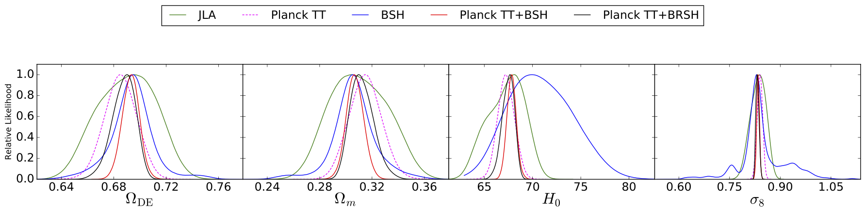
Figure 4: Marginalized posterior function for $\Omega_{\rm DE}$, $\Omega_{m}$, $H_{0}$ and $\sigma_{8}$ for CPL model. Solid green line corresponds to observational constraint by SNIa using JLA catalogue. Dashed pink line indicates constraint by $Planck$ TT data set. Blue line is devoted to joint analysis BAO+SNIa+HST (BSH). Red line is for joint analysis of $Planck$ TT+BSH. Combination of all observations is illustrated by thick solid black line.

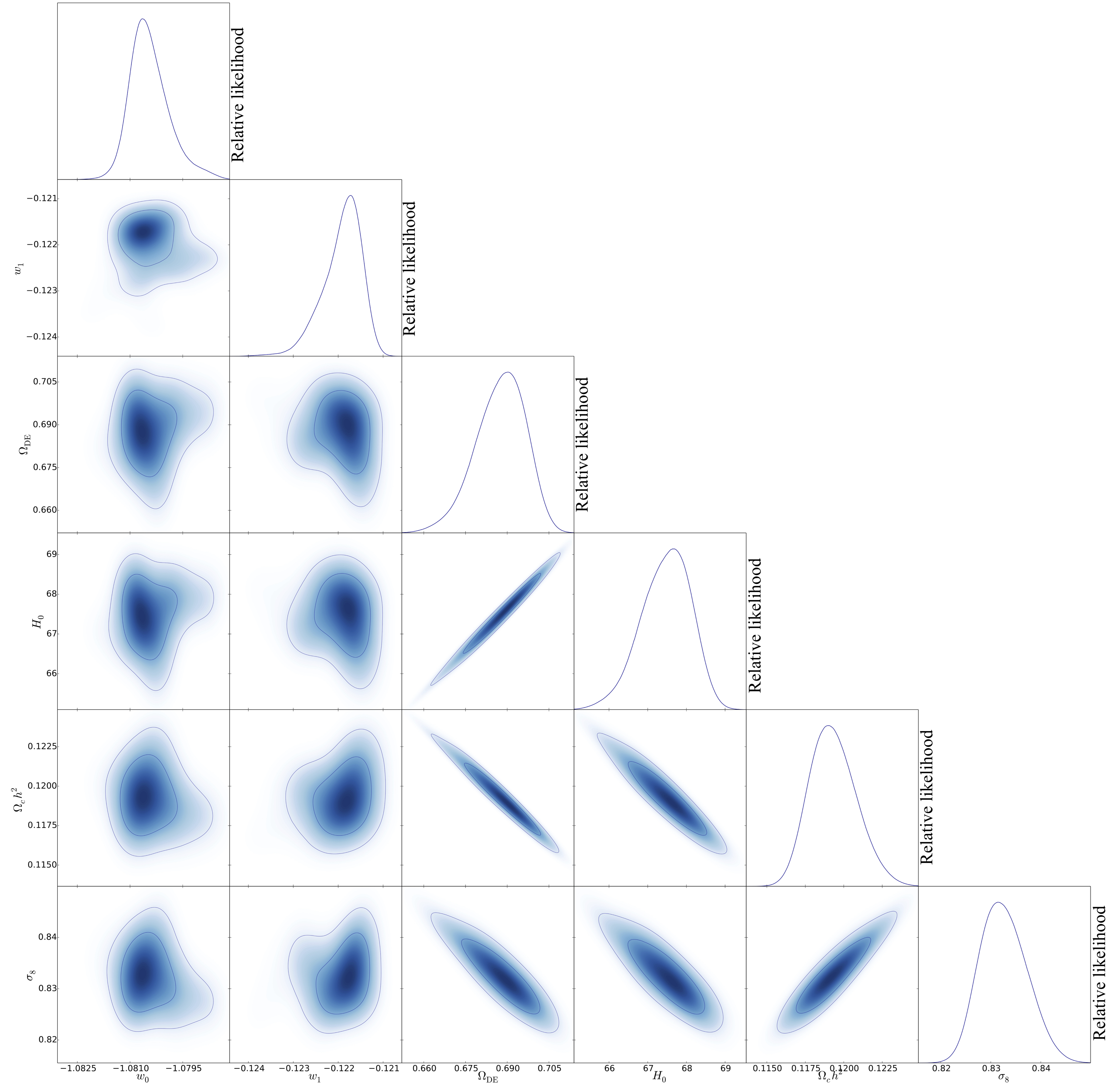
Figure 5: Measurement of various free parameters of CPL model from combination of SNIa+BAO+HST+$Planck$ TT+LSS observation. The 2-D regions with $1\sigma$ and $2\sigma$ level of confidences and corresponding 1-D marginalized posterior function are indicated in this figure.

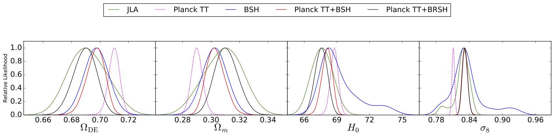
Figure 6: Marginalized posterior function for $\Omega_{\rm DE}$, $\Omega_{m}$, $H_{0}$ and $\sigma_{8}$ for FSL model. Solid green line corresponds to observational constraint by SNIa using JLA catalogue. Dashed pink line indicates constraint by $Planck$ TT data set. Blue line is devoted to joint analysis BAO+SNIa+HST (BSH).Red line is for joint analysis of $Planck$ TT+BSH. Combination of all observations is illustrated by thick solid black line.

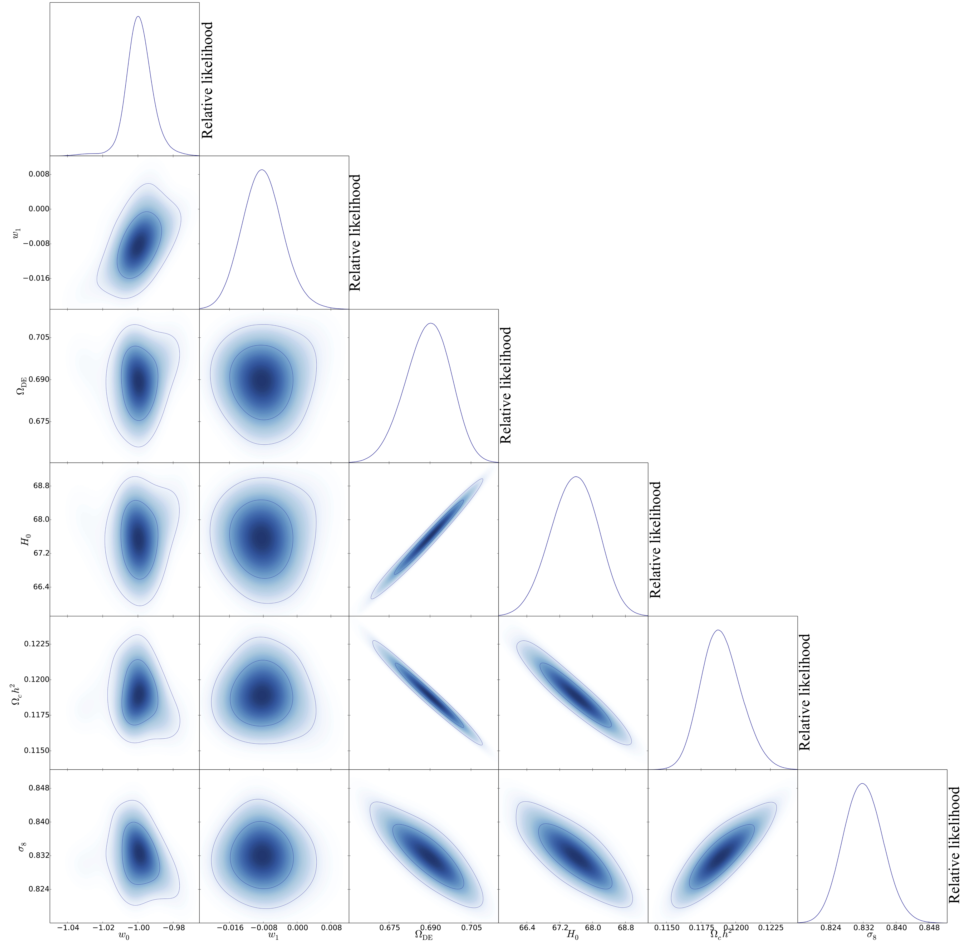
Figure 7: Measurement of various free parameters of FSL model from combination of SNIa+BAO+HST+$Planck$ TT+LSS observation. The 2-D regions with $1\sigma$ and $2\sigma$ level of confidences and corresponding 1-D marginalized posterior function are indicated in this figure.

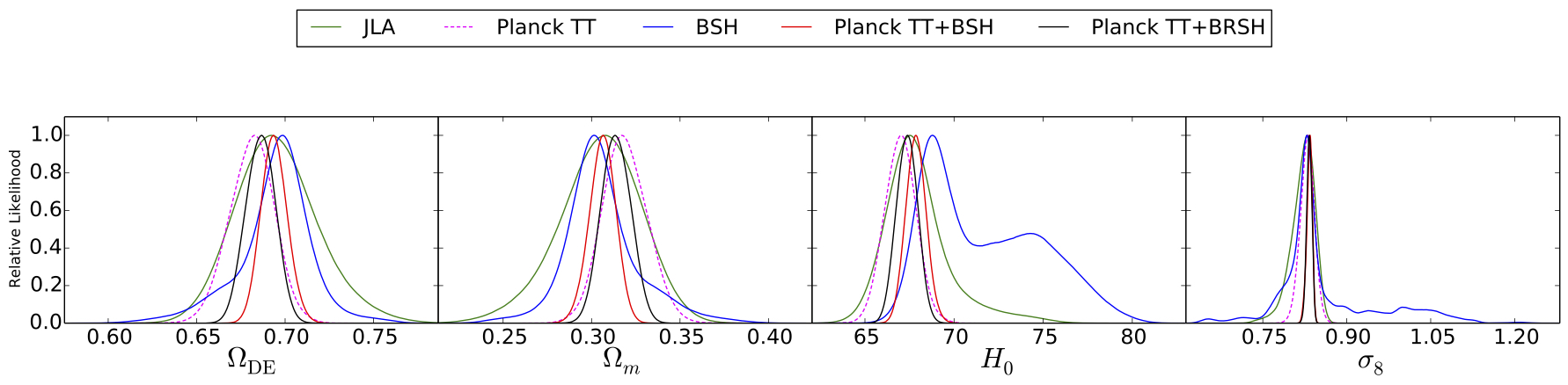
Figure 8: Marginalized posterior function for $\Omega_{\rm DE}$, $\Omega_{m}$, $H_{0}$ and $\sigma_{8}$ for PL model. Solid green line corresponds to observational constraint by SNIa using JLA catalogue. Dashed pink line indicates constraint by Planck TT data set. Blue line is devoted to joint analysis BAO+SNIa+HST (BSH). Red line is for joint analysis of $Planck$ TT+BSH. Combination of all observations is illustrated by thick solid black line.

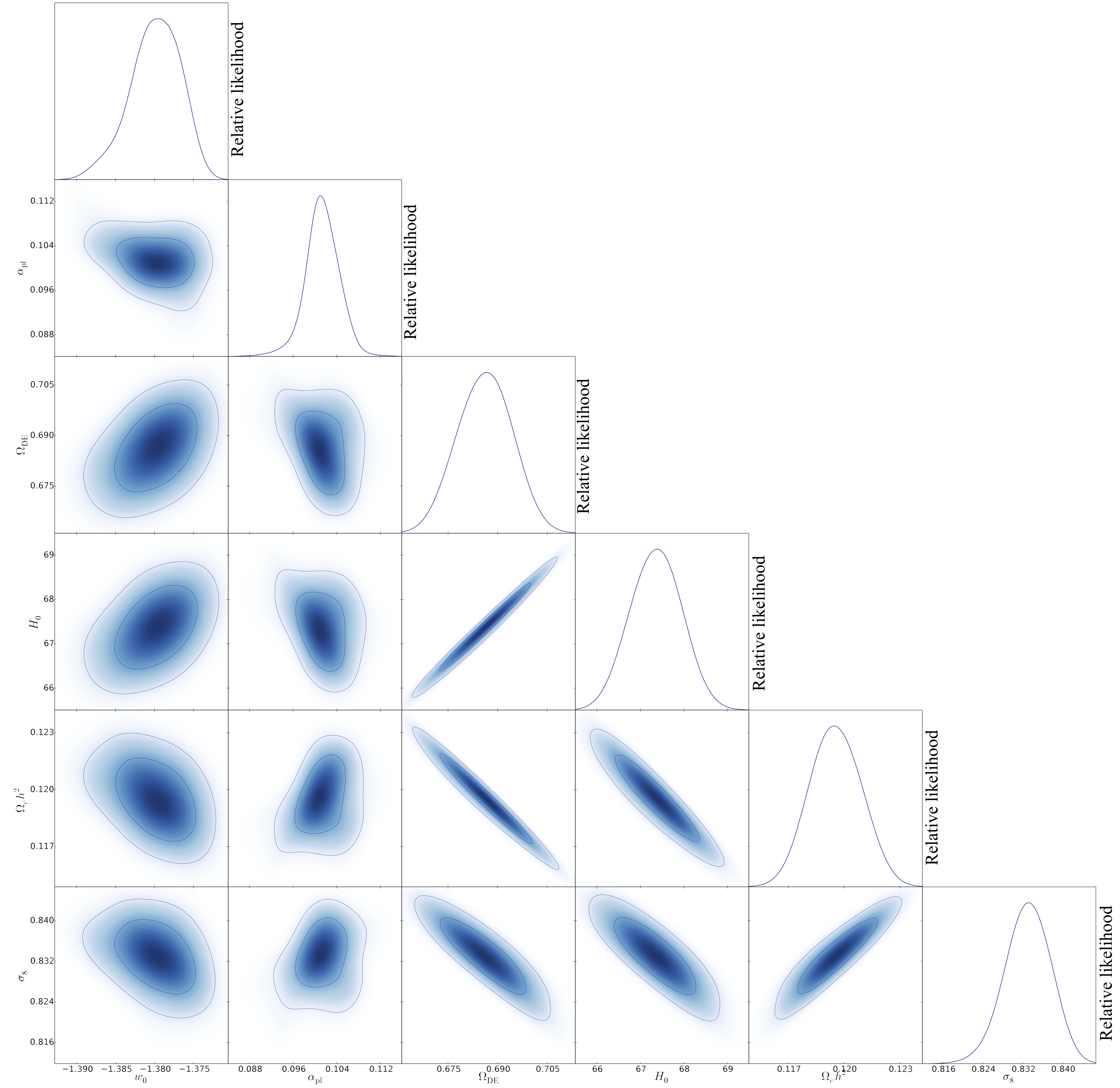
Figure 9: Measurement of various free parameters of PL model from combination of SNIa+BAO+HST+$Planck$ TT+LSS observation. The 2-D regions with $1\sigma$ and $2\sigma$ level of confidences and corresponding 1-D marginalized posterior function are indicated in this figure.

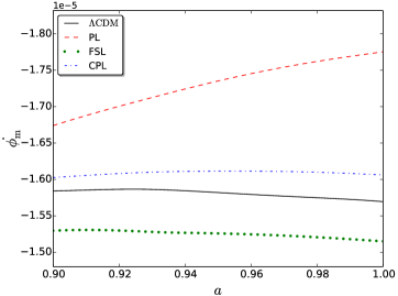
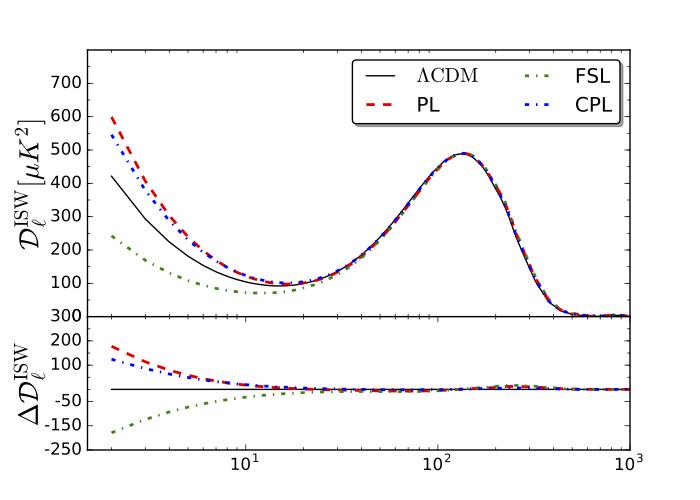
Figure 10: Left panel corresponds to evolution of time derivative of matter potential for various dark energy models versus scale factor in the linear regime. Right panel shows pure ISW effect as a function of $\ell$. The lower right panel illustrates difference of pure ISW power spectrum with $\lambda$CDM to make more obvious their deviations. We take best fit values for free parameters determined by combining SNIa+$Planck$ TT+ BAO+ HST+LSS data sets.

PL model:
The parameter of the power law model using the joint SNIa+BAO+HST+$Planck$ TT+LSS are $w_{0}=-1.3799^{+0.0036}_{-0.0028}$ and $\alpha=0.1013\pm 0.0031$ at $1\sigma$ confidence interval. Standard value for the standard cosmic parameters are given in table 3. Figs. 8 and 9 depict the marginalized posterior function and contours for various free parameters, respectively. The tension in $\sigma_{8}$ and $H_{0}$ as measured by Planck TT and late time observations, is almost alleviated in PL model.

It is also interesting to investigate the dynamical behavior of the matter potential which has the prominent role in producing the late ISW on the CMB anisotropy. Using the equation of state for the models compared to cosmological constant, we find that the associated matter potentials at linear regime for CPL and FSL follow closely the $\Lambda$CDM model. However PL model equation of state crossing $\Lambda$CDM and cause to achieve higher value for $\dot{\phi}_{m}$ all the time. The left panel of Fig. 10 indicates $\dot{\phi}_{m}$ as a function of scale factor for the best fit values given in table 3 by joint analysis. The right panel of Fig. 10 compute the ISW contribution to the CMB power spectrum for three DDE models. The lower part of right panel of Fig. 10 right panel shows deviation of late ISW contribution in the presence of CPL, FSL and PL models with respect to $\Lambda$CDM model .It demonstrate higher value for PL and lower value for FSL as expected from variation of potential. The full CMB temperature power spectrum $\mathcal{D}_{\ell}^{TT}$, with all source of the anisotropy included, is plotted in Fig. 11. The these DE models are consistent with data and not distinguishable from $\Lambda$CDM model with the given error bars. The Left panel Fig. 10 exhibits highest ISW contribution for PL compared to other DDE models, although the uncertainty due to cosmic variance cause that the best model is not measurable.

Fig. 12 shows the evolution of the matter density contrast $\Delta_{m}$ defined by Eq. (3.13) and the matter power spectrum computed for three DDE models. As illustrated in the left panel of Fig. 12, we find an enhancement in the matter growth for the PL model. This can be justified by comparing the values of $\Omega_{\rm DE}$ of the PL and $\Lambda$CDM models and by looking at the equation of state. The value of $\Omega_{\rm DE}$ for PL model is less than that of computed for $\Lambda$CDM model. The $\bar{w}_{\rm PL}$ behaves effectively similar to matter’s equation of state. On the other hand, there is suppression in the matter growth for the CPL model with the best fit parameters compared to $\Lambda$CDM model. For FSL, $\Delta_{m}$ is almost similar to the concordance model. The lower left panel of Fig. 12 represents the relative difference of observable density contrast to $\Lambda$CDM. The right panel of Fig. 12 indicates the matter power spectrum for various DDE models . We observe an excess of matter power spectrum for the PL model compared to the $\Lambda$CDM model especially at intermediate scales, namely $10^{-3}<k<2\times 10^{-1}$, with lower amount for the FSL and CPL models. This results is expected given the crossing behavior of the PL model. At early epoch, dark energy in PL contributes as cold dark matter leading to get more enhancement for structure formation. Also,the PL model exhibit strong clustering at lower value of scale factor and decrease with scale factor until present time. Such behavior may alter the cause for some of observational discrepancies such as missing satellite, which we postponed for next work trough N-body simulation of DDE models.

We turn to examine the $f\sigma_{8}(z)$ for three DDE models explained in this paper. As shown in Fig. 13, PL model has more consistency compared with other models. Our results demonstrates that, future observations with more precise accuracy enable us to discriminate PL model from $\Lambda$CDM-like models.

Now, we deal with examining relevant quantity coming from perturbation theory for our DDE models and we will compare them with $\Lambda$CDM model. As discussed in section 4, and plotted 2, the density contrast of dark energy component behaves differently as function of scale factor for various DDE models. In particular, the $\Delta_{DE}$ for PL is positive at all time with maximum of $\Delta_{PL}\simeq 10^{-3}$, while for other two models density contrast of dark energy has several crossing $\Delta_{DE}=0$ at various time depending on the model.the sound speed show how fast pressure perturbations propagate through the fluid. Higher values of $c_{s}^{2}$ leads to a decreased of clustering of dark energy for given initial perturbations. The plot of Fig. 2 also show the effect of sound speed on clustering of dark energy with different line style for DDE models. The CPL and FSL models show small clustering and exhibit dark energy void with deep valleys at the early universe.we also find that the FSL and CPL have a valley at early universe whose depth depends on sound speed. Reducing the sound speed increase the depth of valley and shifted it to late time.

The number density of peaks if we consider Gaussian random field for CMB in the presence of DDE models are indicated in Fig. 3. There are potential capability for discrimination of various DDE models for number density of peaks as a function of threshold at far from mean threshold. At $\nu=-2$ there is most separation between models, hence empty and dense regions are beneficial for discrimination of DDE models.

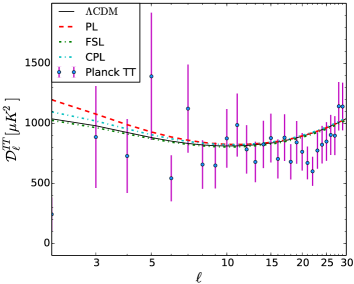
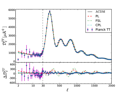
Figure 11: Left panel corresponds to temperature power spectrum of three DDE models at low $\ell$. Right panel indicates the TT power spectrum of CMB. Residuals with respect to $\Lambda$CDM model are shown in the lower panel. The error bars show at $1\sigma$ confidence interval. Best fit values for free parameters have been achieved by joint analysis of JLA+BAO+HST+CMB+LSS.

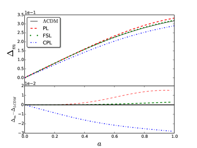
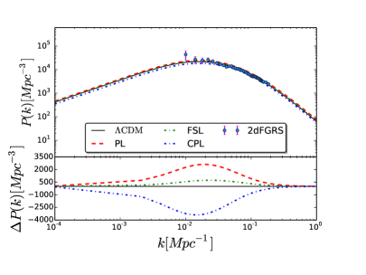
Figure 12: Left panel shows evolution of density contrast versus scale factor. The lower part of this panel represents difference between $\Delta_{m}$ and that of computed for $\Lambda$CDM model. The right panel corresponds to matter power spectrum of DDE models and for $\Lambda$CDM. Here to make more sense we show the 2dFGR data for matter power spectrum indicated by filled circle symbols. We compute the difference between $P(k)$ of DDE model an $\Lambda$CDM to make more sense in the lower part of this panel. Best fit values for free parameters have been determined by combining SNIa+ BAO+ HST+$Planck$ TT+LSS data sets.

In PL dynamical dark energy model, we have $\Omega_{\rm PL}(z_{lss})\approx 10^{-1}$ while $\Omega_{\rm{CPL},\rm{FSL}}(z_{lss})\approx 10^{-12}$. Therefore, one can not ignore the contribution of PL dark energy model at early era leading to some beneficial differences for upcoming data. Number of clusters expected by Euclid satellite enables to indicate detectable signal if EDE to be existed [39]. A robust indicator for searching the footprint of EDE is that: galaxy power spectrum amplitude at spatial scale greater than sound horizon is affected by dark energy clustering causing an enhancement which is sensitive to redshift evolution of net dark energy density (i.e. the equation of state) [35]. According 4, 6, 8 DDE models can improve $H_{0}$ tension, which Relative Likelihood of PL for Planck and SNIa completely cover each other and disappear the tension. Although CPL improved tension but there is separation between peak of two data set. FSL is not suitable model for $H_{0}$ tension.

$\rm{Model}$	$\chi^{2}_{min}$	$\Delta\rm{AIC}$	$\Delta\rm{BIC}$
$\Lambda$CDM	1629.69	0	0
$\rm{CPL}$	1631.57	3.88	18.077
$\rm{FSL}$	1629.87	2.18	17.007
$\rm{PL}$	1638.73	11.40	25.597

Table 4: The minimum value of $\chi^{2}$, $\Delta$AIC and $\Delta$BIC criteria for our models and $\Lambda$CDM when we use SNIa+ BAO+ HST+$Planck$ TT+LSS data sets.

There are standard technique for quantity comparison of different models with different parameter describing the same data sets. We will use some of these technique to compare the DDE models with each other and with $\Lambda$CDM model as a reference model. We need to other quantity in addition to determine $\chi^{2}$. It turns out that more degrees of freedom usually lead to better fit of the data with assumed model. However, there should be a penalty for adding to the of the model by introducing more parameters. In this work, we use $\chi^{2}$, AIC [121] and BIC [122] criteria for model comparison. AIC is defined by:

$${\rm AIC}=-2\ln{\mathcal{L}_{\rm{max}}}+2k,$$ (7.1)

and BIC [122] is given by:

$${\rm BIC}=-2\ln{\mathcal{L}_{\rm{max}}}+k\ln{N},$$ (7.2)

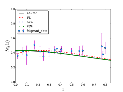
Figure 13: The model independent parameter for linear growth rate of cosmic structure in the present of dynamical dark energy models. Theoretical prediction indicated in this plot used the best fit values for free parameters achieved by joint analysis of JLA+BAO+HST+CMB+LSS.

In the above equations, $k$ is the number of free parameters. Note that BIC also depends on $N$, the number of observational data point carried out for implying observational constraints [123]. In practice, we reported these criteria for DDE models relative to $\Lambda$CDM , i.e $\Delta{\rm AIC}=\Delta\chi^{2}_{\rm{min}}+2\Delta g$ and $\Delta{\rm BIC}=\Delta\chi^{2}_{\rm{min}}+\Delta g\ln{N}$. Lower values of $\Delta$AIC and $\Delta$BIC, mean that the assumed model explain the data well. Table 4 report the $\Delta$AIC and $\Delta$BIC of the DDE models of our interest. The relevant quantities for mentioned purpose for our three models accompanying $\Lambda$CDM are reported in Table 4. Our results elucidate that our three dark energy models are supported by observations. We find that all considered models in this paper are worse than $\Lambda$CDM model but still are good models. Our results demonstrate that CPL and FSL are supported by observations with value of $\Delta$AIC$<10$. Note that with $\Lambda$CDM being reference model, the observation do not supported PL model strongly. However, the $\Lambda$CDM still gives a better description of the data.

8.  Conclusion

In this paper we consider three valuable dynamical dark energy models, namely, CPL, FSL and PL. We use most recent observational catalogues in order to confine the value of model free parameters. We implement joint light-curve analysis (JLA) for SNIa, baryon acoustic oscillation (BAO) from various surveys, Hubble parameter from HST-key project, Planck TT power spectrum and $f\sigma_{8}$ for large scale structure (LSS) observations. The joint analysis of JLA+BAO+HST+CMB+LSS, shows that $\Omega_{\rm DE}=0.6862\pm 0.0078$, $\alpha=0.1013\pm 0.0031$ and $w_{0}=-1.3799^{+0.0036}_{-0.0028}$ for Power-Law dynamical dark energy (DDE) model at $1\sigma$ confidence interval. The same observational constraints one optimal variance error for CPL model leads to $\Omega_{\rm DE}=0.6880^{+0.0100}_{-0.0079}$, $w_{0}=-1.08045^{+0.00041}_{-0.00062}$ and $w_{1}=-0.12190^{+0.00050}_{-0.00030}$. While for FSL model we find $\Omega_{\rm DE}=0.6893\pm 0.0078$, $w_{0}=-0.9994\pm 0.0076$ and $w_{1}=-0.0082^{+0.0044}_{-0.0051}$ at $1\sigma$ confidence limit. The tension in σ8 and H0 as measured by Planck TT and late time observations, is almost alleviated in PL model.

Since the variation of equation of state for PL is more than all DDE models considered in this paper, also due to more contribution of PL on cold matter at the early universe, namely $\Omega_{\rm PL}(z_{lss})\approx 10^{-1}$ while $\Omega_{\rm{CPL},\rm{FSL}}(z_{lss})\approx 10^{-12}$. Therefore, one can not ignore the contribution of PL dark energy model at early era leading to some beneficial differences for upcoming data. Structure formation gives us opportunity to discriminate between dynamical dark energy models. We find that growth of matter density in PL model is higher than other DDE models. For CPL, a considerable suppression for structure formation is achieved. The nature of dark energy can be investigated not only by equation of state but also through clustering and sound speed. We also examine the clustering of DDE model by modifying the relevant perturbation equations. The models show imaginary sound speed just PL exhibits positive value during period $0<a<0.4$ which cause instability in dark energy, so we consider $c_{s}^{2}=0.1$, $c_{s}^{2}=0.01$ and $c_{s}^{2}=0.001$ at large scale $k=0.01Mpc$. We obtained that, PL has positive clustering and grows fast during the early universe due to crossing behavior of equation of state and clod dark matter manner at the early time. The maximum of PL clustering is $\Delta_{PL}\simeq 10^{-3}$ and decreasing by increasing the sound speed. Hence, PL model has potential to produce more voids rather than other models [36] which is left for next work through the N-body simulation. The CPL and FSL exhibit small clustering at early time and density contrast of them have several crossing $\Delta_{DE}=0$ at various times. The CPL and FSL exhibit void of dark energy with deep and sharp valleys around $\Delta_{DE}\simeq-10^{-11}$ which depth of valleys are sensitive to sound speed and shifted to early time by increasing sound speed.

A geometrical measures namely the abundance of local maxima as a function of threshold for three DDE models elucidate that at far from mean threshold, it is potentially possible to look for a measure to discriminate different cosmological models.

The contribution of PL and CPL for late ISW are significant comparing to cosmological constant and FSL model. According Figs: 4, 8, 6, tension between HST and CMB for $H_{0}$ disappears for all models especially for PL model. The $f\sigma_{8}$ measure has been examined for our DDE models. Accordingly, future observations with more precise accuracy enable us to discriminate PL model from $\Lambda$CDM-like models. Not only, existence of early dark energy with 0.9 % density at %99 confidence level but also detect dark energy is cold rather than canonical %99 confidenc are possible with cluster survey of Euclid satellite in conjunction with CMB data [39]. Hence next generation data have sensitivity to discrimination between early dynamical dark energy and semi- $\Lambda$CDM models.

References

- [1] A. G. Riess et al. [Supernova Search Team Collaboration], Observational evidence from supernovae for an accelerating universe and a cosmological constant, Astron. J. 11 (1998) 1009 [astro-ph/9805201].
- [2] S. Perlmutter et al. [Supernova Cosmology Project Collaboration], Measurements of Omega and Lambda from 42 high redshift supernovae,’ Astrophys. J. 517 (1999) 565 [astro-ph/9812133].
- [3] C. Cheng and Q. G. Huang, An accurate determination of the Hubble constant from Baryon Acoustic Oscillation datasets, Sci. China Phys. Mech. Astron. 58 (2015) no.9, 599801 [astro-ph/1409.6119].
- [4] Beutler, Florian, et al. The 6dF Galaxy Survey: baryon acoustic oscillations and the local Hubble constant. Mon. Not. Roy. Astron. Soc. 416.4 (2011) 3017.
- [5] J. Martin, Everything You Always Wanted To Know About The Cosmological Constant Problem (But Were Afraid To Ask), Comptes Rendus Physique 13 (2012) 566 [astro-ph/1205.3365].
- [6] M. Kunz, The phenomenological approach to modeling the dark energy, Comptes Rendus Physique 13 (2012) 539 [astro-ph/1204.5482].
- [7] B. Moore, S. Ghigna, F. Governato, G. Lake, T. R. Quinn, J. Stadel and P. Tozzi, Dark matter substructure within galactic halos, Astrophys. J. 524 (1999) L19 [astro-ph/9907411].
- [8] A. A. Klypin, A. V. Kravtsov, O. Valenzuela and F. Prada, Where are the missing Galactic satellites?, Astrophys. J. 522 (1999) 82 [astro-ph/9901240].
- [9] J. F. Navarro, C. S. Frenk and S. D. M. White, The Structure of cold dark matter halos, Astrophys. J. 462 (1996) 563 [astro-ph/9508025].
- [10] W. J. G. de Blok,The Core-Cusp Problem, Adv. Astron. 2010, (2010) 789293.
- [11] F. Donato et al., A constant dark matter halo surface density in galaxies, Mon. Not. Roy. Astron. Soc. 397 (2009) 1169.
- [12] P. A. R. Ade et al. [Planck Collaboration], Planck 2015 results. XXIV. Cosmology from Sunyaev-Zeldovich cluster counts, Astron. Astrophys. 594 (2016) A24.
- [13] A. Y. Kamenshchik, U. Moschella and V. Pasquier, An Alternative to quintessence, Phys. Lett. B 511 (2001) 265 [gr-qc/0103004].
- [14] C. Armendariz-Picon, V. F. Mukhanov and P. J. Steinhardt, Essentials of k essence, Phys. Rev. D 63 (2001) 103510 [astro-ph/0006373].
- [15] R. R. Caldwell, A Phantom menace, Phys. Lett. B 545 (2002) 23 [astro-ph/9908168].
- [16] L. Amendola, Coupled quintessence, Phys. Rev. D 62 (2000) 043511 [astro-ph/9908023].
- [17] S. M. Carroll, V. Duvvuri, M. Trodden and M. S. Turner, Is cosmic speed - up due to new gravitational physics? Phys. Rev. D 70 (2004) 043528 [astro-ph/0306438].
- [18] S. Nojiri and S. D. Odintsov, Modified gravity with negative and positive powers of the curvature: Unification of the inflation and of the cosmic acceleration Phys. Rev. D 68 (2003) 123512 [hep-th/0307288].
- [19] L. Amendola, Scaling solutions in general nonminimal coupling theories Phys. Rev. D 60 (1999) 043501 [astro-ph/9904120].
- [20] J. P. Uzan, Cosmological scaling solutions of nonminimally coupled scalar fields Phys. Rev. D 59 (1999) 123510 [gr-qc/9903004].
- [21] E. J. Copeland, M. Sami and S. Tsujikawa, Dynamics of dark energy, Int. J. Mod. Phys. D 15 (2006) 1753 [hep-th/0603057].
- [22] S. Nojiri and S. D. Odintsov, Unified cosmic history in modified gravity: from F(R) theory to Lorentz non-invariant models, Phys. Rept. 505, 59 (2011) [gr-qc/1011.0544].
- [23] L. Amendola et al. [Euclid Theory Working Group Collaboration], Cosmology and fundamental physics with the Euclid satellite, Living Rev. Rel. 16 (2013) 6 [astro-ph/1206.1225].
- [24] P. Bull et al., Beyond CDM: Problems, solutions, and the road ahead, Phys. Dark Univ. 12 (2016) 56 [astro-ph/1512.05356].
- [25] G.W. Horndeski,Second-order scalar-tensor field equations in a four-dimensional space,” Int. J. Theor. Phys. 10 (1974) 363.
- [26] F. Könnig, H. Nersisyan, Y. Akrami, L. Amendola and M. Zumalacárregui, A spectre is haunting the cosmos: Quantum stability of massive gravity with ghosts, JHEP 1611 (2016) 118 [gr-qc/1605.08757].
- [27] M. C. Bento, O. Bertolami and A. A. Sen, Generalized Chaplygin gas, accelerated expansion and dark energy matter unification, Phys. Rev. D 66 (2002) 043507 [gr-qc/0202064].
- [28] B. Mostaghel, H. Moshafi and S. M. S. Movahed, Non-minimal Derivative Coupling Scalar Field and Bulk Viscous Dark Energy, Eur. Phys. J. C 77 (2017)541 [astro-ph/1611.08196].
- [29] N. Khosravi, Ensemble Average Theory of Gravity, Phys. Rev. D 94 (2016) 124035 [gr-qc/1606.01887].
- [30] Khosravi, Nima. Uber-Gravity and the Cosmological Constant Problem, [arXiv:1703.02052].
- [31] D. Huterer and M. S. Turner, Prospects for probing the dark energy via supernova distance measurements Phys. Rev. D 60 (1999) 081301 [astro-ph/9808133].
- [32] M. Sahlen, A. R. Liddle and D. Parkinson, Direct reconstruction of the quintessence potential Phys. Rev. D 72 (2005) 083511 [astro-ph/0506696].
- [33] R. Nair, S. Jhingan and D. Jain, Exploring scalar field dynamics with Gaussian processes JCAP 1401 (2014) 005. [astro-ph/1306.0606].
- [34] Holsclaw, Tracy, et al. Nonparametric reconstruction of the dark energy equation of state, Physical Review D 82.10 (2010) 103502 [astro-ph/1009.5443 ].
- [35] M. Takada, Can A Galaxy Redshift Survey Measure Dark Energy Clustering, Phys. Rev. D 74 (2006) 043505 [astro-ph/0606533].
- [36] S. Dutta and I. Maor, Voids of dark energy, Phys. Rev. D 75 (2007) 063507 [gr-qc/0612027].
- [37] Q. Wang, Z. and Fan, Simulation studies of dark energy clustering induced by the formation of dark matter halos, Phys. Rev. D 85 (2012) 023002.
- [38] Q. Wang, Z. and Fan, Dynamical evolution of quintessence dark energy in collapsing dark matter halos,Phys. Rev. D 79 (2009) 123012 [astro-ph/0906.3349].
- [39] S. A. Appleby, E. V. Linder and J. Weller, Cluster Probes of Dark Energy Clustering, Phys. Rev. D 88 (2013) 043526 [astro-ph/1305.6982].
- [40] B. Jain and A. Taylor, Cross-correlation tomography: measuring dark energy evolution with weak lensing, Phys. Rev. Lett. 91 (2003) 141302 [astro-ph/0306046].
- [41] A.N. Taylor, T.D. Kitching, D.J. Bacon, A.F. Heavens, Probing dark energy with the shear-ratio geometric test, Mon. Not. Roy. Astron. Soc. 374 (2007) 1377.
- [42] T.D. Kitching, A.N. Taylor, A.F. Heavens, Systematic effects on dark energy from 3D weak shear, Mon. Not. Roy. Astron. Soc. 389 (2008) 173.
- [43] V. Sahni, T. D. Saini, A. A. Starobinsky and U. Alam, Statefinder: A New geometrical diagnostic of dark energy JETP Lett. 77 (2003) 201 [astro-ph/0201498].
- [44] M. Arabsalmani and V. Sahni, The Statefinder hierarchy: An extended null diagnostic for concordance cosmology Phys. Rev. D 83 (2011) 043501 [astro-ph/1101.3436].
- [45] A. F. Heavens, T. D. Kitching, and L. Verde, On model selection forecasting, Dark Energy and modified gravity, Mon.Not.Roy.Astron.Soc.380 (2007) 1029 [astro-ph/0703191v2].
- [46] T. Abbott et al. [DES Collaboration], The dark energy survey, [astro-ph/0510346].
- [47] R. Laureijs et al., Euclid Definition Study Report, [arXiv:1606.00180] .
- [48] R. DeBoerr, R. David, et al. Australian SKA pathfinder: A high-dynamic range wide-field of view survey telescope. Proceedings of the IEEE 97.8 (2009) 1507.
- [49] P. Andre et al. [PRISM Collaboration], PRISM (Polarized Radiation Imaging and Spectroscopy Mission): A White Paper on the Ultimate Polarimetric Spectro-Imaging of the Microwave and Far-Infrared Sky, [astro-ph/1306.2259].
- [50] C. Armitage-Caplan, et al. COrE (Cosmic Origins Explorer) A White Paper, [ arXiv:1102.2181] .
- [51] T. Denkiewicz, Dynamical dark energy models with singularities in the view of the forthcoming results of the growth observations [arXiv:1511.04708]
- [52] R. R. Caldwell and E. V. Linder, The Limits of quintessence, Phys. Rev. Lett. 95 (2005) 141301 [astro-ph/0505494].
- [53] Brax, Philippe, and Patrick Valageas. Goldstone models of modified gravity, Phys. Rev. D 95.4 (2017) 043515.
- [54] M. Honda, N. Iizuka, A. Tanaka and S. Terashima, Exact Path Integral for 3D Higher Spin Gravity, Phys. Rev. D 95 (2017) 046016 [hep-th/1511.07546].
- [55] T. Koivisto and D. F. Mota, Dark energy anisotropic stress and large scale structure formation, Phys. Rev. D 73 (2006) 083502 [astro-ph/0512135].
- [56] B. A. Bassett, P. S. Corasaniti and M. Kunz, The Essence of quintessence and the cost of compression, Astrophys. J. 617 (2004) L1 [astro-ph/0407364].
- [57] M. Chevallier and D. Polarski, Accelerating universes with scaling dark matter, Int. J. Mod. Phys. D 10 (2001) 213 [gr-qc/0009008].
- [58] E. V. Linder, Exploring the expansion history of the universe, Phys. Rev. Lett. 90 (2003) 091301 [astro-ph/0208512].
- [59] J. Z. Ma and X. Zhang, Probing the dynamics of dark energy with novel parametrizations, Phys. Lett. B 699 (2011) 233 [astro-ph/1102.2671].
- [60] V. Salzano, Y. Wang, I. Sendra and R. Lazkoz, Linear dark energy equation of state revealed by supernovae, Mod. Phys. Lett. A 29 (2014) 1450008 [astro-ph/1211.1012].
- [61] C. J. Feng, X. Y. Shen, P. Li and X. Z. Li, A New Class of Parametrization for Dark Energy without Divergence, JCAP 1209 (2012) 023 [astro-ph/1206.0063].
- [62] S. Rahvar and M. S. Movahed, Power-law Parameterized Quintessence Model, Phys. Rev. D 75 (2007) 023512 [astro-ph/0604206].
- [63] W.H. Julian, On the effect of interstellar material on stellar non- circular velocities in disk galaxies, Astrophys. J. 148 (1967) 175.
- [64] C. P. Ma and E. Bertschinger, Cosmological perturbation theory in the synchronous and conformal Newtonian gauges, Astrophys. J. 455 (1995) 7 [astro-ph/9506072].
- [65] Sapone, Domenico, and Martin Kunz. Fingerprinting dark energy, Phys. Rev. D 80.8 (2009) 083519 [astro-ph/0909.0007].
- [66] A. Meiksin and M. WhiteThe growth of correlations in the matter power spectrum, Mon. Not. Roy. Astron. Soc. 308 (1999)1179.
- [67] A. Pouri, S. Basilakos and M. Plionis, Precision growth index using the clustering of cosmic structures and growth data, JCAP 1408 (2014) 042 [astro-ph/1402.0964].
- [68] C. P. Ma, R. R. Caldwell, P. Bode and L. M. Wang, The mass power spectrum in quintessence cosmological models, Astrophys. J. 521 (1999) L1 [astro-ph/9906174].
- [69] S. Dodelson, Modern Cosmology , Academic Press, New York (2008).
- [70] J.M. Bardeen, J.R. Bond, N. Kaiser, and A.S. Szalay,The statistics of peaks of Gaussian random fields, Astrophys. J. 304 (1986)15 .
- [71] P. A. R. Ade et al. [Planck Collaboration], Planck 2015 results. XIII. Cosmological parameters, Astron. Astrophys. 594 (2016) A13 [astro-ph/1502.01589].
- [72] Y. S. Song and W. J. Percival, Reconstructing the history of structure formation using Redshift Distortions, JCAP 0910 (2009) 004 [astro-ph0807.0810].
- [73] Kaiser, Nick. Clustering in real space and in redshift space, Mon. Not. Roy. Astron. Soc. 227.1 (1987) 1.
- [74] S. Nesseris, G. Pantazis and L. Perivolaropoulos, Tension and constraints on modified gravity parametrizations of from growth rate and Planck data, Phys. Rev. D 96 (2017) 023542 [astro-ph/1703.10538].
- [75] Weller, Jochen, and A. M. Lewis. Large-scale cosmic microwave background anisotropies and dark energy, Mon. Not. Roy. Astron. Soc. 346.3 (2003) 987.
- [76] R. K. Sachs and A. M. Wolfe, Perturbations of a cosmological model and angular variations of the microwave background, Astrophys. J. 147 (1967) 73.
- [77] W. Hu and N. Sugiyama, Anisotropies in the cosmic microwave background: An Analytic approach, Astrophys. J. 444 (1995) 489 [astro-ph/9407093].
- [78] Gold, Benjamin. Limits of dark energy measurements from correlations of CMB lensing, the integrated Sachs-Wolfe effect, and galaxy counts, Phys. Rev. D 71.6 (2005) 063522.
- [79] G. Olivares, F. Atrio-Barandela and D. Pavon, The Integrated Sachs-Wolfe Effect in Interacting Dark Energy Models, Phys. Rev. D 77 (2008) 103520 [astro-ph/0801.4517].
- [80] D. F. Mota, D. J. Shaw and J. Silk, On the Magnitude of Dark Energy Voids and Overdensities, Astrophys. J. 675 (2008) 29 [astro-ph/0709.2227].
- [81] P. Roland, D. Huterer, and Eric V. Linder. Measuring the speed of dark: detecting dark energy perturbations, Phys. Rev. D 81.10 (2010) 103513 [astro-ph/1002.1311].
- [82] C. Ling, Q. Wang, R. Li, B. Li, J. Wang and L. Gao, Distinguishing general relativity and gravity with the gravitational lensing Minkowski functionals, Phys. Rev. D 92 (2015) 064024 [astro-ph/1410.2734].
- [83] M. Shirasaki, T. Nishimichi, B. Li and Y. Higuchi, The imprint of f(R) gravity on weak gravitational lensing ? II. Information content in cosmic shear statistics, Mon. Not. Roy. Astron. Soc. 466 (2017) 2402 [astro-ph/1610.03600].
- [84] W. Fang, B. Li and G. B. Zhao, New Probe of Departures from General Relativity Using Minkowski Functionals, Phys. Rev. Lett. 118 (2017) 181301 [astro-ph/1704.02325].
- [85] Bond, J. R., and G. Efstathiou. The statistics of cosmic background radiation fluctuations, Mon. Not. Roy. Astron. Soc. 226 (1987) 655.
- [86] A. F. Heavens and R. K. Sheth, The correlation of peaks in the microwave background, Mon. Not. Roy. Astron. Soc. 310, 1062 (1999) [astro-ph/9904307].
- [87] C. Hikage, E. Komatsu and T. Matsubara, Primordial Non-Gaussianity and Analytical Formula for Minkowski Functionals of the Cosmic Microwave Background and Large-scale Structure, Astrophys. J. 653 (2006) 11 [astro-ph/0607284].
- [88] A. G. Riess et al. [Supernova Search Team], Type Ia supernova discoveries at z > 1 from the Hubble Space Telescope: Evidence for past deceleration and constraints on dark energy evolution, Astrophys. J. 607 (2004) 665 [astro-ph/0402512].
- [89] A. G. Riess et al., New Hubble Space Telescope Discoveries of Type Ia Supernovae at z>=1: Narrowing Constraints on the Early Behavior of Dark Energy, Astrophys. J. 659 (2007) 98 [astro-ph/0611572].
- [90] P. Astier et al. [SNLS Collaboration], The Supernova legacy survey: Measurement of omega(m), omega(lambda) and W from the first year data set, Astron. Astrophys. 447 (2006) 31 [astro-ph/0510447].
- [91] S. Baumont et al. [SNLS Collaboration], PHotometry Assisted Spectral Extraction (PHASE) and identification of SNLS supernovae, Astron. Astrophys. 491 (2008) 567 [astro-ph/0809.4407].
- [92] N. Regnault et al. [SNLS Collaboration], Photometric Calibration of the Supernova Legacy Survey Fields, Astron. Astrophys. 506 (2009) 999. [astro-ph/0908.3808].
- [93] J. Guy et al. [SNLS Collaboration], The Supernova Legacy Survey 3-year sample: Type Ia Supernovae photometric distances and cosmological constraints, Astron. Astrophys. 523 (2010) A7 [astro-ph/1010.4743].
- [94] G. Miknaitis et al., The ESSENCE Supernova Survey: Survey Optimization, Observations, and Supernova Photometry, Astrophys. J. 666 (2007) 674 [astro-ph/0701043].
- [95] W. M. Wood-Vasey et al. [ESSENCE Collaboration], Observational Constraints on the Nature of the Dark Energy: First Cosmological Results from the ESSENCE Supernova Survey, Astrophys. J. 666 (2007) 694 [astro-ph/0701041].
- [96] W. M. Wood-Vasey et al., The nearby supernova factory, New Astron. Rev. 48 (2004) 637 [astro-ph/0401513].
- [97] R. A. Scalzo et al., Nearby Supernova Factory Observations of SN 2007if: First Total Mass Measurement of a Super-Chandrasekhar-Mass Progenitor, Astrophys. J. 713 (2010) 1073 [arXiv:1003.2217 [astro-ph.CO]].
- [98] G. Folatelli et al., The Carnegie Supernova Project: Analysis of the First Sample of Low-Redshift Type-Ia Supernovae, Astron. J. 139 (2010) 120 [[astro-ph/0910.3317].
- [99] C. Contreras et al., The Carnegie Supernova Project: First Photometry Data Release of Low-Redshift Type Ia Supernovae, Astron. J. 139 (2010) 519 [astro-ph/0910.3330].
- [100] J. Leaman, W. Li, R. Chornock and A. V. Filippenko, Nearby Supernova Rates from the Lick Observatory Supernova Search. I. The Methods and Database, Mon. Not. Roy. Astron. Soc. 412 (2011) 1419 [astro-ph/1006.4611].
- [101] Li, Weidong, et al. Nearby supernova rates from the Lick Observatory Supernova Search–III. The rate–size relation, and the rates as a function of galaxy Hubble type and colour, Mon. Not. Roy. Astron. Soc. 412.3 (2011) 1473.
- [102] J. A. Holtzman et al. [SDSS Collaboration], The Sloan Digital Sky Survey-II Photometry and Supernova IA Light Curves from the 2005 Data, Astron. J. 136 (2008) 2306 [astro-ph/0908.4277].
- [103] R. Kessler et al., First-year Sloan Digital Sky Survey-II (SDSS-II) Supernova Results: Hubble Diagram and Cosmological Parameters, Astrophys. J. Suppl. 185 (2009) 32 [astro-ph/0908.4274].
- [104] N. Suzuki et al., The Hubble Space Telescope Cluster Supernova Survey: V. Improving the Dark Energy Constraints Above z>1 and Building an Early-Type-Hosted Supernova Sample, Astrophys. J. 746 (2012) 85 [astro-ph/1105.3470].
- [105] S. Cao and Z. H. Zhu, Cosmic equation of state from combined angular diameter distances: Does the tension with luminosity distances exist, Phys. Rev. D 90 (2014) 083006 [astro-ph/1410.6567].
- [106] M. Betoule et al. [SDSS Collaboration], Improved cosmological constraints from a joint analysis of the SDSS-II and SNLS supernova samples, Astron. Astrophys. 568 (2014) A22 [astro-ph/1401.4064].
- [107] P. A. R. Ade et al. [Planck Collaboration], Planck 2015 results. XIV. Dark energy and modified gravity, Astron. Astrophys. 594 (2016) A14 [astro-ph/1502.01590].
- [108] Z. Li, P. Wu and H. Yu, Examining the cosmic acceleration with the latest Union2 supernova data, Phys. Lett. B 695 (2011) 1.
- [109] http://supernova.lbl.gov/Union/
- [110] http://supernovae.in2p3.fr/sdss_snls_jla/ReadMe.html
- [111] Riess, Adam G., et al. A 3% solution: determination of the Hubble constant with the Hubble Space Telescope and Wide Field Camera 3, Astrophys. J. 730.2 (2011) 119.
- [112] N. Padmanabhan, X. Xu, D. J. Eisenstein, R. Scalzo, A. J. Cuesta, K. T. Mehta and E. Kazin, A 2 per cent distance to =0.35 by reconstructing baryon acoustic oscillations - I. Methods and application to the Sloan Digital Sky Survey, Mon. Not. Roy. Astron. Soc. 427 (2012) 2132.
- [113] L. Anderson et al., The clustering of galaxies in the SDSS-III Baryon Oscillation Spectroscopic Survey: Baryon Acoustic Oscillations in the Data Release 9 Spectroscopic Galaxy Sample, Mon. Not. Roy. Astron. Soc. 427 (2013) 3435.
- [114] C. Blake et al., The WiggleZ Dark Energy Survey: Joint measurements of the expansion and growth history at z < 1, Mon. Not. Roy. Astron. Soc. 425 (2012) 405.
- [115] F. Beutler et al., The 6dF Galaxy Survey: Baryon Acoustic Oscillations and the Local Hubble Constant, Mon. Not. Roy. Astron. Soc. 416 (2011) 3017.
- [116] G. Hinshaw et al. [WMAP Collaboration], Nine-Year Wilkinson Microwave Anisotropy Probe (WMAP) Observations: Cosmological Parameter Results, Astrophys. J. Suppl. 208 (2013) 19 [astro-ph/1212.5226].
- [117] A. Lewis, A. Challinor and A. Lasenby, Efficient computation of CMB anisotropies in closed FRW models, Astrophys. J. 538 (2000) 473 [astro-ph/9911177].
- [118] C. Q. Geng, C. C. Lee and L. Yin, Constraints on running vacuum model with and , JCAP 1708 (2017) 032 [astro-ph/1704.02136].
- [119] X. W. Duan, M. Zhou and T. J. Zhang, Testing consistency of general relativity with kinematic and dynamical probes, [astro-ph/1605.03947 ].
- [120] A. Lewis and S. Bridle, Cosmological parameters from CMB and other data: A Monte Carlo approach, Phys. Rev. D 66 (2002) 103511 [astro-ph/0205436].
- [121] Akaike, Hirotugu. A new look at the statistical model identification, IEEE transactions on automatic control 19.6 (1974) 716.
- [122] G. Schwarz, Estimating the dimension of a model. Ann. Stat. 6 (1978) 461.
- [123] Y. Y. Xu and X. Zhang, Comparison of dark energy models after Planck 2015, Eur. Phys. J. C 76 (2016) 588 [astro-ph/1607.06262].