Robust Continuous Co-Clustering

Abstract

Clustering consists on grouping together samples giving their similar properties. The problem of modeling simultaneously groups of samples and features is known as Co-Clustering. This paper introduces ROCCO - a Robust Continuous Co-Clustering algorithm. ROCCO is a scalable, hyperparameter-free, easy and ready to use algorithm to address Co-Clustering problems in practice over massive cross-domain datasets. It operates by learning a graph-based two-sided representation of the input matrix. The underlying proposed optimization problem is non-convex, which assures a flexible pool of solutions. Moreover, we prove that it can be solved with a near linear time complexity on the input size. An exhaustive large-scale experimental testbed conducted with both synthetic and real-world datasets demonstrates ROCCO’s properties in practice: (i) State-of-the-art performance in cross-domain real-world problems including Biomedicine and Text Mining; (ii) very low sensitivity to hyperparameter settings; (iii) robustness to noise and (iv) a linear empirical scalability in practice. These results highlight ROCCO as a powerful general-purpose co-clustering algorithm for cross-domain practitioners, regardless of their technical background.

1 Introduction

Clustering consists on grouping together objects (samples) giving their similar properties (features). However, in practical high-dimensional data mining problems, it is often observed that such groups actually share only a subset of such properties - representing a context (e.g. peak hour definition in Transportation [KMMCC16]). The problem of modeling simultaneously groups of samples and features is known as bi-clustering or Co-Clustering (CoC) [CAB17, BPP08]. It outputs a natural interpretability of their results through an explicit definition of a feature subspace (not necessarily exclusive) for each resulting cluster. This characteristic turns it interesting to apply in practice. Real-world examples range different domains, from Biomedicine [CAB17] to Text mining [Dhi01] or Marketing/Retail [HP99].

Similarly to one-sided clustering, existing solutions to the CoC problem typically suffer from (at least) one of the following issues:

• Scalability concerns the algorithm’s ability to address large-scale datasets while keeping a reasonable ratio runtime vs. input size. SAMBA [TSS02] is a notorious example of this issue by scaling its runtime exponentially on the feature space.

• Model or Hyperparameter Tuning: Since CoC is an unsupervised learning process, the choice of adequate hyperparameter values often requires human expertise and/or time-consuming processes. Convex Bi-ClusteRing Algorithm (COBRA [CAB17]) is one of the most recently proposed CoC methods and, like many of its predecessors, it is highly sensitive to its hyperparameter setting.

• Stability: Many algorithms are initialization-dependent, requiring the usage of heuristics that often incur on re-training models multiple times (e.g. $K$-Means ). Many CoC algorithms (e.g. Spectral Co-Clustering (SCC) [Dhi01]) have $K$-Means (i.e. KM) as a building block, inheriting this disadvantage.

• Noise (In)tolerance: Real-world datasets often contain highly noisy records, turning many clustering algorithms not directly usable in practice - especially when facing high noise vs. patterns ratios [MP16]. OP-Cluster [LW03] is an approach for CoC that evolves from a sequential pattern mining approach, requiring clusters to have a considerable support to be found.

This paper introduces ROCCO - a Robust Continuous Co-Clustering algorithm. ROCCO is a scalable, robust, easy and ready to use algorithm to address CoC problems in practice over massive - and possible noisy - cross-domain datasets. It operates by learning a graph-based two-sided representation of the input matrix with a good CoC structure. The underlying proposed optimization problem is non-convex - which assures a flexible pool of solutions. Moreover, we prove that it can be solved with an empirical linear time complexity on the input size.

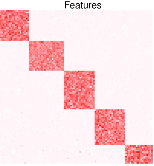
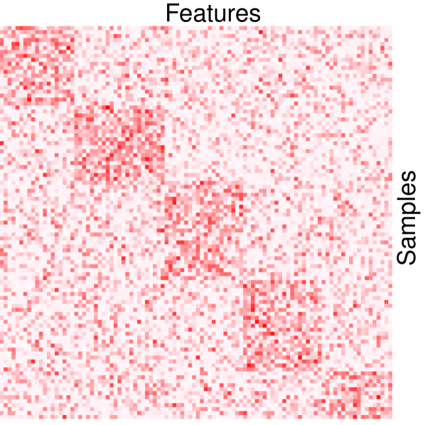
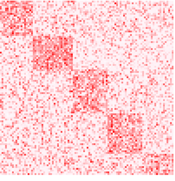
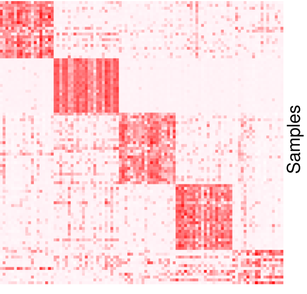
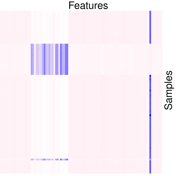
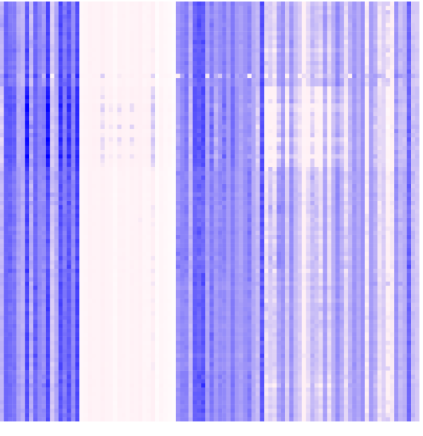
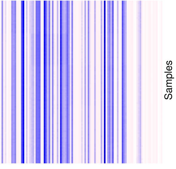
Fig. 1 illustrates a running example of ROCCO vs. a State-of-the-Art (SoA) benchmarking approach, COBRA. Like ROCCO, COBRA learns a data representation to address CoC problem on high-dimensional datasets - particularly focused on Biomedicine applications. However, it formulates the underlying optimization problem as a convex one. While this assumption may hold in some domains, in others it may require a large effort on data preparation to achieve acceptable results. Moreover, in opposition to ROCCO, COBRA is also sensitive to its hyperparameter setting - regarding the number of clusters to be found. The progressive example in Fig. 1 clearly demonstrates that, under a realistic scenario of addressing an input data matrix with a CoC pattern surrounded by the significant amount of noise, ROCCO ’s non-convex approach is more suitable and, therefore, a more generalist solution for this problem. Note that, for this benchmark, the COBRA hyperparameters were tuned using the heuristic originally proposed by the authors in [CAB17].

The contributions of this paper are three-fold:

1. Problem Formulation: A generic problem formulation that includes a clear, continuous and non-convex objective function to perform Co-Clustering;

2. Scalability: A pragmatic solving procedure for learning proved to have theoretical near-linear time complexity on the size of the input matrix. Moreover, we empirically demonstrate that its runtime scales linearly in practice;

3. Robustness: All-in-all, a CoC algorithm that finds co-clusters in a nearly hyperparameter-free fashion, exhibiting low sensitivity to different settings when evaluated empirically.

Over the next sections of this paper, we formally introduce the proposed algorithm, the mathematical proofs that sustain its properties and a comprehensive experimental setup that benchmarks ROCCO against the SoA on this topic resorting to multiple large-scale synthetic datasets, as well as to cross-domain ones.

(a) Initial Toy Dataset.

(b) Toy Dataset with added noise.

(c) SoA [CAB17] representation.

(d) Our representation.

Figure 1: ROCCO’s benchmarking example.

2 Robust Continuous Co-Clustering

2.1 Problem Formulation

Consider a dataset with $n$ samples $X=\{x_{1},x_{2},...,x_{n}\}\in\mathbb{R}^{n\times p}$ with $p$ features each as input. COBRA [CAB17] is a recent approach to CoC. It settles on a convex optimization problem that learns a graph-based representation of the latent co-clusters structure. It operates in three straightforward steps: (1) firstly, it constructs two graphs $G_{p}$ and $G_{f}$ on the samples and features of $X$, e.g. $k$-nearest neighbor on Euclidean space of $X$. Secondly (2), COBRA aims to learn a compact representation $U=\{u_{1},u_{2},...,u_{n}\}=\{u^{1},u^{2},...,u^{p}\}\in\mathbb{R}^{n\times p}$ of $X$ so that $u_{i}$ and $u_{j}$ are similar if samples $i$ and $j$ are connected in $G_{p}$, $u^{i}$ and $u^{j}$ are similar if features $i$ and $j$ are connected in $G_{f}$.

This problem can be formulated as follows:

$$\min_{U}||X-U||_{F}^{2}+\frac{\alpha}{2}\sum\nolimits_{i,j\in E_{p}}||u_{i}-u_{j}||_{2}+\frac{\beta}{2}\sum\nolimits_{i,j\in E_{f}}||u^{i}-u^{j}||_{2}$$ (1)

where $\alpha$ and $\beta$ balance the relevance of the correspondent terms. Finally, the (3) clustering assignment is based on newly learned representation $U$, where the cluster structure is highlighted.

Despite being elegant, the convexity imposed by Eq. (1) may not adequately address the patterns in the input data matrix (e.g. see Fig. 1). Also recently, Shah and Koltun [SK17] proposed a solution for classical clustering problems that overcomes this limitation: the Robust Continuous Clustering (RCC) algorithm. Its problem formulation settles on a non-convex optimization objective function:

$$\min_{U}\frac{1}{2}\sum\nolimits_{i=1}^{n}||x_{i}-u_{i}||_{2}^{2}+\frac{\alpha}{2}\sum\nolimits_{i,j\in E_{p}}\rho(||u_{i}-u_{j}||_{2})$$ (2)

where the non-convexity comes from the regularization function $\rho$. In [SK17], the authors propose the Geman-McClure function as $\rho$:

$$\rho(y)=\frac{\mu y^{2}}{\mu+y^{2}}$$ (3)

where $\mu$ controls the function’s convexity.

Although the optimization problem is non-convex, RCC achieves SoA clustering accuracy. Moreover, it automatically learns the regularization parameter $\alpha$ and non-convexity parameter $\mu$. The idea of using $L_{2}$ norm in regularization is to enforce the learned representatives $u_{i}$ from the same cluster to collapse into a single point. RCC authors [SK17] noted that convex functions have limited robustness to spurious edges in the graph. Consequently, their influence does not diminish during optimization. Therefore, the proposed non-convex function naturally overcomes this issue.

Departing from this idea, we firstly formulate ROCCO’s problem by naturally adapting the optimization objective function of RCC from clustering to the CoC problem. It goes as follows:

$$\min_{U}||X-U||_{F}^{2}+\frac{\alpha}{2}\sum_{i,j\in E_{p}}\rho(||u_{i}-u_{j}||_{2})+\frac{\beta}{2}\sum_{i,j\in E_{f}}\rho(||u^{i}-u^{j}||_{2})$$ (4)

Moreover, we also choose to inherit the straightforward non-convex function defined in (Eq. (3)).

Departing from the ideas introduced by both COBRA and RCC, ROCCO’s problem formulation introduced in Eq. (4) is natural and straightforward. However, the solution of such optimization problem in a scalable fashion is far from trivial (e.g. the optimization solver proposed in COBRA cannot address the non-convex problem enunciated in Eq. (4)). In the next section, we propose a novel method to solve Eq. (4) efficiently.

2.2 Optimization

The solver originally proposed for RCC is based on the duality between robust estimation and line processes. We follow the same idea to optimize Eq. (4). To do it so, we start by introducing two auxiliary variables: $L_{p}(i,j)$ for connections $(i,j)\in E_{p}$; and $L_{f}(i,j)$ for connections $(i,j)\in E_{f}$. Using those, we can re-write Eq. (4) as:

$$\begin{split}\min_{U,L_{p},L_{f}}||X-U||_{F}^{2}+\frac{\alpha}{2}\sum\nolimits_{i,j\in E_{p}}(L_{p}(i,j)||u_{i}-u_{j}||_{2}^{2}+\Psi(L_{p}(i,j)))\\ +\frac{\beta}{2}\sum\nolimits_{i,j\in E_{f}}(L_{f}(i,j)||u^{i}-u^{j}||_{2}^{2}+\Psi(L_{f}(i,j)))\end{split}$$ (5)

As shown in [SK17], Eqs. (4,5) are equivalent with respect to the representation $U$ and function $\rho$ when

$$\Psi(z)=\mu(\sqrt{z}-1)^{2}$$ (6)

The objective in Eq. (5) is biconvex on $(U,L_{p})$ and $(U,L_{f})$. When $U$ is fixed, the optimal value of $L_{p}$ and $L_{f}$ can be derived in closed form. If variables $L_{p}$ and $L_{f}$ are fixed, Eq. (5) turns into solving a Sylvester equation. Therefore, we optimize the objective by alternating optimization. When $U$ is fixed, we can take the partial derivative of Eq. (5) regarding $L_{p}$ and $L_{f}$ and set them to zero. This way, we get the update rules for $L_{p}$ and $L_{q}$ as follows:

$$\begin{split}L_{p}(i,j)=(\frac{\mu}{\mu+||u_{i}-u_{j}||^{2}_{2}})^{2}\\ L_{f}(i,j)=(\frac{\mu}{\mu+||u^{i}-u^{j}||^{2}_{2}})^{2}\end{split}$$ (7)

If we only consider $L_{p}$ in Eq. (5) and discard the $L_{f}$ part, we can rewrite Eq. (5) with $L_{p}$ fixed as:

$$\min_{U}\frac{1}{2}||X-U||_{F}^{2}+\frac{\alpha}{2}\sum\nolimits_{i,j\in E_{p}}L_{p}(i,j)||U(e_{i}-e_{j})||_{2}^{2}$$ (8)

where $e_{i}\in\mathbb{R}^{n}$ is an indicator vector with the $i$th element set to $1$ and others set to $0$. Notoriously, the problem enunciated in Eq. (8) is similar to the RCC one described in Eq. (2).

Taking the derivative of Eq. (8) and setting it to zero, the solution equals to the following linear least-squares problem:

$$\begin{split}&AU=X,\text{where}\\ &A=I+\alpha\sum\nolimits_{i,j\in E_{p}}L_{p}(i,j)(e_{i}-e_{j})(e_{i}-e_{j})^{T}\end{split}$$ (9)

Following a similar rationale, if we only consider $L_{f}$ in Eq. (5), the optimal $U$ can be derived by solving yet another linear least-squares problem:

$$\begin{split}&UB=X,\text{where}\\ &B=I+\alpha\sum\nolimits_{i,j\in E_{f}}L_{f}(i,j)(e^{i}-e^{j})(e^{i}-e^{j})^{T}\end{split}$$ (10)

where $e^{i}\in\mathbb{R}^{p}$ is an indicator vector.

Therefore, when $L_{p}$ and $L_{f}$ are fixed, the optimal $U$ equals to the solution of the following Sylvester equation:

$$AU+UB=2X$$ (11)

where $A$ and $B$ are defined as in Eq. (9) and (10).

In practice, we propose to address Eq. (4) by performing alternating updates of $L_{p}$ and $L_{f}$ (using Eq. (7)) and solving the Sylvester equation in Eq. (7) until convergence. However, classical solutions for the latter problem get expensive when scaled up to massive datasets. A illustrative example of a common solver for the Sylvester Equation is the Bartels-Stewart algorithm [BS72], which has a time complexity of $\mathcal{O}(n^{3}+p^{3})$. This issue turns this procedure not easily applicable in large-scale CoC problems.

To address this challenge, we propose to solve the Sylvester equation using the Kronecker product. Departing from the observation that matrices $A$ and $B$ are sparse, Eq. (11) can be rewritten as

$$\begin{split}C\cdot vec(U)=vec(X),\text{where}\\ C=A\otimes I_{p}+B\otimes I_{n}\end{split}$$ (12)

Eq. (12) is a linear least-squares problem on a sparse matrix $C$. A classical solution for sparse linear systems is the Conjugate Gradient method [HS52]. Note that $A$ and $B$ relate to the $k$-nearest neighbor graphs on the data with $n$ samples and $p$ features. Therefore, there are $\mathcal{O}(n)$, $\mathcal{O}(p)$, and $\mathcal{O}(np)$ non-zero entries in $A$, $B$ and $C$, respectively. The classic Conjugate Gradient method runs with the complexity of $\mathcal{O}(n^{2}p^{2})$, which is even worse compared to the Bartels-Stewart algorithm (assuming large values for $n$ and $p$).

In this paper, we recognize that there is a critical property of matrix $C$ in Eq. (12): $C$ is symmetric diagonally dominant, which enables the usage of a near linear method to solve Eq. (12).

Definition 2.1

Symmetric Diagonally Dominant

Matrix $A$ is symmetric diagonally dominant, if $A$ is symmetric and

$$A(i,i)\geq\sum_{i\neq j}|A(i,j)|$$ (13)

The equality holds when $A$ is a Laplacian matrix.

Theorem 2.1

Matrix $A$ and $B$ defined in Eq. (9) and (10) are Symmetric Diagonally Dominant.

Proof.

Let $N_{ij}\in\mathbb{R}^{n\times n}$ and $N_{i,j}=(e_{i}-e_{j})(e_{i}-e_{j})^{T}$, thus $N_{i,j}$ is a Laplacian matrix. Therefore, $L_{p}(i,j)N_{i,j}$ is a Laplacian matrix as well, since $L_{p}(i,j)\geq 0$. The sum of Laplacian matrices is also a Laplacian matrix, thus $N=\sum_{i,j\in E_{p}}L_{p}(i,j)N_{i,j}$ is also a Laplacian matrix with $N(i,i)=\sum_{i\neq j}|N(i,j)|$. Therefore $A=I+\alpha N$ with $A(i,i)=\sum_{i\neq j}|A(i,j)|+1$ is symmetric diagonally dominant. The same proof applies to $B$ as well. ∎

Theorem 2.2

Matrix $A\otimes I_{p}$ is symmetric diagonally dominant if $A\in\mathbb{R}^{n\times n}$ is symmetric diagonally dominant.

Proof.

$A\otimes I$ is symmetric, since both $A$ and $I_{p}$ are symmetric. Consequently, we have

$$M=A\otimes I=I\otimes A=\begin{bmatrix}A&\dots&0\\ \vdots&\ddots&\vdots\\ 0&\dots&A\end{bmatrix}$$ (14)

where $A(i,i)\geq\sum_{i\neq j}|A(i,j)|$, thus $M(i,i)\geq\sum_{i\neq j}|M(i,j)|$. This turns $A\otimes I_{p}$ to be a symmetric diagonally dominant matrix. ∎

As $C$ is symmetric diagonally dominant, many theoretic studies have shown that Eq. (12) can be solved in near linear time (i.e. $\mathcal{O}(m\log(m))$) with respect to the $m$ non-zero entries in $C$ [KMP11, CKM⁺14, KOSZ13]. Besides these theoretic solvers, there are already toolboxes that can solve Eq. (12) with empirically linear observation (e.g. Combinatorial MultiGrid (CMG) algorithm [IMT11]).

In this paper, we propose to use CMG to solve Eq. (12).

2.3 Algorithm’s Overview

ROCCO is summarized in Algorithm 1. As input, ROCCO takes a data matrix $X\in\mathbb{R}^{n\times p}$. Its output are clustering assignments of both samples $C_{p}$ and features $C_{f}$. Firstly, it constructs the graphs on samples $G_{p}$ and features $G_{f}$ separately. Following [SK17], we also propose to use mutual $k$-nearest neighbor connectivity [BCQY97], which is more robust than the commonly used $k$-NN graphs.

Initialization.

We initialize the representation $U$ to $X$. The auxiliary variables $L_{p}(i,j)$ and $L_{f}(i,j)$ are assigned to $1$ whenever the edge $(i,j)$ exists in the graphs $G_{p}$ and $G_{f}$, respectively. Finally, the regularization parameters $\alpha$ and $\beta$ are initialized as follows:

$$\alpha=\frac{||X||_{2}}{||P||_{2}},\beta=\frac{||X||_{2}}{||Q||_{2}}$$ (15)

where $P=\sum\nolimits_{i,j\in E_{p}}L_{p}(i,j)(e_{i}-e_{j})(e_{i}-e_{j})^{T}$ and $Q=\sum\nolimits_{i,j\in E_{f}}L_{f}(i,j)$ $(e^{i}-e^{j})(e^{i}-e^{j})^{T}$. Eq. (15) balances both the data and pairwise terms in Eq. (4).

Iteration.

Then, ROCCO iterates on optimizing the proposed objective function by updating $L_{p}$, $L_{f}$ and $U$ alternatively until convergence (as described in Section 2.2). The parameter $\mu$ that controls the (non-)convexity of $\rho$ is proposed to be updated using graduated non-convexity. It begins with a locally convex approximation of the objective, obtained by setting a large enough $\mu$. Then, $\mu$ is automatically decreased every four iterations in order to introduce non-convexity into the objective on a gradual fashion. Under certain assumptions, such continuation schemes are known to attain solutions that are close to the global optimum [MFI15]. Eq. (15) is applied to update $\alpha$ and $\beta$ after every update of $\mu$, so that $\alpha$ and $\beta$ are automatically determined.

Input : Data matrix $X\in\mathbb{R}^{n\times p}$.

Output : Co-Cluster assignments $C_{p}$, $C_{f}$.

1 Construct mutual $K$-nearest neighbor graphs $E_{p}$ and $E_{f}$;

2 Initialize $U=X$, $L_{p}(i,j)=1$, $L_{f}(i,j)=1$, $\alpha=\frac{||X||_{2}}{||P||_{2}}$, $\beta=\frac{||X||_{2}}{||Q||_{2}}$, $\mu_{p}\gg\max||x_{i}-x_{j}||^{2}_{2}$, $\mu_{f}\gg\max||x^{i}-x^{j}||^{2}_{2}$;

3 while not converge do

4       Update $L_{p}$ and $L_{f}$ using Eq. (7);

5       Update $A$ and $B$ using Eq. (9) and (10);

6       Update $U$ by solving Eq. (12) using CMG [IMT11];

7       Every four iterations, update $\alpha=\frac{||X||_{2}}{||P||_{2}}$, $\beta=\frac{||X||_{2}}{||Q||_{2}}$, $\mu_{p}=\frac{\mu_{p}}{2}$, $\mu_{f}=\frac{\mu_{f}}{2}$

8 end while

9

10if X is sparse then

       $C_{p}$ = KM($U$);

        // $K$ chosen by Silhouette Coef. [Rou87]

       $C_{f}$ = KM($U^{T}$);

        // $K$ chosen by Silhouette Coef. [Rou87]

11      

12 else

13       $C_{p}$ = RCC($U$) ;

14       $C_{f}$ = RCC($U^{T}$) ;

15      

16 end if

17

18return Co-cluster assignments $C_{p}$ and $C_{f}$;

Algorithm 1 ROCCO

Co-Cluster Assignment.

RCC authors [SK17] suggest to derive the clustering assignment automatically from the connected component of a new graph calculated on $U$ with a heuristic-based threshold. However, we empirically observed that this heuristic does not work for ROCCO. The main issue is that the threshold is calculated on the original input space, pushing the output to provide multiple single point clusters. To tackle this challenge, we propose to employ RCC explicitly on both rows and columns of the new representation $U$ to achieve the final clustering assignment. Intuitively, when facing a sparse input matrix $X$, we may again expect issues with the threshold originally proposed in [SK17]. To mitigate this issue, we suggest to firstly employ a sparsity test on $X$. If positive, we then propose to simply adopt KM instead for final clustering assignment. The number of clusters $K$ is thereby determined by the Silhouette Coefficient [Rou87].

Complexity Analysis.

The runtime complexity of ROCCO is three-fold: (1) graph construction, (2) representation learning, and (3) clustering assignment. For any input dataset $X\in\mathbb{R}^{n\times p}$, (1) the mutual $k$-nearest neighbor graph on either samples or features runs naively $\mathcal{O}(n^{2}p)$ and $\mathcal{O}(np^{2})$, respectively. However, this step can be easily parallelized and there are many studies for approximated $k$-NN graphs construction which can significantly accelerate the runtime in practice [DML11, CFS09]. The computational complexity of representation learning (2) is reduced to solving the Sylvester equation in Eq. (4). Theoretically, it can be solved in $\mathcal{O}(np\mbox{ }log(np))$. However, empirically we observe $\mathcal{O}(np)$. Finally, the co-clustering assignment procedure (3) runs either in $\mathcal{O}(np)$ or $\mathcal{O}(n^{2}p+np^{2})$ using RCC and KM, respectively. Note that KM scales linearly, but the Silhouette-based model selection procedure scales quadratically.

3 Experiments

We aim to evaluate the benefits of ROCCO when compared to other SoA methods for CoC by answering the following questions:

1. Is the representation learned by ROCCO suitable for CoC?

2. Is ROCCO’s clustering assignment fairly good in practice?

3. Can ROCCO handle noisy and/or sparse inputs?

4. Is ROCCO robust to its hyperparameter setting?

5. Does ROCCO empirically scale linearly in the input size?

To handle these questions, we prepared an extensive empirical experimental setup. Its settings are presented below, followed by the testbed details and their results. Finally, we present a comprehensive discussion on the answers that they provide.

3.1 Experimental Setup

We briefly present the comparison partners and their settings, the datasets used to evaluate those, as well as the employed metrics.

3.1.1 SoA Benchmarkers

To benchmark ROCCO, we employed 7 different methods from SoA in (automated) clustering (3) and CoC (4). They are enumerated as follows:

1. KM: $K$-means clustering: probably, the most widely used clustering algorithm;

2. HDBS: Hierarchical Density-Based Clustering [CMS13] eliminates DBSCAN [EKS⁺96] need to cut-off the resulting dendrogram. Instead, the final clusters are automatically determined by traversing a tree of condensed view splits, allowing clusters of different densities.

3. RCC: Robust Continuous Clustering [SK17] learns a regularized graph representation for classical clustering.

4. SCC: Spectral Co-Clustering [Dhi01] treats the input data matrix as a bipartite graph and performs a normalized cut on the graph for clustering assignment.

5. SBC: Spectral Bi-Clustering [KBCG03] performs Single Value Decomposition (SVD) to approximate the original matrix, followed by KM to find the sample and feature clusters.

6. COBRA: Convex Bi-Clustering [CAB17] learns a new representation regularized by both sample and feature graphs with a convex function.

7. COBRAr: To make a fair comparison, we also perform RCC or KM on the learned representation of COBRA for cluster assignment - following strictly the ROCCO’s specific procedure for this task.
   

Implementations.

We used Python implementations of KM, SCC and SBC from the package SciKit-Learn [PVG⁺11]; a fast Python implementation of HDBSCAN from McInnes and Healy [MH17]; a Matlab implementation of RCC [SK17] and an R implementation of COBRA [CAB17].

ROCCO is implemented in Matlab .

Hyperparameter Setting.

KM, SCC, and SBC require the number of clusters to be predetermined. HDBS requires to set min_cluster_size (i.e. the minimum cluster mass), hereby set to $10$. RCC, COBRA and ROCCO learn graphs from the data input. Hereby, all use the mutual $K$-nearest neighbor graph, where $K=10$. Nearest neighbors are calculated by Euclidean distance, except for Text Mining datasets - where cosine distance is used. COBRA is used with the default settings of "cobra_validate" function, where the regularization hyperparameter ($RH$) is automatically set by cross-validation - as suggested by the authors in [CAB17] - over the following grid: $[10^{-3},10^{3}]$.

3.1.2 Datasets

We employ three different types of datasets: (i) Synthetic and Real-World ones. The latter concern two relevant application domains where CoC problem is common: (ii) Text Mining (documents) and (iii) Biomedicine (gene expression). Details about these types are provided below.

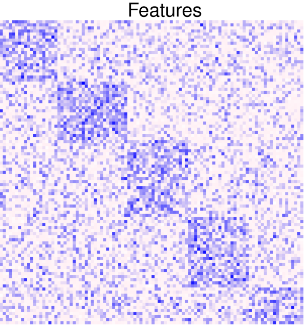
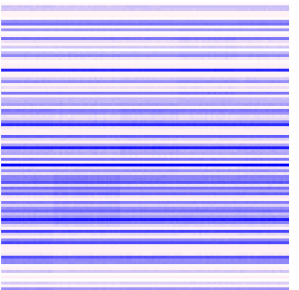
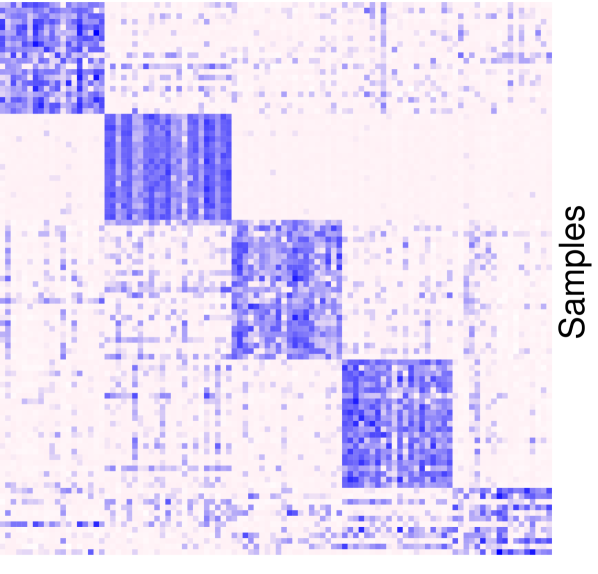
1. Synthetic: We generated synthetic datasets using the function make_biclusters of Python package SciKit-Learn [PVG⁺11]. It creates a matrix of small values and implants co-clusters with large values (e.g. Fig. 1-a). We set both the number of samples and features to $100$, and the number of clusters to $5$. Moreover, we gradually increase the noise level (parameter of make_biclusters) from $10$ to $50$ (e.g. Fig. 1-b). For each possible configuration pair, we generate $30$ datasets with random seed from $0$ to $29$.

2. Text Mining: We employ $5$ document datasets. Classic3 is composed of abstract of papers from three domains and was used in [Dhi01]. We follow [DMM03] to generate 2 subsets of 20-Newsgroup [Lan95]: 20news2 and 20news10. Reuters and RCV1 used in [SK17] are also employed. Each document is represented as the term-frequency inverse document-frequency scores of the top $2000$ most frequent words in their corpus.

3. Biomedicine: We evaluate on $4$ gene expression datasets preprocessed by Nie et al. [NHCD10]: ALLAML, Carcinom, GLIOMA and Lung. Feature scaling is performed beforehand.

Table 1 shows statistics about the real-world datasets (ii,iii).

3.1.3 Evaluation metrics

In the synthetic datasets, we know both the true cluster labels for both samples and features. In the real-world, we only know the sample labels. Therefore, we use Normalized Mutual Information (NMI) [VEB10] for evaluation, which measures the dependence between true labels and the obtained labels. However, other studies [SK17] point that NMI value is biased on the number of clusters. Consequently, different numbers of clusters are often obtained by the evaluated methods. To address this issue, we further evaluate the clustering performance using Adjusted Mutual Information (AMI) [VEB10] and Adjusted Rand Index (ARI) [HA85], whenever the true labels are available.

3.2 Testbeds and Results

In this Section, we describe the testbeds built to answer the proposed research questions, pointing out the obtained results.

Representation Learning (Q1).

In this scenario, we evaluate the goodness of the representation learned by ROCCO for CoC.

Regarding the synthetic datasets, we compare the learned representations by visualizing the resulting heatmaps in Figs. 1 and 2. Figs. 1-(a,b) illustrate well this problem setting: the original synthetic datasets without and with noise of level $50$, respectively. Fig. 1-(c) already illustrated the behavior of COBRA by tuning its $RH$ as originally suggested in [CAB17] (i.e. $RH=10$). However, we extended this evaluation by plotting COBRA’s representation for different levels of $RH$, together with either the samples/features clustering made by RCC. The resulting heatmaps are depicted in Fig. 2.

Table 1: Summary statistics of the real-world datasets.

Domain	Name	Samples	Features	Clusters
	Classic3	3891	2000	3
	20news2	1777	2000	2
Text Mining	20news10	9607	2000	10
	Reuters	9082	2000	50
	RCV1	10000	2000	4
	ALLAML	72	7129	2
	Carcinom	174	9182	11
Biomedicine	GLIOMA	50	4434	4
	Lung	203	3312	5

The real-world datasets are used as follows: KM is performed over the representations $U$ learned by ROCCO, RCC and COBRA. In this case, KM receives the true number of classes as input for either samples and features. KM is also evaluated when using directly over the input matrix, along with SCC and SBC. Similarly, these algorithms are also fed with the real number of classes. If the true number of feature clusters is not known, we assume it to be equal to the samples one. HDBS was deliberately discarded in this evaluation since it is not possible to set the number of clusters apriori for this method. NMI and AMI values for the obtained results are displayed in Table 2.

Real-World Problems (Q2,Q3).

Hereby, we evaluate the performance of ROCCO in practice, where the number of clusters is unknown apriori. HDBS, RCC, COBRA, COBRAr and ROCCO automatically output both row and column clusters. However, KM, SCC, and SBC require the number of clusters to be defined beforehand. To tackle such issue, we adopt a grid search procedure over the number of clusters on $[2,20]$, using then the Silhouette Coefficient [Rou87] for model selection purposes. The resulting methods are then denoted as autoKM, autoSCC, and autoSBC, respectively. To allow a fair comparison in this particular setup, we employ the sparsity test (i.e. document datasets are typically highly sparse) already proposed in the cluster assignment stage of ROCCO also for RCC and COBRAr.

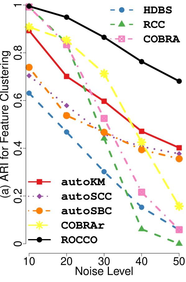
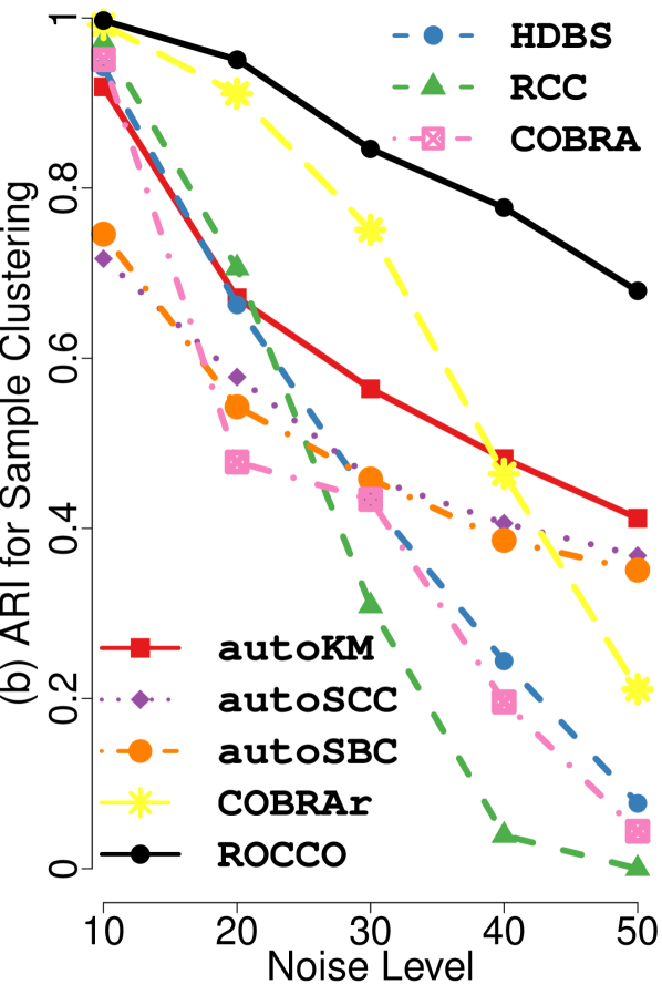
Again, we devised two evaluation test beds: a (i) synthetic and a (ii) real-world one. The first (i) consists on synthetic datasets with gradually increased noise levels (from $10$ to $50$). The (ii) real-world datasets were used as is. Results using the ARI for the clustering procedures over either the samples or the features of the synthetic datasets (i) are depicted in Fig. 3. NMI and AMI values for the results obtained over the (ii) real-world datasets are displayed in Table 3.

(a) COBRA with $RH=1$.

(b) COBRA with $RH=100$.

(c) COBRA with $RH=1000$.

(d) RCC over the samples.

(e) RCC over the features.

(f) ROCCO.

Figure 2: Comparison between the Representations obtained from COBRA, RCC and ROCCO.

Table 2: Representation Learning Results. COBRA, RCC and ROCCO representations were used as input for KM. True number of clusters was given to all the compared methods. Last row depicts the methods average rank per metric.

	KM		RCC +KM		SCC		SBC		COBRA +KM		ROCCO +KM
	NMI	AMI	NMI	AMI	NMI	AMI	NMI	AMI	NMI	AMI	NMI	AMI
Classic3	0.706	0.703	0.909	0.908	0.908	0.905	0.911	0.908	0.716	0.714	0.915	0.914
20news2	0.657	0.650	0.659	0.654	0.005	0.001	0.010	0.001	0.620	0.618	0.806	0.802
20news10	0.219	0.201	0.314	0.266	0.475	0.396	0.264	0.192	0.123	0.102	0.438	0.394
Reuters	0.421	0.307	0.475	0.362	0.408	0.316	0.137	0.077	0.446	0.332	0.540	0.397
RCV1	0.404	0.398	0.394	0.389	0.343	0.310	0.049	0.044	0.398	0.395	0.403	0.393
ALLAML	0.129	0.117	0.007	0.008	0.189	0.177	0.125	0.112	0.171	0.158	0.154	0.141
Carcinom	0.648	0.588	0.778	0.719	0.373	0.246	0.443	0.341	0.651	0.593	0.794	0.745
GLIOMA	0.537	0.478	0.484	0.411	0.085	0.001	0.151	0.073	0.507	0.450	0.484	0.411
Lung	0.658	0.557	0.649	0.557	0.391	0.368	0.451	0.366	0.661	0.562	0.711	0.645
$\varnothing$ Rank	3.444	3.500	3.277	3.166	4.444	4.166	4.777	5.111	3.333	3.222	1.722	1.833

Table 3: Real-world Benchmark where the real $K$ is not given. autoKM, autoSCC, and autoSBC follow a grid-search procedure over a pool of $K$ values to then select the best model using the Silhouette Coef.. The remaining methods choose $K$ automatically.

	autoKM		HDBS		RCC		autoSCC		autoSBC		COBRA		COBRAr		ROCCO
	NMI	AMI	NMI	AMI	NMI	AMI	NMI	AMI	NMI	AMI	NMI	AMI	NMI	AMI	NMI	AMI
Classic3	0.704	0.701	0.019	0.014	0.903	0.903	0.906	0.903	0.914	0.912	0.362	0.001	0.715	0.713	0.914	0.913
20news2	0.293	0.169	0.052	0.050	0.391	0.333	0.005	0.001	0.010	0.001	0.303	0.001	0.358	0.212	0.806	0.802
20news10	0.290	0.275	0.155	0.071	0.349	0.333	0.274	0.098	0.037	0.003	0.500	0.001	0.290	0.279	0.495	0.479
Reuters	0.271	0.160	0.172	0.071	0.252	0.146	0.280	0.168	0.034	0.018	0.479	0.001	0.270	0.159	0.295	0.163
RCV1	0.466	0.311	0.165	0.140	0.454	0.325	0.346	0.313	0.012	0.001	0.367	0.001	0.483	0.346	0.462	0.363
ALLAML	0.154	0.141	0.001	0.001	0.007	0.001	0.189	0.177	0.125	0.112	0.208	0.023	0.001	0.001	0.279	0.158
Carcinom	0.659	0.599	0.499	0.332	0.474	0.215	0.388	0.155	0.270	0.099	0.680	0.062	0.430	0.173	0.791	0.743
GLIOMA	0.630	0.432	0.398	0.300	0.476	0.379	0.050	0.011	0.154	0.089	0.587	0.001	0.174	0.064	0.484	0.411
Lung	0.550	0.314	0.401	0.290	0.557	0.303	0.306	0.128	0.505	0.287	0.496	0.319	0.737	0.605	0.602	0.389
$\varnothing$ Rank	3.722	3.555	6.500	5.555	4.111	3.833	5.777	4.722	6.388	5.944	3.333	6.944	4.333	4.000	1.833	1.444

Figure 3: Noise-based benchmark on Synthetic datasets over either samples and features using ARI. Best viewed in color.

Robustness (Q4).

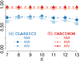
ROCCO possesses two hyperparameters used to construct the initial graph: (i) $K$ for the mutual $K$-nearest neighbor graph; and (ii) the used distance function. We empirically evaluate its robustness over two grid of values defined as $K=\{7..13\}$ and distance_Function = {(E)uclidean, (M)anhattan, (C)osine}, respectively. Fig. 4 illustrates the results obtained on two real-world datasets: Classic3 and Carcinom.

	NMI	AMI	ARI
E (a)	0.9157	0.9148	0.9541
M (a)	0.9144	0.9136	0.9525
C (a)	0.9157	0.9148	0.9507
VAR	5.6$\mathrm{e}^{-7}$	4.8$\mathrm{e}^{-7}$	1.6$\mathrm{e}^{-7}$
E (b)	0.7911	0.7432	0.7063
M (b)	0.7911	0.7432	0.7063
C (b)	0.7911	0.7432	0.7063
VAR	0.0000	0.0000	0.0000

Figure 4: Sensitivity Analysis to ROCCO’s hyperparameters used to build the initial graph, considering both (a) CLASSIC3 and (b) (CARCINOM) datasets. The chart on left depicts an analysis of $K$, the number of neighbors. The Table on right depicts the results for the (E)uclidean, (M)anhattan and (C)osine distance metrics, as well as their respective VARiance.

Scalability (Q5).

Figure 5: Empirical Scalability Evaluation using synthetic data with different sample sizes (x-axis). Top chart depicts the analysis of runtime complexity of the 3 stages of ROCCO: (1) graph generation, (2) representation learning and (3) clustering assignment. Bottom one benchmarks ROCCO vs. its comparison partners. Best viewed in color.

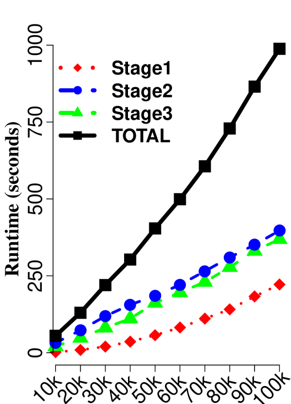
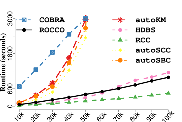
To evaluate scalability empirically, we generated 10 datasets with fixed feature size (i.e. $p=100$), $\{10..100\}\times 10^{3}$ samples and a residual noise level (i.e. 10). These datasets are used to benchmark ROCCO against its comparison partners. Fig. 5 illustrates the obtained results, adding also detailed analysis about the running times of the different ROCCO stages. Note that the auto* methods include the Silhouette-based model selection procedure.

3.3 Discussion

In this section, we discuss the results to see whether they answer the five research questions we proposed to address with these experiments.

Representation Learning (Q1).

From the heatmaps in Figs. 1 and 2, it can be clearly seen that the representation learned by ROCCO (Fig. 2-(f)) on the synthetic dataset successfully discovers the underlining Co-clustering structure (Fig. 1-(a)). On the other hand, the representations learned by COBRA do not highlight that structure so well - even when varying $RH$ exhaustively (Fig. 2-(a,b,c)). In the same line, RCC also fails to discover such structure when addressing directly either samples or features individually (Fig. 2-(d,e)).

Table 2 highlights that ROCCO has top-performance on $6$ and $5$ out of the $9$ datasets, the second best on $2$ and $3$ other datasets, accordingly to NMI and AMI, respectively. We have a similar observation on the results of ARI as well. In sum, ROCCO ranks in the first place on both metrics, followed by RCC and COBRA.

These results show the essential of the objective formulation of ROCCO and its advancement compared to SoA methods regarding representation learning for CoC.

Real-World Problems (Q2, Q3).

Not surprisingly, after observing Fig. 3, we can conclude that all methods performance is inversely proportional to the noise level (NMI and AMI results are similar). Yet, ROCCO is by far the least affected method: it provides an ARI of $0.68$ on either samples and features for the highest noise level, where the second best method (i.e. autoKM) only achieves an ARI of $0.41$. Moreover, COBRAr also outperforms COBRA in most cases. This fact shows the effectiveness of ROCCO’s clustering assignment strategy.

Table 3 uncovers that ROCCO also achieves high performance when facing real-world datasets from multiple domains. ROCCO outperforms its counterparts on $4$ and $5$ out of the $9$ datasets, on NMI and AMI, respectively. Moreover, it is possible to conclude that it achieves almost always the second best on all the remaining datasets. Naturally, ROCCO ranks in the first place on both metrics, followed by COBRA and autoKM for NMI and AMI separately. Please note that COBRA provides good NMI results, but poor AMI results, since it typically produces a large number of clusters.

These results are illustrative of the effectiveness of ROCCO on real-world CoC problems. However, the clustering assignment of ROCCO is fully data dependent - which may raise some issues. Consider the following example: if we use RCC to generate the final clustering of the representations learned on sparse datasets (e.g. text documents), we will obtain single points clusters. To tackle this challenge, we proposed (in Section 2.3) to apply autoKM instead after representation learning. Notoriously, this approach achieves promising results (Table 3). However, this comes at the cost of increasing both ROCCO’s runtime (Silhouette-based model selection) and its sensitivity to outliers (inherited from KM).

Robustness (Q4).

Fig. 4 shows that ROCCO performs stable with near zero variance across different distance functions on both evaluated datasets. Regarding $K$, ROCCO performs stable on CARCINOM dataset with all $K$’s and on CLASSIC3 with $K=8,9,10$. However, it degrades its performance slightly with other $K$ values. The sensitivity may also be inherited from the usage of KM in the clustering assignment stage (for sparse datasets). Overall, we can say that ROCCO’s performance is robust against its hyperparameters.

Scalability (Q5).

Top chart in Fig. 5 depicts the runtime of 3 stages of ROCCO, where the runtime of stage $1$ (graph generation) scales quadratically, while stages $2$ (representation learning) and $3$ (clustering assignment) scale nearly linearly. Overall, ROCCO’s total runtime complexity is slightly over a linear one, since the quadratical part is still the cheapest even for $100k$ samples.

Bottom chart in Fig. 5 depicts that ROCCO, RCC, COBRA, and HDBS scale nearly linear, while the runtime of auto* methods scales clearly in a quadratic scale. As mentioned before, the quadratic complexity of all auto* methods is due to Silhouette-based model selection. KM, SCC, and SBC scale linearly when the number of clusters is given beforehand. Although possessing a linear runtime curve, COBRA turns to be quite expensive when compared to remaining partners. This slope derives from its heuristic to tune $RH$, which involves to re-run the algorithm multiple times.

By the above-mentioned reasons, all the five research questions can be answered affirmatively.

4 Related Work

In this Section, we briefly review the SoA with respect to CoC, as well as to two related topics: Parameter-free and Continuous Clustering.

4.1 Co-Clustering

CoC has been extensively studied in the literature, which works on high-dimensional data and increases the interpretability compared to classical clustering. SCC [Dhi01] is one of the earliest works on co-clustering documents and words. It treats the input data matrix as a bipartite graph and performs the normalized cut on the graph. SBC from Kluger et al. [KBCG03] is another SoA method for CoC gene expression data. SBC performs SVD to approximate the original matrix followed by KM to find the row and column clusters. Later, many CoC methods were proposed. Dhillon et al. proposed an information theory based co-clustering method [DMM03]. Ding et al. proposed a CoC method based on Nonnegative matrix tri-factorization [DLPP06]. Shan and Banerjee proposed Bayesian co-clustering [SB08]. Du and Shen proposed a CoC method with graph regularized Nonnegative matrix tri-factorization [DS13]. Nie et al. proposed to learn a structured optimal bipartite graph for CoC [NWDH17]. However, all these methods require to set hyperparameters beforehand, e.g. the number of clusters, subspace dimensionality or regularizers. Commonly, these hyperparameters settings strongly affect the clustering results. Typically, there are no universal guidelines on how to select them in practice. In contrast to the abovementioned methods, ROCCO learns critical hyperparameters automatically, e.g. regularizers. Moreover, it is robust to other hyperparameters, e.g. $K$ for constructing $K$-nearest neighbor graphs.

4.2 Parameter-free Clustering

Clustering is an unsupervised learning task. Therefore, hyperparameter settings are crucial in practice. Many metrics are proposed to determine the number of clusters for KM. The Silhouette Coefficient has been proposed long ago [Rou87]. Yet, it is still one of the most widely used metrics. Wiwie et al. [WBR15] studies the performance of different clustering metrics and show that the Silhouette Coefficient is the most suitable for bio-medical data. HDBS [CMS13] is a nearly-automatic density-based approach for clustering that eliminates DBSCAN [EKS⁺96] need to cut-off the resulting dendrogram. Instead, the final clusters are determined by traversing a tree of condensed view splits, allowing clusters of different densities to be formed.

The literature on parameter-free methods CoC is scarce. To the best of our knowledge, HiCC [IPM09] is the only method that tries to address this issue in CoC. However, HiCC tries to learn the hierarchy of samples and features together in a parameter-free way - which is a problem distinct from the one in our scope.

4.3 Continuous Clustering

Continuous clustering algorithms attracted attention recently. The main idea is to convert the clustering problem to a continuous optimization problem, where a regularized graph-based representation is learned with good clustering structure. Firstly, [LOL11, HJBV11] proposed to relax the KM clustering and hierarchical clustering to convex optimization problems. The newly learned representation owns a good cluster structure, so that clustering assignment can be achieved from the connected component of the calculated graph. Later, Chi and Lange [CL15] proposed a splitting method to accelerate the solving of the convex optimization problem. All the above-mentioned methods use the convex ($L_{2}$ norm) function for regularization. Recently, Shah and Koltun [SK17] proposed RCC, which uses a non-convex (Geman-McClure) function for regularization. RCC achieves SoA clustering accuracy without setting regularization parameters. The proposed ROCCO can be seen as an extension of RCC to the CoC problem. ROCCO inherited the merits of RCC with high-quality clustering and no regularization parameter setting. Recently, Chi et al. proposed a convex bi-clustering algorithm COBRA [CAB17], which is the most relevant method to the proposed ROCCO. COBRA also learns the representation regularized on both sample and feature graphs. However, COBRA adopts a convex ($L_{2}$ norm) regularization function, while the proposed ROCCO uses a non-convex function for the same purpose. Therefore, the two optimization problems are radically different. ROCCO proposed a new optimization method to solve the resulting non-convex (harder) problem. Finally, ROCCO convincingly outperforms COBRA in our experiments.

5 Final Remarks

In this paper, we formulate CoC as a continuous non-convex optimization problem that settles on a graph-based representation of both samples and features. Further, we present an approach (i.e. ROCCO) that solves this problem with theoretical near-linear time complexity on the input data matrix. Extensive experiments show the effectiveness of the learned representations and the resulting clustering quality. Along with these characteristics, ROCCO’s robustness to hyperparameters, and its scalability on both synthetic and real-world datasets either matches and/or (mostly) outperforms SoA counterparts. ROCCO will serve as a parameter-free CoC method for large-scale problems, regardless of the characteristics of the input data or the application domain.

References

- [BCQY97] M. Brito, E. Chavez, A. Quiroz, and J. Yukich. Connectivity of the mutual k-nearest-neighbor graph in clustering and outlier detection. Statistics & Probability Letters, 35(1):33–42, 1997.
- [BPP08] S. Busygin, O. Prokopyev, and P. Pardalos. Biclustering in data mining. Computers & Operations Research, 35(9):2964–2987, 2008.
- [BS72] R. Bartels and G. Stewart. Solution of the matrix equation ax+xb=c [f4]. Communications of the ACM, 15(9):820–826, 1972.
- [CAB17] E. Chi, G. Allen, and R. Baraniuk. Convex biclustering. Biometrics, 73(1):10–19, 2017.
- [CFS09] J. Chen, H. Fang, and Y. Saad. Fast approximate knn graph construction for high dimensional data via recursive lanczos bisection. Journal of Machine Learning Research, 10(Sep):1989–2012, 2009.
- [CKM+14] M. Cohen, R. Kyng, G. Miller, J. Pachocki, R. Peng, A. Rao, and S. Xu. Solving sdd linear systems in nearly m log 1/2 n time. In Proceedings of the 46th Annual ACM symposium on Theory of computing, pages 343–352. ACM, 2014.
- [CL15] E. Chi and K. Lange. Splitting methods for convex clustering. Journal of Computational and Graphical Statistics, 24(4):994–1013, 2015.
- [CMS13] R. Campello, D. Moulavi, and J. Sander. Density-based clustering based on hierarchical density estimates. In Pacific-Asia conference on Knowledge Discovery and Data mining (PAKDD), pages 160–172. Springer, 2013.
- [Dhi01] I. Dhillon. Co-clustering documents and words using bipartite spectral graph partitioning. In Proceedings of the 7th ACM SIGKDD International Conference on Knowledge Discovery and Data mining (KDD), pages 269–274. ACM, 2001.
- [DLPP06] C. Ding, T. Li, W. Peng, and H. Park. Orthogonal nonnegative matrix t-factorizations for clustering. In Proceedings of the 12th ACM SIGKDD International Conference on Knowledge Discovery and Data mining (KDD), pages 126–135. ACM, 2006.
- [DML11] W. Dong, C. Moses, and K. Li. Efficient k-nearest neighbor graph construction for generic similarity measures. In Proceedings of the 20th International Conference on World Wide Web (WWW), pages 577–586. ACM, 2011.
- [DMM03] I. Dhillon, S. Mallela, and D. Modha. Information-theoretic co-clustering. In Proceedings of the 9th ACM SIGKDD International Conference on Knowledge Discovery and Data mining (KDD), pages 89–98. ACM, 2003.
- [DS13] L. Du and Y. Shen. Towards robust co-clustering. In Proceedings of International Joint Conference on Artificial Intelligence (IJCAI), pages 1317–1322, 2013.
- [EKS+96] M. Ester, H. Kriegel, J. Sander, X. Xu, et al. A density-based algorithm for discovering clusters in large spatial databases with noise. In Proceedings of the 2nd ACM SIGKDD International Conference on Knowledge Discovery and Data mining (KDD), volume 96, pages 226–231, 1996.
- [HA85] L. Hubert and Phipps Arabie. Comparing partitions. Journal of classification, 2(1):193–218, 1985.
- [HJBV11] T. Hocking, A. Joulin, F. Bach, and J. Vert. Clusterpath an algorithm for clustering using convex fusion penalties. In 28th International Conference on Machine Learning (ICML), 2011.
- [HP99] T. Hofmann and J. Puzicha. Latent class models for collaborative filtering. In Proceedings of International Joint Conference on Artificial Intelligence (IJCAI), volume 99, 1999.
- [HS52] M. Hestenes and E. Stiefel. Methods of conjugate gradients for solving linear systems, volume 49. NBS, 1952.
- [IMT11] K. Ioannis, G. Miller, and D. Tolliver. Combinatorial preconditioners and multilevel solvers for problems in computer vision and image processing. Computer Vision and Image Understanding, 115(12):1638 – 1646, 2011.
- [IPM09] Dino Ienco, Ruggero G Pensa, and Rosa Meo. Parameter-free hierarchical co-clustering by n-ary splits. In Joint European Conference on Machine Learning and Knowledge Discovery in Databases, pages 580–595. Springer, 2009.
- [KBCG03] Y. Kluger, R. Basri, J. Chang, and M. Gerstein. Spectral biclustering of microarray data: co-clustering genes and conditions. Genome research, 13(4):703–716, 2003.
- [KMMCC16] J. Khiari, L. Moreira-Matias, V. Cerqueira, and O. Cats. Automated setting of bus schedule coverage using unsupervised machine learning. In Pacific-Asia Conference on Knowledge Discovery and Data Mining (PAKDD), pages 552–564. Springer, 2016.
- [KMP11] I. Koutis, G. Miller, and R. Peng. A nearly-m log n time solver for sdd linear systems. In Foundations of Computer Science (FOCS), 2011 IEEE 52nd Annual Symposium on, pages 590–598. IEEE, 2011.
- [KOSZ13] J. Kelner, L. Orecchia, A. Sidford, and Z. Zhu. A simple, combinatorial algorithm for solving sdd systems in nearly-linear time. In Proceedings of the 45th annual ACM symposium on Theory of computing, pages 911–920. ACM, 2013.
- [Lan95] K. Lang. Newsweeder: Learning to filter netnews. In Machine Learning Proceedings 1995, pages 331–339. Elsevier, 1995.
- [LOL11] F. Lindsten, H. Ohlsson, and L. Ljung. Just relax and come clustering!: A convexification of k-means clustering. Linköping University Electronic Press, 2011.
- [LW03] J. Liu and W. Wang. Op-cluster: Clustering by tendency in high dimensional space. In Data Mining, 2003. ICDM 2003. Third IEEE International Conference on, pages 187–194. IEEE, 2003.
- [MFI15] H. Mobahi and J. Fisher III. A theoretical analysis of optimization by gaussian continuation. In AAAI, pages 1205–1211, 2015.
- [MH17] L. McInnes and J. Healy. Accelerated hierarchical density based clustering. In Data Mining Workshops (ICDMW), 2017 IEEE International Conference on, pages 33–42. IEEE, 2017.
- [MP16] S. Maurus and C. Plant. Skinny-dip: Clustering in a sea of noise. In Proceedings of the 22nd ACM SIGKDD International Conference on Knowledge Discovery and Data mining (KDD), pages 1055–1064. ACM, 2016.
- [NHCD10] F. Nie, H. Huang, X. Cai, and C. Ding. Efficient and robust feature selection via joint l2, 1-norms minimization. In Advances in Neural Information Processing Systems (NIPS), pages 1813–1821, 2010.
- [NWDH17] F. Nie, X. Wang, C. Deng, and H. Huang. Learning a structured optimal bipartite graph for co-clustering. In Advances in Neural Information Processing Systems (NIPS), pages 4132–4141, 2017.
- [PVG+11] F. Pedregosa, G. Varoquaux, A. Gramfort, et al. Scikit-learn: Machine learning in Python. Journal of Machine Learning Research, 12:2825–2830, 2011.
- [Rou87] P. Rousseeuw. Silhouettes: a graphical aid to the interpretation and validation of cluster analysis. Journal of computational and Applied Mathematics, 20:53–65, 1987.
- [SB08] H. Shan and A. Banerjee. Bayesian co-clustering. In Data Mining, 8th IEEE International Conference on (ICDM), pages 530–539. IEEE, 2008.
- [SK17] S. Shah and V. Koltun. Robust continuous clustering. Proceedings of the National Academy of Sciences (PNAS), 114(37):9814–9819, 2017.
- [TSS02] A. Tanay, R. Sharan, and R. Shamir. Discovering statistically significant biclusters in gene expression data. Bioinformatics, 18(1):S136–S144, 2002.
- [VEB10] N. Vinh, J. Epps, and J. Bailey. Information theoretic measures for clusterings comparison: Variants, properties, normalization and correction for chance. Journal of Machine Learning Research, 11(Oct):2837–2854, 2010.
- [WBR15] Christian Wiwie, Jan Baumbach, and Richard Röttger. Comparing the performance of biomedical clustering methods. Nature methods, 12(11):1033, 2015.