Nonnegative PARAFAC2: a flexible coupling approach

Abstract

Modeling variability in tensor decomposition methods is one of the challenges of source separation. One possible solution to account for variations from one data set to another, jointly analysed, is to resort to the PARAFAC2 model. However, so far imposing constraints on the mode with variability has not been possible. In the following manuscript, a relaxation of the PARAFAC2 model is introduced, that allows for imposing nonnegativity constraints on the varying mode. An algorithm to compute the proposed flexible PARAFAC2 model is derived, and its performance is studied on both synthetic and chemometrics data.

1 Introduction

The PARAFAC2 model is an interesting alternative to the more widespread PARAFAC model [7]. As opposed to PARAFAC, it allows for non-linearities such that the data need not behave according to a low-rank trilinear model. In fact, it can even handle sub-matrices (slabs) of varying length. This is often useful for example when one of the modes is a time mode [14, 13]. One of the prime uses of PARAFAC2 is in the resolution of chromatographic data [1, 9, 5].

The PARAFAC2 model has shown to have a remarkable ability to resolve complicated chromatographic data. A typical three-way dataset will have one mode made up of the various physical samples measured. These could e.g. be different milk samples. Another mode will be reflecting elution time which is a physical separation of the sample over time. The last mode refers to the spectral detection such as mass spectrometry — which represents the actual measurement of a mass spectrum at each time point for each sample. A successful PARAFAC2 model will provide loading matrices for each mode that will ideally represent the concentrations of the compounds measured; the corresponding elution profiles and the corresponding pure analyte spectra. Usually, the PARAFAC2 model is only applied to a narrow time interval as for example a timespan of a few overlapping peaks that are hard to separate without the use of PARAFAC2.

In the context of chromatographic data, the ‘selling point’ of PARAFAC2 is that it allows the elution profile of a given chemical to be different in each experiment. If chromatographic data would be modelled with a PARAFAC model and most other conventional curve resolution methods, they would require a given chemical to have the same elution shape in every sample. Unfortunately, that is almost never the case. There will often be retention time shifts and other shape changes that makes it impossible to model the data with a conventional approach. The PARAFAC2 model, though, can handle this type of artefacts quite well.

In many cases, it is desired that the parameters are constrained to be nonnegative. Most notably because ideally, concentrations, elution profiles and spectra are nonnegative. Unfortunately, it is not hitherto possible to constrain all the parameters to be nonnegative. The ‘elution time’ mode of the PARAFAC2 model is estimated implicitly as a product of two matrices and so far no algorithms have been presented that allows imposing nonnegativity on the product of those two matrices. In this paper, we will develop such an algorithm. In the first section, the PARAFAC2 model is cast as a coupled matrix factorization model, which is used in section 4 to derive an algorithm for computing Flexible PARAFAC2 with nonnegativity constraints. Finally, Section 5 shows the performance of the proposed method on both synthetic and real world data.

2 Reminders on the PARAFAC2 model

The PARAFAC2 model was first introduced by Harshman in the context of phonetics [7]. In his work, Harshman looked for a way to factorize simultaneously several matrices given that one factor was almost the same, but not exactly, in all those matrices. He thus imposed a linear transformation as a coupling relationship between the similar factors. However using a generic linear coupling model adds too many parameters, and to ensure identifiability of both the factors and the coupling matrices, orthogonality constraints were imposed. This leads to the following PARAFAC2 model:

$$\begin{array}[]{l}M_{k}=AD_{k}B_{k}^{T}+E_{k}\\ B_{k}=P_{k}B^{\ast}\\ P_{k}^{T}P_{k}=I_{r}\end{array},$$ (1)

where $B^{\ast}$ is a $r\times r$ matrix of coefficients, $D_{k}$ is a $r\times r$ diagonal matrix, $P_{k}$ is a $m_{k}\times r$ left-orthogonal matrix and $E_{k}$ is a $n\times m_{k}$ residual error matrix. Here the coupled matrices are the $B_{k}$, and the coupling matrices, the $P_{k}$.

Another way to understand PARAFAC2, more widely used in the tensor community, is to cast it as a relaxation of the PARAFAC model. Indeed, stacking matrices $M_{k}$ into one large tensor $\boldsymbol{\mathcal{T}}$, the PARAFAC2 model yields:

$$\begin{array}[]{l}T_{ijk}=\sum\limits_{p=1}^{r}{A_{ip}B^{(k)}_{jp}C_{kp}}\\ \sum\limits_{p=1}^{r}{B^{(k)}_{j_{1}p}B^{(k)}_{j_{2}p}}=\sum\limits_{p=1}^{r}{B^{\ast}_{j_{1}p}B^{\ast}_{j_{2}p}}\quad\forall j_{1},j_{2},k\end{array},$$ (2)

where $C$ is obtained by stacking the diagonals of $D_{k}$ in rows. One can observe that contrary to the PARAFAC model, the $B$ factor is allowed to vary for each slice $k$. This variation is controlled by the inner products stored in $B^{\ast}$ and kept constant through $k$. As a matter of fact, the orthogonality constraints on the $P_{k}$ matrices are equivalent to imposing a shared Gramian matrix for all $B_{k}$, that is $B_{k}^{T}B_{k}={B^{\ast}}^{T}B^{\ast}$ for all $k$. The power of PARAFAC2 comes from the fact that this constraint is implicit, and may give birth to a wide range of variability among the $B_{k}$ while maintaining an overall coupling structure. In contrast, other similar models like Shift-PARAFAC impose a coupling constraint in an explicit fashion that may be too specific and difficult to implement [8, 11].

To identify the parameters of the (unconstrained) PARAFAC2 model, the following optimization problem needs to be solved:

$$\begin{array}[]{l}\underset{A,D_{k},P_{k},B^{\ast}}{\text{argmin}}\sum\limits_{k=1}^{K}{\|M_{k}-AD_{k}\left(P_{k}B^{\ast}\right)^{T}\|_{F}^{2}}\\ \text{so that }P_{k}^{T}P_{k}=I\end{array}.$$ (3)

An efficient alternating algorithm to solve (3) has been introduced in [10]. It relies on the fact that if the $P_{k}$ matrices are known, then multiplying each data slice $M_{k}$ by $P_{k}$ on the right, the PARAFAC2 model becomes a PARAFAC model with second mode factor $B^{\ast}$. Therefore, an alternating algorithm may first estimate $P_{k}$ fixing the other parameters, then pre-process the data by multiplying each slice with $P_{k}^{T}$, and then use a few step of an algorithm to compute PARAFAC, for instance Alternating Least Squares [4]. The estimation of the orthogonal coupling matrices is easily obtained with SVD, knowing that the solution of

$$\begin{array}[]{l}\underset{P\in\mathds{R}^{m\times r}}{\text{argmin}}\|M-PX\|^{2}_{F}\\ \text{such that }P^{T}P=I\end{array}$$ (4)

is given by $P=U(:,1:r){V(:,1:r)}^{T}$, where $[U,S,V]$ is the Singular Value Decomposition of $MX^{T}$.

3 About exact nonnegative PARAFAC2

Imposing nonnegativity on the $B$ mode in the PARAFAC2 model is known to be a difficult problem and no solver actually implements it currently. Let us show rapidly why it is not straightforward, but still feasible, to impose nonnegativity within the algorithmic framework described above, that is when estimating $P_{k},A,B^{\ast}$ and $C$ alternatively.

Clearly, imposing nonnegativity on $B^{\ast}$ — which would be possible since nonnegativity is well understood for PARAFAC — does not guaranty that the reconstructed $B_{k}=P_{k}B^{\ast}$ are themselves nonnegative. Therefore, the following set of constraints has to be imposed on $P_{k}$ and $B^{\ast}$ in the PARAFAC2 model:

$$P_{k}B^{\ast}\geq 0\quad\forall k\in[1,l],$$ (5)

which requires to modify the estimation procedures of both $P_{k}$ and $B^{\ast}$.

3.1 Estimating the orthogonal coupling matrices

The estimation of the orthogonal matrices $P_{k}$ is a crucial step in the ALS algorithm which can be done slice by slice. The following optimization problem is solved:

$$\begin{array}[]{l}\underset{P_{k}\in\mathds{R}^{m_{k}\times r}}{\text{argmin}}\|M_{k}-AD_{k}{\left(P_{k}B^{\ast}\right)}^{T}\|_{F}^{2}\\ \text{so that }P_{k}^{T}P_{k}=I,\quad P_{k}B^{\ast}\geq 0\end{array}.$$ (6)

Without nonnegativity constraints, $P_{k}$ is computed using the Singular Value Decomposition (SVD). Sadly such a simple procedure cannot be used anymore in order to build a converging optimization algorithm because of the nonnegativity constraints. This optimization problem is reminiscent of the Orthogonal Nonnegative Matrix Factorization problem [12] which is difficult to solve.

3.2 Estimating the latent factor

Supposing matrices $P_{k}$ have been computed in a previous step, after the data matrices $M_{k}$ have been processed by multiplying them with $P_{k}^{T}$, the second mode variable in the PARAFAC model becomes $B^{\ast}$.

Within the framework of alternating optimization that we want to use here, knowing the current estimates for $A$ and $C$, the following optimization problem is to be solved:

$$\begin{array}[]{l}\underset{B^{\ast}\in\mathds{R}^{r\times r}}{\text{argmin}}~{}\frac{1}{2}\|T_{\left[2\right]}-B^{\ast}{\left(A\odot C\right)}^{T}\|_{F}^{2}\\ \text{s.t. }P_{k}B^{\ast}\geq 0\quad\forall k\in[1,l]\end{array}.$$ (7)

A possible approach to our problem would be to solve the exact nonnegative least squares using the Kronecker structure of the problem. This is by no means an easy task, and we could find no other work related to this issue. Another approach would be to use a projected gradient, but a projector on the constraint space would then be needed, which is not known in closed form.

As a consequence, since both the estimation of $P_{k}$ and $B^{\ast}$ are cumbersome, the algorithm implementing the methods described above proved to be quite slow and very sensitive to initialization, making it mostly useless in practice. That is the reason why the flexibly coupled PARAFAC2 is introduced in the next section.

4 A flexible PARAFAC2 model

As described in Section 2, the PARAFAC2 model can be understood as a coupled matrix low rank factorization, where the coupled factors $B_{k}$ are constrained to have the same inner products. The difficulty of working with constrained PARAFAC2 is that, by parameterizing each $B_{k}$ as $P_{k}B^{\ast}$, constraints on the coupled mode are imposed on a product of two blocks of variables. In particular the $P_{k}$ matrices are already constrained to be orthogonal.

Moreover, even though PARAFAC2 is less constrained than PARAFAC and has therefore been applied in context of subject variability, it makes the important underlying assumption that all the columns of $B_{k}$ are transformed similarly, by opposition to component by component transformation found in other related models like Shift-PARAFAC. For instance, in the context of Gas Chromatography—Mass Spectroscopy, from one batch to another, elution profiles change in a slightly unpredictible manner, and their inner products are not exactly constant over the batches. Relaxing the hard coupling constraint in PARAFAC2 could allow for a better fitting of the PARAFAC2 in difficult cases.

For both those reasons, it makes sense to introduce a Flexible PARAFAC2 model, where the coupled factors $B_{k}$ are no longer parameterized, but instead constrained to be close to $P_{k}B^{\ast}$. Formally, the Flexible PARAFAC2 model can be cast as follows:

$$\begin{array}[]{l}M_{k}=AD_{k}B_{k}^{T}+N_{k}\\ B_{k}=P_{k}B^{\ast}+\Gamma_{k}\\ P_{k}^{T}P_{k}=I_{r}\\ \|A(:,i)\|_{2}=1\quad\forall i\in\{1..r\}\|B^{\ast}(:,i)\|_{2}=1\quad\forall i\in\{1..r\}\end{array},$$ (8)

where $\Gamma_{k}$ is an coupling error matrix. This kind of flexible coupling have been introduced in [3] and under Gaussianity assumption for both model and coupling errors, a Maximum A Priori estimator of the different variables can be easily obtained by solving an optimization problem, here cast with nonnegativity constraints:

$$\begin{array}[]{l}\underset{A,B_{k},B^{\ast},P_{k},D_{k}}{\text{argmin}}\sum\limits_{k=1}^{K}\|M_{k}-AD_{k}B_{k}^{T}\|_{F}^{2}+\mu_{k}\|B_{k}-P_{k}B^{\ast}\|_{F}^{2}\\ \text{so that }A\geq 0,B_{k}\geq 0,D_{k}\geq 0,\|A(:,i)\|_{2}=1,\|B^{\ast}(:,i)\|_{2}=1\quad\forall i\in\{1,..,r\}\end{array},$$ (9)

where $\mu_{k}$ is a collection of regularization parameters controlling the distance between the factors $B_{k}$ and their coupled counterparts $P_{k}B^{\ast}$. If noise levels on each data slice $M_{k}$ are available, they can be added as a normalization constant in front of the data fitting terms. Note that the normalization of $A$ and $B^{\ast}$ in equation (8) is important, otherwise the regularization parameters $\mu_{k}$ and the latent factor $B^{\ast}$ are defined up to scaling and that makes the coupling terms difficult to interpret.

The main advantage of solving (9) over (3) is that the nonnegativity constraints now apply directly on factors $B_{k}$. In an alternating optimization scheme, alternating over variables $A,D_{k},B_{k},P_{k}$ and $B^{\ast}$, the coupled factors can be estimated with a simple nonnegative least squares algorithm, for instance [6]. The estimates for $P_{k}$ can be obtained using SVD, and computing $B^{\ast}$ is a least squares problem. Therefore deriving an alternating optimization algorithm as the suggested Algorithm 1 is straightforward. Moreover, because each sub-problem in Algorithm 1 is optimally solved, given that the parameters $\mu_{k}$ are kept constant, the cost function is guarantied to decrease after each iteration. Therefore, the proposed algorithm for computing Flexible PARAFAC2 is guarantied to converge.

At this stage, the Flexible PARAFAC2 model can be thought of as a relaxation of the PARAFAC2 model, but it is also possible to interpret (9) as a relaxed optimization problem to solve the exact PARAFAC2 model. Then by increasing the values of $\mu_{k}$ during the optimization algorithm, asymptotically, minimizing (9) yields an exactly coupled PARAFAC2 model. As a consequence, introducing flexibility may be understood as an optimization trick that makes constrained PARAFAC2 easier to compute. Practically, the residual relative coupling errors $\frac{\|B_{k}-P_{k}B^{\ast}\|_{F}^{2}}{\|B_{k}\|_{F}^{2}}$ can be monitored so that when a low value of such error is reached, the regularization parameter $\mu_{k}$ may stop increasing to ensure final convergence.

  INPUT: Data slices $M_{k}$, initial guesses for factors $A,D_{k},B_{k},P_{k},B^{\ast}$.

  1. Set small initial values for $\mu_{k}$ using (10) and normalize $M_{k}$ with the total $\ell_{2}$ norm of all slices.

  while Stopping criterion is not met do

     2. For all $k$, increase $\mu_{k}$ if necessary

     3. For all $k$, $P_{k}$ estimation: $P_{k}=U(:,1:r){V(:,1:r)}^{T}$ where $[U,S,V^{T}]=\text{SVD}(B_{k}{B^{\ast}}^{T})$

     4. $B^{\ast}$ estimation: $B^{\ast}=\frac{1}{\sum\limits_{k=1}^{K}{\mu_{k}}}\sum\limits_{k=1}^{K}{\mu_{k}P_{k}^{T}B_{k}}$ normalized columnwise.

     5. $A$ estimation: $A=\underset{A\geq 0}{\text{argmin}}\sum\limits_{k=1}^{K}{\|M_{k}-AD_{k}B_{k}^{T}\|^{2}_{F}}$ solved by nonnegative least squares, then normalized columnwise.

     6. For all $k$, $B_{k}$ estimation: $B_{k}=\underset{B_{k}\geq 0}{\text{argmin}}\|M_{k}-AD_{k}B_{k}^{T}\|^{2}_{F}+\mu_{k}\|B_{k}-P_{k}B^{\ast}\|^{2}_{F}$ solved by nonnegative least squares.

     7. For all $k$, $D_{k}$ estimation: $D_{k}=\underset{D_{k}\geq 0}{\text{argmin}}\|M_{k}-AD_{k}B_{k}^{T}\|^{2}_{F}$ solved by nonnegative least squares after vectorization.

     8. If this is the first iteration, for all $k$, choose $\mu_{k}$ so that regularization is a certain percent of cost function using (10).

  end while

  OUTPUT: Estimated nonnegative factors $A,D_{k},B_{k}$ and coupling factors $P_{k},B^{\ast}$.

Algorithm 1 Alternating nonnegative least squares algorithm for solving Flexible PARAFAC2 with nonnegativity constraints.

Remark

If the parameters $\mu_{k}$ increase too fast at the beginning of the algorithm, then the updates of $B_{k}$ are mostly driven by the regularization term. In that case, we observed that the values of $B_{k}$ do not change much, and the algorithm ends up in a local minimum where only $A$ and $C$ are optimized. Therefore, it is important to not increase parameters $\mu_{k}$ over some reasonable threshold that depends on the data fitting terms. For the initial value of $\mu_{k}$ and their values after the first iteration, we used respectively

$$\mu_{k}^{0}=10^{-1}\frac{\|M_{k}-A^{0}D^{0}_{k}{B^{0}_{k}}^{T}\|_{F}^{2}}{\|B^{0}_{k}\|_{F}^{2}}\text{ and }\mu_{k}^{1}=10^{-SNR/10}\frac{\|M_{k}-A^{1}D^{1}_{k}{B^{1}_{k}}^{T}\|_{F}^{2}}{\|B^{1}_{k}-P^{1}_{k}{B^{1}}^{\ast}\|_{F}^{2}}$$ (10)

where $A^{0}$ is the initial value of $A$, $A^{1}$ is the estimate of $A$ after the first iteration and SNR refers to the expected Signal to Noise ratio of the whole tensor data. These values can be tuned by the user if necessary. The increase of $\mu_{k}$ at each iteration is implemented as a multiplication of the current value by $1.02$ if $\mu_{k}\leq 10$.

Initialization

In the experiments conducted in the next section, we used random factors for initialization. Another possible choice for the factors initial values is to use the output of a PARAFAC model or to compute independent nonnegative matrix factorizations for each slice. In our experiments, all these methods provided good initialization to the flexible PARAFAC2 model, yet this claim will be rigorously studied in later research. A good choice of initial $P_{k}$ in any case is the zero-padded identity matrix.

5 Experiments on synthetic data

In this section, we provide experimental proof that the proposed Flexible PARAFAC2 model allows for imposing nonnegativity constraints on the $B$ mode while showing performance at least similar to the state-of-the-art PARAFAC2 algorithm introduced in [10]. Also, we show that the proposed algorithm exhibits better robustness to random initialization, which in practice means a reduced number of initial trials is required.

The synthetic data are generated as follows. The dimensions are set to $[20\times 30\times 20]$ and the rank to $R=3$. The entries of factors $A$ are Gaussian with unit variance, then clipped to zero to have a sparse factor matrix. The entries of factor $C$ are drawn from a uniform distribution on $[0,1]$. Both $A$ and $C$ are then normalized column-wise using the $\ell_{2}$ norm. In the experiments above, an i.i.d. Gaussian noise of variance $\sigma^{2}$ is added to each entry of the obtained tensor, where $\sigma$ is a parameter of the experiments.

Generating nonnegative factors $B_{k}$ that have the same Gramiam matrix is not straightforward. In this manuscript, we used a particular coupling between the $B_{k}$ for which the inner products are trivially kept constant over the third mode. Namely, a first factor $B_{1}$ is drawn entry-wise using a Gaussian unitary distribution, clipped to 0 and normalized column-wise, then factors $B_{k}$ are obtained by circularly shifting $B_{1}$ along the grid of indexes. The obtained model is then actually a Shifted PARAFAC model, which is a particular case of PARAFAC2 that can be easily generated for simulation purpose.

The maximum number of iterations is set to 1000, and a stopping criterion based on the relative error decrease is used.

The experiments are conducted to check the performance of the nonnegative flexible PARAFAC2 proposed algorithm with respect to the state-of-the-art algorithm [10], which does not implement nonnegativity on the coupled mode. To this end, the following relative error on factors $B_{k}$ is computed for $N=50$ simulated tensor data drawn with various noise values $\sigma$ ranging from $5\times 10^{-3}$ to $10^{-5}$:

$$\frac{1}{K}\sum\limits_{k=1}^{K}{\frac{\|B_{k}-\left[\widehat{B}_{k}\right]^{+}\|_{F}^{2}}{\|B_{k}\|_{F}^{2}}},$$ (11)

where all $B_{k}$ and $\widehat{B}_{k}$ have been normalized column-wise.

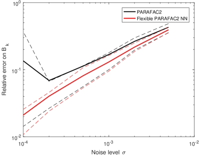
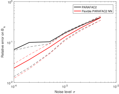
To study robustness to initialization, Figure 1 exhibits the error on $B_{k}$ with both one random initialization and the best out of five initializations.

Figure 1: Relative error on $B_{k}$ for one initialization (left) and best of five initializations (right), showing in dotted lines the 20% and 80% quantiles.

From the results shown in Figure 1, it can be concluded that, for the specific choice of shifted coupled factor $B_{k}$, the flexible PARAFAC2 best performance is similarly to the state-of-the-art PARAFAC2 algorithm best performance, with slightly lower estimation error due to the nonnegativity constraints applied on the $B$ factor. Also, the average performances are significantly better for the flexible PARAFAC2, and the worst results are also much closer to the best ones. Therefore, it seems that the flexible algorithm is more robust to random initializations.

6 Experiments on chromatography data

To further asses the performance of the proposed flexible PARAFAC2 model with nonnegativity constraints, a Gas Chromatography Mass Spectroscopy interval is deconvolved, for which the usual PARAFAC2 model produces poor results. The data come from an analysis of various types of red wine of the type Cabernet Sauvignon. The analysis was done using headspace GC–MS analysis on a Hewlett Packard 6890 GC coupled with an Agilent (Santa Clara, California, United States) 5973 Mass Selective Detector. More details can be found in the publication by Ballabio et al [2].

The chosen interval is difficult to decompose since there is supposedly a double peak in the time elution factors, meaning that the columns of the $B_{k}$ factor are highly colinear. The rank is expected to be either 3 or 4, so that both values were used in the comparisons below. Initial factors for the PARAFAC2 decompositions were drawn from uniform distributions on [0,1]. We picked the best results out of ten runs for both the unconstrained and flexible PARAFAC2 algorithms, based on the reconstruction error.

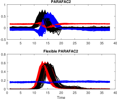
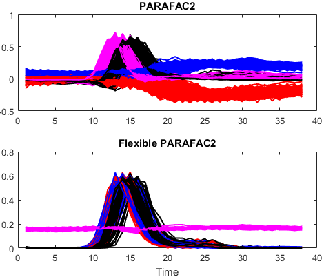
Results are presented in Figure 2. First it can be observed that the elution profiles obtained using PARAFAC2 and flexible PARAFAC2 with nonnegativity constraints are different. Only the flexible PARAFAC2 outputs make sense in terms of elution profiles, for both three and four components models. Moreover, the flexible PARAFAC2 model identifies a very faint third peak in the elution profiles for a four components model, which is not properly detected by the PARAFAC2 model without nonnegativity constraints. This means that the nonnegative flexible PARAFAC2 model has the ability to produce solutions to some problems the PARAFAC2 model could not solve. It is important to note, however, that for most other intervals that we studied, both algorithms performed similarly.

Figure 2: Elution profiles obtained by (top) PARAFAC2 and (bottom) Flexible PARAFAC2 with nonnegativity constraints. The rank is set to (left) 3 and (right) four.

7 Conclusion

The difficult problem of imposing nonnegative constraints on the coupled mode in the PARAFAC2 model is tackled in this manuscript. Using a flexible coupling formalism, the coupled variables and their latent representation are split, which leads to a simple constrained alternating least squares algorithm that is easily shown to converge for fixed regularization parameters. Through the decomposition of both simulated and gas chromatography mass spectroscopy data, it is shown that the proposed flexible PARAFAC2 model behaves at worse similarly to the state-of-the-art PARAFAC2 model, but implementing nonnegativity constraints on all modes and featuring more robustness to random initialization. Further works will focus on a more precise analysis of the flexible PARAFAC2 model for solving various problems, and an extension for imposing any off-the-shelf constraints on the coupled mode.

8 Acknowledgements

The authors wish to thank Nicolas Gillis for helpful discussions on alternatives to the flexible coupling approach for computing nonnegative PARAFAC2.

References

- [1] J. M. Amigo, T. Skov, R. Bro, J. Coello, and S. Maspoch. Solving GC-MS problems with PARAFAC2. TrAC Trends in Analytical Chemistry, 27(8):714–725, 2008.
- [2] D. Ballabio, T. Skov, R. Leardi, and R. Bro. Classification of gc-ms measurements of wines by combining data dimension reduction and variable selection techniques. Journal of chemometrics, 22(8):457–463, 2008.
- [3] R. Cabral Farias, J. E. Cohen, and P. Comon. Exploring multimodal data fusion through joint decompositions with flexible couplings. IEEE Transactions on Signal Processing, 64(18):4830–4844, 2016.
- [4] P. Comon, X. Luciani, and A. LF. De Almeida. Tensor decompositions, alternating least squares and other tales. Journal of chemometrics, 23(7-8):393–405, 2009.
- [5] I. García, L. Sarabia, M. C. Ortiz, and J. M. Aldama. Building robust calibration models for the analysis of estrogens by gas chromatography with mass spectrometry detection. Analytica chimica acta, 526(2):139–146, 2004.
- [6] N. Gillis and F. Glineur. Accelerated multiplicative updates and hierarchical ALS algorithms for nonnegative matrix factorization. Neural Computation, 24(4):1085–1105, 2012.
- [7] R. A Harshman. PARAFAC2: Mathematical and technical notes. UCLA working papers in phonetics, 22(3044):122215, 1972.
- [8] R. A Harshman, S. Hong, and M. E Lundy. Shifted factor analysis—part I: Models and properties. Journal of chemometrics, 17(7):363–378, 2003.
- [9] L. G. Johnsen, P. B Skou, B. Khakimov, and R. Bro. Gas chromatography–mass spectrometry data processing made easy. Journal of Chromatography A, 1503:57–64, 2017.
- [10] H.AL. Kiers, J.MF Ten Berge, and R. Bro. PARAFAC2-part I. A direct fitting algorithm for the PARAFAC2 model. Journal of Chemometrics, 13(3-4):275–294, 1999.
- [11] M. Mørup, LK. Hansen, SM. Arnfred, L-H. Lim, and KH. Madsen. Shift-invariant multilinear decomposition of neuroimaging data. NeuroImage, 42(4):1439–1450, 2008.
- [12] F. Pompili, N. Gillis, P-A. Absil, and F. Glineur. Two algorithms for orthogonal nonnegative matrix factorization with application to clustering. Neurocomputing, 141:15–25, 2014.
- [13] T. Skov and R. Bro. A new approach for modelling sensor based data. Sensors and Actuators B: Chemical, 106(2):719–729, 2005.
- [14] B. M. Wise, N. B. Gallagher, and E. B. Martin. Application of PARAFAC2 to fault detection and diagnosis in semiconductor etch. Journal of chemometrics, 15(4):285–298, 2001.