vh@nnlo-v2: New physics in Higgs Strahlung

Abstract

Introducing version 2 of the code vh@nnlo [1], we study the effects of a number of new-physics scenarios on the Higgs-Strahlung process. In particular, the cross section is evaluated within a general 2HDM and the MSSM. While the Drell-Yan-like contributions are consistently taken into account by a simple rescaling of the SM result, the gluon-initiated contribution is supplemented by squark-loop mediated amplitudes, and by the $s$-channel exchange of additional scalars which may lead to conspicuous interference effects. The latter holds as well for bottom-quark initiated Higgs Strahlung, which is also included in the new version of vh@nnlo. Using an orthogonal rotation of the three Higgs CP eigenstates in the 2HDM and the MSSM, vh@nnlo incorporates a simple means of CP mixing in these models. Moreover, the effect of vector-like quarks in the SM on the gluon-initiated contribution can be studied. Beyond concrete models, vh@nnlo allows to include the effect of higher-dimensional operators on the production of CP-even Higgs bosons. Transverse momentum distributions of the final state Higgs boson and invariant mass distributions of the $V\!\phi$ final state for the gluon- and bottom-quark initiated contributions can be studied. Distributions for the Drell-Yan-like component of Higgs Strahlung can be included through a link to MCFM. vh@nnlo can also be linked to FeynHiggs and 2HDMC for the calculation of Higgs masses and mixing angles. It can also read these parameters from an SLHA-file as produced by standard spectrum generators. Throughout the manuscript, we highlight new-physics effects in various numerical examples, both at the inclusive level and for distributions.

1 Introduction

With the ongoing Run II of the Large Hadron Collider (LHC), more and more properties of the Higgs boson $H$ with mass $125$ GeV, discovered in 2012 [2, 3], are determined with increasing precision [4, 5]. An important process in this respect is Higgs Strahlung, i.e. the production of the Higgs boson in association with a gauge boson $V$, which was used recently to access for the first time the decay rate $H\to b\bar{b}$ [6, 7], for example.

At tree-level, Higgs Strahlung is initiated through light quarks (Drell-Yan (DY)-like contribution). At ${\cal O}(\alpha_{s}^{2})$, a loop-induced, gluon-initiated contribution enters $Z\!H$ production which is particularly sensitive to new-physics effects such as modified Yukawa couplings, new particles in the loop, or resonant additional Higgs bosons. In extended Higgs sectors, also the bottom-quark initiated tree-level sub-process may become important for $Z\!H$ production.

In order to study such new-physics effects at the level of total as well as differential cross sections, we extend the code vh@nnlo [8], which in its previous public release only included Higgs Strahlung within the Standard Model (SM). The main purpose of vh@nnlo so far was the efficient calculation of the total cross section for Higgs Strahlung including next-to-next-to-leading order (NNLO) quantum chromodynamics (QCD) [9, 10] and next-to-leading order (NLO) electro-weak effects [11]. The NNLO QCD corrections to the DY-like terms were calculated by employing ZWPROD’s implementation of the total NNLO Drell-Yan cross section [12]. Soft-gluon resummation effects are small compared to the NNLO fixed-order result [13], which indicates a good convergence of the perturbative series. The SM electro-weak effects to the DY-like terms are implemented in terms of numerical tables, obtained from Ref.[11]. Also included are contributions to DY-like production involving a closed fermion loop, first calculated in Ref.[14] (see Sect. 2.2 for details). The gluon-initiated contribution $gg\to Z\!H{}$ was originally implemented with the help of FeynArts [15] and FormCalc [16] at the level of squared amplitudes. The current implementation, on the other hand, is at the level of amplitudes: For the SM, the 2-Higgs-Doublet Model (2HDM), and Minimal Supersymmetric Standard Model (MSSM), we use the result of Kniehl and Palisoc [17]; other new-physics effects have been taken into account with the help of FormCalc. For the SM, the calculation of the gluon-initiated contribution is supplemented by the NLO QCD $K$-factor as described in Ref.[18]. Ref.[19] discussed the resummation of threshold effects for $gg\to Z\!H{}$ in the SM, which reduce the scale uncertainty substantially; they are not included in the current version of vh@nnlo though.

As already reported in Ref.[20], vh@nnlo has been extended to study Higgs Strahlung $pp\to W\!\phi$/$Z\!\phi{}$ in a general 2HDM, one of the simplest extensions of the SM Higgs sector, see Refs.[21, 22, 23, 24, 25, 26]. Assuming the absence of tree-level flavor-changing neutral currents and CP violation, the two Higgs doublets form three physical, neutral Higgs bosons $\phi$: two CP-even Higgs bosons $h$ and $H^{0}$ with $m_{h}<m_{H^{0}}$ and one CP-odd Higgs boson $A$. The different ways to couple the two Higgs doublets to fermions imply four types of 2HDMs (see Ref.[20], for example). A brief report on Higgs Strahlung within the 2HDM is contained in Ref.[27]; more detailed studies can be found in Refs.[20, 28]. The DY-like contribution to the cross section in the 2HDM can simply be obtained from the SM result by re-weighting with the corresponding $VV\phi$ couplings. The gluon-initiated contribution, on the other hand, also depends on the Yukawa couplings. Moreover, with an increased bottom-quark Yukawa coupling, the bottom-quark initiated contribution, where the final state Higgs $\phi$ couples directly to the initial state bottom-quarks, is of relevance. In addition, both latter processes involve contributions from the $s$-channel exchange of a (resonant or virtual) scalar $\phi^{\prime}\neq\phi$, which may alter the cross section decisively. The program vh@nnlo takes them into account, including all interferences. While these statements also hold for the MSSM, the latter involves additional effects in the gluon-initiated component due to squark-loops [29, 30, 31, 32, 33, 34, 17], albeit only for $Z\!A$ production. The current release of vh@nnlo includes those as well. Furthermore, both in the 2HDM and the MSSM, vh@nnlo allows for a mixing of the Higgs CP eigenstates to three neutral mass eigenstates.

The implementation of the $gg\to Z\phi$ component at the amplitude level clearly facilitates the inclusion of new-physics effects in vh@nnlo. Therefore, aside from the 2HDM and the MSSM, the new version of vh@nnlo currently also includes vector-like quarks (VLQs) and effective Higgs couplings through dimension-6 operators. The latter were checked successfully against earlier work in the framework of MadGraph [35, 36]. For the former, we follow the general parametrization of Ref.[37] of the seven relevant representations of the VLQs.

Whereas most of our discussion aims at the prediction of the inclusive cross section for Higgs Strahlung, our implementation of the $gg\to Z\phi{}$ and the $b\bar{b}\to Z\phi{}$ components also allows for differential quantities such as the Higgs boson’s transverse momentum ($p_{T}$), and the $Z\!H{}$ invariant mass distribution. Within the SM, fully differential predictions for Higgs Strahlung at NNLO QCD were provided in Ref.[38, 39, 40]. NLO electro-weak effects were calculated in Ref.[41]. New-physics effects on the boosted regime ($p_{T}^{H}\gtrsim 150$ GeV) for the gluon-initiated contribution were first discussed in Ref.[42, 43, 20]. In order to allow for the prediction of kinematical distributions for all sub-contributions to Higgs Strahlung, the new release of vh@nnlo provides a link to MCFM [44, 45, 46, 47].

The paper is organized as follows: We start with an outline of the Higgs-Strahlung process and its partonic sub-processes as they are implemented in vh@nnlo in Sect. 2. Section 3 describes the generic settings of vh@nnlo which are relevant for every run of vh@nnlo. Section 4 focuses on how to obtain kinematic distributions in vh@nnlo. In Sect. 5, we address the newly implemented new-physics scenarios and consider their numerical effects through various examples. Sect. 6 contains our conclusions. Details about the installation and compilation of the code can be found in Appendix A, and options for links to external codes are described in Appendix B.

2 General structure and Standard Model mode

2.1 Contributions to the cross section

The implementation of the total inclusive cross section for Higgs Strahlung in vh@nnlo has the form

$$\sigma^{V\!\phi{}}=(1+\delta_{\text{{EW}}}^{V\!\phi})\sigma_{\text{{DY}}{}}^{V\!\phi{}}+\sigma_{\rm I}^{V\!\phi{}}+\delta_{V\!Z}\left(\sigma_{\rm II}^{Z\!\phi{}}+K^{\infty}_{\text{{NLO}}}\sigma_{gg\to Z\phi{}}+\sigma_{b\bar{b}\to Z\phi{}}\right)\,,$$ (1)

where $\sigma_{\text{{DY}}{}}^{V\!\phi{}}$ denotes the DY-like terms, whose leading order diagram is shown in Fig. 1 (a). By definition, we only count diagrams as DY-like if they can be obtained from Fig. 1 (a) by dressing it with real or virtual gluons and quarks via strong interactions, and possibly crossing them between the initial and final state. Consequently, the structure of the QCD corrections to $\sigma_{\text{{DY}}{}}^{V\!\phi{}}$ is the same for both $W\!\phi{}$ and $Z\!\phi{}$ production; it is determined by the QCD corrections to the DY process $q^{\prime}\overline{q}\to V^{*}$, provided through NNLO in Ref.[12] (see Ref.[10] for details). The other terms in Eq. (1) will be discussed in more detail in subsequent parts of this paper.

2.2 Standard Model cross section

In the SM mode of vh@nnlo, all terms shown in Eq. (1) can be included. All but the first and the last one only contribute at NNLO QCD and beyond, i.e. at $\mathcal{O}(\alpha_{s}^{2})$, and involve loops of top- or bottom-quarks. Eq. (1) assumes that electro-weak effects $\delta_{\text{{EW}}}^{V\!\phi}$ [11, 41] to the DY-like contribution fully factorize from the QCD effects. The term $\sigma_{\rm I}^{V\!H{}}$ is similar for $W\!H{}$ and $Z\!H{}$ production and involves diagrams where a top-quark loop is inserted into a gluon line of the real and virtual NLO QCD diagrams to $pp\to V^{*}$, from which the Higgs boson is radiated. The effect of these contributions on the inclusive cross section is at the 1–2% level [14]. The contribution $\sigma_{\rm II}^{Z\!H{}}$, which only exists for $Z\!H{}$ production, represents $q\bar{q}$-induced diagrams where the $Z$ boson couples to a closed top- or bottom-quark loop. Its contribution on the total rate is even smaller than $\sigma_{\rm I}^{V\!H{}}$ [14]. We will refer to the latter two contributions collectively as $\sigma_{\text{I+II}}^{V\!H}$ in what follows.

Much more relevant for $Z\!H{}$ production is the gluon-initiated contribution $\sigma_{gg\to Z\!H{}}$, whose generic LO diagrams are displayed in Figs. 1 (b) and (c). Here, a closed fermion loop is connected to two initial state gluons and the $Z$ boson is attached to this loop, whereas the Higgs boson $H$ is either radiated off the $Z$ boson or off the closed fermion loop, leading to triangle and box diagrams, respectively. It is well known that these two contributions interfere destructively in the SM [48, 49]. Ref.[18] provided the NLO QCD $K$-factor for the $gg\to Z\!H$ sub-process in the heavy-top limit, denoted $K^{\infty}_{\text{{NLO}}}$ in Eq. (1), which enhances this contribution by roughly a factor of two. Corrections beyond the strict heavy-top limit were calculated in Ref.[50], and Ref.[19] supplied the soft-gluon resummation which leads to a decrease of the residual renormalization scale dependence. As pointed out in Sect. 1, the current implementation of $\sigma_{gg\to Z\phi{}}$ in vh@nnlo uses the results of Ref.[17] and the NLO $K$-factor of Ref.[18], as well as new-physics amplitudes obtained with FormCalc [16]. Soft-gluon resummation [19] is currently not included.

Eq. (1) involves two bottom-quark initiated contributions. The first one is contained in $\sigma_{\text{\text{{DY}}}}^{V\!\phi}$ and depends only on the gauge couplings of the bottom quarks. The second one, $\sigma_{b\bar{b}\to Z\phi}$, is proportional to the bottom Yukawa coupling; sample diagrams which contribute to the latter in the SM are shown in Fig. 2 (a) and (b). Currently, $\sigma_{b\bar{b}\to Z\phi}$ is implemented only at LO QCD. Since we assume the initial-state bottom-quarks to be massless (while keeping the Yukawa coupling non-zero), there is no interference between $\sigma_{b\bar{b}\to Z\phi}$ and $\sigma_{\text{\text{{DY}}}}^{V\!\phi}$. The numerical effect of $\sigma_{b\bar{b}\to Z\phi}$ becomes important in certain models beyond the SM (BSM), see below.

In vh@nnlo, each of the terms in Eq. (1) is provided separately for the total inclusive cross section, as will be explained in more detail in Sect. 3.

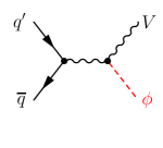
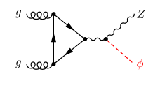
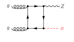
(a)	(b)	(c)

Figure 1: Leading-order Feynman diagrams to $\sigma^{V\!\phi{}}$, see Eq. (1): (a) DY-like terms $\sigma_{\text{\text{{DY}}}}^{V\!\phi}$, (b,c) gluon-initiated contribution $\sigma_{gg\to Z\phi}$.

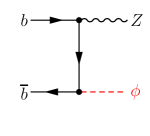
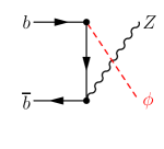
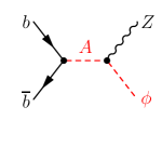
(a)	(b)	(c)

Figure 2: Feynman diagrams for bottom-quark initiated Higgs Strahlung, $\sigma_{b\bar{b}\to Z\phi}$.

3 Generic options of vh@nnlo

In this section we focus on the basic input for a generic vh@nnlo run. The installation of the code is described in Appendix A. The code itself can be downloaded from Ref.[1].

Compared to version 1.0, vh@nnlo has significantly extended its functionality and capability. This implies an extended set of input parameters. The input of vh@nnlo is controlled through SLHA-inspired input blocks (see Refs.[51, 52]). We begin with the description of the blocks VERSION, VHATNNLO, ORDER, SCALES, PDFSPEC, and SMPARAMS, which define the central parameters for each run of vh@nnlo and need to be part of all input files. The settings are summarized in Tables 1–7. In these tables and throughout the draft, the notation NAME($i$)=$k$ means that the entry $i$ of Block NAME is set to $k$.

For all input blocks which are required in the SM mode (i.e. VHATNNLO(1)=0), vh@nnlo provides default entries which are automatically set if the corresponding entry in the input file is missing. Their values are specified in Tables 1–7 and 10. In contrast, blocks which specify new physics do not provide default values, except for a few documented cases. The units of the input parameters are given in square brackets in the column “meaning” of these tables. All dimensionful quantities are of data type “real”. For input values of data type “integer”, the table lists the set of allowed values in column “range”. Since such restrictions are much more difficult to define for most of the input parameters of type “real”, we refrain from any explicit restrictions in this case and appeal to the user’s common sense when setting these parameters.

In order to check the consistency of the input file with the version of vh@nnlo, the user needs to provide the version number in VERSION(1). Accordingly, input files of version 1.0 of vh@nnlo will not run with the current version 2. The entries $1$ and $2$ of Block VHATNNLO define the model and the Higgs boson type assumed in the calculation. In the 2HDM or the MSSM, VHATNNLO(2)=11/12/21 selects $h/H^{0}/A$ as the final-state Higgs boson, respectively. The only allowed setting for the SM mode (VHATNNLO(1)=0) is 11. Entries $3$ and $4$ of Block VHATNNLO determine the type of collider ($pp$ or $p\bar{p}$) and its center-of-mass energy. VHATNNLO(5) specifies the vector boson in the final state ($Z\phi$, $W^{+}\phi$, $W^{-}\phi$, or $(W^{+}+W^{-})\phi$). Finally, VHATNNLO(6) allows to reduce/enhance the screen output of vh@nnlo.

Block VERSION
entry	default	meaning
1	2.0	version of vh@nnlo

Table 1: Settings of Block VERSION.

Block VHATNNLO
entry	default	range	meaning
1	0	{0,1,2}	{SM, MSSM, 2HDM} — model
2	11	{11,12,21}	{SM/$h$, $H$, $A$} — Higgs type
3	1	{1,2}	{$pp$, $p\bar{p}$} — collider type
4	1.3d4		$\sqrt{s}$ [GeV] — collider energy
5	1	{0,1,2,3}	{$W^{+}+W^{-}$, $Z$, $W^{-}$, $W^{+}$}$\phi$ — final state
6	1	{0,1}	{quiet, verbose}

Table 2: Basic run parameters of vh@nnlo.

Block ORDER controls the inclusion of the various sub-contributions to Higgs Strahlung and their corresponding order in perturbation theory. ORDER(1)=0/1/2 determines the order of the DY-like terms, LO/NLO/NNLO; ORDER(1)=-1 switches them off. The other sub-processes are unaffected by this setting. Note that the order of the running of $\alpha_{s}$ for all processes is always determined by the order of the PDF set defined in Block PDFSPEC. The $gg\to Z\!H$ component is controlled by ORDER(2): setting it to 0 or 1 includes it at LO or NLO, i.e. ${\cal O}(\alpha_{s}^{2})$ or ${\cal O}(\alpha_{s}^{3})$, respectively, while ORDER(2)=-1 switches it off. The additional top-quark induced terms $\sigma_{\rm I}^{V\!H{}}$ and $\sigma_{\rm II}^{Z\!H{}}$ are disabled/enabled by setting ORDER(3)=-1/0, the bottom-quark induced contribution $b\bar{b}\to Z\phi{}$ by ORDER(4)=-1/0, and the electro-weak correction factor $\delta_{\text{EW}}^{V\!H{}}$ by ORDER(5)=-1/0. We note that the settings ORDER(2)=1 and ORDER(3,5)=0 are only allowed in the SM. The entry ORDER(10)=-1/0 toggles $\Delta_{b}$ resummation in the bottom-Yukawa coupling for $\tan\beta$-enhanced sbottom contributions, in case the link to FeynHiggs is active. We refer to Sect. 5.2 for details.

By default, the renormalization and factorization scale ($\mu_{\text{R}}$, $\mu_{\text{F}}$) is set relative to the invariant mass of the $V\!\phi$ system through the entries SCALES(1,2), respectively. This means that these scales vary with the integration variable $\hat{s}$ when convolving the partonic cross section with the parton densities. With the exception of the DY-like terms, $\mu_{\text{R}}$ and $\mu_{\text{F}}$ can also be fixed in absolute terms to the values given in SCALES(3,4), respectively, by setting SCALES(10)=1. The DY-terms must be switched off in this case, i.e. ORDER(1)=-1.

PDFSPEC(1) sets the name of the employed parton distribution function (PDF), see Table 5. Since vh@nnlo needs to be linked to LHAPDF [53], all PDF sets of LHAPDF can be loaded. For each run, only one PDF set can be specified, which will be used throughout the calculation of all sub-processes. PDFSPEC(10) fixes the PDF set number. vh@nnlo will automatically use the value of $\alpha_{s}(M_{Z})$ which corresponds to the specified PDF set for the calculation of the partonic cross section.

Block ORDER
entry	default	range	meaning
2	1	{-1,0,1,2}	$n$ — include $\sigma_{\text{{DY}}}^{V\!\phi}$ at order $\alpha_{s}^{n}$ (-1=off)
3	1	{-1,0,1}	$n$ — include $\sigma_{gg\to Z\phi}$ at order $\alpha_{s}^{n+2}$ (-1=off)
4	1	{-1,0}	include $\sigma_{\text{I+II}}^{V\!H}$: {no, yes}
5	1	{-1,0}	include $\sigma_{b\bar{b}\to Z\phi}$: {no, yes}
6	1	{-1,0}	include $\delta_{\text{{EW}}}^{V\!\phi}$: {no, yes}
10	1	{-1,0}	include $\Delta_{b}$ resummation: {no, yes}

Table 3: Controlling the sub-contributions defined in Eq. (1).

Block SCALES
entry	default	range	meaning
1	1.		renormalization scale $\mu_{\text{R}}/M_{V\!\phi}$
2	1.		factorization scale $\mu_{\text{F}}/M_{V\!\phi}$
3	125.		fixed $\mu_{\text{R}}$ [GeV]
4	125.		fixed $\mu_{\text{F}}$ [GeV]
10	0	{0,1}	define $\mu_{\text{R}}$ and $\mu_{\text{F}}$ relative to $M_{V\!\phi}$: {yes, no}; if=0, use SCALES(1 and 2); if=1, use SCALES(3 and 4)

Table 4: Defining the unphysical scales. $M_{V\!\phi}$ is the invariant mass of the $V\!\phi$ system.

Block PDFSPEC
entry	default	meaning
1	’PDF4LHC15_nnlo_mc.LHgrid’	PDF set name (from LHAPDF)
10	0	PDF set number

Table 5: Choosing a PDF set.

Block MASS
entry	default	meaning
25	125.	Higgs mass (in the SM) [GeV]

Table 6: Setting the Higgs mass in the SM. For the 2HDM and the MSSM, see Table 12.

Block SMPARAMS
entry	default	meaning
2	1.16637d-5	Fermi’s constant $G_{F}$ [GeV-2]
3	0.118	$\alpha_{s}(M_{Z})$ [used by FeynHiggs/2HDMC]
4	91.1876	$Z$-boson mass $M_{Z}$ [GeV]
5	4.18	$\overline{\mbox{{MS}}}$ $b$ mass $m_{b}(m_{b})$ used by FeynHiggs/2HDMC,
		as well as $b\bar{b}\to Z\phi$ [GeV]
6	172.5	on-shell $t$ mass [GeV]
10	4.92	on-shell $b$ mass [GeV]
11	80.385	$W$-boson mass $M_{W}$ [GeV]
12	2.4952	$Z$-boson width $\Gamma_{Z}$ [GeV]
13	2.085	$W$-boson width $\Gamma_{W}$ [GeV]
14	0.05077	Cabbibo angle $\sin^{2}\theta_{C}$

Table 7: Setting the SM input parameters.

Block MASS defines the masses of the Higgs bosons of the theory by employing the corresponding PDG codes; in the SM mode, only MASS(25) is relevant. If run with FeynHiggs or 2HDMC, this block is overwritten though, see Sect. 5.1 and Sect. 5.2. In this case, the output file will also list the total decay widths of the $h/H/A$ boson in MASS(250/350/360) as calculated by these external programs.

The block SMPARAMS defines numerical values for the central SM parameters. SMPARAMS(2) sets the numerical value for Fermi’s constant. SMPARAMS(3) allows to provide a value for $\alpha_{s}(M_{Z})$ which is independent of the one associated with the PDF set specified in Block PDFSPEC, see below. It will only be used by FeynHiggs or 2HDMC, however; the partonic cross section is always calculated using the value of $\alpha_{s}(M_{Z})$ as taken from the employed PDF set. In entries 6,10,5,4,11 of Block SMPARAMS, the masses of the top-quark, the bottom-quark (on-shell and $\overline{\mbox{{MS}}}{}$ $m_{b}(m_{b})$), the $Z$-boson and the $W$-boson are defined, respectively. The on-shell bottom-quark mass $M_{b}$ is used to define the SM Yukawa coupling $Y_{b}^{\text{OS}}=M_{b}/v$ in the $gg\to Z\phi$ process, and also enters the associated loop integrals. The $\overline{\mbox{{MS}}}{}$ bottom-quark mass, on the other hand, enters as input for FeynHiggs, 2HDMC, and the sbottom-Higgs couplings, see Sects. 5.1 and 5.2. For the Yukawa coupling $Y_{b}=m_{b}(\mu_{\text{R}})/v$ which occurs in $b\bar{b}\to Z\phi{}$, $m_{b}(\mu_{\text{R}})$ is obtained from $m_{b}(m_{b})$ through four-loop renormalization group running. SMPARAMS(12,13) contain the total widths of the gauge bosons. vh@nnlo internally calculates the weak mixing angle from $\sin^{2}\theta_{W}=1-M_{W}^{2}/M_{Z}^{2}$, and the fine structure constant from $\alpha=G_{F}\sqrt{2}M_{W}^{2}\sin^{2}\theta_{W}/\pi$, which are listed in entries 15 and 1 of Block SMPARAMS in the output file, respectively. Finally, the Cabbibo angle is specified in SMPARAMS(14). It enters the calculation of the DY-like terms and top-quark induced contributions.

Block FACTORS
entry	default	meaning
1	1.0	factor for $ht\bar{t}$ coupling
2	1.0	factor for $hb\bar{b}$ coupling
3	1.0	factor for $hVV$ coupling
111	entry 1	factor for $ht\bar{t}$ coupling
211	entry 2	factor for $hb\bar{b}$ coupling
311	entry 3	factor for $hVV$ coupling
121	entry 1	factor for $At\bar{t}$ coupling
221	entry 2	factor for $Ab\bar{b}$ coupling
321	entry 3	factor for $AVV$ coupling
112	entry 1	factor for $Ht\bar{t}$ coupling
212	entry 2	factor for $Hb\bar{b}$ coupling
312	entry 3	factor for $HVV$ coupling

Table 8: Modifying the Higgs couplings.

Another potential input block available in all models is Block FACTORS which allows to alter the couplings of all involved Higgs bosons to quarks and gauge bosons. The user can either specify common factors identical for all Higgs bosons through entries 1–3 for the couplings to the top quark, the bottom quark and the gauge bosons, respectively. Alternatively, the entries {111, 211, 311}, {112, 212, 312} and {121, 221, 321} separately change the couplings of the light Higgs boson, the heavy Higgs boson and the pseudoscalar, respectively (see Table 8). If not specified, these entries are replaced by their default value ($=1.0$). The $AhZ$ and $AHZ$ coupling of the 2HDM and the MSSM (see Eq. (3) below) are re-scaled in the same way as the $VVH$ and the $VVh$ couplings, respectively. Note that, since currently vh@nnlo always assumes a vanishing $VVA$ coupling in accordance with a 2HDM with real parameters, FACTORS(321)is ineffective at the moment. The couplings of the CP-even scalars to squarks are currently fixed to their values determined by SUSY and cannot be changed.

Finally, Block VEGAS allows to control the numerical integration parameters, separately for the DY-like, the gluon initiated, and bottom-quark initiated contributions. More details on this block can be found in Appendix B.1.

Before discussing the new-physics input, we shortly explain the output file vh.out of vh@nnlo. It contains all input blocks, partially extended by parameters calculated internally. In addition, Block MASS and Block HIGGSCOUP provide information about the Higgs mass(es), their widths (if calculated by 2HDMC or FeynHiggs) as well as its/their coupling(s) to third generation quarks and gauge bosons. Block SIGMA summarizes the calculated production cross section, split into the individual sub-processes, including the integration errors. Its entries are presented in Table 9. The total cross section presented in SIGMA(1) is calculated according to Eq. (1). Block SIGMA also includes the value of $\alpha_{s}(M_{Z})$ associated with the employed PDF set.

Block SIGMA
entry	example	meaning
1	8.68271087E-01	total cross section $\sigma^{V\!\phi}$ [pb]
111	2.31607286E-03	integration error on $\sigma^{V\!\phi}$ [pb]
10	1.18002301E-01	$\alpha_{s}(M_{Z})$ (from PDF set)
11	7.93648481E-01	$\sigma_{\text{{DY}}}^{V\!\phi}$ [pb] (without $\delta_{\rm EW}^{V\!H}$)
110	2.32596191E-03	integration error on $\sigma_{\text{{DY}}}^{V\!\phi}$ [pb]
12	9.47250000E-01	$1+\delta_{\rm EW}^{V\!H}$
13	5.14585867E-02	$\sigma_{gg\to Z\phi}$ [pb] (without $K^{\infty}_{\text{{NLO}}}$)
130	3.42836009E-04	integration error on $\sigma_{gg\to Z\phi}$ [pb]
14	2.07452931E+00	$K$-factor for $gg\to Z\!H$, $K_{\text{{NLO}}}^{\infty}$
15	4.31358140E-04	$\sigma_{b\bar{b}\to Z\phi}$ [pb]
150	7.04767054E-07	integration error on $\sigma_{b\bar{b}\to Z\phi}$ [pb]
16	9.30486135E-03	$\sigma_{\text{I+II}}^{V\!H}$ [pb]
160	6.30595571E-05	integration error on $\sigma_{\text{I+II}}^{V\!H}$ [pb]

Table 9: Results presented in Block SIGMA.

4 Kinematic distributions

Fully differential predictions for the Higgs Strahlung process within the SM through NNLO QCD have been available for some time [38, 39, 40]. Since recently, they are also publicly available in MCFM [44, 45, 46, 47]. Since the new-physics effects discussed here affect the DY-like component of the Higgs-Strahlung process only through a global factor, we link MCFM to vh@nnlo and rescale this component accordingly. The kinematic distributions of the $gg\to Z\phi$ and $b\bar{b}\to Z\phi{}$ components are calculated within vh@nnlo at LO QCD, including all available new-physics effects. Here, one can choose between $p_{T}$ or $M_{V\!\phi{}}$ distributions, where $p_{T}$ denotes the transverse momentum of the Higgs boson, and $M_{V\!\phi{}}$ is the invariant mass of the $V\phi$ system.

Block DISTRIB
entry	default	range	meaning
1	1	{1,2}	distribution type: {$p_{T}$, $M_{V\!\phi{}}$}
2	0.		minimal value of distribution parameter [GeV]
3	1000.		maximal value of distribution parameter [GeV]
4	10.		bin width [GeV]
5	0	{0,1}	run with MCFM: {no, yes}
6	0	{0,1}	calculate $gg\to Z\!H{}$ distribution in the SM: {no, yes}
7	’undefined’		read histogram from MCFM output file (character)
8	0.		minimal invariant mass $M_{V\!H{}}$ for MCFM [GeV]
9	$\sqrt{s}$		maximal invariant mass $M_{V\!H{}}$ for MCFM [GeV]
10	10		iterations with VEGAS for MCFM
11	10000		number of calls per iteration for MCFM

Table 10: Setting the parameters for kinematical distributions.

If the input file contains a Block DISTRIB (see Table 10), vh@nnlo produces a kinematic distribution which is written to the file ptDist_’outputfile’ or mhvDist_’outputfile’, where outputfile is the name of the output file, see Appendix A for details. The prefix of the file name depends on the distribution type selected in DISTRIB(1). Block DISTRIB also allows to set a minimal and maximal value for the kinematic variable under consideration in DISTRIB(2/3) (histo start/histo end), together with the bin width in DISTRIB(4). Unless vh@nnlo is linked to MCFM, the kinematical distribution only includes the contributions from $gg\to Z\phi$ and $b\bar{b}\to Z\phi$ (listed separately). We emphasize that, rather than integrating the distributions within each bin, vh@nnlo directly evaluates the distributions $d\sigma/dp_{T}$ or $d\sigma/dM_{V\!\phi{}}$ for these contributions at the center of the specified bins. The DY-like contribution requires a link to MCFM and, if established, is shown in a third column, potentially rescaled by the couplings of the specified BSM theory. MCFM needs a number of additional input files to be put in the folder MCFM of the vh@nnlo directory. In order to obtain results which are compatible with the settings of vh@nnlo, the MCFM flags removebr and zerowidth are set to true such that the Higgs and the $W/Z$ bosons do not decay. Fig. 3 shows examples for $p_{T}$ and $M_{V\!H{}}$ distributions produced with MCFM and vh@nnlo in the SM. Two well-known features are visible: The $p_{T}$ distributions of quark- and gluon-induced components show different shapes and peak at different positions in $p_{T}$; the $M_{Z\!H{}}$ distribution of the $gg\to Z\!H$ contribution clearly shows the top-quark threshold at $M_{Z\!H{}}=2m_{t}$.

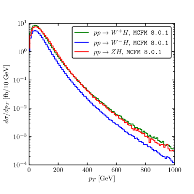
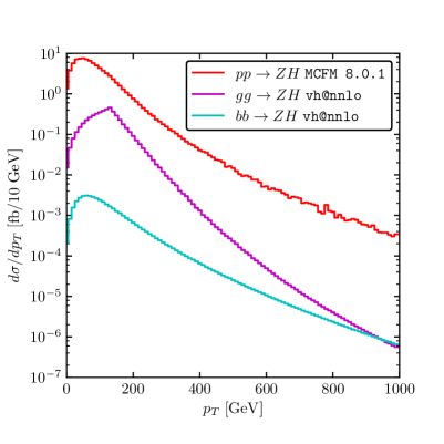
(a)	(b)
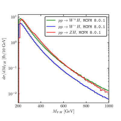
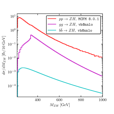
(c)	(d)

Figure 3: Example of transverse momentum distributions in (a) and (b) and invariant mass distributions in (c) and (d) for $V\!H{}$ production in the SM at the LHC with $\sqrt{s}=13\;\mathrm{TeV}$ and $M_{\mathrm{H}}=125\;\mathrm{GeV}$; (a,c) Comparison of $W^{+}H$ (green), $W^{-}H$ (blue) and $Z\!H{}$ production (red) created with MCFM 8.0.1; (b,d) Comparison of full $Z\!H{}$ (red), gluon-induced (magenta) and bottom-induced $Z\!H{}$ (cyan) production. All results are obtained at ${\cal O}(\alpha_{s}^{2})$, apart from $b\bar{b}\to Z\!H{}$ which is calculated at LO.

5 Beyond the Standard Model

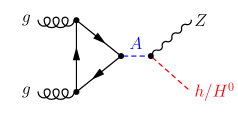
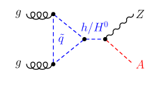
(a)	(b)
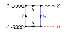
(c)	(d)

Figure 4: Selection of new contributions to the $gg\to Z\phi$ amplitude in the 2HDM/MSSM due to (a) intermediate (pseudo)scalars and (b) squarks in addition; to the $gg\to Z\!H$ amplitude in the SM due to (c) vector-like quarks and (d) dimension-6 operators.

In the following sub-sections we list the different new-physics models and contributions supported by vh@nnlo. A couple of sample diagrams relevant for the $gg\to Z\phi$ contribution are shown in Fig. 4. We start with the 2HDM in Sect. 5.1 including a discussion of resonant (pseudo)scalars, and continue with the MSSM in Sect. 5.2. In both sub-sections we explain the potential links to external codes for the calculation of a consistent set of model parameters. In Sect. 5.3, we address CP mixing among the three neutral 2HDM scalars of these two models. Section 5.4 describes the implementation of vector-like quarks. Finally, in Sect. 5.5 we go beyond a concrete model implementation and describe the incorporation of higher-dimensional operators. Since $\sigma_{\rm I+II}^{V\!H{}}$ as well as the NLO $K$-factor to $gg\to Z\!H{}$ are only known for the SM, they need to be switched off whenever BSM effects are requested. Where appropriate, we discuss numerical examples to highlight the new-physics effects in Higgs Strahlung.

5.1 2-Higgs-Doublet Model

The program vh@nnlo allows to calculate the production cross section for any of the three electrically neutral Higgs bosons in the 2HDM. The effects which distinguish this case from the SM calculation have been described in detail in Ref.[20]. Therefore, they shall be summarized only briefly here. For once, the couplings of the CP-even Higgs bosons to the weak gauge bosons and the quarks are different from the SM Higgs couplings. While the former are the same for all 2HDMs, the Higgs-quark couplings depend on the specific realization of the $\mathbb{Z}_{2}$ symmetry which is imposed in order to avoid tree-level flavor-changing neutral currents. Specifically, for the gauge-Higgs couplings we have

$$\begin{split}g_{VV}^{h}=\sin(\beta-\alpha)\,,\qquad g_{VV}^{H}=\cos(\beta-\alpha)\,,\qquad g_{VV}^{A}=0\,,\qquad V\in\{W,Z\}\,,\end{split}$$ (2)

where $\alpha$ parametrizes the mixing of the CP-even Higgs bosons from the isospin to the mass eigenstates, and $\tan\beta$ is the ratio of the vacuum-expectation values of the two Higgs doublets. The quark-Higgs couplings are summarized in Table 11. In types III and IV, the quark-Higgs couplings equal the ones of types I and II, respectively. Only the couplings to leptons differ; this affects the total widths of the Higgs bosons, and thus indirectly the Higgs-Strahlung cross section through diagrams with Higgs bosons in the $s$-channel.

	$g_{u}^{h}$	$g_{u}^{H}$	$g_{u}^{A}$	$g_{d}^{h}$	$g_{d}^{H}$	$g_{d}^{A}$
Type I	$\cos\alpha/\sin\beta$	$\sin\alpha/\sin\beta$	$\cot\beta$	$\cos\alpha/\sin\beta$	$\sin\alpha/\sin\beta$	$-\cot\beta$
Type II	$\cos\alpha/\sin\beta$	$\sin\alpha/\sin\beta$	$\cot\beta$	$\sin\alpha/\cos\beta$	$\cos\alpha/\cos\beta$	$\tan\beta$

Table 11: The Higgs-quark couplings $g_{f}^{\phi}$ for 2HDM type I and II, see Fig. 5. For types III and IV we refer to the comment in the text.

	$\displaystyle=i\frac{eM_{Z}}{c_{W}s_{W}}g_{VV}^{\phi}g^{\mu\nu}$     $\displaystyle=i\frac{eM_{W}}{s_{W}}g_{VV}^{\phi}g^{\mu\nu}$
	$\displaystyle=-\frac{m_{f}}{v}\{ig_{f}^{h},ig_{f}^{H},g_{f}^{A}\gamma_{5}\}$ for $\phi\in\{h,H,A\}$
	$\displaystyle=\frac{e}{2c_{W}s_{W}}g_{Z}^{A\phi}(p-p^{\prime})^{\mu}$

Figure 5: Feynman rules for the Higgs couplings in the 2HDM. All momenta are ingoing.

Figure 5 and Table 11 also show the couplings of the CP-odd Higgs boson $A$ to quarks. Its coupling to the weak gauge bosons vanishes, but there are tri-linear couplings to $Z\!h{}$ and $Z\!H{}$, also included in Fig. 5, where

$$\begin{split}g_{Z}^{Ah}=\cos(\beta-\alpha)\,,\qquad g_{Z}^{AH}=-\sin(\beta-\alpha)\,.\end{split}$$ (3)

These latter couplings imply new contributions to the Higgs-Strahlung process, with virtual Higgs bosons in the $s$-channel. When Higgs-quark couplings are neglected for the first two quark generations, such contributions can appear only in the partonic processes $b\bar{b}\to Z\phi{}$ and $gg\to Z\phi{}$. Their numerical effects have been studied in detail in Ref.[20]. They can be huge, for example for $gg\to A\to Z\!h{}$ in the wrong-sign limit ($g_{d}^{h}=-1$) of the 2HDM [54]. We note that using Block FACTORS, see Sect. 3, implies that the relative factors of $g_{Z}^{Ah}$ and $g_{Z}^{AH}$ are set to the ones of $g_{VV}^{H}$ and $g_{VV}^{h}$, respectively.

If the mass $M_{\phi^{\prime}}$ of the $s$-channel Higgs boson $\phi^{\prime}$ is larger than the threshold for the $Z\phi$ production process under consideration, the integration over the parton density functions would encounter a pole at $\hat{s}=M^{2}_{\phi^{\prime}}$ which, however, is regulated by the width $\Gamma_{\phi^{\prime}}$ of $\phi^{\prime}$ through the replacement

$$\frac{1}{\hat{s}-m_{\phi^{\prime}}^{2}}\rightarrow\frac{1}{\hat{s}-m_{\phi^{\prime}}^{2}+im_{\phi^{\prime}}\Gamma_{\phi^{\prime}}}\quad.$$ (4)

The numerical value for $\Gamma_{\phi^{\prime}}$ is required by vh@nnlo as input. If FeynHiggs or 2HDMC are linked to vh@nnlo, $\Gamma_{\phi^{\prime}}$ will be taken from their output though. The same effect occurs in the bottom-quark initiated contribution $\sigma_{b\bar{b}\to Z\phi}$ due to Fig. 2 (c). We emphasize that our implementation allows to take into account the interferences of the $s$-channel diagrams $gg/b\bar{b}\to A\to Z\!h{}$ or $gg/b\bar{b}\to\{h,H\}\to Z\!A{}$ with all other Feynman diagrams. Until now, searches for heavy pseudoscalars decaying to $Z\!h{}$ have applied the narrow-width approximation, which means that such interference effects have been neglected. This allowed to include higher-order corrections to the production mechanisms $gg/b\bar{b}\to A$, as implemented in SusHi [55, 56], which can also be linked to 2HDMC to obtain the branching ratio $A\to Z\!h{}$. However, it is well-known from decays of heavy scalars into a pair of gauge bosons $V\!V$ [57, 58] or a pair of Higgs bosons $h\!h$ [59] that interference effects in a 2HDM can be large. Thanks to the option to obtain the invariant mass distribution $M_{Z\!\phi{}}$, vh@nnlo allows to study the shape of the interferences around the mass of the intermediate resonance. We will show an example at the end of this section.

One option to evaluate the cross section in the 2HDM with vh@nnlo is to define the three neutral Higgs boson masses and their total decay widths in Block MASS, see Table 12. The other relevant 2HDM parameters need to be provided in Block 2HDM, also described in Table 12. Recall that various contributions to the cross section can be switched on and off in Block ORDER, see Table 3. Table 11 may serve as definition of $\tan\beta$ and the CP-even Higgs mixing angle $\alpha$ (up to shifts of $\alpha$ by $\pm\pi$, which leave the cross section invariant). As explained before, 2HDM types I and III as well as II and IV have identical quark-Higgs couplings. Thus, using Block 2HDM will reveal identical results for 2HDM(2)=1 and 3 as well as =2 and 4, provided the total Higgs widths are left unchanged.

Block MASS
entry	default	meaning
25	125.	$m_{h}$ [GeV]
35		$m_{H}$ [GeV]
36		$m_{A}$ [GeV]
250		$\Gamma_{h}$ [GeV]
350		$\Gamma_{H}$ [GeV]
360		$\Gamma_{A}$ [GeV]
Block 2HDM
entry	range	meaning
2	{1,2,3,4}	2HDM type I…IV
3		$\tan\beta$
4	see text	CP even Higgs mixing angle $\alpha$

Table 12: Defining the masses and widths of the light and heavy CP even Higgs $h$, $H$, and of the CP-odd Higgs $A$.

Another option to define the 2HDM input parameters is through the link of vh@nnlo to 2HDMC [60, 61] (see Appendix B.3 how to establish the link). If vh@nnlo finds the Block 2HDMC in its input file, it will read 2HDMC input from this block, and ignore the block 2HDM. Linking to 2HDMC gives you access to the features of this program within vh@nnlo, meaning that you can use different parameterizations of the 2HDM, check for theoretical consistency of the 2HDM, and get consistent numerical values for the decay widths of the Higgs particles.

The program 2HDMC produces its own additional output file, named 2HDMC.out, which contains all relevant information about the Higgs spectrum and decay widths. The definition of the entries in Block 2HDMC is described in Table 13. The specific 2HDM parameterization is set by 2HDMC(1), which currently can assume the values 1, 2, and 3, corresponding to the “$\lambda$ basis”, the “physical basis”, and the “$H_{2}$ basis”, respectively (see Refs.[60, 62] for the definition of these bases). The relevant parameters for these bases are given in 2HDMC(11..17), 2HDMC(21..27), and 2HDMC(31..36), respectively. For example, if 2HDMC(1)=1, only 2HDMC(11..17) is used for defining the 2HDM, while 2HDMC(21..27) and 2HDMC(31..36) are ignored. Concerning the Higgs mixing angle $\alpha$, the convention of 2HDMC in the physical and the $H_{2}$ basis assumes $-\tfrac{\pi}{2}\leq\beta-\alpha\leq\tfrac{\pi}{2}$. If the user works with the convention $0\leq\beta-\alpha\leq\pi$, such that $\cos(\beta-\alpha)$ covers the whole range $[-1,1]$ and $\sin(\beta-\alpha)\in[0,1]$, then for values between $\tfrac{\pi}{2}\leq\beta-\alpha\leq\pi$, the 2HDMC convention is obtained by shifting $\beta-\alpha$ by $-\pi$. The other parameters are in principle not constrained, but 2HDMC can check whether a parameter point obeys stability of the vacuum, unitarity and perturbativity requirements. If 2HDMC(10)=1, vh@nnlo will terminate if a 2HDM parameter point does not obey all of these criteria. This is quite useful for large parameter scans. In contrast to the run with Block 2HDM, the link to 2HDMC will reveal differences among the 2HDM types I and III as well as II and IV. This is due to the fact that the decay widths obtained from 2HDMC depend on all couplings, including the Higgs-lepton couplings.

Block 2HDMC
	entry	range	meaning
	1	{1,2,3}	2HDMC input key (basis choice)
	2	{1,2,3,4}	2HDM type {I, II, III, IV}
	3		$\tan\beta$
	4		$m_{12}$ [GeV]
	10	{0,1}	ignore theory inconsistencies: {yes, no}
2HDMC input key	entry		meaning
2HDMC(1)=1	11		$\lambda_{1}$
$\lambda$ basis	12		$\lambda_{2}$
	13		$\lambda_{3}$
	14		$\lambda_{4}$
	15		$\lambda_{5}$
	16		$\lambda_{6}$
	17		$\lambda_{7}$
2HDMC(1)=2	21		$M_{h}$ [GeV]
physical basis	22		$M_{H}$ [GeV]
	23		$M_{A}$ [GeV]
	24		$M^{\pm}$ [GeV]
	25		$\sin(\beta-\alpha)$
	26		$\lambda_{6}$
	27		$\lambda_{7}$
2HDMC(1)=3	31		$M_{h}$ [GeV]
$H_{2}$ basis	32		$M_{H}$ [GeV]
	33		$\sin(\beta-\alpha)$
	34		$Z_{4}$
	35		$Z_{5}$
	36		$Z_{7}$

Table 13: Input parameters of Block 2HDMC. Either entries 11-17, 21-27 or 31-36 have to be specified, in accordance to 2HDMC(1). For details on the different bases, we refer to Refs.[60, 62].

A thorough discussion of Higgs Strahlung in the 2HDM can be found in Ref.[20]. We therefore focus only on a single numerical example which shows the interference effects of intermediate (pseudo)scalars with non-resonant diagrams as discussed above. In Fig. 6, we exemplify the two cross sections $gg\to Z\!h{}$ and $b\bar{b}\to Z\!h{}$ as a function of the invariant mass of the $Z\!h{}$ system around the pseudoscalar mass $m_{A}=500$ GeV. The light Higgs mass is chosen to be $m_{h}=125$ GeV, and the other relevant parameters are fixed to $\tan\beta=10$ and $\sin(\beta-\alpha)=0.999$. The total pseudoscalar width obtained by 2HDMC is $\Gamma_{A}=1.13$ GeV. In this region of the parameter space, the “signal” process $gg\to A\to Z\!h{}$ yields a small cross section and induces large interference effects with all other diagrams as shown in Fig. 6. For $b\bar{b}\to A\to Z\!h{}$, the effect is not as pronounced, since also the contribution of the non-resonant diagrams is small. We leave a thorough analysis of such interference effects to future work. A generic study using vh@nnlo was already carried out in Ref.[63]. An effective coupling of the pseudoscalar to two gluons through the operator ${\cal{L}}_{6}$, see Sect. 5.5, was employed therein.

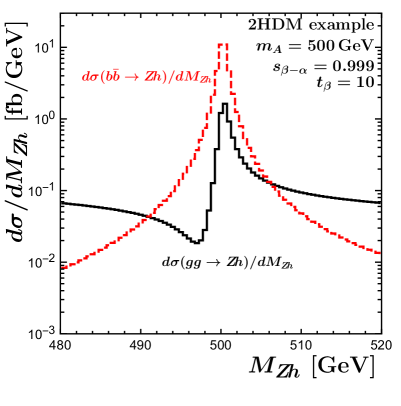
Figure 6: The cross sections $gg\to Z\!h{}$ (black) and $b\bar{b}\to Z\!h{}$ (red) as a function of the invariant mass of the $Z\!h{}$ system for the LHC at $13$ TeV. The shapes are determined by the interference of the resonant $gg/b\bar{b}\to A\to Z\!h{}$ contributions with all other diagrams.

5.2 Minimal Supersymmetric Standard Model

Concerning the quark-loop contributions to the $gg\to Z\phi{}$ process, the MSSM amplitudes are identical to those of a type-II 2HDM. As explained in Ref.[17], the squark-loop contributions to CP-even Higgs production vanish, and of the squark-loop contributions to CP-odd Higgs production, only triangle-type diagrams are non-vanishing. We compared the results for the quark- and the squark-loop diagrams for both CP-even and -odd Higgs production from Ref.[17] to our own calculation of the $gg\to Z\phi{}$ cross section based on FormCalc [16] and found agreement after fixing some typos in Ref.[17].

Similar to the 2HDM, the parameters for the MSSM mode VHATNNLO(1)=1 can be defined in several ways. The first one is through the blocks 2HDM, MASS, and SQUARK. The block SQUARK is only required for CP-odd Higgs production, i.e. for VHATNNLO(2)=21. As described in detail in Table 14, its entries define the masses and mixing of stops and sbottoms. For the squark mixing angle $\theta_{q}$ ($q\in\{t,b\}$) both conventions $\cos\theta_{q}\in[-1,1]$ and $\sin\theta_{q}\in[0,1]$ or vice versa are possible. If $\sin\theta_{q}$ is not specified, the convention with $\cos\theta_{q}\in[-1,1]$ is assumed, and $\sin\theta_{q}\geq 0$ is obtained from $\sqrt{1-\cos^{2}\theta_{q}}$. Since we work at leading order for what concerns squark effects, the renormalization scheme of these parameters is arbitrary. Furthermore, vh@nnlo does not restrict the range of values for $A_{t}$, $A_{b}$ and $\mu$. However, we urge the user to choose these parameters in accordance to the squark masses and mixings, which limits their ranges. The Feynman rules for the squark couplings can be found in Ref.[55]. They involve also the quark masses $m_{b}$ and $m_{t}$, for which we insert the $\overline{\mbox{{MS}}}$ value $m_{b}(m_{b})$ provided in SMPARAMS(5), and the on-shell value $m_{t}$ of SMPARAMS(6), respectively.

Another way to provide the MSSM parameters is through the link of vh@nnlo to the code FeynHiggs [64, 65, 66, 67, 68, 69, 70] (see Appendix B.3 on how to establish this link). If the input file contains the Block FEYNHIGGS, vh@nnlo will ignore the blocks 2HDM, MASS, and SQUARK, but rather call the program FeynHiggs to determine the spectrum and the couplings of the specific MSSM parameter point. A number of flags for FeynHiggs can be accessed through the block FEYNHIGGSFLAGS. A detailed description of the two blocks is given in Table 15 and 16. The blocks associated with the link to FeynHiggs generally understand all input parameters as on-shell. Accordingly, stop and sbottom masses returned from FeynHiggs are renormalized on-shell. In case the link to FeynHiggs is active, vh@nnlo also allows to incorporate the resummation of $\tan\beta$-enhanced sbottom contributions in the bottom-quark Yukawa coupling, known as $\Delta_{b}$ resummation [71, 72, 73, 74, 75, 76]. Setting ORDER(10)=1 will activate the so-called “full resummation” as presented in Eqs. (16c)–(16e) of Ref.[55]. Note that one may also define an independent value of $\Delta_{b}$ by adjusting the bottom-quark Yukawa coupling through Block FACTORS, see Table 8.

A third option to provide the relevant MSSM input is through an additional SLHA-style input file, referred to as “spectrum file” in what follows, which contains the MSSM particle spectrum. The relevant content and a list of potential spectrum generators providing a spectrum file are given in Appendix B.3. This mode of operating vh@nnlo is activated by including a Block SPECTRUMFILE in the actual input file of vh@nnlo, and specifying the path to the spectrum file in SPECTRUMFILE(1). Apart from that, the vh@nnlo input file only requires the generic blocks described in Sect. 3, as well as the widths of the Higgs bosons in entries 250,350 and 360 in Block MASS.

Block SQUARK
entry	meaning
1	mass of $\tilde{t}_{1}$, $\tilde{m}_{t1}$ [GeV]
2	mass of $\tilde{t}_{2}$, $\tilde{m}_{t2}$ [GeV]
3	stop mixing angle $\cos\theta_{t}$
4	stop mixing angle $\sin\theta_{t}$
5	trilinear coupling $A_{t}$ [GeV]
11	mass of $\tilde{b}_{1}$, $\tilde{m}_{b1}$ [GeV]
12	mass of $\tilde{b}_{2}$, $\tilde{m}_{b2}$ [GeV]
13	sbottom mixing angle $\cos\theta_{b}$
14	sbottom mixing angle $\sin\theta_{b}$
15	trilinear coupling $A_{b}$ [GeV]
20	gluino mass $|M_{3}|$ [GeV]
21	$\mu_{\rm{SUSY}{}}$ [GeV]

Table 14: Input parameters of Block SQUARK. For details, see main text.

Block FEYNHIGGS
entry	default	meaning
0		$\tan\beta$
1		soft-breaking mass $M_{1}$ [GeV]
2		soft-breaking mass $M_{2}$ [GeV]
3		soft-breaking mass $M_{3}$ [GeV]
10		generic trilinear coupling $A_{x}$ [GeV]
11-19	$A_{x}$	trilinear couplings $A_{t},A_{b},A_{\tau},A_{c},A_{s},A_{\mu},A_{u},A_{d},A_{e}$ [GeV]
23		$\mu_{\rm{SUSY}{}}$ [GeV]
26		pseudoscalar Higgs mass $m_{A}$ [GeV]
30		generic soft-breaking mass $M_{\rm{SUSY}{}}$ [GeV]
31-36	$M_{\rm{SUSY}{}}$	soft-breaking masses M1SL,M2SL,M3SL,M1SE,M2SE,M3SE [GeV]
41-49	$M_{\rm{SUSY}{}}$	soft-breaking masses M1SQ,M2SQ,M3SQ,M1SU,M2SU,M3SU,
		M1SD,M2SD,M3SD [GeV]

Table 15: Input parameters of Block FEYNHIGGS. The entries FEYNHIGGS(11-19) and FEYNHIGGS(31-49) are automatically set to the generic values FEYNHIGGS(10) and FEYNHIGGS(30), if they are not specified. The notation of the soft-breaking masses follows the notation of FeynHiggs.

Block FEYNHIGGSFLAGS
entry	default	meaning
1	4	mssmpart
2	0	fieldren
3	0	tanbren
4	2	higgsmix
5	4	p2approx
6	2	looplevel
7	1	runningMT
8	1	botResum
9	0	tlCplxApprox
10	3	loglevel

Table 16: Input parameters of Block FEYNHIGGSFLAGS as they are compatible with FeynHiggs 2.13.0 and 2.14.0. For the meaning and ranges (dependent on the FeynHiggs version) of the settings we refer to the FeynHiggs webpage [77]. If they are not specified they are automatically set to the default values of FeynHiggs 2.13.0. The settings fieldren and tanbren were removed in FeynHiggs 2.14.0.

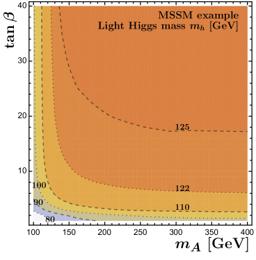
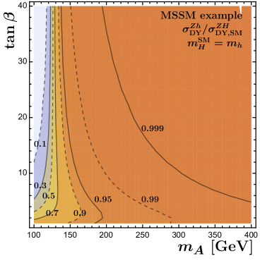
(a)	(b)
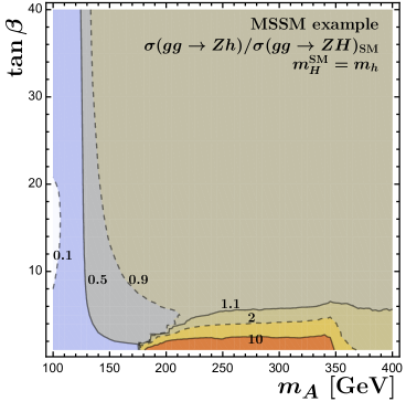
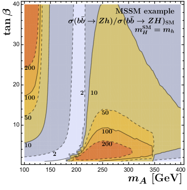
(c)	(d)

Figure 7: Normalized production of a light Higgs boson in the MSSM as a function of $m_{A}$ in GeV and $\tan\beta$ showing (a) the Higgs mass in GeV; (b) the DY-like cross section; (c) the gluon-induced cross section and (d) the bottom-quark initiated cross section. All cross sections are normalized to the SM Higgs cross section obtained for the same Higgs mass.

We present a numerical example for light Higgs production in association with a $Z$ boson in the MSSM in Fig. 7 for the $13$ TeV LHC. The Higgs mass and mixing is obtained from FeynHiggs 2.13.0 for an MSSM scenario with relatively heavy SUSY masses, $M_{\text{SUSY}}=2$ TeV, $m_{Q3}=m_{U3}=m_{D3}=1.5$ TeV, $M_{1}=M_{2}=1$ TeV, $M_{3}=2.5$ TeV, $\mu=1$ TeV and $A_{t}=A_{b}=A_{\tau}=(2.7+1.5/\tan\beta)$ TeV. Since there are no squark contributions to $Z\!h{}$ production at order $\mathcal{O}(\alpha_{s}^{2})$, the features correspond to the well-known decoupling behavior for the light Higgs boson. Since all SUSY states are above $1$ TeV, they do not enter the pseudoscalar total decay width, which is relevant for the sub-processes $gg\to Z\!h{}$ and $b\bar{b}\to Z\!h{}$.

Fig. 7 (a) shows the light Higgs mass in the $m_{A}$-$\tan\beta$-plane as obtained by FeynHiggs. Only for large enough values of $m_{A}$ and $\tan\beta$, a light Higgs mass $m_{h}$ in the range of $(125\pm 3)$ GeV is reached through higher-order corrections to the light Higgs boson mass, which at tree-level is bound to be below the $Z$-boson mass $m_{Z}$. This is the decoupling region, i.e. all light Higgs boson couplings to SM particles are close to their SM value. This explains the behavior of the DY-like component to Higgs Strahlung, shown in Fig. 7 (b), since it directly follows the squared coupling $(g_{VV}^{h})^{2}$ of the light Higgs boson $h$ to gauge bosons $V\in\{W,Z\}$. All components of the cross sections in Fig. 7 (b)–(d) are normalized to their corresponding SM results, assuming $m_{H}^{\text{{SM}}}=m_{h}$ for each parameter point.

The gluon-fusion induced component $gg\to Z\!h{}$, depicted in Fig. 7 (c), reveals a richer structure. For low values of $m_{A}\lesssim 150$ GeV, it is $g_{VV}^{h}\ll 1$, so that the contribution from triangle diagrams is small, whereas the box diagrams proportional to the Higgs Yukawa couplings depend on $\tan\beta$. In fact, the minimal cross section is obtained for intermediate values of $\tan\beta$, where the coupling $g_{t}^{h}$ to top quarks is reduced w.r.t. the SM, and the coupling $g_{b}^{h}$ to bottom quarks is not significantly enhanced. Towards larger values of $m_{A}$, decoupling is reached rather quickly. However, for $m_{A}\gtrsim m_{h}+m_{Z}$, the contribution $gg\to A\to Z\!h{}$ can be kinematically resonant. It plays an important role for low values of $\tan\beta$, where it enhances the cross section relative to the SM Higgs cross section by more than a factor of $10$. The fact that this effect extends to values of $m_{A}$ below $200$ GeV is due to the reduced light Higgs boson mass $m_{h}<100$ GeV at low values of $\tan\beta$. For larger values of $\tan\beta$, the coupling $g_{VV}^{h}$ quickly approaches $1$, while the coupling $g_{Z}^{Ah}$ almost vanishes. Thus the contribution $gg\to A\to Z\!h{}$ is only relevant for very low values of $\tan\beta$, where at the same time the Yukawa coupling of the pseudoscalar $g_{t}^{A}$ is large. Another kinematic threshold is observed at $m_{A}\approx 2m_{t}$, where the decay $A\to t\bar{t}$ opens up. The increased pseudoscalar width $\Gamma_{A}$ reduces the contribution due to $gg\to A\to Z\!h{}$.

Finally, we present the component $b\bar{b}\to Z\!h{}$ in Fig. 7 (d). The MSSM cross section exceeds the SM cross section (which is tiny) by one to two orders of magnitude almost throughout the entire $m_{A}$-$\tan\beta$-plane. For $m_{A}\lesssim 150$ GeV, i.e. outside the decoupling region, the light-Higgs-boson bottom-quark Yukawa coupling $g_{b}^{h}$ is strongly dependent on $\tan\beta$, which explains the steep increase of the cross section with $\tan\beta$. Relevant Feynman diagrams are the $t$- and $u$-channel contributions shown in Fig. 2 (a) and (b). For $m_{A}\gtrsim 200$ GeV, those Feynman diagrams are less relevant, since the light-Higgs-boson bottom-quark Yukawa coupling $g_{b}^{h}$ approaches its SM value—though slightly slower than the top-quark Yukawa coupling $g_{t}^{h}$. On the other hand, the pseudoscalar contribution $b\bar{b}\to A\to Z\!h{}$ is manifest (see Fig. 2 (c)), since the pseudoscalar can be resonant. Here the strong enhancement of the pseudoscalar bottom-quark Yukawa coupling $g_{b}^{A}$ with increasing $\tan\beta$ leads to observable differences also at high values of $\tan\beta$ despite the fact that $g_{Z}^{Ah}$ almost vanishes, i.e. decoupling is reached. We note that for this example we did not include $\Delta_{b}$ resummation.

SUSY scenario	$m_{Q3}=m_{U3}=m_{D3}$	$X_{t}$ [GeV]	$(m_{\tilde{t}_{1}},m_{\tilde{t}_{2}})$	$(m_{\tilde{b}_{1}},m_{\tilde{b}_{2}})$
	[GeV]	$A_{b}=A_{t}$	[GeV,GeV]	[GeV,GeV]
1	$3000$	$3500$	$(2902,3103)$	$(2999,3003)$
2	$3000$	$0$	$(3004,3004)$	$(2998,3004)$
3	$1200$	$2300$	$(1035,1365)$	$(1196,1210)$
4	$1200$	$0$	$(1211,1211)$	$(1194,1212)$
5	$600$	$1000$	$(464,748)$	$(589,622)$
6	$600$	$0$	$(622,623)$	$(586,624)$

Table 17: Choice of squark masses for the $p_{T}{}$ and $M_{Z\!\phi{}}$ distributions shown in Fig. 8.

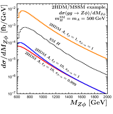
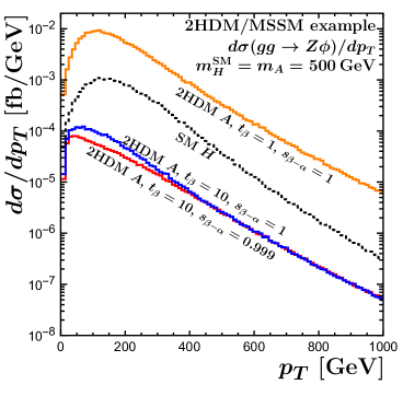
(a)	(b)
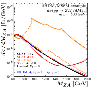
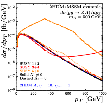
(c)	(d)

Figure 8: Invariant mass $M_{Z\!\phi{}}$ and $p_{T}{}$ distributions for a pseudoscalar $A$ with mass $m_{A}=500$ GeV produced in $gg\to Z\!A{}$ at the $13$ TeV LHC: (a) and (b) compare the distributions of a SM Higgs (with $m_{H}=500$ GeV) and different 2HDM scenarios; (c) and (d) compare the pure 2HDM case with $\tan\beta=10$ and decoupling $\sin(\beta-\alpha)=1$ with additional squark contributions. The SUSY scenarios are defined in Table 17.

Before we close our discussion on the MSSM, we show $p_{T}{}$ distributions and $M_{Z\!\phi{}}$ distributions for the gluon-induced production of a pseudoscalar with a mass of $500$ GeV to demonstrate the influence of squark contributions. The cross sections are produced for the $13$ TeV LHC. We choose $\tan\beta=10$ and $\mu=1$ TeV and pick six choices of squark masses shown in Table 17. Again we link to FeynHiggs version 2.13.0 to obtain the light Higgs mass as well as the squark masses. Only scenarios $1$ and $3$ yield a light Higgs mass in accordance with experimental data, i.e. within $125\pm 3$ GeV. Scenario $6$ yields the lowest mass with $110$ GeV. Such scenarios can be considered pedagogical examples to demonstrate squark mass thresholds and the influence of $X_{t}$. The process $gg\to Z\!A{}$ also has a light and heavy Higgs contribution $gg\to\{h,H\}\to Z\!A{}$, where the former vanishes for exact decoupling $g_{VV}^{h}=1$, i.e. $g_{Z}^{Ah}=0$. The squark contributions in exact decoupling are thus relevant only for $gg\to H\to Z\!A{}$. In Fig. 8 (a) and (b) we first show the influence of the choice of $\tan\beta$ in a 2HDM of type II and compare it with the distribution of a “SM Higgs” with the same mass of $500$ GeV. Also the influence of $gg\to\{h,H\}\to Z\!A{}$ can be inferred from the difference between $\sin(\beta-\alpha)=1$ and $\sin(\beta-\alpha)=0.999$. The choice of $\tan\beta=10$ minimizes the cross section, since again $g_{t}^{A}$ is reduced, while $g_{b}^{A}$ is only moderate. Therefore one expects large relative squark effects in this region of the parameter space, which we show in Fig. 8 (c) and (d). Indeed, in the invariant mass distribution, the squark mass thresholds are clearly visible in scenarios 5+6. Given that the partonic center-of-mass energy $\sqrt{\hat{s}}$ has to fulfill $\hat{s}\geq m_{\phi}^{2}+m_{Z}^{2}+2p_{T}^{2}+2\sqrt{(m_{Z}^{2}+p_{T}^{2})(m_{\phi}^{2}+p_{T}^{2})}$, also the $p_{T}{}$ distribution in scenario 5 probes the squark mass thresholds $2m_{\tilde{t}_{1}}$ and $2m_{\tilde{t}_{2}}$ at around $p_{T}{}\approx 320-330$ GeV and $p_{T}{}\approx 660-670$ GeV, respectively. Also the inclusive cross section in scenario 5 is enhanced by a factor of more than $20$, due to resonant squark contributions. It is remarkable that even larger squark masses still lead to a significant deformation at low $p_{T}{}$ and $M_{Z\!\phi{}}$ of the distributions, in particular in case of large squark mixing $X_{t}\neq 0$. However, the cross sections are very small and hard to access experimentally.

5.3 CP mixing among Higgs bosons

By default, vh@nnlo assumes the Higgs CP eigenstates $(h,H,A)$ of the 2HDM and the MSSM to be identical to the mass eigenstates $(h_{1},h_{2},h_{3})$. However, it does provide the option for a naive mixing according to

$$\begin{split}\left(\begin{array}[]{c}h_{1}\\ h_{2}\\ h_{3}\end{array}\right)=R\left(\begin{array}[]{c}h\\ H\\ A\end{array}\right)\,,\end{split}$$ (5)

where the orthogonal rotation matrix $R$ is parametrized in the form

$$\begin{split}\qquad R=\begin{pmatrix}c_{12}c_{13}&s_{12}c_{13}&s_{13}\\ -s_{12}c_{23}-c_{12}s_{23}s_{13}&c_{12}c_{23}-s_{12}s_{23}s_{13}&s_{23}c_{13}\\ s_{12}s_{23}-c_{12}c_{23}s_{13}&-c_{12}s_{23}-s_{12}c_{23}s_{13}&c_{23}c_{13}\end{pmatrix}\end{split}$$ (6)

with $c_{ij}=\cos\theta_{ij}$ and $s_{ij}=\sin\theta_{ij}$. The three independent angles $\theta_{12}$, $\theta_{13}$, and $\theta_{23}$ can be specified in the input file. For all but the $gg\to Z\phi$ and the $b\bar{b}\to Z\phi$ contributions, this simply results in a modification of the $VV\phi$ couplings according to

$$\begin{split}g^{i}_{VV}=\sum_{\phi\in\{h,H,A\}}R_{i\phi}\,g^{\phi}_{VV}\,,\end{split}$$ (7)

where $R_{ih},R_{iH},R_{iA}$ refer to the first, second, and third column of the matrix $R$, respectively, the $g^{\phi}_{VV}$ ($V\in\{W,Z\}$) are the couplings of the specified model without CP mixing (see Eq. (2) and Fig. 5), and $g^{i}_{VV}$ is the coupling constant for the $h_{i}VV$ vertex. Note that, up to the sign, $\theta_{12}$ has the same meaning as $\alpha$, defined in Eq. (2) for the 2HDM, since both angles determine the rotation among the two CP-even Higgs eigenstates. We keep this redundancy in vh@nnlo for the sake of a transparent implementation of the mixing.

Finally, we note that the rotation defined through Block HCPMIX is applied after a possible rescaling of the couplings by the entries in Block FACTORS (see Table 8 in Sect. 3).

Block HCPMIX
entry	default	meaning
1	$0.$	$\theta_{12}$
2	$0.$	$\theta_{13}$
3	$0.$	$\theta_{23}$

Table 18: The mixing angles for CP mixing in radian.

The $gg\to Z\phi$ component of the partonic cross section for a specific $\phi$ involves also the other two Higgs bosons through $s$-channel exchange. vh@nnlo combines the corresponding helicity amplitudes by assuming a CP-even and a CP-odd coupling of each Higgs mass eigenstate to the top and the bottom quarks, according to

$$\begin{split}{\cal L}_{\text{Y}}=-\sum_{j=1}^{3}\sum_{q\in\{b,t\}}\frac{m_{q}}{v}\bar{q}\left[\sum_{\phi\in\{h,H\}}R_{j\phi}g_{q}^{\phi}-iR_{jA}g_{q}^{A}\gamma_{5}\right]qh_{j}\end{split}$$ (8)

and using the appropriate $h_{i}h_{j}Z$ couplings

$$\begin{split}g^{ij}_{Z}=\sum_{\phi\in\{h,H\}}\left(R_{iA}R_{j\phi}-R_{i\phi}R_{jA}\right)g^{A\phi}_{Z}\,,\end{split}$$ (9)

where $g^{\phi}_{q}$ and $g^{A\phi}_{Z}$ are again the $q\bar{q}\phi$ and $ZA\phi$ coupling constants of the specified model without CP mixing (see Table 11, Eq. (3), and Fig. 5). Currently, the $b\bar{b}\to Z\phi$ component cannot be evaluated with CP mixing within vh@nnlo, so ORDER(4) needs to be set to -1 when CP mixing is switched on. Mixing is activated by including the Block HCPMIX in the input file, where the mixing angles are specified, see Table 18. In order to obtain the cross section for $h_{1}$, $h_{2}$, or $h_{3}$ production, one needs to set VHATNNLO(2) to 11, 12, or 21, respectively. Similarly, the masses $m_{h_{1}}$, $m_{h_{2}}$, and $m_{h_{3}}$ are defined through MASS(25,35,36), respectively.

Instead of a consistent implementation of CP violation in the MSSM through complex parameters, vh@nnlo simply assumes that the quark and vector-boson couplings of the Higgs are modified as described above, and in addition, the Higgs-squark couplings are affected by an analogous rotation:

$$\begin{split}g^{q,i}_{kl}=\sum_{\phi\in\{h,H,A\}}R_{i\phi}g^{q,\phi}_{kl}\,,\qquad k,l\in\{1,2\}\,,\end{split}$$ (10)

where $g^{q,\phi}_{kl}$ is the coupling constant of $\phi$ to the squarks $\tilde{q}_{k}$ and $\tilde{q}_{l}$ in the CP-conserving MSSM, see Ref.[55]. This approach misses contributions due to CP violation in the squark sector, which induces new couplings of the three neutral eigenstates $\{h,H,A\}$ to squarks.

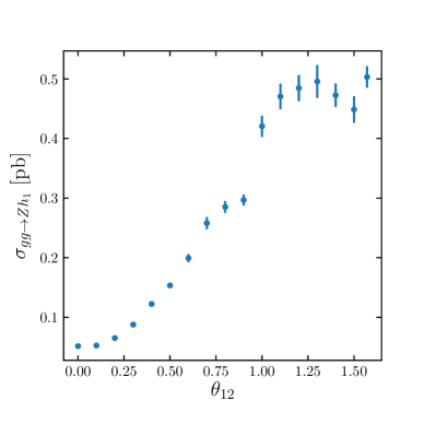
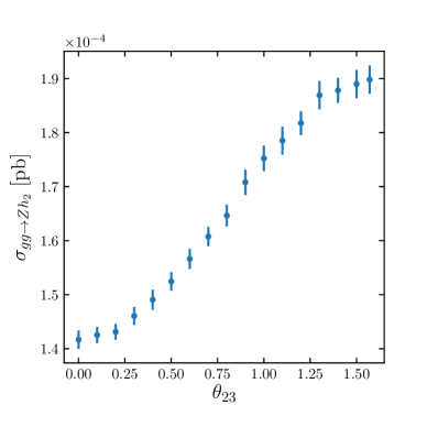
(a)	(b)
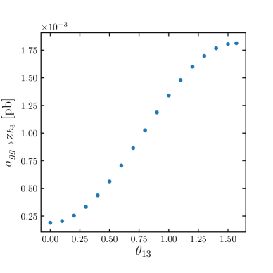
(c)

Figure 9: The $gg\to Z\phi$ component of $Z\!h$ production including CP mixing for the production of $h_{1}$, $h_{2}$, and $h_{3}$. The left end of each plot corresponds, from $(a)$–$(c)$, to the production of $h$, $H$, and $A$ within a type-II 2HDM with $\tan\beta=20$ and $\sin(\beta-\alpha)=1$. The Higgs masses are set to $m_{h_{1}}=125$ GeV and $m_{h_{2}}=m_{h_{3}}=300$ GeV.

As an example, Fig. 9 shows the dependence of the $gg\to Z\phi$ contribution to the cross section on one of the relevant mixing parameters successively for $\phi=\phi_{1}$, $\phi_{2}$, and $\phi_{3}$. No mixing corresponds to a type-II 2HDM with $\tan\beta=20$ and $\sin(\beta-\alpha)=1$ in this figure. The Higgs boson masses are $m_{h_{1}}=125$ GeV and $m_{h_{2}}=m_{h_{3}}=300$ GeV. As the mixing angle $\theta_{ij}$ increases, the produced Higgs boson $h_{i}$ gradually assumes the CP properties and the couplings of what is $h_{j}$ in the unmixed case, while the mass remains unchanged.

5.4 Vector-like quarks

Vector-like quarks (VLQs) impact the gluon-initiated contribution to Higgs Strahlung. We adopt the general parametrization of Ref.[37] for adding a single multiplet of vector-like quarks (VLQs) to the SM Lagrangian. There are seven possible representations which can mix with the SM quarks through Yukawa interactions [78, 79]. They all involve vector-like quarks $T$ and/or $B$ with electric charges $+2/3$ and $-1/3$, respectively, and possibly one of $X$ and $Y$, with electric charges $+5/3$ and $-4/3$. In this way, one arrives at two singlets, three doublets, and two triplets:

$$\text{singlets}: 1 :(T)\,, 2 :(B)\,,$$

$$\text{doublets}: 3 :(XT)\,, 4 :(TB)\,, 5 :(BY)\,,$$ (11)

$$\text{triplets}: 6 :(XTB)\,, 7 :(TBY)\,.$$

Sizable mixing is only assumed between $T$ and $t$, and $B$ and $b$, where $t$ and $b$ are the SM top and bottom quark. In each case, this mixing is parametrized by an angle $\theta^{q}$ and a phase $\phi^{q}$:

$$\begin{split}\left(\begin{matrix}q\\ Q\end{matrix}\right)=\left(\begin{matrix}\cos\theta^{q}&-e^{i\phi^{q}}\sin\theta^{q}\\ e^{-i\phi^{q}}\sin\theta^{q}&\cos\theta^{q}\end{matrix}\right)\left(\begin{matrix}q^{0}\\ Q^{0}\end{matrix}\right)\,,\end{split}$$ (12)

where the superscript “0” denotes the weak eigenstates in order to distinguish them from the mass eigenstates. This parametrization of the mixing applies to $(q,Q)=(b,B)$ and $(q,Q)=(t,T)$, and separately to their left- and right-handed components. The left- and right-handed mixing angles are related by

$$\tan\theta^{q}_{R}=\frac{m_{q}}{m_{Q}}\tan\theta_{L}^{q}$$ for singlets and triplets, and (13)

$$\tan\theta^{q}_{L}=\frac{m_{q}}{m_{Q}}\tan\theta_{R}^{q}$$ for doublets. (14)

The phases $\phi^{q}$ are the same for the left- and right-handed components. For the triplet representations, one finds an additional constraint of the form

$$\begin{split}\sin 2\theta_{L}^{b}=a\frac{m_{T}^{2}-m_{t}^{2}}{m_{B}^{2}-m_{b}^{2}}\sin 2\theta_{L}^{t}\,,\end{split}$$ (15)

where $a=\sqrt{2}$ for the triplet $(X,T,B)$, and $a=1/\sqrt{2}$ for the triplet $(T,B,Y)$. Since the $T$ and $B$ quark share the same mass term in the Lagrangian, there is another constraint on the mass splitting of the form

$$m_{T}^{2}\cos^{2}\theta_{R}^{t}+m_{t}^{2}\sin^{2}\theta_{R}^{t} =m_{B}^{2}\cos^{2}\theta_{R}^{b}+m_{b}^{2}\sin^{2}\theta_{R}^{b} \text{for $(TB)$},$$ (16a)

$$m_{T}^{2}\cos^{2}\theta_{L}^{t}+m_{t}^{2}\sin^{2}\theta_{L}^{t} =m_{B}^{2}\cos^{2}\theta_{L}^{b}+m_{b}^{2}\sin^{2}\theta_{L}^{b} \text{for triplets}.$$ (16b)

Without mixing, the VLQs as introduced here would not couple to the Higgs boson, and their couplings to the $Z$ boson would be purely vector like. This means that they would not contribute to the $gg\to Z\!H$ process at LO due to charge conjugation invariance (Furry’s theorem). In fact, the LO amplitude for $gg\to Z\!H$ does not involve $X$ and $Y$ for this reason.

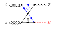
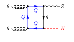
(a)	(b)	(c)
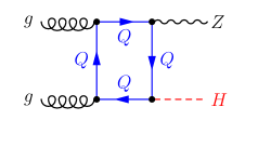
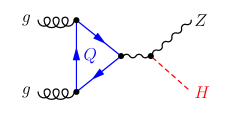
(d)	(e)

Figure 10: New contributions to the $gg\to Z\!H$ amplitude due to VLQs. Here, $Q\in\{B,T\}$, and $q$ is the SM quark which mixes with $Q$.

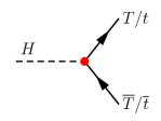
	$\displaystyle=-i\frac{em_{T/t}Y_{TT/tt}}{2M_{W}s_{W}}$
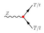
	$\displaystyle=i\frac{e}{2c_{W}s_{W}}\gamma^{\mu}\left(2Q_{t}s_{W}^{2}-\frac{X^{L}_{TT/tt}+X^{R}_{TT/tt}}{2}+\frac{X^{L}_{TT/tt}-X^{R}_{TT/tt}}{2}\gamma_{5}\right)$
	$\displaystyle=-i\frac{em_{T}}{2M_{W}}\left(\frac{Y^{L}_{tT}+Y^{R}_{tT}}{2}+\frac{Y^{R}_{tT}-Y^{L}_{tT}}{2}\gamma_{5}\right)$
	$\displaystyle=-i\frac{e}{2c_{W}s_{W}}\gamma^{\mu}\left(\frac{X^{L}_{tT}+X^{R}_{tT}}{2}+\frac{X^{R}_{tT}-X^{L}_{tT}}{2}\gamma_{5}\right)$

Figure 11: Feynman rules for the Higgs and $Z$ couplings due to a vector-like $T$ quark calculated with FeynRules [80, 81].

However, aside from modified $t\bar{t}Z$, $b\bar{b}Z$, $t\bar{t}H$, and $b\bar{b}H$ coupling constants with respect to their SM values, the mixing in the top and bottom sector leads to $t\bar{T}Z$, $b\bar{B}Z$, $t\bar{T}H$, and $b\bar{B}H$ vertices, an axial-vector component of the $T\bar{T}Z$ and $B\bar{B}Z$ coupling, and non-vanishing $B\bar{B}H$ and $T\bar{T}H$ couplings. The LO effects of the VLQs on the $gg\to Z\!H$ process are therefore as follows: (i) a modification of the SM box contributions; (ii) additional box contributions involving one to four $T$ or $B$ propagators, see Fig. 10 (a)–(d); (iii) additional triangle contributions involving $T$ or $B$, see Fig. 10 (e). The Feynman rules corresponding to the vertices of two $T$ quarks with a Higgs or $Z$, and a single $T$ quark with a top quark, a Higgs or a $Z$ boson are listed in Fig. 11 with generic couplings. Here, $Q_{t}$ is the electric charge of the $t$ (and the $T$) quark, $X^{L/R}_{TT}$ and $X^{L/R}_{tt}$ are the left- and right-handed couplings of the $T$ and $t$ quark to the $Z$ boson, respectively; $Y_{TT}$ and $Y_{tt}$ are the Yukawa couplings of the $T$ and $t$ quark; and $X^{L/R}_{tT}$ and $Y^{L/R}_{tT}$ are the left- and right-handed couplings of a $T$ and $t$ quark to a $Z$ boson and a Higgs. Note that vertices for a vector-like $B$ quark can be obtained by introducing an additional minus sign to the couplings and changing $T\to B$, $t\to b$. The generic couplings assume values which are specific to the various representations. A full list can be found in Ref.[37]. The couplings of VLQs to gluons are the same as for SM quarks. The amplitudes including VLQs have been evaluated with the help of FormCalc.

The input block for VLQs in vh@nnlo is described in Table 19. VLQ(1) fixes the representation for the VLQs according to Eq. (11); vh@nnlo sets the generic couplings discussed above according to this representation; VLQ(2) and VLQ(3) set the mass of the $T$ and $B$ quark, respectively; the left- and right-handed mixing angles for the bottom sector are set in VLQ(4) and VLQ(5), respectively, and in VLQ(7) and VLQ(8) for the top sector; finally, the phases for the bottom and top mixing can be set in VLQ(6) and VLQ(9). Note that there are conditions like Eq. (15) which constrain these parameters; the input will be checked for consistency by vh@nnlo. In fact, most conveniently the user may provide only an independent subset of the parameters, and let vh@nnlo determine the remaining parameters from the theoretical constraints described above. Specifically, for the $(TB)$ doublet, it is sufficient to provide one of the following sets:

1. $m_{B}$, $m_{T}$, and one mixing angle;

2. $m_{B}$, ($\theta_{L}^{b}$ or $\theta_{R}^{b}$) and $\theta_{R}^{t}$;

3. $m_{T}$, ($\theta_{L}^{t}$ or $\theta_{R}^{t}$) and $\theta_{R}^{b}$.

For the triplets $(TBY)$ and $(XTB)$, possible input sets are:

1. $m_{B}$ and ($\theta_{L}^{b}$ or $\theta_{R}^{b}$);

2. $m_{T}$ and ($\theta_{L}^{t}$ or $\theta_{R}^{t}$).

Note, however, that the left- or right-handed mixing angle will always be calculated for any representation, if only one of these mixings and the corresponding mass of the vector-like quark is set as input. The complete set of parameters, including the coupling factors appearing in Fig. 11, are listed in Block VLQ in the output file.

Block VLQ
entry	range	meaning
1	{1,$\ldots$,7}	VLQ representation
2		$m_{B}$ [GeV]
3		$m_{T}$ [GeV]
4		$\theta_{L}^{b}$
5		$\theta_{R}^{b}$
6		$\phi^{b}$
7		$\theta_{L}^{t}$
8		$\theta_{R}^{t}$
9		$\phi^{t}$

Table 19: Setting the parameters for vector-like quarks. The number of the representation refers to Eq. (11).

To study the impact of VLQs on the total cross section, we define the ratios $R_{\theta}$ and $R_{\phi}$,

$$R_{\theta}=\frac{\sigma_{gg\to Z\!H{},\text{{SM}{}}+\text{{VLQ}{}s}}}{\sigma_{gg\to Z\!H,\text{{SM}{}}}}\Bigg{|}_{\phi^{t/b}=0},\quad R_{\phi}=\frac{\sigma_{gg\to Z\!H{},\text{{SM}{}}+\text{{VLQ}{}s}}}{\sigma_{gg\to Z\!H,\text{{SM}{}}+\text{{VLQ}{}s}}|_{\phi^{t/b}=0}}\Bigg{|}_{\theta_{L/R}^{t/b}\neq 0}.$$ (17)

In $R_{\theta}$ we normalize the total cross section of $gg\to Z\!H{}$ with VLQs at a given value of $\theta_{L/R}^{t/b}$ to the total cross section of the gluon induced contribution of the SM. Moreover, we restrict ourselves to cases with $\phi^{t/b}=0$. For $R_{\phi}$ we choose $\theta_{L/R}^{t/b}\neq 0$ since otherwise the VLQ will have no effect on the cross section. Thus, instead of normalizing this result to the SM alone, we add the contributions of the VLQs for $\phi^{t/b}=0$ in the denominator. Additionally, for $R_{\phi}$ we set $\phi^{t}=\phi^{b}$. We choose the masses and the dominant mixing angle of the vector-like $T$ partner as our input scheme for singlets and doublets, and $m_{T}$ with $\theta_{L}^{t}$ as the input for the triplets.

Fig. 12 shows these ratios for four different representations of VLQs by varying $\theta_{L}^{t}$ (for singlets and triplets) or $\theta_{R}^{t}$ for doublets in (a) and $\phi^{t/b}$ in (b). The other settings are described in the caption of the figure. We first discuss Fig. 12 (a) in detail: All curves start at the SM cross section for zero mixing angle, where the VLQs have no couplings to the SM particles. For the vector-like top singlet (T), the total cross section for $gg\to Z\!H{}$ steadily increases with the mixing angle, until it reaches a maximum of about $1.5$ times the SM cross section at maximal mixing, i.e. $\theta_{L}^{t}=\tfrac{\pi}{2}$, where the couplings of the $t$ and the $T$ are exactly interchanged w.r.t. the SM. Therefore, the cross section at $\theta_{L}^{t}=\tfrac{\pi}{2}$ is the SM value for a hypothetical top quark mass of $600$ GeV.

This is also true for the $(XT)$ doublet, where the contributing diagrams are the same as for the $(T)$ singlet. Since the couplings are different, however, and the dominant mixing is the right-handed one, the intermediate evolution of the cross section differs from the $(T)$ singlet. It reaches almost $\sim 200\%$ of the SM cross section at about $\theta_{R}^{t}=1.1$, which is mainly due to the enhancement of the coupling to $t$ in this region (as can be seen in Fig. 13).

For the $(TB)$ doublet, the behavior is strikingly different. While it resembles the behavior of a $(T)$ singlet at low mixing angles, which is due to the dominance of the top quark in this regime, it quickly drops down to very small values as the mixing increases towards $\tfrac{\pi}{4}$, before it nearly vanishes at maximal mixing, where $T$ and $B$ assume the couplings of their SM partners, while those of $t$ and $b$ vanish. Although both VLQs carry the same mass, at maximal mixing their couplings to the SM bosons slightly differ due to Eq. (14). If they coupled equally, their amplitudes would be of equal magnitude but of opposite sign for maximal mixing, such that they would completely cancel in the cross section. The same behavior would be observed in the SM, if the $b$ and the $t$ quark had identical masses.

Finally, the contributing diagrams for the $(TBY)$ triplet are the same as for the $(TB)$ doublet, but with different couplings. We therefore do not see the same cancellation as for the ($TB$) doublet, which is even more suppressed since only at minimal and maximal mixing the $T$ and $B$ masses are degenerate. Instead, one observes similar features as in $(XT)$, with the maximum shifted towards $\theta_{R}^{t}=1.1$. At maximal mixing, the cross section again assumes the value found for $(T)$ and $(XT)$. In this case, however, all SM and $T$ quark contributions vanish, and the $B$ quark is the only contribution left. Since for maximal mixing one finds $m_{B}=m_{T}=600$ GeV and the couplings are the same as for the $(T)$ singlet, their results coincide.

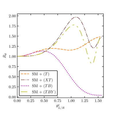
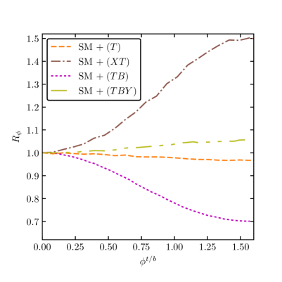
(a)	(b)

Figure 12: Total gluon induced cross section for $Z\!H{}$ production with additional VLQ multiplets normalized to the gluon induced production in the SM for different mixing angles $\theta_{L/R}^{t}$ (a) and different phases $\phi^{t}=\phi^{b}$ (b). The vector-like quark masses are set to $m_{T}=m_{B}=600$ GeV. In the case of the triplet $(TBY)$, only $m_{T}=600$ GeV is assumed and the mixing angle $\theta_{L}^{b}$ together with the mass $m_{B}$ are calculated accordingly to Eq. (15) and Eq. (16b).

In Fig. 12 (b) we can observe the impact of $\phi^{t/b}$ for the four different representations. The mixing angle of the top and bottom sector is set to $\theta_{L}^{t/b}=\tfrac{\pi}{16}$, where in the case of the triplet $\theta_{L}^{b}$ and $m_{B}$ are calculated according to Eq. (15) and Eq. (16b). Since the phase $\phi^{t/b}$ only appears in mixed couplings of quarks, vector-like-quarks and SM bosons, one can probe the magnitude of the contributions in which these mixed vertices appear. For the case of $gg\to Z\!H{}$ this only affects box diagrams. Here, we set $\phi^{t}=\phi^{b}$ for doublets and triplets which contain both $T$ and $B$ quarks. The shape is determined by the dependence on $\exp(i\phi^{t/b})$ in the couplings, and varying the phase can lead to an enhancement of up to $50\%$ for the $(XT)$ doublet and a reduction of $-30\%$ for the $(TB)$ doublet. For the studied $(T)$ singlet and the $(TBY)$ triplet the effect of the phases is rather mild.

Kinematic distributions are typically much more sensitive to effects of new physics than the total cross section. Thus we study the $p_{T}$ and $M_{Z\!H{}}$ distributions with an additional multiplet. Again we emphasize that $p_{T}$ refers to the transverse momentum of the Higgs boson. For the $(T)$, $(XT)$ and $(TB)$ multiplets, we fix $m_{T}=m_{B}=600$ GeV, set the mixing angle such that we are in a maximum of Fig. 12, and calculate the remaining input parameters with vh@nnlo. For the $(TBY)$ triplet, we only fix $m_{T}=600$ GeV and $\theta_{L}^{t}=1.06$. Moreover, for all multiplets we set $\phi^{t/b}=0$. In Fig. 13 we show (a) the $p_{T}$ and (b) the $M_{Z\!H}$ distributions of the gluon initiated process in comparison to the SM expectation. In the $p_{T}$ spectra we see an overall enhancement of the SM distribution which is more distinct in the boosted regime, i.e. $p_{T}\gtrsim 200$ GeV. The threshold of the top quark at $p_{T}\sim 150$ GeV and the threshold of the VLQs at about $p_{T}\sim 590$ GeV is visible for all representations and more pronounced for $(T)$ and $(XT)$ than the other studied cases.

The invariant mass is more sensitive to threshold effects than the transverse momentum, thus showing distinct peaks at $M_{Z\!H{}}\approx 2m_{t}$ and at twice the VLQ masses. It shares the same features as the $p_{T}$ distributions, i.e. the VLQ contributions lead to an overall enhancement in comparison to the SM, which is more distinct in the boosted regime. Since the VLQ masses are not degenerate for the scenario of the $(TBY)$ triplet studied here, we observe in total three thresholds, one for the top quark, one for the $B$ quark at about $900$ GeV, and one for the $T$ quark at about $1.2$ TeV.

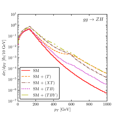
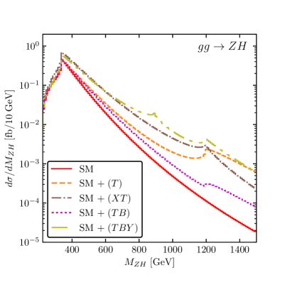
(a)	(b)

Figure 13: Transverse momentum (a) and invariant mass (b) distributions in the SM for the gluon induced process compared to the SM with an additional VLQ multiplet The input parameters are $m_{T}=m_{B}=600$ GeV for all representations other than $(TBY)$, where $m_{T}=600$ GeV is chosen and $m_{B}=447.08$ GeV. The mixing angles are $\theta_{L}^{t}=0.5$ for $(T)$, $\theta_{R}^{t}=1.02$ for $(XT)$, $\theta_{R}^{t}=0.471$ for $(TB)$, and $\theta_{L}^{t}=1.06$ for $(TBY)$.

5.5 Higher-dimensional operators

Finally, we describe the implementation of higher-dimensional operators, which is independent of a concrete model implementation. In the SM, our setup allows to set bounds on the implemented higher-dimensional operators. On the other hand, our implementation can also be used in the MSSM or the 2HDM for the production of a CP-even Higgs boson and a $Z$ boson, where additionally one dimension-5 operator coupling two gluons to a pseudoscalar can be taken into account. In our choice of the dimension-6 operators, we adopt the so-called gauge basis of Refs.[82, 83] with their corresponding FeynRules implementation [84], but restrict ourselves to the operators which involve third-generation quarks. We allow these operators to be added to any implemented model, i.e. the SM, the 2HDM and the MSSM, but note that we only implemented operators relevant for the production of the light SM-like CP-even Higgs boson $gg\to Z\!h{}$. The effective Lagrangian reads

$${\cal L}={\cal L}_{\rm{SM}/{2HDM}/{MSSM}}+\sum_{i=1}^{6}{\cal L}_{i}\,,$$ (18)

where the sum is over the following higher-dimensional operators:

$$\begin{split}{\cal L}_{1}&=i\frac{c_{HQ}}{v^{2}}\left[\bar{Q}_{L}\gamma^{\mu}Q_{L}\right]\left[\Phi^{\dagger}\overleftrightarrow{D}_{\mu}\Phi\right]\,,\\ {\cal L}_{2}&=i\frac{c_{Ht}}{v^{2}}\left[\bar{t}_{R}\gamma^{\mu}t_{R}\right]\left[\Phi^{\dagger}\overleftrightarrow{D}_{\mu}\Phi\right]\,,\\ {\cal L}_{3}&=i\frac{4c^{\prime}_{HQ}}{v^{2}}\left[\bar{Q}_{L}\gamma^{\mu}T_{2k}Q_{L}\right]\left[\Phi^{\dagger}T_{2k}\overleftrightarrow{D}_{\mu}\Phi\right]\,,\\ {\cal L}_{4}&=\frac{4g_{s}c_{tG}}{M_{W}^{2}}Y^{\text{{SM}}}_{t}\Phi^{\dagger}\bar{Q}_{L}\gamma^{\mu\nu}T_{a}t_{R}G_{\mu\nu}^{a}+\text{h.c.}\,,\\ {\cal L}_{5}&=-\frac{c_{t}}{v^{2}}Y_{t}\Phi^{\dagger}\Phi\Phi^{\dagger}\bar{Q}_{L}t_{R}+\text{h.c.}\,,\\ {\cal L}_{6}&=\frac{g_{s}^{2}c_{A}}{32\pi^{2}v}G^{a,\mu\nu}\tilde{G}^{a}_{\mu\nu}A\,.\end{split}$$ (19)

Herein, we define the dual gluon field-strength tensor $\tilde{G}^{a}_{\mu\nu}=\frac{1}{2}\epsilon_{\mu\nu\alpha\beta}G^{a,\alpha\beta}$ ($\epsilon_{0123}=+1$), $\gamma^{\mu\nu}=\frac{i}{4}[\gamma^{\mu},\gamma^{\nu}]$, and $T_{2k}=\sigma_{k}/2$, with the Pauli matrices $\sigma_{k}$. The Hermitian derivative operator $\overleftrightarrow{D}_{\mu}$ is given by $\Phi^{\dagger}\overleftrightarrow{D}_{\mu}\Phi=\Phi^{\dagger}D_{\mu}\Phi-(D_{\mu}\Phi^{\dagger})\Phi$.

Eq. (19) is set up as an extension of the SM Lagrangian, which means that, in the SM mode of vh@nnlo, $\Phi$ is the SM Higgs doublet. However, vh@nnlo also allows to use Eq. (19) for CP-even Higgs production in BSM models, in which case the same Feynman rules for Eq. (19) as those derived in the SM are assumed, with the Higgs particle being interpreted as the one specified in VHATNNLO(2). Note in particular that $Y^{\text{{SM}}}_{t}$ in Eq. (19) is always replaced by $\sqrt{2}m_{t}/v$, while $Y_{t}$ is set to the Yukawa coupling of the model specified in VHATNNLO(2). All other couplings of the Higgs are taken into account according to the model under consideration.

Except for ${\cal L}_{4}$, which differs by the sign, our notation follows Ref.[84]. Fig. 14 depicts selected Feynman diagrams arising from the inclusion of higher dimensional operators. The operator ${\cal L}_{6}$ is a dimension-5 operator which can have a significant impact in extended Higgs sectors and is therefore added to the Lagrangian. In the 2HDM or the MSSM, it corresponds to an effective coupling among two gluons and the pseudoscalar $A$ at LO, relevant for the contribution $gg\to A\to Z\!h{}$. This involves the $g_{Z}^{Ah}$ coupling, see Eq. (3), as well as finite width effects for the pseudoscalar $A$, see the discussion in Sect. 5.1.

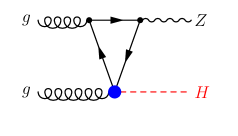
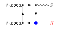
(a)	(b)	(c)
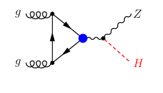
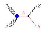
(d)	(e)

Figure 14: Sample Feynman diagrams for contributions to $gg\to Z\!H{}$ through dimension-6 operators. The Feynman diagrams (a), (c) and (d) can alternatively have modified $gq\bar{q}$ (through ${\cal L}_{4}$) or $Zq\bar{q}$ couplings (through ${\cal L}_{1,2,3}$). (e) shows the contribution of the dimension-5 operator ${\cal L}_{6}$ for $gg\to Z\!h{}$ in a 2HDM/the MSSM.

The coefficients of the operators in ${\cal L}_{i}$ are specified through entries $i$ in Block DIM in the vh@nnlo input file. We list them in Table 20. We note that by default all coefficients are understood to be constants. However, by specifying an input scale through DIM(11), the running of $c_{tG}$ to the renormalization scale following Ref.[85] is included. The strong coupling constant $g_{s}=\sqrt{4\pi\alpha_{s}}$ is evaluated at the renormalization scale $\mu_{\text{R}}$. In contrast to other input blocks which parametrize new physics, vh@nnlo inserts the default values given in Table 20; i.e. any unspecified coefficient of Eq. (19) is set to zero. The range of values for the coefficients is unrestricted in principle, but it is clear that very large values are potentially non-perturbative, and thus the results of vh@nnlo will be unreliable.

Block DIM
entry	default	range	meaning
1	$0.$	see text	$c_{HQ}$
2	$0.$	see text	$c_{Ht}$
3	$0.$	see text	$c^{\prime}_{HQ}$
4	$0.$	see text	$c_{tG}$
5	$0.$	see text	$c_{t}$
6	$0.$	see text	$c_{A}$
10	$0$	{0,1}	add terms of order $\mathcal{O}(c_{i}^{2}+c_{i}c_{j})$: {no, yes}
11	-1.	-1.,>0.	scale of $c_{tG}$ [GeV] (no running: -1.)

Table 20: Coefficients of dimension-6 operators are specified in Block DIM.

The effect of the dimension-6 operators is two-fold in general: on the one hand, they lead to additional vertices which do not occur in the model under consideration; on the other hand, they may modify the coupling constants of the existing vertices. vh@nnlo takes both of these effects into account. Some of these operators have been already implemented in Ref.[36] with a different normalization. To compare our results to Tab. 7 of Ref.[36] one has to transform the effective couplings as follows:

$$c_{HQ} \to c_{\phi Q}^{(1)}\frac{2m_{t}^{2}}{\Lambda^{2}}\,,\qquad c_{Ht}\to c_{\phi t}\frac{2m_{t}^{2}}{\Lambda^{2}}\,,$$ (20)

$$c^{\prime}_{HQ} \to c_{\phi Q}^{(3)}\frac{2m_{t}^{2}}{\Lambda^{2}}\,,\qquad c_{tG}\to c_{tG}\frac{M_{W}^{2}}{2\Lambda^{2}}\,,$$

where $\Lambda$ is the energy scale of new physics. On the right-hand side of Eq. (20), the couplings are normalized and named as in Ref.[36]. For $\Lambda=1$ TeV, $m_{t}=173.3$ GeV, $M_{W}=79.824$ GeV and $c_{\phi Q}^{(1)}=c_{\phi t}=c_{\phi Q}^{(3)}=c_{tG}=1$ we obtain

$$c_{HQ}=c_{Ht}=c^{\prime}_{HQ}=0.0600658\quad\mathrm{and}\quad c_{tG}=0.00318594\,.$$ (21)

The total cross section can now be written as

$$\sigma=\sigma_{\text{{SM}{}}}+\sigma^{(1)}+\sigma^{(2)}\,,$$ (22)

where $\sigma_{\text{{SM}{}}}$ is the total cross section of the Standard Model, $\sigma^{(1)}$ contains the interference of the SM amplitudes which involves one modified vertex, and $\sigma^{(2)}$ contains the interference of amplitudes of different operators, where at most one modified vertex is inserted, or the square of an amplitude with one modified vertex. Again, the amplitudes have been calculated with the help of FormCalc.

In Table 21 we show the results for the total cross section of gluon initiated $Z\!h$ production at $\sqrt{s}=8$ and $13$ TeV by taking into account $\mathcal{L}_{1,2,4,5}$, with the couplings of Eq. (21), and $c_{t}=0.1$. The effect of $\mathcal{L}_{3}$ is not shown since it leads to the same results as $\mathcal{L}_{2}$. We only enable one dimension-6 operator at a time. Furthermore, we fix the scales to $\mu_{\text{R}}=\mu_{\text{F}}=125$ GeV, use the LO MSTW2008 [86] parton distribution functions, and set $m_{b}=0$. We observe full agreement with Ref.[36] within the numerical accuracy. As is well-known, the largest effects of such operators typically occur at high transverse momenta or high invariant masses, where the validity of the effective field theory description becomes questionable. In the case of $Z\!h$ production, however, the operators under consideration only affect the $gg\to Z\!H$ component of the cross section, which is known to affect mostly the kinematic region at and slightly above the top quark threshold. In order to investigate the impact of the dimension-6 operators in more detail, we employ the ratio of the full cross section to its DY-like component $R_{\text{\text{{DY}}}}^{Z\!H}\equiv\sigma^{Z\!H}/\sigma^{Z\!H}_{\text{\text{{DY}}}}$, from which one obtains

$$\begin{split}\sigma_{gg\to Z\!H}/\sigma_{\text{\text{{DY}}}}^{Z\!H}=R_{\text{\text{{DY}}}}^{Z\!H}-1\,.\end{split}$$ (23)

This quantity was shown in Ref.[87] to be particularly suited for a data-driven extraction of the gluon-initiated component $\sigma_{gg\to Z\!H}$ from experiment. Using the example of $\mathcal{L}_{1}$ and $\mathcal{L}_{4}$, Fig. 15 shows that large effects of the dimension-6 operators can already be observed in the few-hundred-GeV region of both $p_{T}$ and $M_{Z\!H}$, i.e., well in the validity range of the effective theory. This observation adds to the virtues of the $Z\!H$ process in the search of New Physics.

$\sqrt{s}/\text{TeV}$	$\sigma_{\text{{SM}{}}}/\text{fb}$		$\mathcal{L}_{1}$	$\mathcal{L}_{2}$	$\mathcal{L}_{4}$	$\mathcal{L}_{5}$
8	29.19	$\sigma^{(1)}/\text{fb}$	$1.71$	$-1.72$	$10.37$	$-4.31$
		$\sigma^{(2)}/\text{fb}$	$0.0471$	$0.0473$	$1.604$	$0.292$
		$\sigma^{(1)}/\sigma_{\text{{SM}{}}}$	$0.059$	$-0.059$	$0.355$	$-0.147$
		$\sigma^{(2)}/\sigma^{(1)}$	$0.028$	$-0.028$	$0.155$	$-0.068$
13	94.12	$\sigma^{(1)}/\text{fb}$	$5.87$	$-5.92$	$34.47$	$-14.98$
		$\sigma^{(2)}/\text{fb}$	$0.176$	$0.185$	$6.18$	$1.17$
		$\sigma^{(1)}/\sigma_{\text{{SM}{}}}$	$0.062$	$-0.063$	$0.366$	$-0.159$
		$\sigma^{(2)}/\sigma^{(1)}$	$0.029$	$-0.031$	$0.179$	$-0.078$

Table 21: Cross sections for $gg\to Z\!H{}$ production at the LHC at $\sqrt{s}=8$ TeV and $\sqrt{s}=13$ TeV for the SM and the dimension-6 operators in analogy to Ref.[36].

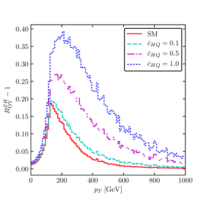
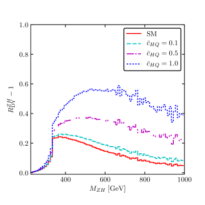
(a)	(b)
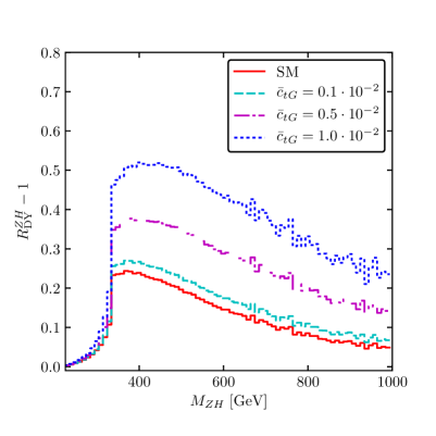
(c)	(d)

Figure 15: Example of the impact of different dimension-6 operators on kinematic distributions while only including the interference term of the new operators and the SM.

6 Conclusions

We presented version 2 of the code vh@nnlo, which allows to study various new-physics aspects in Higgs Strahlung. In detail we described the general structure of the code and its control through an input file containing SLHA-inspired blocks. We implemented the Higgs sectors of a 2HDM, which—in type II—also allows for the calculation of MSSM cross sections for Higgs Strahlung. For this purpose, we added the relevant squark amplitudes to the gluon-initiated contribution of Higgs Strahlung. In addition, the bottom-quark initiated contribution is given at leading-order in perturbation theory and resonances of (pseudo)scalars are included in both gluon- and bottom-quark initiated contributions. We demonstrated their relevance for light Higgs production in the MSSM. The shape of their interferences with the non-resonant Feynman diagrams can be studied, but a thorough analysis is left for future work. CP mixing among the three 2HDM scalars can be taken into account. Vector-like quarks can be studied in the SM, which—depending on the representation and the mixing angles—can have a significant effect on the inclusive cross section and the kinematical distributions. vh@nnlo can also provide the transverse momentum distribution of the final state Higgs boson, and invariant mass distributions of the two-particle final state. For the DY-like component, this requires a link to MCFM. We showed threshold effects of vector-like quarks and squarks in both distributions. Lastly, beyond such concrete model implementations, vh@nnlo now includes higher-dimensional operators. We compared our implementation to the literature and found agreement. It turns out that their effect is particularly pronounced directly above the top-quark threshold, which is well below the cut-off which is typically assumed for the underlying effective field theory. Apart from the already mentioned internal link to MCFM, the new version of vh@nnlo can also be linked to FeynHiggs and 2HDMC for the calculation of Higgs masses and mixings. Other dependencies on external codes are described throughout the manuscript.

Appendix A Installation and execution of vh@nnlo

vh@nnlo can be downloaded from Ref.[1]. After unpacking it, the user has to run ./configure, which determines local Fortran and C++ compilers and library dependencies. Thereafter, the user should open the Makefile of vh@nnlo and adjust the paths to the various needed external codes, see Appendix B.1. Then make will result in an executable, which is placed in the newly generated /bin folder. This executable is run by typing
./x.vhnnlo input.in output.out,
where input.in has to be an input file, which contains the various blocks described throughout the manuscript. Example input files for the various new-physics models and for distributions can be found in the folder /example. If the name of the output file output.out is not specified, it is named out.vh. In case vh@nnlo is recompiled we recommend to type make recompile to make sure that a few dependencies are newly set up. If this does not result in the desired behavior, a previous make (some)clean can be helpful. If vh@nnlo should be linked to 2HDMC or FeynHiggs, the Makefile has to be processed with an additional predef=2HDMC or FH. If vh@nnlo was compiled beforehand, it has to be accompanied by recompile, i.e. make recompile predef=2HDMC or FH. Note that adding GGZH=NO allows to compile without the gluon-induced component. In that case, also the link to LoopTools is not required.

Appendix B Links to external codes

First, vh@nnlo has to be linked to LHAPDF for the usage of modern PDF sets, the CUBA package for numerical integration, LoopTools for the calculation of loop integrals and potentially MCFM for the calculation of kinematic distributions. As we described in Sect. 5.1 and Sect. 5.2 vh@nnlo can be linked to external codes for the calculation of Higgs boson masses and decay widths. Those are 2HDMC for the 2HDM and FeynHiggs for the MSSM. We subsequently describe the various needed and potential links to external codes.

B.1 LHAPDF, CUBA and LoopTools

vh@nnlo needs to be linked to LHAPDF [53], which allows to make use of up-to-date PDF sets. We recommend to use LHAPDF version 6.2 or higher. Also older versions $\geq$ 6 work, but might produce an unpleasant flow of LHAPDF screen messages. After downloading [88] and installing LHAPDF into a local directory, the user has to specify the paths to the LHAPDF installation folder in the vh@nnlo Makefile variables LHAPDFDIR, LHAPDFINCDIR and LHAPDFLIBDIR, where the latter two folders have to include relevant header files and contain the LHAPDF library, respectively. If LHAPDF is installed in a global directory like /usr/share, etc., the specification of the paths might be obsolete. Note that the PDF sets, which were specified in the input file of vh@nnlo, need to be installed, i.e. downloaded from the LHAPDF webpage [88]. This can for example be done through the LHAPDF script lhapdf install.

Block VEGAS
entry	default	meaning
10	10000	DY starting points
11	5000	DY increase points
12	20000	DY minimal points
13	1000000	DY maximal points
20	10000	$gg$ starting points
21	0	$gg$ increase points
22	10000	$gg$ minimal points
23	70000	$gg$ maximal points
30	10000	$b\bar{b}$ starting points
31	5000	$b\bar{b}$ increase points
32	200000	$b\bar{b}$ minimal points
33	500000	$b\bar{b}$ maximal points

Table 22: Integration parameters.

For numerical integration vh@nnlo makes use of the CUBA package [89] which needs to be installed separately. The paths to the CUBA installation directory is then specified in the variable CUBADIR in the Makefile of vh@nnlo. For the numerical integration, vh@nnlo uses CUBA’s implementation of VEGAS algorithm. The central integration parameters can be controlled through Block VEGAS in the input file of vh@nnlo, see Table 22. These are the number of evaluations the numerical integration is starting with, the increase in the number of evaluations, and the minimal and maximal number of evaluations. They are specified in VEGAS(10+10$\cdot i$), VEGAS(11+10$\cdot i$), VEGAS(12+10$\cdot i$) and VEGAS(13+10$\cdot i$), respectively, where $i\in\{0,1,2\}$ labels the DY-like component, the gluon- and the bottom-quark initiated contribution, respectively.

Finally, for the evaluation of loop integrals, vh@nnlo requires a link to LoopTools [91, 16], which can be obtained from Ref.[92]. We recommend to use LoopTools version 2.13 or higher. The link to the LoopTools installation directory and the library is specified in the variables LTDIR and LTLIBDIR of the vh@nnlo Makefile, respectively. If vh@nnlo is compiled with GGHZ=NO, i.e. the gluon-induced component is not included, the link to LoopTools is not needed.

B.2 MCFM

MCFM can be downloaded from its webpage [93]. It has to be compiled and installed separately. Since the implementation of vh@nnlo is currently not compatible with OpenMP, the MCFM library should be built and linked without OpenMP, if a link to vh@nnlo should be established. vh@nnlo can be linked to MCFM 8 by adjusting the path specified in the variable MCFMDIR and setting the corresponding flag MCFM=YES in the Makefile of vh@nnlo. Since MCFM needs some additional files in the working directory, one has to call make MCFM to copy them into the vh@nnlo directory. The interface to MCFM does not rely on input files, thus all parameters needed by MCFM are set internally, except the input given in the input block DISTRIB. This includes the start, end and bin width of the histogram, cuts on the invariant mass of $M_{V\!H{}}$ and the integration points for VEGAS, see Table 10. All SM parameters, the factorization and renormalization scale and the parton distribution function are set to the same values as given in the blocks SMPARAMS, SCALES and PDFSPEC, respectively. To produce results comparable to vh@nnlo we disable the decays of $H$, $Z$, and $W$. This disables automatically any jets so that all input regarding jets is filled with dummy variables. The remaining input values for MCFM, which are automatically set by vh@nnlo, are summarized in Table 23.

parameter	value	meaning
ewscheme	3	EW scheme
aemmz_inp	from vh@nnlo	$\alpha_{\mathrm{EM}}(M_{Z})$
xw_inp	from vh@nnlo	$s_{W}^{2}$
nproc	101 ($Z\!H{}$), 96 ($W^{-}H$), 91 ($W^{+}H$)	Process number
zerowidth	.true.	Remove decay width
removebr	.true.	Disable decay

Table 23: Input parameters for MCFM set in vh@nnlo automatically.

B.3 2HDMC, FeynHiggs and SLHA-style Higgs sector input

After downloading the code 2HDMC from the webpage [94] and installing it, the path to the 2HDMC installation needs to be supplied through the variable 2HDMCPATH in the Makefile of vh@nnlo. Compiling vh@nnlo with make predef=2HDMC establishes the link between vh@nnlo and 2HDMC. If vh@nnlo was already compiled before without the link, one should do make recompile predef=2HDMC. Note that only recent versions of 2HDMC allow to include the $H_{2}$ basis.

FeynHiggs can be obtained from its webpage [77]. After installation, vh@nnlo can be linked to FeynHiggs by specifying the full path in FHPATH in the Makefile of vh@nnlo. In addition, since different versions of FeynHiggs differ in their input and/or output format, vh@nnlo requires the version number of FeynHiggs in the variable FHVERSION. vh@nnlo has been tested with FeynHiggs 2.9 through 2.14, which is the latest publicly available version.

Another option is to use vh@nnlo through an additional SLHA-style spectrum file. Its name is provided in the vh@nnlo input file through SPECTRUMFILE(1). The additional SLHA-style spectrum file needs to contain the following blocks:

• Block MASS, for the on-shell masses of the gluino, $h$, $H$, $A$ boson, stop and sbottom quarks,

• Block AU and Block AD, for the soft-breaking trilinear stop-Higgs and sbottom-Higgs coupling, respectively,

• Block STOPMIX and Block SBOTMIX to evaluate the stop and sbottom mixing angle,

• Block ALPHA, for the scalar mixing angle $\alpha$,

• Block HMIX to get the values of the $\mu$ parameter and $\tan\beta$.

Note that these blocks are part of the standard output of typical SUSY spectrum generators such as SoftSusy [95], SPheno [96, 97], or FlexibleSUSY [98, 99, 100]. Combining the latter with Himalaya [101] allows to run vh@nnlo in the MSSM by taking into account three-loop corrections to the light Higgs boson mass [102, 103]. For now, vh@nnlo does not read in the Higgs boson decay width from the spectrum file, since not all external codes provide such numbers. Thus, the user needs to fill the entries MASS(250/350/360) in the vh@nnlo input file with the Higgs boson decay widths of the light CP even, the heavy CP even Higgs boson and the pseudoscalar, respectively. We refer to the example vh@nnlo input file together with a FlexibleSUSY spectrum file in folder /example.

References

- [1] https://web.physik.rwth-aachen.de/~harlander/software/vh@nnlo/
- [2] G. Aad et al. [ATLAS Collaboration], Phys. Lett. B 716 (2012) 1 [arXiv:1207.7214].
- [3] S. Chatrchyan et al. [CMS Collaboration], Phys. Lett. B 716 (2012) 30 [arXiv:1207.7235].
- [4] G. Aad et al. [ATLAS and CMS Collaborations], Phys. Rev. Lett. 114 (2015) 191803 [arXiv:1503.07589].
- [5] G. Aad et al. [ATLAS and CMS Collaborations], JHEP 1608 (2016) 045 [arXiv:1606.02266].
- [6] M. Aaboud et al. [ATLAS Collaboration], JHEP 1712 (2017) 024 [arXiv:1708.03299].
- [7] A. M. Sirunyan et al. [CMS Collaboration], arXiv:1709.07497.
- [8] O. Brein, R.V. Harlander, and T.J.E. Zirke, Comput. Phys. Commun. 184 (2013) 998 [arXiv:1210.5347].
- [9] T. Han and S. Willenbrock, Phys. Lett. B 273 (1991) 167.
- [10] O. Brein, A. Djouadi, and R.V. Harlander, Phys. Lett. B 579 (2004) 149 [hep-ph/0307206].
- [11] M.L. Ciccolini, S. Dittmaier, and M. Krämer, Phys. Rev. D 68 (2003) 073003 [hep-ph/0306234].
- [12] R. Hamberg, W.L. van Neerven, and T. Matsuura, Nucl. Phys. B 359 (1991) 343 Erratum: [Nucl. Phys. B 644 (2002) 403].
- [13] S. Dawson, T. Han, W.K. Lai, A.K. Leibovich, and I. Lewis, Phys. Rev. D 86 (2012) 074007 [arXiv:1207.4207].
- [14] O. Brein, R.V. Harlander, M. Wiesemann, and T. Zirke, Eur. Phys. J. C 72 (2012) 1868 [arXiv:1111.0761].
- [15] T. Hahn, Comput. Phys. Commun. 140 (2001) 418 [hep-ph/0012260].
- [16] T. Hahn and M. Perez-Victoria, Comput. Phys. Commun. 118 (1999) 153 [hep-ph/9807565].
- [17] B.A. Kniehl and C.P. Palisoc, Phys. Rev. D 85 (2012) 075027 [arXiv:1112.1575].
- [18] L. Altenkamp, S. Dittmaier, R.V. Harlander, H. Rzehak, and T.J.E. Zirke, JHEP 1302 (2013) 078 [arXiv:1211.5015].
- [19] R.V. Harlander, A. Kulesza, V. Theeuwes, and T. Zirke, JHEP 1411 (2014) 082 [arXiv:1410.0217].
- [20] R.V. Harlander, S. Liebler, and T. Zirke, JHEP 1402 (2014) 023 [arXiv:1307.8122].
- [21] J.F. Gunion, H.E. Haber, G.L. Kane, and S. Dawson, Front. Phys. 80 (2000) 1.
- [22] A.G. Akeroyd, Phys. Lett. B 377 (1996) 95 [hep-ph/9603445].
- [23] A.G. Akeroyd, J. Phys. G 24 (1998) 1983 [hep-ph/9803324].
- [24] M. Aoki, S. Kanemura, K. Tsumura, and K. Yagyu, Phys. Rev. D 80 (2009) 015017 [arXiv:0902.4665].
- [25] G.C. Branco, P.M. Ferreira, L. Lavoura, M.N. Rebelo, M. Sher, and J.P. Silva, Phys. Rept. 516 (2012) 1 [arXiv:1106.0034].
- [26] N. Craig, and S. Thomas, JHEP 1211 (2012) 083 [arXiv:1207.4835].
- [27] A. Djouadi, Phys. Rept. 459 (2008) 1 [hep-ph/0503173].
- [28] B. Hespel, F. Maltoni, and E. Vryonidou, JHEP 1506 (2015) 065 [arXiv:1503.01656].
- [29] C. Kao, Phys. Rev. D 46 (1992) 4907.
- [30] J. Yin, W.G. Ma, R.Y. Zhang, and H.S. Hou, Phys. Rev. D 66 (2002) 095008.
- [31] C. Kao, G. Lovelace, and L.H. Orr, Phys. Lett. B 567 (2003) 259 [hep-ph/0305028].
- [32] C. Kao and S. Sachithanandam, Phys. Lett. B 620 (2005) 80 [hep-ph/0411331].
- [33] L.L. Yang, C.S. Li, J.J. Liu, and L.G. Jin, J. Phys. G 30 (2004) 1821 [hep-ph/0312179].
- [34] Q. Li, C.S. Li, J.J. Liu, L.G. Jin, and C.-P. Yuan, Phys. Rev. D 72 (2005) 034032 [hep-ph/0501070].
- [35] J. Alwall et al., JHEP 1407 (2014) 079 [arXiv:1405.0301].
- [36] O. Bessidskaia Bylund, F. Maltoni, I. Tsinikos, E. Vryonidou, and C. Zhang, JHEP 1605 (2016) 052 [arXiv:1601.08193].
- [37] J.A. Aguilar-Saavedra, R. Benbrik, S. Heinemeyer, and M. Pérez-Victoria, Phys. Rev. D 88 (2013) no.9, 094010 [arXiv:1306.0572].
- [38] G. Ferrera, M. Grazzini, and F. Tramontano, Phys. Rev. Lett. 107 (2011) 152003 [arXiv:1107.1164].
- [39] G. Ferrera, M. Grazzini, and F. Tramontano, Phys. Lett. B 740 (2015) 51 [arXiv:1407.4747].
- [40] J.M. Campbell, R.K. Ellis, and C. Williams, JHEP 1606 (2016) 179 [arXiv:1601.00658].
- [41] A. Denner, S. Dittmaier, S. Kallweit, and A. Mück, JHEP 1203 (2012) 075 [arXiv:1112.5142].
- [42] J. M. Butterworth, A. R. Davison, M. Rubin and G. P. Salam, Phys. Rev. Lett. 100 (2008) 242001 [arXiv:0802.2470].
- [43] C. Englert, M. McCullough, and M. Spannowsky, Phys. Rev. D 89 (2014) no.1, 013013 [arXiv:1310.4828].
- [44] J.M. Campbell, R.K. Ellis, and C. Williams, JHEP 1107 (2011) 018 [arXiv:1105.0020].
- [45] J.M. Campbell and R.K. Ellis, Phys. Rev. D 60 (1999) 113006 [hep-ph/9905386].
- [46] J.M. Campbell, R.K. Ellis, and W.T. Giele, Eur. Phys. J. C 75 (2015) no.6, 246 [arXiv:1503.06182].
- [47] R. Boughezal, J.M. Campbell, R.K. Ellis, C. Focke, W. Giele, X. Liu, F. Petriello, and C. Williams, Eur. Phys. J. C 77 (2017) no.1, 7 [arXiv:1605.08011].
- [48] B.A. Kniehl, Phys. Rev. D 42 (1990) 2253.
- [49] D.A. Dicus and C. Kao, Phys. Rev. D 38 (1988) 1008 Erratum: [Phys. Rev. D 42 (1990) 2412].
- [50] A. Hasselhuhn, T. Luthe and M. Steinhauser, JHEP 1701 (2017) 073 [arXiv:1611.05881].
- [51] P.Z. Skands et al., JHEP 0407 (2004) 036 [hep-ph/0311123].
- [52] B.C. Allanach et al., Comput. Phys. Commun. 180 (2009) 8 [arXiv:0801.0045].
- [53] A. Buckley, J. Ferrando, S. Lloyd, K. Nordström, B. Page, M. Rüfenacht, M. Schönherr, and G. Watt, Eur. Phys. J. C 75 (2015) 132 [arXiv:1412.7420].
- [54] P. M. Ferreira, S. Liebler and J. Wittbrodt, Phys. Rev. D 97 (2018) no.5, 055008 [arXiv:1711.00024].
- [55] R.V. Harlander, S. Liebler, and H. Mantler, Comput. Phys. Commun. 184 (2013) 1605 [arXiv:1212.3249].
- [56] R.V. Harlander, S. Liebler, and H. Mantler, Comput. Phys. Commun. 212 (2017) 239 [arXiv:1605.03190].
- [57] S. Jung, Y.W. Yoon, and J. Song, Phys. Rev. D 93 (2016) no.5, 055035 [arXiv:1510.03450].
- [58] N. Greiner, S. Liebler, and G. Weiglein, Eur. Phys. J. C 76 (2016) no.3, 118 [arXiv:1512.07232].
- [59] B. Hespel, D. Lopez-Val, and E. Vryonidou, JHEP 1409 (2014) 124 [arXiv:1407.0281].
- [60] D. Eriksson, J. Rathsman, and O. Stål, Comput. Phys. Commun. 181 (2010) 189 [arXiv:0902.0851].
- [61] D. Eriksson, J. Rathsman, and O. Stål, Comput. Phys. Commun. 181 (2010) 833.
- [62] H.E. Haber and O. Stål, Eur. Phys. J. C 75 (2015) no.10, 491 Erratum: [Eur. Phys. J. C 76 (2016) no.6, 312] [arXiv:1507.04281].
- [63] G. Brooijmans et al., arXiv:1803.10379.
- [64] S. Heinemeyer, W. Hollik and G. Weiglein, Comput. Phys. Commun. 124 (2000) 76 [hep-ph/9812320].
- [65] S. Heinemeyer, W. Hollik and G. Weiglein, Eur. Phys. J. C 9 (1999) 343 [hep-ph/9812472].
- [66] G. Degrassi, S. Heinemeyer, W. Hollik, P. Slavich and G. Weiglein, Eur. Phys. J. C 28 (2003) 133 [hep-ph/0212020].
- [67] M. Frank, T. Hahn, S. Heinemeyer, W. Hollik, H. Rzehak and G. Weiglein, JHEP 0702 (2007) 047 [hep-ph/0611326].
- [68] T. Hahn, S. Heinemeyer, W. Hollik, H. Rzehak and G. Weiglein, Phys. Rev. Lett. 112 (2014) no.14, 141801 [arXiv:1312.4937].
- [69] H. Bahl and W. Hollik, Eur. Phys. J. C 76 (2016) no.9, 499 [arXiv:1608.01880].
- [70] H. Bahl, S. Heinemeyer, W. Hollik and G. Weiglein, Eur. Phys. J. C 78 (2018) no.1, 57 [arXiv:1706.00346].
- [71] T. Banks, Nucl. Phys. B 303 (1988) 172.
- [72] L.J. Hall, R. Rattazzi, and U. Sarid, Phys. Rev. D 50 (1994) 7048 [hep-ph/9306309].
- [73] R. Hempfling, Phys. Rev. D 49 (1994) 6168.
- [74] M. Carena, M. Olechowski, S. Pokorski, and C.E.M. Wagner, Nucl. Phys. B 426 (1994) 269 [hep-ph/9402253].
- [75] M. Carena, D. Garcia, U. Nierste, and C.E.M. Wagner, Nucl. Phys. B 577 (2000) 88 [hep-ph/9912516].
- [76] M. Carena, D. Garcia, U. Nierste, and C.E.M. Wagner, Phys. Lett. B 499 (2001) 141 [hep-ph/0010003].
- [77] http://feynhiggs.de
- [78] F. del Aguila, M. Perez-Victoria, and J. Santiago, Phys. Lett. B 492 (2000) 98 [hep-ph/0007160].
- [79] F. del Aguila, M. Perez-Victoria, and J. Santiago, JHEP 0009 (2000) 011 [hep-ph/0007316].
- [80] N.D. Christensen and C. Duhr, Comput. Phys. Commun. 180 (2009) 1614 [arXiv:0806.4194].
- [81] A. Alloul, N.D. Christensen, C. Degrande, C. Duhr, and B. Fuks, Comput. Phys. Commun. 185 (2014) 2250 [arXiv:1310.1921].
- [82] R. Contino, M. Ghezzi, C. Grojean, M. Mühlleitner, and M. Spira, JHEP 1307 (2013) 035 [arXiv:1303.3876].
- [83] S. Dawson, S. Dittmaier, and M. Spira, Phys. Rev. D 58 (1998) 115012 [hep-ph/9805244].
- [84] A. Alloul, B. Fuks, and V. Sanz, JHEP 1404 (2014) 110 [arXiv:1310.5150].
- [85] C. Zhang, Phys. Rev. D 90 (2014) no.1, 014008 [arXiv:1404.1264].
- [86] A.D. Martin, W.J. Stirling, R.S. Thorne, and G. Watt, Eur. Phys. J. C 63 (2009) 189 [arXiv:0901.0002].
- [87] R.V. Harlander, J. Klappert, C. Pandini and A. Papaefstathiou, arXiv:1804.02299 [hep-ph].
- [88] https://lhapdf.hepforge.org/
- [89] T. Hahn, Comput. Phys. Commun. 168 (2005) 78 [hep-ph/0404043].
- [90] http://www.feynarts.de/cuba/
- [91] G.J. van Oldenborgh and J.A.M. Vermaseren, Z. Phys. C 46 (1990) 425.
- [92] http://www.feynarts.de/looptools/
- [93] https://mcfm.fnal.gov/
- [94] http://2hdmc.hepforge.org
- [95] B.C. Allanach, Comput. Phys. Commun. 143 (2002) 305 [hep-ph/0104145].
- [96] W. Porod, Comput. Phys. Commun. 153 (2003) 275 [hep-ph/0301101].
- [97] W. Porod and F. Staub, Comput. Phys. Commun. 183 (2012) 2458 [arXiv:1104.1573].
- [98] P. Athron, J.H. Park, D. Stöckinger, and A. Voigt, Comput. Phys. Commun. 190 (2015) 139 [arXiv:1406.2319].
- [99] P. Athron, J.H. Park, T. Steudtner, D. Stöckinger, and A. Voigt, JHEP 1701 (2017) 079 [arXiv:1609.00371].
- [100] P. Athron, M. Bach, D. Harries, T. Kwasnitza, J.H. Park, D. Stöckinger, A. Voigt, and J. Ziebell, arXiv:1710.03760.
- [101] R.V. Harlander, J. Klappert, and A. Voigt, Eur. Phys. J. C 77 (2017) no.12, 814 [arXiv:1708.05720].
- [102] R.V. Harlander, P. Kant, L. Mihaila, and M. Steinhauser, Phys. Rev. Lett. 100 (2008) 191602 [Phys. Rev. Lett. 101 (2008) 039901] [arXiv:0803.0672].
- [103] P. Kant, R.V. Harlander, L. Mihaila, and M. Steinhauser, JHEP 1008 (2010) 104 [arXiv:1005.5709].