Cosmic Curvature Tested Directly from Observations

Abstract

Cosmic spatial curvature is a fundamental geometric quantity of the Universe. We investigate a model independent, geometric approach to measure spatial curvature directly from observations, without any derivatives of data. This employs strong lensing time delays and supernova distance measurements to measure the curvature itself, rather than just testing consistency with flatness. We define two curvature estimators, with differing error propagation characteristics, that can crosscheck each other, and also show how they can be used to map the curvature in redshift slices, to test constancy of curvature as required by the Robertson-Walker metric. Simulating realizations of redshift distributions and distance measurements of lenses and sources, we estimate uncertainties on the curvature enabled by next generation measurements. The results indicate that the model independent methods, using only geometry without assuming forms for the energy density constituents, can determine the curvature at the $\sim 6\times 10^{-3}$ level.

I Introduction

Spatial curvature is one of the two fundamental quantities defining the Robertson-Walker (RW) metric of a homogeneous and isotropic spacetime. Unlike spacetime curvature, which depends on the second derivative of the scale factor $a(t)$ entering the metric, spatial curvature $k$ is a purely geometric quantity. The most popular theories of early universe inflation predict spatial flatness $k=0$, so any detection of nonzero spatial curvature (hereafter just called curvature) would have significant impact on our understanding of the early universe and cosmic evolution. Moreover, if measurements of $k$ from observations at different redshift (or in different directions) significantly disagreed with each other, then this could call into doubt the Robertson-Walker metric and cosmic homogeneity and isotropy.

Many consistency tests or“alarms” for spatial flatness have been proposed (e.g. Clarkson et al. (2008); Shafieloo and Clarkson (2010); Mortsell and Jonsson (2011); Sapone et al. (2014); Räsänen et al. (2015); L’Huillier and Shafieloo (2017)), but here we focus on methods that actually deliver estimates of the curvature parameter $k$ or $\Omega_{k}=-k/(a_{0}H_{0})^{2}$, where $a_{0}H_{0}$ is the present expansion rate (see, for example, Bernstein (2006); Knox (2006)). Furthermore, we aim to have the curvature derived directly from the observations, without any derivatives taken of noisy data. Finally, we want to proceed in as model independent manner as possible, without using any dynamics from the Friedmann equations. Recall that spatial curvature is a geometric quantity, and so we can in principle test it by purely kinematic means, without imposing any equations of motion. That is, we never need to know the expansion factor $a(t)$ or the Hubble parameter $H(a)$.

These three principles ensure that any signals found of nonzero flatness, and in particular its evolution, arise from fundamental origins and not simply a misestimate of the matter density or numerical inaccuracy of differentiation of noisy data, say. Rather they will be as pure tests as we can enable of spatial curvature and of homogeneity and isotropy. For some other approaches to determining curvature see Takada and Dore (2015); Leonard et al. (2016); Sakr and Blanchard (2017); Witzemann et al. (2017).

In Sec. II we review the relation of curvature to distance measurements and derive an expression for $\Omega_{k}$ directly in terms of observables. In addition we derive a redshift dependent curvature function, the K test, that must hold for the RW metric. We model distance uncertainties and carry out their error propagation to curvature in Sec. III. In Sec. IV we discuss observational constraints from various realizations of future survey data. We summarize and conclude in Sec. V.

II Curvature and Distances

Triangulating a surface to measure its topography has an exceedingly long history. The generalization to nonEuclidean spaces showed that angle deficits and area deficits had an intimate relation to curvature. However, a single triangle generally requires measurement of angles as well as distances to test curvature, and this is not necessarily practical for cosmological observations (except for the angle at the observer).

Weinberg Weinberg (1972) applied a volume measure formed from distances (distances only, no angles) between four points in Tolkien’s Middle Earth, where a flat surface would have zero volume in the three space. This demonstrates a test of flatness (of a 2D surface) and a measurement of curvature. (In fact, for the distances given Middle Earth is not flat but has positive curvature with a measurable radius of curvature.)

The same can be applied in cosmology, where distances between two points can be measured either directly, if one point is at the observer, or through gravitational lensing if the two points lie along the same light ray reaching the observer. Unfortunately, “cross” distances, i.e. those between two lines of sight, cannot be measured geometrically easily (though they can statistically), and so the Middle Earth analogy fails. However, the expansion of the universe brings additional information so that a single triangle, associated with lens and source redshifts such that the light reaches the observer, can in fact measure curvature.

By measuring the distance to a gravitationally lensed source, $r_{s}$, to the object doing the lensing, $r_{l}$, and the distance between the two along the null geodesic followed by the light ray, $r_{ls}$, the curvature can be measured. In particular,

$$r_{ls}=r_{s}\sqrt{1+\Omega_{k}r_{l}^{2}}-r_{l}\sqrt{1+\Omega_{k}r_{s}^{2}}\ ,$$ (1)

where all $r$ are conformal distances. This follows from the properties of null geodesics in Robertson-Walker spacetime and does not depend at all on the Friedmann equations.

The quantity $\Omega_{k}$ is what we seek to determine. Here

$$\Omega_{k}=\frac{-k}{a_{0}^{2}H_{0}^{2}}\ ,$$ (2)

where $H_{0}$ is the Hubble constant and $a_{0}$ is the present scale factor of the universe. Recall that one cannot define $k=\pm 1$ and $a_{0}=1$ simultaneously – one can only normalize one or the other.

The distances $r_{l}$ and $r_{s}$ relative to the observer can be measured through geometric probes such as Type Ia supernova distances or baryon acoustic oscillations (BAO). The distance $r_{ls}$ between lens and source can be found through strong gravitational lensing; here we focus on the use of time delays between multiple images from a variable source as it is closer to a geometric probe. One could also use measurements of the image separation, and hence Einstein radius, though this may be more sensitive to lens modeling and dynamical measurements of the lens velocity dispersion.

The time delay distance is here defined as

$$D_{\Delta t}=\frac{r_{l}r_{s}}{r_{ls}}\ ,$$ (3)

where we omit the conventional prefactor of $1+z_{l}$ since that can itself be directly and accurately measured.

Putting together Eqs. (1) and (3) we can solve for the curvature in terms of observables,

$$\Omega_{k} = \frac{D_{\Delta t}^{2}}{4}\left(\frac{1}{r_{l}^{2}}-\frac{1}{r_{s}^{2}}-\frac{1}{D_{\Delta t}^{2}}\right)^{2}-\frac{1}{r_{s}^{2}}$$ (4)

$$= \frac{1}{4}\,\left[\frac{1}{D_{\Delta t}^{2}}-2\left(\frac{1}{r_{l}^{2}}+\frac{1}{r_{s}^{2}}\right)+D_{\Delta t}^{2}\left(\frac{1}{r_{l}^{2}}-\frac{1}{r_{s}^{2}}\right)^{2}\right]$$

This will be the central equation in our analysis.

Note that we have written all distances in terms of the dimensionless quantities $r_{i}$. For supernova and BAO distances, this is not unreasonable as they are measured relative to low and high redshift anchors respectively. Time delay distances however are dimensional quantities. If desired we can instead write all distance as dimensionful, i.e. $d_{i}=H_{0}^{-1}r_{i}$, and then the left hand side quantity of Eq. (4) we determine is really $\Omega_{k}H_{0}^{2}$, or more familiarly $\Omega_{k}h^{2}$ where $h$ is the reduced Hubble constant.

Motivated by a first order expansion of Eq. (1) for small curvature (cf. Bernstein (2006)) we could also establish a “K test”. This appears as

$$K(z_{l},z_{s}) \equiv \frac{1}{D_{\Delta t}}-\frac{1}{r_{l}}+\frac{1}{r_{s}}$$

$$\approx -\frac{1}{2}\Omega_{k}(r_{s}-r_{l})+{\mathcal{O}}(\Omega_{k}^{2})\ .$$

We emphasize that in this article we use the full form of the first line to test curvature, not just the first order expansion. The K test is useful to check: 1) Is this combination of distances consistent with $\Omega_{k}=0$?, and 2) If not, is its redshift dependence consistent with the Robertson-Walker prediction of Eq. (II)? We will investigate the use of both the full expression for $\Omega_{k}$ and the K test.

III Estimating Curvature

To carry out the curvature estimation we need a measurement of $D_{\Delta t}$ from a strongly lensed time delay system, and reconstructed distances at the redshifts $z_{l}$ and $z_{s}$, such as from a suite of supernova or BAO distances covering these redshifts. It would be more effective if the exact $r_{l}$ and $r_{s}$ could be measured directly but one is unlikely to have distances at exactly the right redshifts, and so must use an error-controlled interpolation procedure from data (using standardized candles – Type Ia supernovae – or rulers – BAO) at neighboring redshifts. Fortunately there have been already several successful statistical approaches proposed to reconstruct the distance-redshift relation (or indeed expansion history of the universe) in a model independent manner, which can be used to estimate cosmic distances at any given intermediate redshift without assuming a cosmological model, e.g. Shafieloo et al. (2006); Shafieloo (2007); Holsclaw et al. (2010, 2011); Shafieloo (2012); Shafieloo et al. (2012). Furthermore, such distances in future surveys will be much more densely measured in redshift than current data, simplifying the process.

One could possibly use a different combination of distances from the same strong lens system to get $r_{l}$, say, e.g. from the image angular separation or Einstein radius, but this would introduce lens modeling uncertainties. (Double source plane lenses Collett et al. (2012); Collett and Auger (2014); Linder (2016) offer another method to get geometric distances, but only as ratios of ratios.) We feel that systematic uncertainties from interpolation procedures are better understood than from the necessary lens modeling and dynamics. However, see Paraficz and Hjorth (2009); Jee et al. (2015, 2016). For a phenomenological, non-kinematic use of time delay distances in testing curvature see Liao et al. (2017); Li et al. (2018).

The uncertainty on the determination of the curvature is given in terms of the measurement uncertainties on the observables by

$$\sigma_{\Omega_{k}}^{2} = \frac{1}{4}\left[\left(\frac{1}{r_{l}^{2}}-\frac{1}{r_{s}^{2}}\right)^{2}D_{\Delta t}^{2}-\frac{1}{D_{\Delta t}^{2}}\right]^{2}\left(\frac{\sigma_{D_{\Delta t}}}{D_{\Delta t}}\right)^{2}$$ (6)

$$+ \left[\frac{1}{r_{l}^{2}}-\frac{D_{\Delta t}^{2}}{r_{l}^{2}}\left(\frac{1}{r_{l}^{2}}-\frac{1}{r_{s}^{2}}\right)\right]^{2}\left(\frac{\sigma_{r_{l}}}{r_{l}}\right)^{2}$$

$$+ \left[\frac{1}{r_{s}^{2}}+\frac{D_{\Delta t}^{2}}{r_{s}^{2}}\left(\frac{1}{r_{l}^{2}}-\frac{1}{r_{s}^{2}}\right)\right]^{2}\left(\frac{\sigma_{r_{s}}}{r_{s}}\right)^{2}\ .$$

All contribute at the same order of magnitude. Since the distances are all of order unity (i.e. $H_{0}^{-1}$) for cosmological lens systems, we expect the uncertainty on the curvature to be of order the quadrature sum of the measurement uncertainties. That is, at the few hundredths level for percent level distance estimates.

Despite the nonlinear combination of distances that goes into the curvature estimation, the estimation has the advantage that the covariance matrix of the measurement errors should be mostly diagonal. This is a virtue of the combination of distance measurements used to derive the curvature: one does not expect errors from strong lensing time delays to be covariant with supernova or BAO distances, and distances measured at widely separated redshifts should be mostly uncorrelated (recall that strong lensing tends to favor $r_{l}\approx r_{s}/2$, so $z_{l}\approx 0.4$ and $z_{s}\approx 0.8$–1 might be typical values to use). If we had instead used the angular diameter distance from the Einstein radius of the lens system itself, then covariances might tend to give more issues with systematic bias in the determination of curvature.

One could also estimate the uncertainty in the K test. This is

$$\sigma^{2}_{K}=\frac{1}{D_{\Delta t}^{2}}\left(\frac{\sigma_{D_{\Delta t}}}{D_{\Delta t}}\right)^{2}+\frac{1}{r_{l}^{2}}\left(\frac{\sigma_{r_{l}}}{r_{l}}\right)^{2}+\frac{1}{r_{s}^{2}}\left(\frac{\sigma_{r_{s}}}{r_{s}}\right)^{2}\ .$$ (7)

Again, we expect the uncertainty on $K$ to be of order the quadrature sum of the measurement uncertainties. Since $K(z_{l},z_{s})$ involves one factor of (inverse) distance rather than six, systematic bias should be even less of a worry than for $\Omega_{k}$. Furthermore, note that some measurements, such as BAO, actually do measure the inverse distance rather than the distance itself. In any case, we specifically test for bias of both estimators due to nonlinear error propagation through analysis of simulated data; see Sec. IV and Appendix A for details.

IV Observational Constraints

Given the expression for the two curvature test quantities and their uncertainties, we can estimate the signal to noise of a curvature measurement. First, let us make a rough estimate to guide our intuition. For strong lensing systems, one has a geometric focal length factor such that the distance to the source is approximately twice the distance to the lens (i.e. the lens is roughly midway between the source and observer). So we will particularly be interested in $r_{s}\approx 2r_{l}$ (we put this on a quantitative foundation below). For small curvature, this leads to $D_{\Delta t}\approx r_{s}$. Together, these have immediate implications for the estimation uncertainty in the curvature tests.

From Eq. (6) we can show that under these conditions the fractional distance uncertainties contribute to the curvature uncertainty $\sigma_{\Omega_{k}}$ as

$$\sigma_{\Omega_{k}}^{2} \approx \frac{16}{D_{\Delta t}^{4}}\left(\frac{\sigma_{D_{\Delta t}}}{D_{\Delta t}}\right)^{2}+\frac{4}{r_{l}^{4}}\left(\frac{\sigma_{r_{l}}}{r_{l}}\right)^{2}+\frac{16}{r_{s}^{4}}\left(\frac{\sigma_{r_{s}}}{r_{s}}\right)^{2}$$ (8)

$$\approx \frac{16}{D^{4}}\left[\left(\frac{\sigma_{D_{\Delta t}}}{D_{\Delta t}}\right)^{2}+4\left(\frac{\sigma_{r_{l}}}{r_{l}}\right)^{2}+\left(\frac{\sigma_{r_{s}}}{r_{s}}\right)^{2}\right]\ ,$$ (9)

where in the second line we use the rough approximation $D\equiv r_{s}\approx D_{\Delta t}\approx 2r_{l}$. (For $z_{l}=0.3$, $z_{s}=0.6$ the ratios are $D_{\Delta t}/r_{s}=1.18$, $r_{s}/r_{l}=1.85$ for $\Omega_{k}=0$.) Thus, for $\Omega_{k}$ determination we roughly care about the quadrature sum of fractional distance uncertainties, but the uncertainty in $r_{l}$ gets more weight. This is fortunate since we expect this distance to be the best determined.

Comparing to the K test, from Eq. (7) we see that $\sigma_{K}$ is a factor of 4 smaller in each of the terms, except for a factor 2 smaller in the fractional lens distance uncertainty. Since the lens distance uncertainty is likely to be subdominant, the rough expectation is that $\sigma_{\Omega_{k}}\approx(4/D)\sigma_{K}$. In Hubble units, $D\approx 1$ for $z_{s}\approx 1$. Note that also $K\approx-\Omega_{k}D/4$.

Figure 1 shows the curvature quantities and uncertainties as a function of $\Omega_{k}$ for a strong lens system with $z_{l}=0.6$ and $z_{s}=1.2$. We adopt a fractional time delay distance precision of 3%, and lens and source distance precisions (from, e.g., supernova or BAO distances) of 1% (e.g. Aghamousa et al. (2016)). We also verified that {$\sigma_{D_{\Delta t}}$,$\sigma_{r_{l}}$,$\sigma_{r_{s}}$}={3%, 0.75%,1.2%}, which has the same quadrature sum, gives substantially similar results.

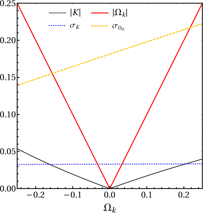
Figure 1: Absolute values and uncertainties of the two curvature quantities $\Omega_{k}$ and $K(z_{l},z_{s})$ plotted vs $\Omega_{k}$. The ratio of the value to the uncertainty is unity where the respective curves cross. The uncertainties are for a single lens system at $z_{l}=0.6$, $z_{s}=1.2$ with fractional distance uncertainties on $D_{\Delta t}$, $r_{l}$, and $r_{s}$ of $\{3\%,1\%,1\%\}$ respectively.

The intersection point between the curvature quantity ($\Omega_{k}$ or $K$) curve and its uncertainty curve determines the lower bound on the measurement of the curvature parameter for a given strong lens system. Due to the scaling discussed above, in fact $\sigma_{\Omega_{k}}/|\Omega_{k}|\approx\sigma_{K}/|K|$ (which we will abbreviate as the inverse signal to noise $S/N$) and so the intersections correspond to nearly the same value of $\Omega_{k}$ that can be distinguished from flatness. For example, the $S/N=1$ for the $\Omega_{k}$ quantity at $\Omega_{k}=-0.15$ or $\Omega_{k}=+0.20$, and the same holds for the $K$ test, for $\{3\%,1\%,1\%\}$ precision. Thus a single such system could distinguish $\Omega_{k}<-0.15$ from $\Omega_{k}=0$ at $S/N>1$.

These results were for a single system, with fixed $z_{l}=0.6$ and $z_{s}=2z_{l}$ so we next investigate the sensitivity to the two redshifts, including the optimum, and the improvement enabled by large numbers of systems delivered by next generation strong lensing, supernova, and BAO surveys.

Considering the redshift distribution, we expect that the raw sensitivity should improve for large $r_{s}$ (i.e. $D$) since this lowers the uncertainty at fixed $\sigma_{D}/D$. However, systems at high redshift would likely be less well constrained observationally and so $\sigma_{D}/D$ would in fact increase. The interplay with the observational accuracy depends on the specific type of measurement, e.g. BAO or supernovae, what type of BAO (e.g. galaxies, quasars, etc.), and survey strategy and specifics and is beyond the scope of this investigation. Instead we will present results fairly generally, taking as a baseline a conservative approach of medium redshifts ($z_{l}\lesssim 0.6$) and discussing the impact of higher redshift observations if they can be accomplished with good accuracy (perhaps in “golden” systems).

Figure 2 plots the S/N in the determination of curvature $\Omega_{k}$ and the K test as a function of the two redshifts $z_{l}$ and $z_{s}$, for the case with $\Omega_{k}=-0.05$. As expected from the previous discussion, the two tests are substantially similar. The highest $S/N$ occurs for the highest $z_{s}$, under the assumption of constant fractional precision. We see that the optimum for a given $z_{s}$ indeed occurs at $z_{l}\approx z_{s}/2$. (This gives $r_{l}$ slightly greater than $r_{l}\approx r_{s}/2$ since by Eq. 8 we want somewhat higher $D_{\Delta t}$ and $r_{l}$ to reduce the error on $\Omega_{k}$.)

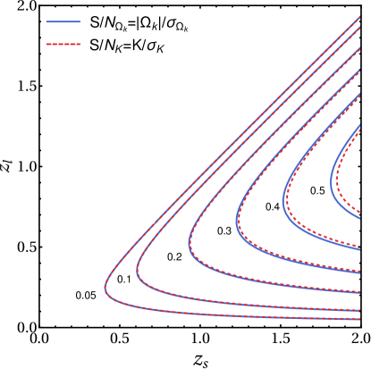
Figure 2: Isocontours of $S/N_{\Omega_{k}}=\mathinner{\!\left\lvert\Omega_{k}\right\rvert}/\sigma_{\Omega_{k}}$ and $S/N_{K}=K/\sigma_{K}$ are plotted in the $z_{s}$-$z_{l}$ plane, for fixed $\Omega_{k}=-0.05$ and $\{3\%,1\%,1\%\}$ fractional distance precision.

Our canonical $z_{l}=0.6$, $z_{s}=1.2$ gives a $S/N\approx 0.3$, so some 10 systems would be required to get $S/N=1$ for distinguishing $\Omega_{k}=-0.05$ from 0. Pushing to $z_{l}=0.9$, $z_{s}=1.8$ could raise the $S/N$ to 0.5, but at the price of longer and more difficult observations to reach the same fractional distance precision.

The redshift dependence of the uncertainty in $\Omega_{k}$ and K estimations is presented in more detail in Fig. 3, for the moment fixing $z_{s}=2z_{l}$ since this gives close to the optimum. As expected the uncertainties decrease for higher $z_{l}$ (and hence higher $z_{s}$, going roughly as $(1+z_{l})^{-4.3}$ for $\sigma_{\Omega_{k}}$ and $(1+z_{l})^{-2.7}$ for $K$. While $\Omega_{k}$ is of course constant with redshift, $K$ increases so $\sigma_{K}/K$ and $\sigma_{\Omega_{k}}/\Omega_{k}$ keep nearly in step over the redshift range of interest. Furthermore, the statistical uncertainties decrease as the square root of the number of systems $n$, so the $S/N$ improves as $1/\sqrt{n}$. We also plot the systematic bias $\delta K$ and $\delta\Omega_{k}$ due to the nonlinearity of the error propagation; these are negligible in comparison to the statistical uncertainties for $n<10^{4}$ and can be controlled further as we discuss below and in Appendix A.

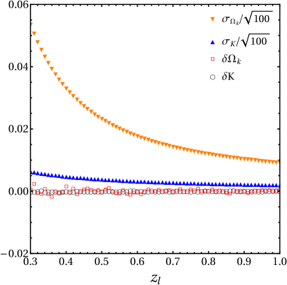
Figure 3: Standard deviations $\sigma_{K}/\sqrt{100}$ and $\sigma_{\Omega_{k}}/\sqrt{100}$ (corresponding to 100 systems) and biases $\delta K=\langle K\rangle-K_{\text{true}}$ and $\delta\Omega_{k}=\langle\Omega_{k}\rangle-\Omega_{k,\text{true}}$ are plotted versus $z_{l}$. The averages are weighted as discussed in the text.

Next we consider ensembles of measurements over a range of redshifts such as would be delivered by next generation surveys. Set A has $z_{l}\in[0.3,0.6]$, representing a medium depth survey, and Set B has $z_{l}\in[0.3,0.9]$, for a deep survey, both with a source distribution $z_{s}=[1.5\,z_{l},2.5\,z_{l}]$. While there is more volume at higher $z_{l}$, the measurements are more difficult; we do not compute a lens redshift distribution, which would depend on survey specifics such as magnitude depth, cadence, etc., but rather sample $z_{l}$ randomly from a uniform distribution in the given ranges. The source redshift $z_{s}$ is then sampled uniformly from its corresponding range. We study results for 100, 400, and 800 systems, to check statistical scaling.

An instantiation of the sets with 100 systems each is shown in Figure 4. For the distances, we sample from normal distributions to incorporate observational uncertainties. For every redshift pair of $z_{l}$ and $z_{s}$, from either Set A or B, we compute $D_{\Delta t}$, $r_{l}$, $r_{s}$ distances and multiply each by a random number drawn from the normal distribution with unit mean and standard deviation set to measurement fractional precisions $\{3\%,1\%,3\%\}$ respectively. This gives realizations of all the simulated data, from which can then be computed the $\Omega_{k}$ and $K$ quantities.

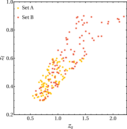
Figure 4: Sets A and B of $N$=100 uniformly distributed $(z_{l},z_{s})$ pairs with $z_{l}$ $\in$ $[0.3,0.6]$ and $z_{l}$ $\in$ $[0.3,0.9]$ respectively, and $z_{s}=(2\pm 0.5)z_{l}$ for each set.

We are particularly interested in the discriminatory power of the estimated quantities to make a statistically significant detection of curvature compared to flatness. This can be thought of in terms of a “signal to noise” ratio, defined as $S/N_{X}=\langle X\rangle/\langle\sigma_{X}\rangle$, where $X$ is either $\Omega_{k}$ or $K$. The ensemble standard deviation is propagated from independent individual measurements by

$$\langle\sigma_{K}\rangle=\frac{1}{\sqrt{\sum\frac{1}{\sigma_{K_{i}}^{2}}}}\ .$$ (10)

For each particular value of $\Omega_{k}$, there is an associated $S/N_{X}$ derived from the ensemble of data. This allows us to investigate several important characteristics: 1) for what range of $\Omega_{k}$ can we disfavor flatness? 2) which test – estimation of $\Omega_{k}$ or the K test – is more incisive?, and 3) how does the estimation scale with data set, i.e. redshift range, number density, and total number?

Figures 5 and 6 show the results. First, note that for small values of $\Omega_{k}$ the $S/N$ is rather linear with $|\Omega_{k}|$, and fairly insensitive to whether $\Omega_{k}<0$ or $\Omega_{k}>0$. Of course, $S/N=0$ for the flat universe since by definition there is no signal of deviation from flatness. Second, the $\Omega_{k}$ estimation and the K test give nearly the same results, as motivated earlier, so we are free to use either (and they do have different error propagation so consistency of results is a good crosscheck). Third, in the most pessimistic of our scenarios (Set A with 100 systems), the data achieves $S/N>1$ for $|\Omega_{k}|>0.025$ and in the most optimistic of our basic scenarios (Set B with 400 systems), $S/N>1$ for $|\Omega_{k}|>0.008$.

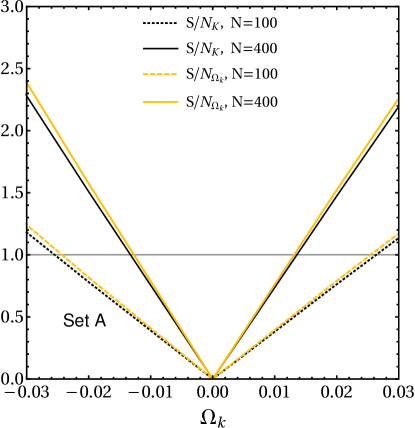
Figure 5: Signal-to-noise ratios $S/N_{K}=\mathinner{\!\left\lvert\langle K\rangle\right\rvert}/\langle\sigma_{K}\rangle$ and $S/N_{\Omega_{k}}=\mathinner{\!\left\lvert\langle\Omega_{k}\rangle\right\rvert}/\langle\sigma_{\Omega_{k}}\rangle$ versus curvature parameter $\Omega_{k}$ for the data realization of Set A, with 100 or 400 systems total. The light grey horizontal line indicates $S/N$=1, and hence the intersection with it gives the constraint on $\Omega_{k}$.

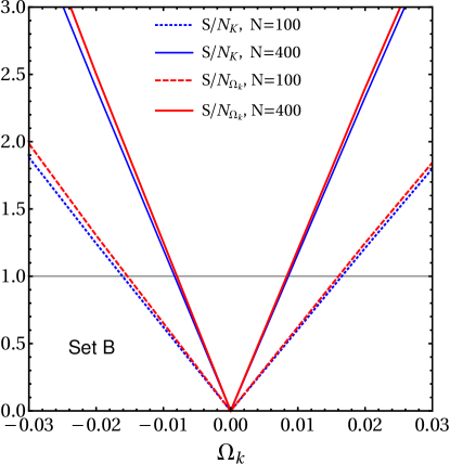
Figure 6: As Fig. 5, for data realization Set B.

As for scaling, the $S/N$ goes as the square root of the total number of data points, but we also see that redshift range plays a strong role. For the same number of systems, Set B provides a $\sim 50\%$ increase over Set A in $S/N$ despite having half the number density of systems. More quantitative detail appears below.

One of the virtues of the K test is that it has a particular predicted redshift dependence, given by Eq. (II). To explore this, we can subdivide the data into redshift bins, e.g. of width $\Delta z=0.1$. For a relatively small data sample this can give large scatter within a bin. While the statistical dispersion is simply the price paid for a modest data sample, one must also pay careful attention to the bias induced by nonlinearity of the error propagation from fluctuations to large uncertainties. We therefore introduce weighting that gives priority to measurements with small uncertainties and reduces the impact of data with large uncertainties.

The most straightforward implementation is inverse variance weighting. We apply this to the K test data, since this is predominantly what we want to subdivide. Defining

$$\langle K\rangle=\frac{\sum\frac{K_{i}}{\sigma_{K_{i}}^{2}}}{\sum\frac{1}{\sigma_{K_{i}}^{2}}}\ ,$$ (11)

where $i$ runs over each data point within the desired subsample (i.e. redshift bin), we find that this greatly ameliorates bias, keeping it much less than the statistical dispersion. We discuss this in detail in Appendix A.

Figure 7 plots the individual redshift bin measurements, with error bars, for a data realization of the optimistic survey of Set B, with 800 systems total. We choose to plot the optimistic case so that the eye can readily discern that the $S/N>1$. For less optimistic cases with $S/N\approx 1$, the eye cannot recognize the pattern in the scatter as easily. In the case plotted, we can see the clear trend of increased deviation of $K$ from zero with redshift, and that it is consistent with the curve expected (Eq. II) from $\Omega_{k}=-0.02$ (the actual input to the realization). In a $\Delta\chi^{2}$ sense, the simulated data discriminates from zero curvature at about $3.5\sigma$, i.e. the estimation of curvature has uncertainty $\sigma_{\Omega_{k}}\approx 0.006$.

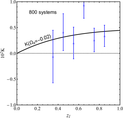
Figure 7: The K test gives a specific redshift dependence in the presence of curvature. The solid curve is the theoretical prediction for $K(z_{l},z_{s})$ versus $z_{l}$ from Eq. (II), for $\Omega_{k}=-0.02$. Points show the results of our simulated measurements $\langle K\rangle\pm\sigma_{K}$ in bins of $z_{l}$ for Set B with 800 systems total. Deviations from $K=0$ point to the existence of curvature, and the redshift dependence both estimates $\Omega_{k}$ and helps separate the signal from systematics.

The trend for other data set realizations is fit fairly well by

$$\Delta\chi^{2}\approx C\,(n/800)^{-1}\ ,$$ (12)

for discrimination of $\Omega_{k}=-0.02$ from flatness by $n$ systems, where $C\approx 12$ for Set B data (long redshift range) and $C\approx 6$ for Set A data (short redshift range). This corresponds to

$$\sigma_{\Omega_{k}}\approx D\,(n/800)^{-1/2}\ ,$$ (13)

where $D\approx 0.006$ (0.009) for Set B (A) respectively. Note the extended redshift range (at constant fractional precision) is worth a factor $\sim 2.4$ in number, i.e. Set B with 330 systems has approximately the same leverage as Set A with 800 systems.

The curvature $\Omega_{k}$ has no redshift dependence and so direct estimation from Eq. (4) does not require any subdivision with redshift. Analyzing the simulated data set Set B with 800 systems total (generated with $\Omega_{k}=-0.02$) as a whole gives $\Delta\chi^{2}=-15$ with respect to zero curvature, a clear signature at the $\sim 3.9\sigma$ level. For this approach, the values of $C$ and $D$ in Eqs. (12) and (13) are 15 and 0.005 for Set B and 7.5 and 0.007 for Set A.

We note that $\sigma_{\Omega_{k}}$ has only a weak dependence on the value of $\Omega_{k}$, with $\sigma_{\Omega_{k}}$ for 800 systems changing by $\sim 10^{-4}$ for a change in $\Omega_{k}$ of 0.02 (and $\sigma_{K}$ is even more insensitive).

In addition to the ensemble evaluation of curvature, we might also like to examine the curvature estimation with redshift, to assure ourselves of its constancy and check for systematics. Performing the same redshift binning as described above, and weighting the estimation of $\Omega_{k}$ as described in Sec. A to control bias due to nonlinear error propagation, we present the results in Fig. 8. The results have very similar $\Delta\chi^{2}$ to the unbinned case, and so again have strong discrimination for the true input model over zero curvature.

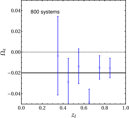
Figure 8: The curvature test in redshift bins has leverage on both estimation of the value of the curvature, and a check on its constancy. The solid curve shows the input value $\Omega_{k}=-0.02$. Points show the results of our simulated measurements $\langle\Omega_{k}\rangle\pm\sigma_{\Omega_{k}}$ in bins of $z_{l}$ for Set B with 800 systems total.

V Conclusion

We sought a robust method of estimating cosmic spatial curvature with three key aspects: 1) it provides an accurate estimate rather than simply a consistency test or alarm, 2) it derives directly from the observations, without taking derivatives or extrapolations of data, and 3) it is as model independent and purely geometric as possible. Two quantities, the direct curvature estimate $\Omega_{k}$ and the K test, satisfied these criteria, using strong gravitational lensing time delay distances and supernova or BAO distances.

Each method could provide a crosscheck of the other, with different error propagation. Furthermore, the K test involves a redshift dependence for the influence of curvature, allowing not only a fit but a verification that the proper functional dependence is satisfied. We examined the error propagation in some detail, demonstrating that not only was bias negligible compared to statistical scatter, but could be further reduced by appropriate weighting or Monte Carlo simulation. The two estimators give similar constraining power, or signal to noise, for data in the range $z_{l}\lesssim 1$.

Carrying out an optimization study, we found that systems with source redshift $z_{s}\approx 2z_{l}$ had the most leverage, close to the natural kernel for strong lensing systems. After an individual redshift analysis to build intuition, we then simulated data sets of various size and redshift range, corresponding to nearer term and next generation distance surveys. We presented analysis of the scaling of the curvature constraints with survey number, number density, and redshift range, finding that the range was the most important, slightly more so than number. For example, Set B had twice the redshift range of Set A and only needed $\sim 40\%$ the number of systems to achieve the same constraining power. However, this assumed the measurement precision could be maintained to higher redshift.

Figures 7 and 8 present illustrations of how applying such curvature analysis to next generation surveys might appear. The K test naturally gives not only a signal of deviations from the zero result of a spatially flat universe but an accurate measurement of the curvature value and a quantitative test of the predicted redshift dependence. The curvature estimator can either apply to the data as a whole, or also divided into redshift slices, allowing a direct check of its predicted constancy with redshift. Again, recall the predictions are model independent, relying only on the Robertson-Walker metric.

One can of course estimate the curvature parameter in a model dependent manner, relying on the Friedmann equations for example. This will generically give tighter constraints, but can be sensitive to the assumed model. For example, misestimation of the dark energy equation of state or the number of effective neutrino species may lead to biases comparable to the desired precision. For our model independent approach, practical application will require careful attention to nuisance parameters in the distance determinations, covariance of measurements, etc. We did not consider Hubble parameter measurements, both because of systematics issues and because even if model independent they are point measures rather than the sort of triangulation we look for in probing the spatial geometry.

Spatial curvature is a fundamental aspect of the universe, and could hold deep clues to inflation and cosmic origins. Estimators formed from the symmetry properties of the Robertson-Walker metric in a model independent manner directly test homogeneity and isotropy. Such methods as we discussed here can be an important complement to other cosmological techniques in exploring the nature of our universe.

Appendix A Dealing with Bias

Like all nonlinear functions of the measurements, formally the K test and estimate for $\Omega_{k}$ are biased due to the nonlinear propagation of measurement uncertainties. However, this is of little real concern in the present case. For next generation data sets of less than 1000 strong lens systems (i.e. measurements of $D_{\Delta t}$), the scatter dominates over the bias. If we look beyond this, there are two straightforward methods for dealing with bias: weighting and Monte Carlo simulation.

The quantity $K$ in the K test involves inverse distances. Sometimes this is actually what is measured, as for BAO transverse angular scales. But if the measurement uncertainties are Gaussian distributed in the distance itself, with mean $D_{0}$ and standard deviation $\sigma_{D}$, then the mean of the inverse distance is $\langle 1/D\rangle=(1/D_{0})[1+(\sigma_{D}/D_{0})^{2}]$. Hence there is a bias of fractional magnitude $(\sigma_{D}/D_{0})^{2}$.

However, we also see the way around this, by weighting the quantity to be averaged such that it appears more linear. This can be accomplished by multiplying $K\sim 1/D$ by $1/\sigma_{K}^{2}$, where the latter is similar to $D^{2}/(\sigma_{D}/D)^{2}$. That is, we expect inverse variance weighting to “debias” $K$. For the $\Omega_{k}$ estimation the situation is more complicated since there are multiple powers of multiple distances. For example, if the first terms in Eqs. (4) and (6) dominate, then the $D$ portion is linearized by weighting by $1/\sigma_{\Omega_{k}}^{1/2}$. Other terms will prefer different weighting. In the end, while informed by such heuristic arguments we rely on purely empirical analysis to determine what weighting is most successful in debiasing $K$ and $\Omega_{k}$, testing for several redshifts and inputs $\Omega_{k}$.

We conclude that inverse variance weighting works well for $K$ and $1/\sigma_{\Omega_{k}}^{0.35}$ for $\Omega_{k}$. Figure 9 and Figure 10 demonstrate the results. The true, input behavior is recovered to excellent approximation. Note for example that the leftmost $K$ point, corresponding to $z_{l}=0.3$, has a systematic bias at the $2\times 10^{-4}$ level, while the statistical dispersion is larger than this as long as we are dealing with $n<10^{5}$ systems at this redshift.

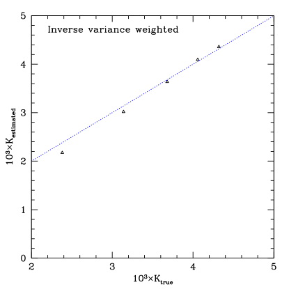
Figure 9: Inverse variance weighting in the K test provides a substantially unbiased result, where $K_{\rm estimated}=\sum(K_{i}/\sigma_{K_{i}}^{2})/\sum(1/\sigma_{K_{i}}^{2})$. The estimates for $z_{l}=0.3$, 0.45, 0.6, 0.75, 0.9 from left to right (triangular points) lie very close to $K_{\rm true}$ (dotted blue line), and the residual bias for this case of $\Omega_{k}=-0.02$ is small compared to the statistical dispersion and the distinction from the flat case $K_{\rm estimated}=0$.

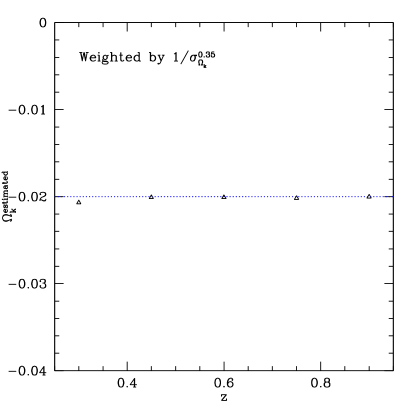
Figure 10: Appropriate weighting on the $\Omega_{k}$ estimator can provide a substantially unbiased result; we find that $\Omega_{k,\rm estimated}=\sum(\Omega_{k,i}/\sigma_{\Omega_{k,i}}^{0.35})/\sum(1/\sigma_{\Omega_{k,i}}^{0.35})$ works quite well. The estimates for $z_{l}=0.3$, 0.45, 0.6, 0.75, 0.9 from left to right (triangular points) lie very close to the true value $\Omega_{k,\rm true}=-0.02$ (dotted blue line).

We emphasize that the weighting, and the results in the figures, should be viewed simply as a demonstration of principle that bias can be reduced. The actual data analysis should employ Monte Carlo simulations of the actual data characteristics. This can furthermore be done iteratively: e.g. subtract the modeled bias for $\Omega_{k}=0$, estimate the new $\Omega_{k}$, resimulate, etc.

References

- Clarkson et al. (2008) Chris Clarkson, Bruce Bassett, and Teresa Hui-Ching Lu, “A general test of the Copernican Principle,” Phys. Rev. Lett. 101, 011301 (2008), arXiv:0712.3457 [astro-ph] .
- Shafieloo and Clarkson (2010) A. Shafieloo and C. Clarkson, “Model independent tests of the standard cosmological model,” Phys. Rev. D 81, 083537 (2010), arXiv:0911.4858 [astro-ph.CO] .
- Mortsell and Jonsson (2011) E. Mortsell and J. Jonsson, “A model independent measure of the large scale curvature of the Universe,” ArXiv e-prints (2011), arXiv:1102.4485 [astro-ph.CO] .
- Sapone et al. (2014) Domenico Sapone, Elisabetta Majerotto, and Savvas Nesseris, “Curvature versus distances: Testing the FLRW cosmology,” Phys. Rev. D90, 023012 (2014), arXiv:1402.2236 [astro-ph.CO] .
- Räsänen et al. (2015) Syksy Räsänen, Krzysztof Bolejko, and Alexis Finoguenov, “New Test of the Friedmann-Lemaître-Robertson-Walker Metric Using the Distance Sum Rule,” Phys. Rev. Lett. 115, 101301 (2015), arXiv:1412.4976 [astro-ph.CO] .
- L’Huillier and Shafieloo (2017) Benjamin L’Huillier and Arman Shafieloo, “Model-independent test of the FLRW metric, the flatness of the Universe, and non-local measurement of ,” JCAP 1701, 015 (2017), arXiv:1606.06832 [astro-ph.CO] .
- Bernstein (2006) Gary Bernstein, “Metric tests for curvature from weak lensing and baryon acoustic oscillations,” Astrophys. J. 637, 598–607 (2006), arXiv:astro-ph/0503276 [astro-ph] .
- Knox (2006) Lloyd Knox, “On precision measurement of the mean curvature,” Phys. Rev. D73, 023503 (2006), arXiv:astro-ph/0503405 [astro-ph] .
- Takada and Dore (2015) Masahiro Takada and Olivier Dore, “Geometrical Constraint on Curvature with BAO experiments,” Phys. Rev. D92, 123518 (2015), arXiv:1508.02469 [astro-ph.CO] .
- Leonard et al. (2016) C. Danielle Leonard, Philip Bull, and Rupert Allison, “Spatial curvature endgame: Reaching the limit of curvature determination,” Phys. Rev. D94, 023502 (2016), arXiv:1604.01410 [astro-ph.CO] .
- Sakr and Blanchard (2017) Ziad Sakr and Alain Blanchard, “Testing General Relativity from Curvature & Energy contents at Cosmological scale,” in Proceedings, 52nd Rencontres de Moriond on Gravitation (Moriond Gravitation 2017): La Thuile, Italy, March 25-April 1, 2017 (2017) pp. 243–246, arXiv:1709.10504 [gr-qc] .
- Witzemann et al. (2017) Amadeus Witzemann, Philip Bull, Chris Clarkson, Mario G. Santos, Marta Spinelli, and Amanda Weltman, “Model-independent curvature determination with 21cm intensity mapping experiments,” (2017), arXiv:1711.02179 [astro-ph.CO] .
- Weinberg (1972) Steven Weinberg, Gravitation and Cosmology (John Wiley and Sons, New York, 1972).
- Shafieloo et al. (2006) Arman Shafieloo, Ujjaini Alam, Varun Sahni, and Alexei A. Starobinsky, “Smoothing Supernova Data to Reconstruct the Expansion History of the Universe and its Age,” Mon. Not. Roy. Astron. Soc. 366, 1081–1095 (2006), arXiv:astro-ph/0505329 [astro-ph] .
- Shafieloo (2007) Arman Shafieloo, “Model Independent Reconstruction of the Expansion History of the Universe and the Properties of Dark Energy,” Mon. Not. Roy. Astron. Soc. 380, 1573–1580 (2007), arXiv:astro-ph/0703034 [ASTRO-PH] .
- Holsclaw et al. (2010) T. Holsclaw, U. Alam, B. Sansó, H. Lee, K. Heitmann, S. Habib, and D. Higdon, “Nonparametric reconstruction of the dark energy equation of state,” Phys. Rev. D 82, 103502 (2010), arXiv:1009.5443 [astro-ph.CO] .
- Holsclaw et al. (2011) T. Holsclaw, U. Alam, B. Sansó, H. Lee, K. Heitmann, S. Habib, and D. Higdon, “Nonparametric reconstruction of the dark energy equation of state from diverse data sets,” Phys. Rev. D 84, 083501 (2011), arXiv:1104.2041 .
- Shafieloo (2012) A. Shafieloo, “Crossing statistic: reconstructing the expansion history of the universe,” J. Cosmology Astropart. Phys 8, 002 (2012), arXiv:1204.1109 [astro-ph.CO] .
- Shafieloo et al. (2012) A. Shafieloo, A. G. Kim, and E. V. Linder, “Gaussian process cosmography,” Phys. Rev. D 85, 123530 (2012), arXiv:1204.2272 [astro-ph.CO] .
- Collett et al. (2012) Thomas E. Collett, Matthew W. Auger, Vasily Belokurov, Philip J. Marshall, and Alex C. Hall, “Constraining the dark energy equation of state with double source plane strong lenses,” Mon. Not. Roy. Astron. Soc. 424, 2864 (2012), arXiv:1203.2758 [astro-ph.CO] .
- Collett and Auger (2014) Thomas E. Collett and Matthew W. Auger, “Cosmological Constraints from the double source plane lens SDSSJ0946+1006,” Mon. Not. Roy. Astron. Soc. 443, 969–976 (2014), arXiv:1403.5278 [astro-ph.CO] .
- Linder (2016) Eric V. Linder, “Doubling Strong Lensing as a Cosmological Probe,” Phys. Rev. D94, 083510 (2016), arXiv:1605.04910 [astro-ph.CO] .
- Paraficz and Hjorth (2009) D. Paraficz and J. Hjorth, “Gravitational lenses as cosmic rulers: m, Λ from time delays and velocity dispersions,” A&A 507, L49–L52 (2009), arXiv:0910.5823 [astro-ph.CO] .
- Jee et al. (2015) Inh Jee, Eiichiro Komatsu, and Sherry H. Suyu, “Measuring angular diameter distances of strong gravitational lenses,” JCAP 1511, 033 (2015), arXiv:1410.7770 [astro-ph.CO] .
- Jee et al. (2016) Inh Jee, Eiichiro Komatsu, Sherry H. Suyu, and Dragan Huterer, “Time-delay Cosmography: Increased Leverage with Angular Diameter Distances,” JCAP 1604, 031 (2016), arXiv:1509.03310 [astro-ph.CO] .
- Liao et al. (2017) Kai Liao, Zhengxiang Li, Guo-Jian Wang, and Xi-Long Fan, “Test of the FLRW metric and curvature with strong lens time delays,” Astrophys. J. 839, 70 (2017), arXiv:1704.04329 [astro-ph.CO] .
- Li et al. (2018) Zhengxiang Li, Xuheng Ding, Guo-Jian Wang, Kai Liao, and Zong-Hong Zhu, “Curvature from strong gravitational lensing: a spatially closed Universe or systematics?” (2018), arXiv:1801.08001 [astro-ph.CO] .
- Aghamousa et al. (2016) Amir Aghamousa et al. (DESI), “The DESI Experiment Part I: Science,Targeting, and Survey Design,” (2016), arXiv:1611.00036 [astro-ph.IM] .