Broadband radio polarimetry of Fornax A, I: Depolarized patches generated by advected thermal material from NGC 1316
Abstract
We present observations and analysis of the polarized radio emission from the nearby radio galaxy Fornax A over 1.28–3.1 GHz, using data from the Australia Telescope Compact Array (ATCA). In this, the first of two associated papers, we use modern broadband polarimetric techniques to examine the nature and origin of conspicuous low-polarization (low-) patches in the lobes. We resolve the low- patches, and find that their low fractional polarization is associated with complicated frequency-dependent interference in the polarized signal generated by Faraday effects along the line of sight. The low- patches are spatially correlated with interfaces in the magnetic structure of the lobe, across which the line-of-sight-projected magnetic field changes direction. Spatial correlations with the sky-projected magnetic field orientation and structure in total intensity are also identified and discussed. We argue that the low- patches, along with associated reversals in the line-of-sight magnetic field and other related phenomena, are best explained by the presence of of magnetized thermal plasma in the lobes, structured in shells or filaments, and likely advected from the ISM of NCG 1316 or its surrounding ICM. Our study underscores the power and utility of spatially-resolved, broadband, full-polarization radio observations to reveal new facets of flow behaviors and magneto-ionic structure in radio lobes and their interplay with the surrounding environment.
Subject headings:
techniques: polarimetric – galaxies: magnetic field – radio continuum: galaxiesI. Introduction
The radio galaxy Fornax A provides an excellent opportunity to study how radio lobes interact with their external environment. The system has undergone a series of dynamical interactions (e.g. Schweizer, 1980; Horellou et al., 2001; Lanz et al., 2010; Beletsky et al., 2011; Iodice et al., 2017) that have triggered episodic activity in the central active galactic nucleus (AGN; Lanz et al., 2010 and references therein) leading to the formation of the iconic radio lobes. However, despite the presence of a weak radio jet in the core of the host galaxy NGC 1316 (Geldzahler & Fomalont, 1984), the system appears to have evolved relatively passively over the past 0.1 Gyr (Iyomoto et al., 1998; Kim & Fabbiano, 2003). The lobes themselves are large and bright, do not have hotspots, do not exhibit the pronounced edge darkening or brightening characteristics of Fanaroff-Riley (FR) I or II sources, and are not connected to the radio core by visible jets. They are quite old (0.1–1 Gyr; Ekers et al., 1983; see also Section VI.1), and their expansion is either frustrated or confined by the relatively sparse Fornax intracluster medium (ICM; Drinkwater et al., 2001; Paolillo et al., 2002; Scharf et al., 2005; Seta et al., 2013). In summary, the Fornax A radio lobes are currently in a relatively mature stage of their evolution, presumably after having interacted more vigorously with the external ICM, and a more spatially-limited ISM (Kim et al., 1998a; Kim & Fabbiano, 2003), in previous epochs.
The lobes host a pronounced network of patches or filaments distinguished by their low apparent emissivity in linear polarization (Fomalont et al., 1989). These structures form the subject of this paper, and we discuss them further below. However we first define some terminology, for the system plays host to a variety of small- to medium-scale structure, in both total and polarized emission intensity (Fomalont et al., 1989). We use the term “low- patches” to collectively refer to patchy/filamentary morphological features that are distinguished by their low level of both fractional and absolute linearly polarized intensity. We use “Stokes filaments” and “polarized filaments” to refer to quasi-linear structures that have high total and polarized emission intensities (respectively) relative to their surroundings. Where we use the word “depolarize” and its derivatives without further qualification or modifying context, we are referring to Faraday depolarization (e.g. see Gardner & Whiteoak, 1966). All of these morphological features are described further in Section V.
The physical cause of the low- patches in Fornax A remains debatable. In other sources, similar structures have been attributed to interactions between the lobe and environment, invoking processes such as shocks (Perley et al., 1984), surface waves (Mason et al., 1988; Bicknell et al., 1990), the formation and evolution of jet-blown bubbles (van Breugel & Fomalont, 1984), cooling instabilities (Simon & Axford, 1967; de Gouveia dal Pino & Opher, 1989), an exterior medium (Clarke et al., 1992), and hydrodynamic instabilities in the magnetized fluid (e.g. Bicknell et al., 1990). In addition, large and complicated Faraday rotation measure (RM) fluctuations across nearby radio lobes have long been observed (e.g. Dreher et al., 1987; Owen et al., 1990), and these may also be related to low-/depolarized patches. While these RM structures are often attributed to the foreground ICM, in some cases the RM structure appears to be generated at the interface between lobes and their surroundings. For example, Carilli et al. (1988) argue that the RM enhancements detected towards the hotspots of Cygnus A are generated as a bow shock is driven into the ICM by the associated radio jet. Venturi & Taylor (1999) argue that RM enhancements observed in the vicinity of the radio jet in 3C 216 arize as a result of jet-ISM interaction in the host galaxy. More recently, Guidetti et al. (2011, 2012) have argued that large-scale, ordered, linear RM structures observed towards several lobed sources are generated at or near the locus of interaction with their surrounding environment.
The past decade has also seen important progress in semi-analytic descriptions, and in hydrodynamic and magnetohydrodynamic simulations, of radio lobes in various environments. These studies (and their forerunners) have uncovered a variety of mechanisms through which low-polarization or depolarized filamentary structure might be generated in and around radio lobes. For example, buoyantly advected thermal plasma from the host galaxy could act as a Faraday-depolarising screen for emission lying in the background (e.g. Churazov et al., 2001; Reynolds et al., 2002; Pope et al., 2010). Alternatively, lobes are generally found to be subject to various hydrodynamical or magneto-hydrodynamical instabilities that generate a complex vortical flow behavior resulting in complex magnetized structure, both internally and at their boundaries (e.g. Bicknell et al., 1990; Brüggen & Kaiser, 2001; Kaiser et al., 2005; Reynolds et al., 2005; Krause & Alexander, 2007; Dursi & Pfrommer, 2008; Dong & Stone, 2009; Huarte-Espinosa et al., 2011; Roediger et al., 2013; Hardcastle & Krause, 2014; Turner & Shabala, 2015; English et al., 2016; and refs. in each). Associated depolarization might then be generated, for example, by foreground turbulence, mixed synchrotron-emitting and Faraday rotating plasmas, or crossed magnetic field lines.
In regards to Fornax A itself, Fomalont et al. (1989) suggested that thermal plasma in the lobes could generate the low- patches through Faraday depolarization, consistent with the buoyant advection scenario described in the preceding paragraph. It is an enticing hypothesis: Detection of thermal plasma in radio lobes has long been sought, since, in addition to encoding information about the interaction history of the system, such material can contribute significantly to the pressure balance, dynamics, and energetics of radio lobes, and can act as seed material for high energy cosmic rays (e.g. Hardcastle, 2010). Whilst early searches for such material did not result in direct detections (McNamara & Nulsen, 2007 and references therein), more recent studies at radio, X-ray, and -ray wavelengths have claimed as much in the lobes of our two nearest radio galaxies — Fornax A (Seta et al., 2013; McKinley et al., 2015; Ackermann et al., 2016) and Centaurus A (O’Sullivan et al., 2013; Stawarz et al., 2013) — though the authors were not able to place strong constraints on the spatial distribution and magneto-ionized structure of this material.
Thus, hypothesising that the low- patches are likely to provide important insights into the nature, physics, and timeline of dynamical processes operating in and around the lobes, we have undertaken a broadband polarimetric analysis of these structures. Our aims are to better constrain their physical origin, and to consider the attendant implications for the magneto-ionized structure of the lobes, and for their history of interaction with the external environment. Our analysis of the main body of the lobes (i.e. outside the low- patches) will be presented in a separate paper (hereafter referred to as paper 2). This paper is organized as follows. We describe our observations and their calibration in section II, followed by explanations of our imaging procedure in section III and our approach to spectropolarimetric analysis in section IV. Our results are presented in section V, then discussed in section VI. A summary of our work and conclusions are presented in section VII. We assume that km s-1 and take the distance to Fornax A to be 18 Mpc (Feldmeier et al., 2007; Stritzinger et al., 2010; but see Cantiello et al., 2013), meaning that an angular diameter of one arcminute corresponds to a linear extent of 5.2 kpc.
II. Observations and calibration
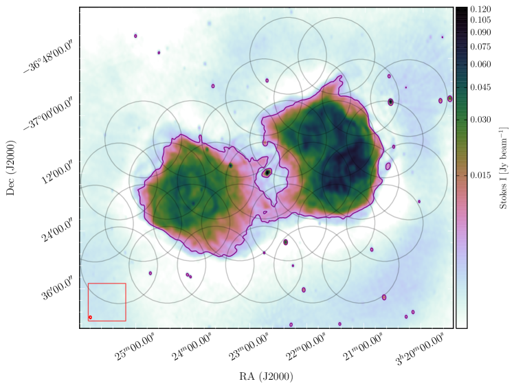
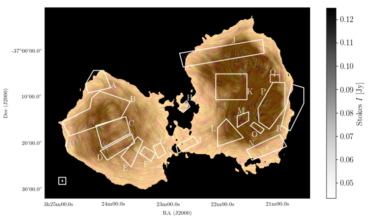
We used the Compact Array Broadband Backend (CABB) correlator on the Australia Telescope Compact Array (ATCA; Wilson et al., 2011) in the ‘CFB 1M’ mode (i.e. 2 GHz total bandwidth, 1 MHz channelization of the continuum) to observe Fornax A in full polarization between 1.1 and 3.1 GHz. We used a 32 pointing mosaic to cover the entire radio galaxy, centered on RA = and Decl. = , and laid out in a regular hexagonal grid with 0.179∘ spacing (see Figure 1). The pointing centers of each beam fall at the one-third power point of adjacent beams at 3.1 GHz. Strictly speaking, the spatial Nyquist-sampling criterion requires adjacent pointing centers to fall at the half-power point, which maximizes sensitivity to highly extended emission. Our mosaic is critically Nyquist-sampled at a frequency of 2.8 GHz instead. This slight under-sampling at the upper end of our frequency band results in only minor non-uniformities in the image sensitivity across the field at these frequencies, and does not significantly increase the net off-axis polarization leakage in the final mosaic, nor substantially limit our ability to detect large scale structure (see further discussion in Section III).
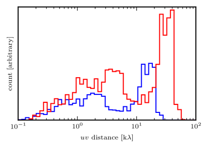
We utilized each of the H75, EW352, 750B, and 6A array configurations to achieve broad coverage at all frequencies (see Figure 2). We observed the mosaic for three separate twelve hour tracks in each of the different east-west array configurations, conducted 2012 November 3rd–5th (750B), 2013 January 11th–13th (EW352), and 2013 March 1st–3rd (6A). An additional six hour track was conducted in the H75 hybrid array, which utilizes antennas on both north-south and east-west tracks, on 2016 August 7th. Excluding overheads and array downtime, each pointing received a total integration time of 130 minutes split over a total of 130 cuts.
Our initial calibration followed standard procedures for the reduction of cm-band ATCA data. Daily observations of PKS B1934-638 were used to calibrate the bandpass response and absolute flux scale. The time-dependent complex antenna gains and on-axis polarization leakage were calibrated using hourly observations of PKS B0332-403. In both cases, independent calibration solutions were derived at 128 MHz intervals through the band, then interpolated across the full band, in order to account for frequency dependent variations in complex gain and polarization leakage (Schnitzeler et al., 2011). Radio-frequency interference (RFI) was flagged iteratively throughout the calibration process using the sumthreshold algorithm (Offringa et al., 2010). All data were flagged between 1.50 and 1.62 GHz, and below 1.28 GHz.
Following the initial calibration, we carried out three cycles of phase self-calibration, as follows. The entire mosaic was imaged jointly through the entire frequency band in 128 MHz chunks using multifrequency synthesis (MFS). We deconvolved these images using the miriad task pmosmem, then convolved the maximum entropy model with a restoring beam. Then, for each imaged frequency band, we split the restored mosaics into primary-beam-weighted images of the individual mosaic pointings using the miriad task demos, then phase-self-calibrated the visibilities corresponding to that pointing and frequency range. For each mosaic pointing, the self-calibration solutions were interpolated across each of the sixteen 128 MHz sub bands spanning the full 1.28–3.1 GHz band, then applied continuously across the total bandwidth. This entire imaging and self-calibration procedure was then repeated twice more.
We estimate that the post-calibration polarization leakage of Stokes into Stokes , , and is no greater than 0.1% of Stokes (e.g. Schnitzeler et al., 2011), and is significantly better directly on-axis when averaged over the band (see e.g. Anderson et al., 2015, 2016) by applying RM synthesis (described below).
III. Imaging
For our spectropolarimetric analysis, we generated Stokes , , , and images of Fornax A throughout the 1.28–3.10 GHz ATCA band. The data were imaged separately in 150 contiguous channels, each covering an equal range in space of m2, spanning a total range of m2. This approach yields a rotation measure spread function (RMSF; Brentjens & de Bruyn, 2005) with the lowest possible sidelobes, possessing a full-width half-maximum (FWHM) of 75 rad m-2. For each imaged channel, the dirty maps were generated using Briggs robust weighting (Briggs, 1995). This weighting scheme represents a trade-off between obtaining high spatial resolution, and achieving sensitivity to large-scale structure in the lobes. The dirty images were deconvolved with the miriad task pmosmem until the RMS noise in the residual image achieved our set threshold of 1.3 times the theoretical value — the lowest factor at which the algorithm reliably converged. The per-channel sensitivity in the resulting images is typically 0.5–1 mJy beam-1 for Stokes , 0.2–0.5 mJy beam-1 for Stokes and , and 0.15–0.3 mJy beam-1 for Stokes , depending on frequency and location in the image. The images were then restored and convolved to a common frequency-independent resolution, re-sampled to a common pixel scale and coordinate grid, then formed into Stokes , , , and datacubes. The images in each frequency channel have five pixels across a synthesized beam (in RA and Decl. respectively) — a resolution well-matched to the scale-size of the patchy depolarization structure that we mean to investigate.
To define the lobe boundaries, and thus the region of interest for our spectropolarimetric analysis, we created a comparatively deep map of the lobes in total intensity by co-adding the re-gridded spectropolarimetric Stokes images. The result is shown in Figure 1. The well-known features of the system are all clearly visible — i.e. the diffuse lobe emission, the bright core / jet region, and a faint radio bridge lying largely to the south of the core that connects the two lobes (see Ekers et al. 1983, Geldzahler & Fomalont 1984, and Fomalont et al. 1989 for detailed descriptions of these features).
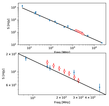
We now comment on whether our spectropolarimetric images suffer from missing flux. Figure 1 gives the impression that this might be the case, given the slight negative bowl apparent around the lobes (though its appearance is exacerbated by the arcsinh stretch employed therein). For GHz-frequency, multi-GHz-bandwidth observations of extended objects, the zero-spacing problem will affect the highest frequencies foremost, and Stokes to a much greater degree than the linearly-polarized emission, since the former is positive-definite, and will generally have a larger characteristic scale size. For our observations though, the shortest effective baseline for an object at zenith for our jointly-imaged data (see Ekers & Rots, 1979) is 9 m, and shorter still once baseline foreshortening is accounted for. This provides us with sensitivity to emission size scales of arcminutes, which is marginally larger than the angular scale of the long axis of the entire system in Stokes . However, a better estimate for the characteristic largest angular scale of the system is – arcminutes, since this range approximately corresponds to the angular size of each lobe, and their separation from one another (Figure 1). Thus, we expect the amount of missing flux to be negligible in all Stokes parameters at all frequencies. To check this, we measured the total flux in our spectropolarimetric Stokes images at several frequencies, then compared these values to measurements of total flux collated from the literature by McKinley et al. (2015), each of which are not expected to suffer from missing flux. The results are plotted in Figure 3, along with a power-law fit to the McKinley et al. data. Our measured total fluxes are consistent with those reported in the literature — if anything, we marginally overestimate the total flux by comparison. Moreover, we were unable to uncover evidence that this situation changed with frequency to better than 10% of Stokes , implying that our fractional Stokes and values (see Section IV) are also good to at least this level. Thus, we do not consider that missing flux affects our results in any important way.
IV. Analysis
Our analysis focuses on the linearly polarized emission from Fornax A. A given state of linear polarization can be represented as a complex vector , which is related to the Stokes parameters and , the polarization angle , the fractional polarization , and the total intensity , as:
| (1) |
Having been emitted from a point , linearly polarized radiation can be Faraday rotated by magnetized plasma along the path to the observer by an amount equal to
| (2) |
where is the polarization angle, is the observing wavelength, and is the Faraday depth, given by
| (3) |
and [cm-3] & [G] are the thermal electron density and magnetic field along the line of sight (LOS) respectively, and the displacement is in units of parsecs.
To remove changes in the linearly polarized intensity caused by simple spectral index effects, we applied our spectropolarimetric analysis to the fractional Stokes quantities and . These were calculated from the Stokes , , and datacubes by:
-
1.
Fitting a power law model to log() vs. log() at each pixel location, then converting this to an model.
-
2.
Dividing the Stokes and values by the model.
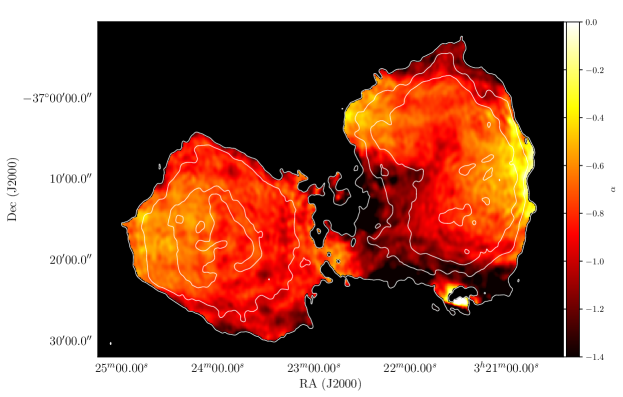
A map of spectral index over the lobes is presented in Figure 4, apparently revealing rich structure. We note that when convolved to a spatial resolution that matches that of the Murchison Widefield Array (MWA) — i.e. arcminutes — the small- and large-scale features apparent in the resulting map are very similar to those observed in spectral tomography maps presented by McKinley et al. (2015) (calculated between 154 MHz and 1510 MHz; cf. Figs. 5 and 6 of that work). McKinley et al. tentatively attributed this structure to imaging and deconvolution artifacts; we propose that it may in fact be real. However, since we find no clear evidence of a spatial relationship between spectral index and fractional polarization in our maps (see Figure 5), we defer a deeper investigation and physical analysis of the spectral index structure to paper 2; here our discussion of spectral index extends only so far as it illuminates the systematic uncertainties in our Stokes fitting, and therefore the calculation of the fractional quantities Stokes and .
The spectral index is precisely determined: At each fitted pixel location for which the band-averaged Stokes intensity was greater than 16 mJy beam-1 (i.e the vast majority of the lobes; see contours in Figure 4), the typical uncertainty in the fitted spectral index is only , while the beam-to-beam variance in spectral index is . This relatively high level of precision is a direct result of the lever arm provided by our broad, densely-sampled 2 GHz bandwidth (see the data and fitting results plotted in Section V.3). We conclude that uncertainties in the Stokes spectral model have negligible impact on our fitting results and analysis. Moreover, a power-law fit provides an excellent description of the Stokes spectral behavior (again, see plots presented in Section V.3). Nevertheless, we tested the the effect of deriving Stokes and by fitting a 2nd degree polynomial to the log() vs. log(), and by dividing Stokes and by Stokes on a point-by-point basis. In both cases, the effect on the Stokes and data and subsequent results was also negligible.
We applied two complementary spectropolarimetric analysis techniques to the Stokes and data. The first is the combined RM synthesis (Brentjens & de Bruyn, 2005) + rmclean (Heald et al., 2009) technique, which generates the so-called Faraday dispersion spectrum (FDS) — a direct reconstruction of the so-called Faraday dispersion function (FDF) from the observational data, itself a complex vector that specifies the intensity and intrinsic emission angle of linearly-polarized emission as a function of Faraday depth along the line of sight. We applied it to the Stokes and datacubes at all pixel locations where the Stokes flux density exceeded 8 mJy beam-1 (see Figure 1). This cutoff level was selected to include the main morphological features of the system, whilst excluding peripheral regions with a low polarized signal-to-noise ratio (S/N). After calculating the FDS at each pixel location, we recorded:
-
1.
: The maximum amplitude of FDS. This provides a measure of the band-averaged fractional polarization (plus Ricean bias, which is insignificant here — see Hales et al., 2012), assuming that the FDS is dominated by emission from a single Faraday depth. As we show in Section V.3, this assumption is often not justified for this object, and in such cases, provides a lower limit on the band-averaged fractional polarization along a given sight-line.
-
2.
: The peak Faraday depth — i.e. the Faraday depth at which FDS is maximized. This represents the Faraday depth from which the bulk of linearly-polarized emission has emerged from along a particular sight line.
-
3.
The noise level in the FDS
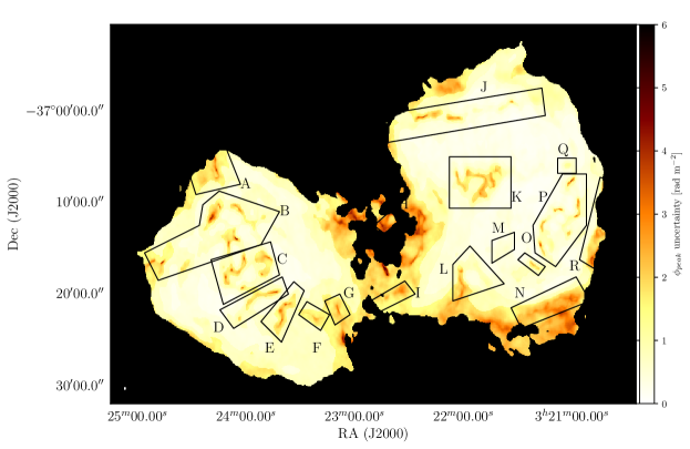
RM synthesis + rmclean provides an excellent estimate of both the band-averaged fractional polarization, (with a typical beam-to-beam variance of for our data), and the peak Faraday depth, with a theoretical uncertainty of rad m-2 for an RMSF width of 75 rad m-2 and a band-averaged polarized signal-to-noise ratio (S/N) — see Figure 19), as well as the range of Faraday depths over which a radio source emits. Moreover, the FDS is calculated without supplying a priori constraints on the nature of the Faraday rotation with physical models, and thereby acts as a point of comparison for the best-fit Faraday rotation models obtained through our second primary analysis technique — (,)-fitting.
(,)-fitting provides a complementary, and in some respects superior (Sun et al., 2015), diagnostic of the nature and structure of magnetized plasmas. This technique has the advantage that physically-motivated models can be fit directly to the polarization data, directly yielding physical constraints on the magneto-ionized structure of sources where a unique best-fit model can be shown to exist. Moreover, (,)-fitting avoids subtle issues associated with the output of RM synthesis and rmclean (e.g. the inability to localize individual rmclean components within the width of the RMSF for sources that are resolved in Faraday depth space).
We fit all combinations of models consisting of one or two polarized emission components, with each described by a variant (described below) of the following function (O’Sullivan et al., 2017, see also Burn, 1966; Sokoloff et al., 1998):
| (4) |
where , , and RM[j] are the initial fractional polarization, initial polarization angle, and rotation measure of the th emission component (respectively), and and characterize Faraday-dispersive effects. The first exponential term in this equation models pure Faraday rotation, the second exponential term models depolarization by a turbulent magnetoionic foreground (i.e. ‘external Faraday dispersion’; but see Burn 1966 and Sokoloff et al. 1998 for discussion of different scenarios in which the depolarization behavior can sometimes differ only subtly from the effect modeled here), while the last term is capable of modeling depolarization behavior from mixed synchrotron-emitting and Faraday-rotating plasma (which we refer to as internal differential Faraday rotation), among other possible scenarios (Schnitzeler et al., 2015).
The different variants of Eqn. 4 just alluded to alternately remove the external Faraday dispersion term, the internal differential Faraday rotation term, and both depolarization terms, resulting in emission components described by Faraday rotation + internal differential Faraday rotation, Faraday rotation + external Faraday dispersion, and Faraday rotation-only respectively. We also fit a three emission component model with all of the terms in Eqn. 4 included, in order to adequately capture the behavior of particularly complex emission.
We fit each such model (which we now refer to as ‘model types’) to the data using the procedure detailed by Anderson et al. (2016). To summarize, we used the emcee sampler (Foreman-Mackey et al., 2013) to identify parameter values that maximize the following likelihood function for polarization data (,) and a model (qmod,i,umod,i) (where is the channel index):
| (5) |
We assigned uniform prior PDFs to all parameters over physically reasonable ranges — i.e. [,) rad for , [0,0.8] for , [-3000,3000] rad m-2 for the RM, and [0,1500] rad m-2 for each of and — and set the PDF to zero over the remaining parameter space.
In order to improve the computational tractability of the (,)-fitting analysis, we down-sampled the Stokes and datacubes to one pixel per synthesized beam area. We then fit each of the model types described above to the (,) data at pixel locations where in the down-sampled cube — i.e. inside the low- patches — and at select pixel locations satisfying to provide a control sample.
We determined the relative merit of the best-fitting model of each type at a given pixel location using the Akaike information criterion (AIC; Akaike, 1974), calculated as:
| (6) |
Here, is the number of fitted model parameters, and is the maximum of the likelihood distribution for a model . For two models and , is exp((AICAICM2)/2) times as likely as to minimize the information lost by under- or over-fitting the data. We considered a model to be strongly favored over a model when AIC AICM2 (i.e. % confidence).
Finally, we note that an explicit and detailed comparison of the output of RM synthesis and (,)-fitting is beyond the scope of this paper — we will present such analysis in paper 2.
V. Results
V.1. The low- patches: Basic morphology and attributes
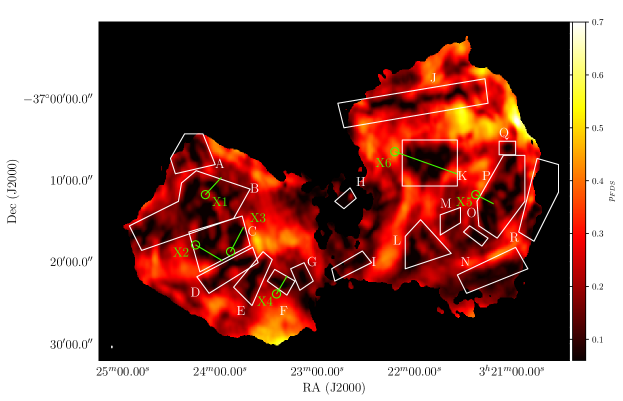
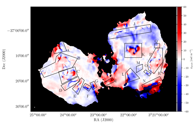
In Figure 5, we present a map of over the lobes. In this and subsequent figures, we use polygons labeled A through R to delineate individual complexes of low- patches, which we refer to as ‘boxes’. The low- patches stand out as the dark regions, though we note that the band-averaged linearly-polarized S/N remains inside the outer lobe boundary. The appearance of these patches in Figure 5 (i.e. in broadband fractional polarization) is much the same as in Figure 1 of Fomalont et al. (1989) (i.e. a narrowband VLA map in linearly-polarized intensity at 1.5 GHz and 14” resolution), and thus, despite the differences in our respective observational setup and capabilities, we are analysing the same structures described by those authors.
The low- patches are resolved in the transverse direction along most of their length, typically by more than three synthesized beam-widths at spatial resolution. This may not be immediately obvious in Figure 5, so in Appendix A (Figures 20 and 21), we present RM synthesis/rmclean-derived maps of and over selected low- patches at resolution. The tapering scheme required to attain this spatial resolution reduces the polarized S/N markedly, precluding the use of these higher resolution images as the main basis of our analysis. Nevertheless, the low- patches are clearly resolved in these maps, and their widths, morphologies, level of fractional polarization, and indeed Faraday depth structure (see Section V.2.1), do not appear to change appreciably despite the substantially increased spatial resolution. Thus, the low- patches are real structures with a physical extent that approximately corresponds to their angular scale in Figure 5.
In contrast to the main body of the lobes, where (expressed as a percentage) is typically and in some places higher than , the value of within the low- patches is typically less than 10%, and reaches as low as 0.8%. Thus, if the low- patches are associated with a Faraday depolarising medium, it must extend close to the lobe surface — i.e. to within a small fraction of one lobe diameter. Were this not the case, synchrotron emission from intervening lobe material would most likely boost the level of observed linear polarization to values more in line with those seen elsewhere in the lobes.
Finally, we note that while the low- patches are not generally associated with known foreground objects (Fomalont et al., 1989), there are two exceptions in the form of small depolarization silhouettes. The first is generated by the Sc galaxy NGC 1310 (Fomalont et al., 1989; Schulman & Fomalont, 1992), and is located in box Q. The second — dubbed ‘the ant’ — is associated with an extragalactic cloud of ionized hydrogen (Bland-Hawthorn et al., 1995). While its morphology is poorly resolved at spatial resolution in band-averaged fractional polarization, it can nevertheless be discerned at the north-west corner of box K. An updated analysis of these structures will be presented elsewhere.
V.2. Spatial-polarimetric analysis of the low- patches
V.2.1 Associated structure in peak Faraday depth
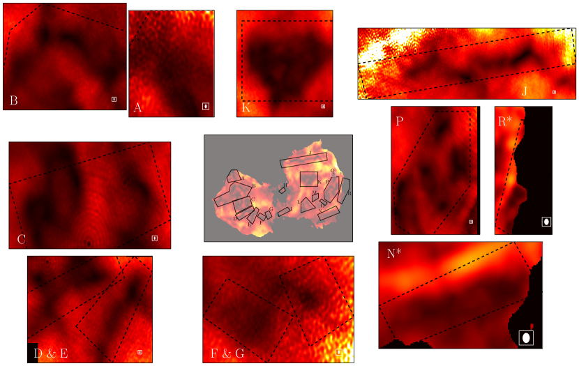
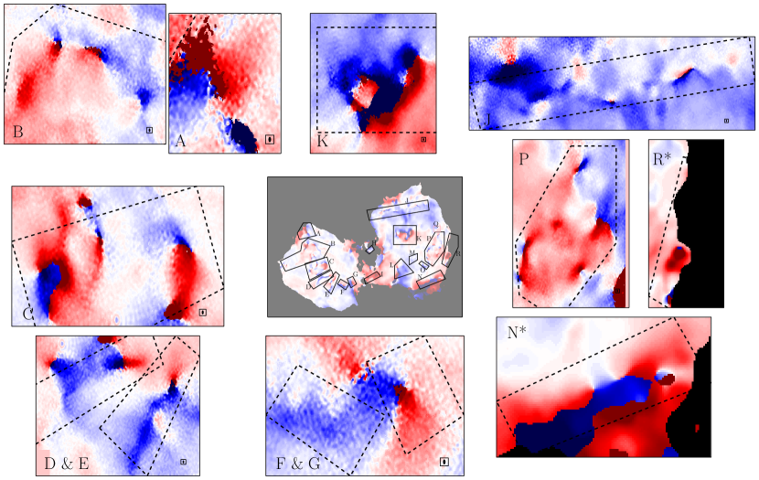
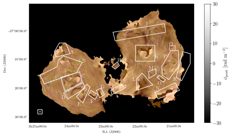
In Figure 6, we present a map of over the lobes. The structure present therein is both obvious and remarkable. It typically manifests as curved, elongated interfaces across which the peak Faraday depth varies rapidly, often changing sign in the process (see boxes C, K, and P for clear examples of this morphology). In some cases though, the interface is not elongated but point-like (i.e. the interface between positive and negative Faraday depth is around one synthesized beamwidth in linear extent — see isolated features in boxes D, E, and L for examples).
From a visual comparison of the and maps (Figs. 5 and 6 respectively), it is clear that a) all of the interfaces in Faraday depth lie within low- patches, generally near their central region or ‘spine’, and that b) the low- patches extend substantially beyond the immediate vicinity of the interfaces alone, and appear to occur wherever either the magnitude of , or spatial gradients in its value, are enhanced relative to the positions in the lobe outside the low- patches. Thus, the patches in question are spatially coincident with distinctive structure in peak Faraday depth, which strongly suggests that they are generated by Faraday effects along the line of sight to the lobes.
The magnitude of the Faraday depth is considerably higher near the interfaces than elsewhere in the lobe — the mean for is rad m-2, and values up to 60 rad m-2 are common. Note that the uncertainty on ranges from –6 rad m-2 in regions with moderate to low fractional polarization (respectively; Figure 19), so that the extreme RM values previously reported towards the system of and rad m-2 by Fomalont et al. (1989) are significantly exceeded, mostly in the immediate vicinity of the interfaces. This discrepancy is probably due to the fact that exhibits considerable frequency-dependent structure at these locations, often including strong depolarization (see Section V.3). Given that the Galactic foreground RM at the location of Fornax A is only rad m-2 (Eqn. 12 of Anderson et al. 2015), the sense of the dominant, regular, line-of-sight component of the magnetic field must change across the interfaces.
V.2.2 Associated structure in the projected magnetic field orientation
The observed relationship between fractional polarization and peak Faraday depth motivated us to consider how these quantities (i.e. and ), as well as morphological features in the Stokes emission, are spatially related to the sky-projected, emission-weighted magnetic field orientation in the lobes. We denote this latter quantity , which we define as:
| (7) |
where and are the values of and predicted by the best-fit polarization model for a given pixel location evaluated at m2. Before continuing, we caution that extrapolating these models from rad m-2 may be unreliable in regions where the frequency-dependent polarization behavior is complex, as it can be near the low- patches (see Section V.3). It is difficult to predict and quantify these effects; future observations at higher frequencies will be required to constrain the intrinsic polarization angle with greater accuracy in such regions.
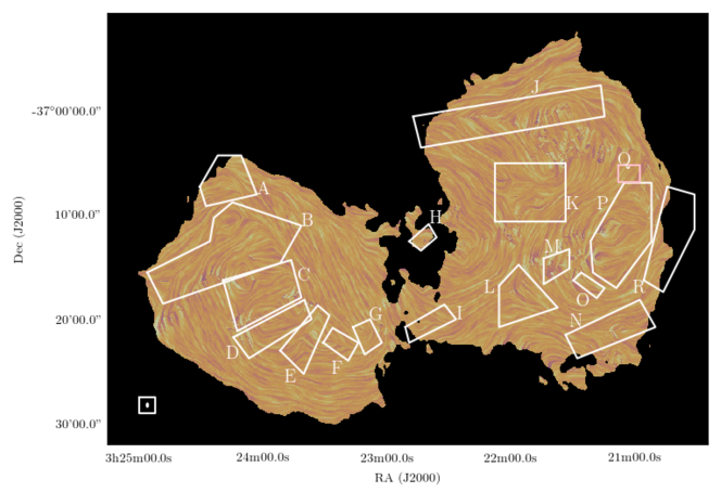
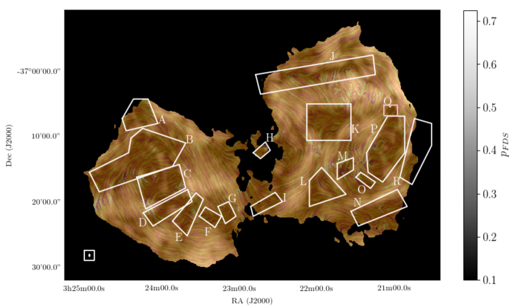
With this caveat, we generated a visualization of using the line integral convolution method (LIC; Cabral & Leedom 1993), whereby a dense collection of streamlines are generated that locally follow , by construction. We present a map of the LIC streamlines in Figure 7. We note that the large-scale structure apparent therein matches that derived by Gardner & Whiteoak (1971) using data from the Parkes telescope at 6 cm. In Figs. 8, 9, and 10, we superpose the LIC streamlines on maps of , , and Stokes , respectively.
Figure 7 shows that exhibits two distinctly different behaviors in the lobes. Some areas possess relatively smooth and coherent structure in on length scales of kpc ( arcminutes) and above, while in others, is knotted into small eddy-like structures or cells on scales of kpc ( arcminutes) and below. These structures are arranged differently in the two lobes: In the eastern lobe, the cells are largely confined to a roughly north-south oriented band (boxes A–F) wherein is predominantly oriented east-west, while elsewhere, predominantly aligns with the projected edge of the lobe. The structure of the western lobes is more complicated: takes on a ‘figure of 8’ shape on the largest scales (with part of the lower loop of the ‘8’ truncated), while prominent small-scale cells in are located above, below, and to the side of the crossing point in the ‘8’ (see boxes K, L, and P respectively). Regardless, it is clear that the low- patches are primarily found in the locations where exhibits this small-scale eddy-like structure (see Figure 8). More specifically, the low- patches are located where the orientation of changes rapidly, and perhaps more intriguingly, in regions that are immediately adjacent to such (and also immediately adjacent bright Stokes filaments; see depolarized patches in boxes B, C for example).
The interfaces in also occur in and around the complicated intersections of streamlines associated with the cells. More precisely, the interfaces often occur where streamlines associated with the meet at oblique angles. It might then be thought that the interfaces are merely artefacts caused by observing emission from crossed magnetic fields in the same synthesized beam. There are several arguments against this however:
- 1.
- 2.
-
3.
Crossed magnetic fields should generate frequency-independent depolarization, whereas we show in Section V.3 that this is not generally what is observed.
Rather, the observed – spatial relationship might represent evidence that the Faraday depth interfaces occur at junctures in the bulk magnetic field structure — and perhaps more speculatively, in bulk flows of material — in the lobes.
In both lobes, emission features in total intensity also coincide with structure in to some extent (see Figure 10), though this is most apparent for the large-scale component of the structure apparent in . Generally, the relationship manifests as an alignment between and the projected edge of the lobes (as is commonly observed; e.g. Laing, 1980; Huarte-Espinosa et al., 2011), and between and the brighter Stokes filaments. The smaller-scale cellular structure in is generally found in between the bright Stokes filaments, and often appears to merge at oblique angles with in the Stokes filaments (see the western regions of boxes B and C for example). It is not clear whether this is a projection effect, or whether different Stokes filaments are interconnected by the magnetic field in this way. Nevertheless, the low- patches appear to be found in-between, and adjacent to, the bright Stokes filaments. Though the precise nature of this relationship is not clear, it nevertheless implies that the process(es) that generate the depolarized patches are in some way linked to the process(es) that generate the bright Stokes filaments.
V.2.3 Cross-sectional analysis
We investigated the magneto-ionized structure across the low- patches / interfaces in more detail by extracting , , and along a number of cross-sections cutting through them. In each case, the data values were extracted at the nearest-neighbor pixel along the cross-section. The cross-sections are indicated on Figure 5, and the extracted data are plotted in Figure 11. We include data from six such cross-sections to supply a representative picture of the observed behaviors. Depending on the orientation of each cross-section, the effective FWHM of the synthesized beam varies between 21 and 27 arcseconds.
The plots firstly confirm that the low- patches are not merely the result of under-resolved monotonic changes in either Faraday depth or intrinsic polarization angle. The degree of depolarization expected in the former case can be calculated using Eqn. 2 of Laing et al. (2008):
| (8) |
where is the intrinsic fractional polarization, RM is the gradient of the RM across the synthesized beam, and is the standard width parameter for a circular Gaussian synthesized beam. At a weighted-mean-wavelength-squared value of 0.025 m2 (i.e. relevant to the fractional polarization outputted from RM synthesis), and for Faraday depth gradients of 10, 20, and 50 rad m-2 across the FWHM of a synthesized beam, we would expect to see depolarization from the maximum level observed in a nearby, off-patch position to 0.98, 0.91, and 0.56 of that maximum value, respectively. The plots of and presented in Figure 11 demonstrate that the level of observed depolarization along each cross-section is generally too large to be explained in this way. Similarly, the spatial gradient in the projected magnetic field orientation does not generally achieve the level of radian per synthesized beam-width that would be required to produce significant depolarization.
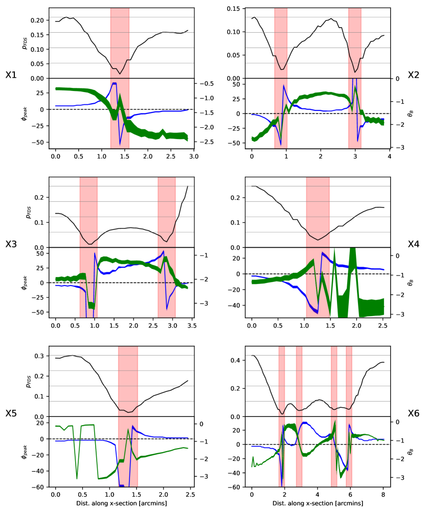
Figures 5 and 6 reveal that complex spatial changes in and are associated with the low- patches, and therefore, the behavior of the , , and over the cross-sections will shed light on the physical processes operating there. Examination of the plots for cross-sections X1–X6 generally reveal that the interfaces in (see Section V.2.1) appear to be approximately coincident with the point of minimum fractional polarization, and appear to form a spine around which broader low- complexes appear. At the interfaces, the Faraday depth jumps by 50–100 rad m-2 on average (and, we note, up to 100s of rad m-2 when this experiment is repeated with the higher-resolution data presented in Figures 20 and 21). At the distance of Fornax A, this implies the existence of a marked change in magnetoionic structure (and where the sign of changes sign, magnetic structure) over linear scales of less than a few kiloparsecs. More often than not, the absolute value of appears to increase increasingly rapidly as the interfaces are approached, but this is not always the case — see for example the curves over cross-sections X4 and X6.
V.3. Spectropolarimetric modeling
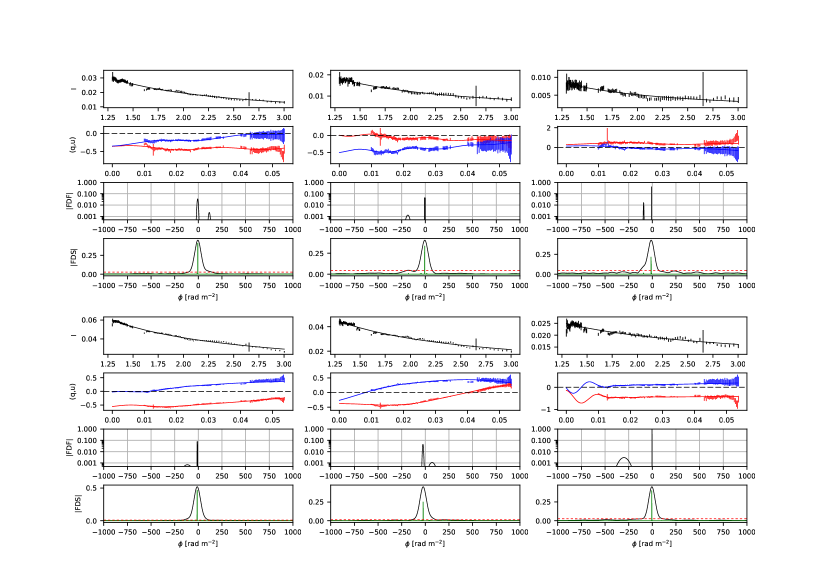
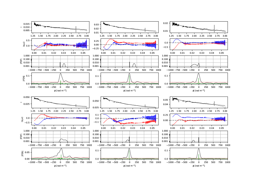
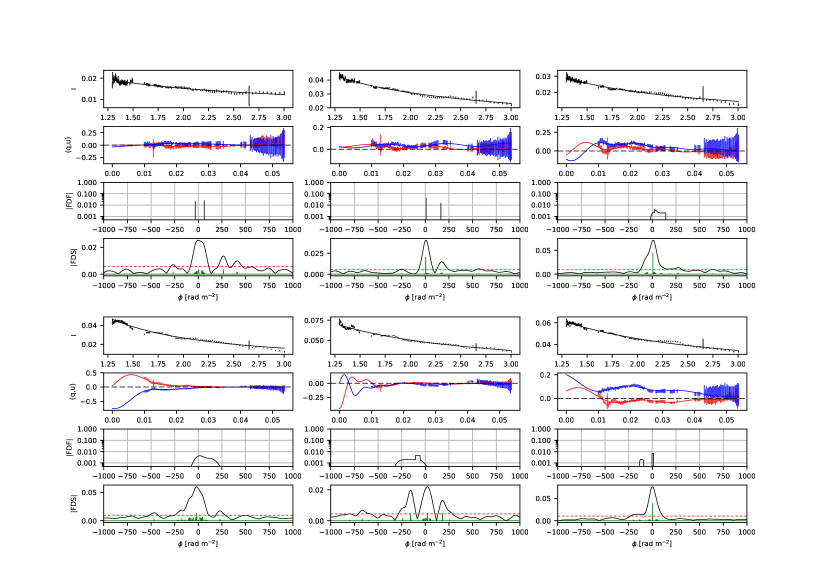
We now describe the results of our (,)-fitting analysis (Section IV). We start by presenting raw spectropolarimetric data and models for a sample of pixel locations. We randomly selected eighteen such locations for this purpose, divided evenly between regions satisfying , , and , which is designed to isolate pixels outside, at the periphery of, and inside the low- patches respectively. The spectropolarimetric data from each location are plotted in Figs. 12–14, while the pixel locations themselves are indicated on Figure 15 (top row). Each of Figures 12–14 consists of a (row column) grid of four vertically-tiled sub-panels. Each location in the grid presented data for one pixel location, with the four panels presenting (from top to bottom) the Stokes spectrum plus best-fit model, the Stokes and data plus best-fit model, the FDF corresponding to this model (e.g. see Anderson et al., 2016; O’Sullivan et al., 2017), and the reconstructed FDS outputted from RM synthesis and rmclean.
Qualitatively, for the central and peripheral locations of the low- patches, the plots reveal that:
- •
-
•
Multiple emission components are generally required in/detected in the model FDF/reconstructed FDS. Typically, each component strongly influences the observed spectropolarimetric behavior.
-
•
The components often emit over a substantial range in Faraday depth, based on the widths of components required in the best-fit model FDF, and the location of rmclean components in the reconstructed FDS
In contrast, outside the low- patches (see Figure 12), it is evident that:
-
•
Stokes and remain greater in magnitude across the entire range
-
•
While some degree of non-sinusoidal frequency-dependent behavior in Stokes and remains, the polarization behavior is generally dominated by single emission components with narrow -widths and low absolute peak Faraday depths
-
•
Where additional components are present in the model FDF, they are comparatively narrow in -space, and contribute a comparatively small amount of polarized flux
These observations generally extend to the full set of numerical results from (,)-fitting. The (,)-fitting results are recorded in Table 1 for the pixel locations plotted in Figures 12–14. Columns 1-11 of the table contain (respectively): The pixel coordinate location of the fitted data, whether the pixel is located outside (denoted ‘O’), at the periphery of (P), or in the spine (S) of the low- patches, the fitted Stokes spectral index, the band-averaged Stokes flux density (denoted ), the best-fit parameter values and their uncertainties for the -th emission component in the best-fit model for , , RM, , and , and finally, the reduced- (denoted ) and AIC values of the best-fit model for the pixel location concerned. We note that the type and number of emission components in the best-fit model can be inferred on the basis of blanked entries in the table. In a separate table (Table 2), we record several statistics that provide a summary of the (,)-fitting results for all fitted pixel locations inside and outside the low patches. Columns 1–8 of Table 2 contain (respectively): The type of region in relation to the low- patches (again, O, P, or S), the number of pixel locations (i.e. independent synthesized beam areas; see Section IV) analyzed in each such region, the proportion of pixel locations in each region that have: (i) a single model uniquely favored by our AIC criteria, (ii) external depolarization terms only in the best-fit model, (iii) internal depolarization terms only in the best-fit model, and (iv) both external and internal depolarization terms in the best-fit model, and finally, the mean values of the fractional-polarization-weighted values of and for the best-fit model over its emission components, which are defined as:
| (9) |
and:
| (10) |
| (1) | (2) | (3) | (4) | (5) | (6) | (7) |
|---|---|---|---|---|---|---|
| Pixel | Location | RM[1,2,3] | ||||
| [mJy beam | [rad] | [rad m-2] | ||||
| (55, 27) | O | -0.93 | 28 | 0.465(0.008),0.041(0.010),-(-) | -1.21(0.02),-1(2),-(-) | -6.9(0.8),110(30),-(-) |
| (55, 41) | O | -0.83 | 15 | 0.46(0.01),0.06(0.03),-(-) | -0.75(0.02),-1.1(0.2),-(-) | -5.8(0.8),-190(10),-(-) |
| (63, 6) | O | -1.19 | 9 | 0.39(0.03),0.1(0.2),-(-) | 0.18(0.10),-2(2),-(-) | -11(3),-100(300),-(-) |
| (119, 55) | O | -0.76 | 52 | 0.564(0.008),0.2(0.1),-(-) | -1.45(0.04),-0.1(0.8),-(-) | -12(1),-0(100),-(-) |
| (127, 55) | O | -0.69 | 37 | 0.47(0.02),0.1(0.2),-(-) | -1.34(0.07),-0.4(0.9),-(-) | -26(3),100(200),-(-) |
| (137, 51) | O | -0.42 | 21 | 0.456(0.003),0.34(0.02),-(-) | 1.53(0.01),-1.2(0.3),-(-) | -3.3(0.5),-200(30),-(-) |
| (29, 47) | P | -0.91 | 12 | 0.22(0.04),0.14(0.02),-(-) | -1.5(0.2),0.6(0.2),-(-) | 130(10),-5(6),-(-) |
| (42, 21) | P | -0.86 | 29 | 0.15(0.01),0.29(0.09),0.12(0.06) | 0.1(0.1),-1.3(0.7),-0.3(0.8) | -5(4),150(80),-200(300) |
| (64, 34) | P | -0.71 | 17 | 0.6(0.1),0.20(0.01),-(-) | -1(2),-1.46(0.09),-(-) | -160(40),-5(3),-(-) |
| (112, 47) | P | -1.01 | 37 | 0.23(0.05),0.3(0.1),0.22(0.07) | 0.3(0.4),-1(2),-0.2(0.4) | -30(20),100(200),-40(90) |
| (119, 61) | P | -0.82 | 50 | 0.164(0.008),0.3(0.3),-(-) | -1.09(0.08),1(2),-(-) | -15(3),-80(70),-(-) |
| (132, 48) | P | -0.47 | 54 | 0.26(0.07),0.163(0.008),0.12(0.05) | -0.9(0.3),0.90(0.02),-1(1) | -30(50),-3.9(0.9),100(300) |
| (15, 29) | S | -0.55 | 18 | 0.034(0.004),0.2(0.3),-(-) | -0.2(0.2),1(1),-(-) | 59(10),200(300),-(-) |
| (33, 34) | S | -0.64 | 38 | 0.047(0.006),0.7(0.3),0.02(0.02) | 0.3(0.2),-1.4(0.7),-1(1) | 10(6),150(70),200(300) |
| (43, 29) | S | -0.81 | 26 | 0.12(0.01),0.27(0.03),-(-) | 0.24(0.07),-1.3(0.2),-(-) | 15(3),88(9),-(-) |
| (111, 47) | S | -1.01 | 36 | 0.26(0.09),0.39(0.07),0.04(0.07) | -1.1(0.2),0.1(0.2),1.1(1.0) | 50(10),-30(20),-500(200) |
| (130, 40) | S | -0.53 | 60 | 0.13(0.01),0.6(0.2),-(-) | -0.1(0.1),-0.9(0.4),-(-) | -78(4),-200(200),-(-) |
| (132, 37) | S | -0.57 | 54 | 0.11(0.02),0.1(0.2),0.11(0.02) | 0.77(0.06),-0.5(0.6),1(1) | 6(3),-300(200),-10(40) |
| (1) | (2) | (8) | (9) | (10) | (11) |
|---|---|---|---|---|---|
| Pixel | Location | AIC | |||
| [rad m-2] | [rad m-2] | ||||
| (55, 27) | O | 5.4(0.7),8(7),-(-) | -(-),-(-),-(-) | 0.62 | -884 |
| (55, 41) | O | 9.6(0.9),19(9),-(-) | -(-),-(-),-(-) | 0.44 | -721 |
| (63, 6) | O | -(-),0(30),-(-) | -(-),-(-),-(-) | 0.46 | -342 |
| (119, 55) | O | 6(2),20(20),-(-) | 4(3),80(60),-(-) | 2.10 | -1117 |
| (127, 55) | O | 4(2),30(50),-(-) | -(-),-(-),-(-) | 0.81 | -1009 |
| (137, 51) | O | 0.1(0.9),71(2),-(-) | -(-),-(-),-(-) | 0.73 | -844 |
| (29, 47) | P | -(-),-(-),-(-) | 42(3),11(5),-(-) | 0.29 | -617 |
| (42, 21) | P | 7(4),20(30),100(300) | 7(4),60(10),0(300) | 0.71 | -962 |
| (64, 34) | P | 76(6),14(2),-(-) | -(-),-(-),-(-) | 0.47 | -763 |
| (112, 47) | P | 7(8),40(10),10(10) | 35(7),60(20),50(20) | 1.39 | -992 |
| (119, 61) | P | -(-),30(10),-(-) | 10(2),50(80),-(-) | 0.53 | -1202 |
| (132, 48) | P | 6(4),11(2),0(200) | 190(60),8(4),100(200) | 1.02 | -1234 |
| (15, 29) | S | -(-),0(200),-(-) | -(-),100(100),-(-) | 0.29 | -818 |
| (33, 34) | S | 2(5),80(40),0(300) | 9(5),90(30),0(200) | 0.43 | -1107 |
| (43, 29) | S | 20(3),-(-),-(-) | -(-),120(2),-(-) | 0.48 | -940 |
| (111, 47) | S | 10(10),40(6),0(200) | 90(10),10(10),0(100) | 0.78 | -1017 |
| (130, 40) | S | -(-),30(10),-(-) | 49.1(0.8),290(90),-(-) | 1.95 | -1188 |
| (132, 37) | S | 2(7),0(200),3(9) | 16(4),100(200),117(5) | 1.21 | -1214 |
| (1) | (2) | (3) | (4) | (5) | (6) | (7) |
|---|---|---|---|---|---|---|
| Location | No. pixels | Proportion single | Proportion | Proportion | Mean | Mean |
| AIC-favored model | one/two/three comps. | external (only)/internal (only)/mixed | ||||
| best-fit model | in best-fit model | physics in best-fit model | ||||
| [rad m-2] | [rad m-2] | |||||
| O | 62 | 0.48 | 0.00, 0.66, 0.34 | 0.16, 0.15, 0.69 | 11 | 24 |
| P | 961 | 0.21 | 0.00, 0.72, 0.28 | 0.12, 0.29, 0.59 | 37 | 61 |
| S | 316 | 0.19 | 0.00, 0.76, 0.24 | 0.11, 0.24, 0.64 | 49 | 75 |
Overall, the best-fit models provide good fits to the data, with mean values in each region of (respectively) 1.61, 0.59, and 0.55. The higher-than-ideal values outside the low- patches appear to indicate that more emission components, or components described by a function other than Eqn. 4, are required to fully encapsulate the behavior of the bright, high S/N polarized emission from these regions. The lower-than-ideal values for the peripheral and spine regions appear to arise as a result of a slight overestimation of the uncertainties on Stokes and . This can be seen in Figs. 12–14, where the scatter between adjacent data points is noticeably lower than the amplitude of their error bars (particularly at high values, where the frequency span of each channel is small — see Section III). This does not affect our analysis or results in any important way — the additional components in the model FDF are clearly required to fit large, systematic changes in Stokes and , which persist over ranges in space that are much larger than the inter-point separation.
For essentially all fitted pixel locations, two or three component models are preferred by the AIC over single component models (column 4 of Table 2). In fact, based on our AIC model selection criteria, single-component models represent a plausible alternative to the best-fitting two- and three-component models at only 6% of pixel locations. Thus, the polarization behaviors in and around the low- patches are mostly inconsistent with simple Faraday rotation by a uniform magnetized thermal plasma in the foreground. Beyond this though, multiple different model types often have AIC values within 10 points of one another (column 3 of Table 2) — for these pixel locations we cannot identify a unique best fit model with a high level of confidence. Inconveniently but unsurprisingly, this is more often the case in the spine and periphery of the low- patches than outside them, owing to the heavily reduced fractional polarization in these regions. Substantially more sensitive observations would be required to break these degeneracies.
While we often fail to identify a single best-fitting model type, we can look for evidence that a particular type of depolarization physics (e.g. external Faraday dispersion, internal differential Faraday rotation) is uniquely associated with the low- patches. We took the model type with the lowest AIC value for each pixel (the most strongly favored best-fit model type, if not a uniquely favored best-fit model type), and classified it as having Faraday rotation only (the terms containing and in Eqn. 4 are equal to one for all emission components), external dispersion only (the term containing in Eqn. 4 is equal to one for all emission components), internal differential Faraday rotation only (the term containing in Eqn. 4 is equal to one for all emission components), or mixed (each of the and terms in Eqn. 4 are not equal to one for at least one emission component). We note that in reality, the generality of Eqn. 4 ensures that ‘mixed’ models describe a wide range of polarimetric behaviors that do not strictly conform to the internal or external mechanisms. Thus, a ‘mixed’ designation does not imply that the precise internal and external depolarization mechanisms modeled by the terms in this equation are necessarily in operation, either separately or together. With that said, we find no evidence to link specific types of depolarization physics to the low- patches (column 5 of Table 2). This strongly suggests that the magneto-ionized structure of the low- patches and their surrounds is complicated: The observed depolarization results from the combined effect of multiple interfering emission components, and various poorly-constrained depolarization mechanisms acting on this emission.
Nevertheless, we can readily determine the characteristic range of Faraday depths and width in Faraday depth space that different components in the best-fit models emit over. The mean values of and (see Eqns. 9 and 10) over the analysed pixel locations are recorded in columns 6 and 7 of Table 2, broken down by region. In general, the locations outside the low- patches have comparatively low values of and , where the fits are well-constrained by the data. The value of ranges up to 32 rad m -2 with an average value of 24 rad m -2, and a typical uncertainty of rad m -2. ranges up to 60 rad m -2, with an average value of 11 rad m -2, and a typical uncertainty of rad m -2. For the peripheral locations in the low- patches, ranges up to 90 rad m -2 with an average value of 61 rad m -2, and a typical uncertainty of rad m -2. The value of ranges up to 314 rad m -2, with an average value of 37 rad m -2, and a typical uncertainty of rad m -2. For the pixel locations in the spine of the low- patches, ranges between 7 and 96 rad m -2 with an average value of 75 rad m -2, and a typical uncertainty of several 10s of rad m -2. The value of ranges up to 330 rad m -2, with an average value of 49 rad m -2, and a typical uncertainty of 10 rad m -2.
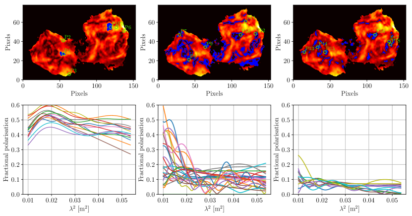
Having described our modeling results, we now attempt to isolate and display characteristic spectropolarimetric behaviors associated with the low- patches. To do so, we once again distinguish between pixels located outside, at the periphery of, and inside the low- patches, according to the inequalities on previously discussed. We indicate each such region in blue on maps of the lobes in columns 1–3 of the upper row of panels in Figure 15 respectively. In the lower row of panels, we plot curves for the best fit polarization model at a set of pixel locations randomly drawn from the highlighted blue regions — one in every four, 40, and 20 pixel locations outside the low- patches, at the periphery of the patches, and in the spine of the patches respectively. Moving from the left-most to right-most column (i.e from regions outside the patches to regions in their spine), the plots of reveal a clear progression of behavior from higher to lower band-averaged fractional polarization. As discussed above, this is associated with the presence of multiple emission components emitting over a range of Faraday depths, and thus the low- patches are generated by Faraday depolarization. The central low- patch locations exhibit the heaviest depolarization over the broadest frequency ranges, which is unsurprising. However, in many cases is not completely depolarized over the entire band, and at m2, there is some indication on an up-tick in fractional polarization towards shorter wavelengths for locations near the spines of the low- patches. We also note that for the peripheral locations, the best-fit models often depolarize over the band, from fractional polarization values similar to those seen outside the low- patches, to values more characteristic of those seen near their spines. Once again, this strongly suggests that it is Faraday depolarization operating in the low- patches.
In general however, this depolarization behavior is not monotonic but oscillatory, meaning that we are not observing the action of a turbulent foreground screen (Burn, 1966), but rather the presence of mixed synchrotron-emitting and Faraday-rotating material, and/or interference effects generated by multiple emission components. Comparing the behavior in the peripheral and central regions of the low- patches, we see this oscillatory depolarization behavior in both cases. However, compared to that for the central regions, the data for the intermediate regions appear to have a greater amplitude of oscillation on average.
In summary, (,)-fitting reveals that:
-
1.
Strong, oscillatory (as a function of ) depolarization is often observed towards the low- patches. This is not consistent with pure Faraday rotation, or with frequency-independent depolarization. It implies that a Faraday-rotating plasma exists along the line of sight which possesses a comparatively complicated magneto-ionized structure.
-
2.
It is rarely the case that is well-constrained to have a high value while is well-constrained to have a low value, or vice versa. Thus, in general, the behaviors cannot be uniquely attributed to either external Faraday dispersion or internal differential Faraday rotation — again, the depolarising medium must have rather more complex structure.
-
3.
The amount and character of the depolarization changes in a systematic way moving from ‘off-patch’ positions towards the central spine of the low- patches. Secondary emission components in the FDF/FDS increasingly dominate the spectropolarimetric behavior. The differential Faraday depths and dispersions of these components tend to increase from typically rad m -2 in the lobe body, to several tens of rad m -2 in the peripheral regions, and somewhat higher still in the inner regions of the low- patches.
VI. Discussion
VI.1. Basic properties of the Fornax A lobes
Our discussion makes use of the following basic lobe properties, which are taken from the literature or measured from our data.
VI.1.1 Sizes
NGC 1316, the host galaxy of Fornax A, lies at a distance of 18 Mpc (Feldmeier et al., 2007; Stritzinger et al., 2010), so an angle of one arcminute corresponds to a projected linear distance of 5.2 kpc. The Fornax A radio lobes range between 20 and 28 arcminutes in projected angular diameter (Figure 1), corresponding to –150 kpc in projected linear extent. We estimate their combined volume to be cubic parsecs. The largest angular scale (LAS) of the system is arcminutes, corresponding to 260 kpc. The typical projected width of a low- patch (i.e. the peripheral and inner regions defined in Section V.3) is kpc, whilst their typical lengths and spine-to-spine separation are –40 kpc and –20 kpc respectively (Figure 5).
VI.1.2 Age
VI.1.3 Thermal plasma content and environment
To successfully model X-ray emission from the Fornax A lobes, Seta et al. (2013) required an emission component from thermal plasma with an electron density cm-3 and total mass of , where the volume filling factor is constrained to be from the inferred cooling timescale. We assume this plasma exists and is dominated by ionized hydrogen and helium nuclei with a typical ICM abundance ratio of 9:1 (respectively), and thus a mass density of , where is the mass of a proton.
The Fornax cluster consists of a main component centered on the cD galaxy NGC 1399, and in-falling subcluster to the southwest centered on NGC 1316 (Drinkwater et al., 2001). The main cluster ICM has been studied in detail: It possesses a central thermal electron density of cm-3 (cluster contribution only), and of gas enclosed inside a 100 kpc radius (Jones et al., 1997; Paolillo et al., 2002). The subcluster ICM has not been studied in similar detail. Seta et al. (2013) implicitly derive cm-3 around Fornax A, by extrapolating a beta-model of the main cluster atmosphere from X-ray measurements at cluster-centric radii of 35–280 kpc (made by Jones et al., 1997) to the 1.5 Mpc main-cluster-centric radius of Fornax A. The uncertainty in the extrapolated value is compounded by the fact that the south-west subcluster is relatively massive in its own right. It contains a total mass of — at least a third the mass of the main cluster — with a probable gas fraction of % (Dvorkin & Rephaeli, 2015), and other indications that it is gas-rich, such as member galaxies experiencing a high ongoing rate of star formation (Drinkwater et al., 2001). Thus, we suggest the aforementioned estimate of the ICM density near Fornax A is probably too low.
VI.1.4 Magnetic field
Previous studies have found that the average magnetic field strength in the lobe body () falls in the range 1–4 G (Kaneda et al., 1995; Tashiro et al., 2009; Seta et al., 2013). Most recently, McKinley et al. (2015) derive a value of () G through precise simultaneous modeling of synchrotron radio emission and inverse Compton-scattered X-ray emission.
VI.2. Summary of our key results
Any proposed explanation for the low- patches must account for, or at least be consistent with, the following key observations:
-
•
That the low- patches are (a) spatially-resolved, (b) centered around enhancements in the value of of typically up to 50 rad m-2 (and sometimes greater), (c) centered around reversals in the sign of , and (d) located in regions where the sky-projected magnetic field orientation exhibits complicated eddy-like structure (though see our caveat in Section V.2.2).
-
•
That complex polarization models are generally required to reproduce the detailed depolarization and repolarization behaviors observed towards the low- patches, including the need for multiple Faraday-rotated emission components, possessing differential Faraday depths and dispersions of typically several 10s, and up to 100s, of rad m-2 (Section V.3)
-
•
That the low- patches exhibit very low values of fractional polarization, implying that the depolarising medium must either reside at, or extend to within a small distance of, the lobe surface (as opposed to being limited in extent to a small volume deep within the lobe; see Section V.1).
VI.3. On the Faraday depth structure associated with the low- patches
Arguably, the most remarkable aspect of our observations is the Faraday depth structure observed towards the low- patches — specifically, that generally reverses sign across the central spine of these regions, while increases systematically as these interfaces are approached.
The sign-reversals observed in are significant. Where they occur, the magnitude of the change in is typically 50–100 rad m-2 over linear scales of kpc or less (Section V.2.1) — much larger than the rad m-2 Galactic RM foreground contribution in this area. This implies that structure in the LOS-projected magnetic field is an important causal factor for the observed Faraday depth structure.
The magnitude of the enhancements in are difficult to explain using the (lobe-averaged) values for (for ) and provided in Section VI.1, which for a fully regular field, will generate only rad m-2 over the width of a typical low- patch. This is about an order of magnitude below that required. In principle, the lobe-averaged and values could generate the required amount of Faraday rotation over path lengths of kpc, but this would require a coherent, regular magnetic field to exist throughout almost the full depth of the lobes. While this might plausibly be the case in parts of the eastern lobe (see Figure 7), the enhancements and low- filaments are not located there, but rather in places where the projected field is knotted on smaller scales (Section VI.2). Thus, it must be that either (a) , , or both in combination are a factor of 10– higher than the lobe-averaged values towards the low- patches, assuming that Faraday rotation occurs over a path length equal to the typical width of a low- patch, or if we relax this last assumption, that (b) local increases in , , and the magnetic field coherence length all act together to produce the required Faraday depths/dispersions.
In either case, we conclude that the low- patches and their associated Faraday depth structure must be generated by regions in the lobes where the local electron density and/or magnetic field strength is elevated above the lobe average(s). We note that McKinley et al. (2015) and Ackermann et al. (2016) reached a similar and potentially related conclusion — namely, that the Fornax A lobes must contain relatively dense thermal plasma agglomerations, in order to successfully explain details of the (Stokes ) radio, X-ray, and -ray emission from the lobes. We discuss the possible physical nature of this magnetized substructure in Section VI.5.
VI.4. Mass, location, and source of the thermal plasma associated with the low- patches
We can estimate the minimum mass of thermal plasma associated with the low- patches in a general way, as follows. The peak Faraday depth of a column of thermal electrons threaded by a uniform magnetic field is (e.g. Heiles & Haverkorn 2012; Anderson et al. 2015):
| (11) | |||||
where is the strength of the magnetic field projected along the line of sight [G], and is the electron column density in units of cm-2. Taking the map presented in Figure 5, then masking out regions where and which fall outside boxes A–G, I–M, O, and P, the solid angle occupied by the low- patches is square arcseconds. This corresponds to a projected area cm2 at the distance of the lobes. Assuming the conversion factor between thermal electron density and plasma mass density given in Section VI.1.3, the total mass of material in the patches is roughly:
| (12) |
Assuming the low- patches are characterized a typical Faraday depth , then combining Eqns. 11 and 12 after solving for , yields:
| (13) |
from which we get , using rad m-2 (Section V.2.1) and (though our conclusions from Section VI.3 should be kept in mind here). In fact, the true mass is likely to be higher than this, since our mask will tend to exclude material lying at the far side of the lobes, and the calculation assumes the magnetic field is oriented along the LOS with no reversals. On the other hand, if the enhancements in are primarily related to local enhancements in the magnetic field strength (Section VI.3), the required plasma mass is reduced in proportion. Nevertheless, we can compare the value as stated with existing observational results in this area. Interestingly, if we split our calculated mass evenly between the two lobes, it agrees with the Seta et al. estimate for the western lobe if , which is consistent with the limits that they place on this parameter (see Section VI.1.3). If we note the projected area occupied by the low- patches and model them as cylindrical regions viewed in projection, their associated volume is cubic parsecs, yielding , which is obviously comparable. Thus we suggest that the thermal material detected by Seta et al. may in fact be associated with the low- patches. Future high-resolution X-ray observations can confirm or refute this. Moving beyond Fornax A, similar thermal plasma masses are found to be associated with the buoyant lobes of other radio galaxies — e.g. Simionescu et al. (2009); Kirkpatrick et al. (2009); Salomé et al. (2011); Werner et al. (2011); McNamara & Nulsen (2012); O’Sullivan et al. (2013); Russell et al. (2017).
Where in the system is this material located, and from where does it originate? It must be associated with the lobes themselves, or we could not explain the observed relationship between the low- patches and structure in the projected magnetic field orientation and Stokes filaments (Section V.2.2). Direct entrainment of the ISM/ICM in the radio jet cannot provide the required mass transport rate (Laing & Bridle, 2002; Seta et al., 2013). One possibility suggested by simulations is that radio bubbles lift and mix thermal plasma into themselves through a combination of buoyant motion and large-scale Rayleigh-Taylor (R-T) instabilities (e.g. Churazov et al., 2001; Reynolds et al., 2002; Pope et al., 2010; Weinberger et al., 2017). The advected plasma masses therein typically range up to M⊙ per lobe. This may be capable of satisfying our requirements, though we note that more material can be probably be lifted through multiple episodes of AGN activity (e.g. O’Sullivan et al., 2013; Russell et al., 2017), by magnetic fields that increase coupling between gas phases in and around the lobes (e.g. Russell et al., 2017), or by additional hydrodynamic forces generated by certain buoyant flow behaviors (Pavlovski et al., 2007). For this scenario, an open question is whether NGC 1316 contained sufficient thermal mass to raise into the lobes to begin with — Forman et al. (1985) and Kim et al. (1998b) find that the total mass of gas in the host is now just . However, the system has also experienced significant merger and interaction events since the formation of the lobes (Mackie & Fabbiano, 1998; Horellou et al., 2001; Beletsky et al., 2011), which may have stripped gas from the host after the lobes formed.
While we favor the advection scenario just described, a plausible alternative is that the ICM previously-displaced by the lobes has begun to intrude back into them via Rayleigh-Taylor (R-T) instabilities (Alexander, 2002; Pizzolato & Soker, 2006; Stone & Gardiner, 2007a, b). Indeed, Seta et al. (2013) have already proposed that this might be the origin of the thermal material in the western lobe. However, their estimate of the thermal plasma density in the lobes is a factor of five greater (more, if ) than their estimate of that in the surrounding ICM (Section VI.1.3). For the R-T mechanism to be viable then, the ICM must cool and condense significantly after penetrating the lobes, or otherwise, the true ICM density around Fornax A must be higher than they project, as we have already discussed (Section VI.1.3). We explore the viability of the R-T scenario further in Section VI.5.2.
Finally, we note that the majority of low- patches appear to sit in a curved lane running through the system, extending from region P in the western lobe, through regions O, M, L, and I, and from there into the eastern lobe through regions G, F, E, D, C, B, and A. This feature is striking, and motivated us to consider whether a more exotic and inherently anisotropic process may have transported the thermal material into the lobe interior, such as the Bondi-Hoyle wake or stripped ISM of an external orbiting galaxy, or jet-induced mixing at the lobe-ICM boundary (e.g. Wilson, 1989; Norman & Balsara, 1993). Both of these possibilities seem unlikely: In the former case, because there are no sufficiently massive galaxies nearby, while in the latter, because there is no evidence of a strong jet having recently operated in the system (Section I). Instead, we suggest that the arrangement of depolarising material is more likely to have been generated by vortical flow behaviors in the lobe, combined with the intrinsic axisymmetry of the system (e.g. Brüggen & Kaiser, 2001). This idea is related to the model that we propose in Section VI.5.
VI.5. The mechanism that produces the low- patches and associated Faraday depth structure
The most significant challenge posed by our results is that of explaining all of the observed interrelationships between the low- patches, enhancements in the magnitude of the peak Faraday depths and associated sign-changes in such, the complex frequency-dependence of the linear polarization signal, and structure in the sky-projected magnetic field orientation (summarized in Section VI.2). We now evaluate several physical mechanisms that represent, in our view, the most plausible means of producing the required couplings.
VI.5.1 Kelvin-Helmholtz instabilities
For buoyant radio lobes rising through a surrounding ICM, a velocity shear will be set up across the lobe-ICM interface, and Kelvin-Helmholtz (K-H) instabilities may form. Considering the observational implications of a magnetic field embedded in these flow structures, Bicknell et al. (1990) proposed that this mechanism may give rise to the RM/depolarization bands observed towards some radio lobes. Modern generic simulations of the K-H instability confirm the basic plausibility of this connection, while somewhat modifying the underlying physical picture. In summary, they show that regular, coherent magnetic field structures can be pulled into the base of K-H vortices, while turbulence and magnetic reconnection events act to form a highly complex magnetized medium inside the vortex itself (Obergaulinger et al., 2010; Karimabadi et al., 2013; Ma et al., 2014 and refs. therein).
To date, simulations of lobe-ICM interfaces specifically have lacked the numerical resolution to track dynamically important microphysical effects in the vortex region (Karimabadi et al., 2013). Nevertheless, they suggest that this interface can become K-H unstable (e.g. Huarte-Espinosa et al., 2011; Weinberger et al., 2017), including in poor cluster environments (Hardcastle & Krause, 2014; English et al., 2016), but that this is sensitively dependent on factors such as the current state of jet operation (e.g. Pizzolato & Soker, 2006; Sternberg & Soker, 2008), the magnitude of viscous damping effects (e.g. Reynolds et al., 2005; Kaiser et al., 2005; Roediger et al., 2013), and the detailed magnetic field configuration of the lobes and that of their environment (e.g. Kaiser et al., 2005; Krause & Alexander, 2007; Ruszkowski et al., 2007; Dursi & Pfrommer, 2008; Dong & Stone, 2009; English et al., 2016).
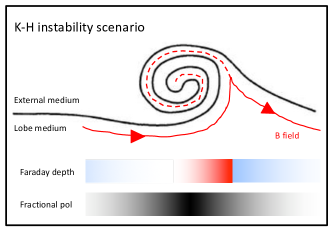
We are unaware of simulations that are currently capable of generating detailed global maps of Faraday depth and depolarization arising from K-H instabilities in realistic lobe environments. Nevertheless, if such instabilities did form at the lobe-ICM interface, then broadly following Bicknell et al. (1990), we suggest that:
-
1.
In regions where the crest of a K-H wave is viewed from above (i.e. the part of the flow feeding into the vortex), the direction of will show a rapid reversal.
-
2.
A complex mixture of Faraday-active material will form in the K-H vortex, potentially Faraday-depolarising emission from the background. Such regions will be spatially correlated with the regions described in the previous point.
-
3.
Waves should appear on the lobe edges as well as on the face, and in the former case, the characteristic projected scale height of the resultant depolarization structure should be one-third of the inter-low--patch distance on the lobes face (Bicknell et al., 1990).
The proposed scenario is depicted in Figure 16. We suggest that the sign-reversals in (Section V.2.1), the spatial coupling between such reversals and the low- filaments (Section V.2.1), and the /depolarization structure observed in boxes A, N, and R of Figures 5 and 6), are qualitatively consistent with this scenario. Moreover, magnetic fields are naturally amplified in K-H vortices, providing a possible means through which substantial Faraday depths can be generated over relatively short path lengths.
The crux of the issue is whether the magnetic fields at the lobe-ICM interface are simultaneously strong enough to generate the required Faraday depths, but weak enough to render the lobe-ICM interface vulnerable to the instability. The former point has been discussed in Section VI.3, noting that the scale-height of a K-H wave will be similar to the widths of the low- patches (as can be deduced from the scale-lengths provided in Section VI.1.1, and the relationship between the wavelength and heights of K-H waves provided by Bicknell et al. 1990).
Addressing the second point, linear stability analysis shows that lobe-ICM interface is stable against K-H instabilities when the Alfvén number (i.e. the ratio of the shear-to-Alfvén velocities) satisfies (e.g. Chandrasekhar, 1961; Obergaulinger et al., 2010):
| (14) |
where is the shear velocity between the two flows, and is the mass density of the lighter of the two mediums. We use cm s-1 (Section VI.1), implicitly assuming that the lobes act like a vortex ring, continuing to exhibit vortical flow even if they have ceased to rise buoyantly (e.g. see Churazov et al., 2001). The large-scale ‘swirling’ morphology of the lobes would seem to support this. For values of , (), and the assumed plasma composition taken from Section VI.1, we have — i.e. the interface is K-H stable.
To achieve instability (at least initially, and prior to the onset of non-linear stabilization/disruption effects — see Frank et al., 1996; Obergaulinger et al., 2010), or must be higher by factors of eight and 64 respectively, or a factor of eight lower. A factor-of-eight increase in is not plausible, not least because this would require the lobe to be moving supersonically through the ICM (e.g. see Machacek et al., 2005). The second possibility, and the third possibility in combination with our prior constraint on the value of the product , imply that cm-3 and cm-3 in the K-H-active layer respectively. In the diffuse Fornax cluster gas though, such high plasma densities are found only in the central arcminute of NGC 1399 — the cD galaxy of the main cluster. Thus the K-H scenario seems unlikely, even in the absence of other difficulties, such as its apparent inability to explain the spatial coupling between the projected magnetic field structure of the lobes and the and low- patches.
VI.5.2 Rayleigh-Taylor instabilities
Studies by Alexander (2002); Pizzolato & Soker (2006); Brüggen & Kaiser (2001, 2002); Reynolds et al. (2002); De Young (2003); Stone & Gardiner (2007a, b) demonstrate that magnetized buoyant radio bubbles can become susceptible to R-T instabilities around – years after their formation, where ‘fingers’ of the ICM intrude into the lobes after having been excluded at earlier times. For typical conditions, the fastest-growing unstable modes possess wavelengths on the order of kpc — similar to the characteristic length-scales of the low- patches and structure that we seek to explain. If we extend this scenario in a basic way by speculating that:
-
1.
the intruding ICM fingers carry a coherent magnetic field along with them
-
2.
the fingers additionally contain turbulent magneto-ionic sub-structure, perhaps due to the formation of secondary K-H instabilities at the finger-lobe material interface
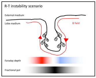
then we might plausibly observe a rapid reversal in the direction of across the tip of the finger when viewed from above, with accompanying depolarization (see Figure 17 for a schematic). Indeed, Seta et al. (2013) have already proposed that the presence of thermal plasma in the western lobe might be explained via this mechanism, so we start by assessing whether the R-T mechanism might operate, before commenting on its ability to explain our broader observations.
For the instability to go, the lobes must be at least slightly over-pressured relative to the external environment, which they may be by up to a factor of five (Seta et al., 2013, though with significant uncertainty; see Section VI.1.3). Chandrasekhar (1961) showed that the R-T instability is stabilized for all angular wavenumbers larger than , where
| (15) |
and is the acceleration of the interface, and are the mass densities of the external and lobe-based plasmas, is the magnetic field strength, and is the angle between the magnetic field and the wavevector associated with .
We do not know the acceleration of the lobe ICM-interface due to their pressure mismatch, but we can estimate the required acceleration as follows. The R-T instabilities must operate on scales at least as small as 5 kpc, which corresponds to cm-1. Rearranging Eqn. 15 to solve for , then setting g cm-3 (based on the Seta et al. 2013 estimate provided in Section VI.1.3, which is uncertain, but see below), g cm-3 (based on the assumption that the lobe contains no thermal plasma prior to the onset of the instability), , and using our previous value for , we find cm s-2. The timescale for the instability to develop is then given by (Chandrasekhar, 1961; De Young, 2003):
where all symbols have their previously defined meanings. This is the -folding time, so several times this value is the approximate timescale at which the instability becomes well-developed. Note that the result is not especially sensitive to the value of .
Thus, the lobe-ICM interface may be R-T unstable, and R-T fingers could form rapidly if this is so. However, a direct connection between R-T fingers and the observed Faraday depth structure seems unlikely for the following reasons: Given the estimated ICM density in the vicinity of the lobes, R-T fingers cannot generate the required Faraday depths over plausible path lengths without significant cooling or strong local enhancements in the local magnetic field strength (Section VI.3). In the former case, it is not clear what mechanism would lead the ICM to cool suddenly upon intrusion into the lobes. The latter possibility will have the effect of inhibiting the formation of turbulent magnetoionic sub-structure in the R-T finger, which is necessary to produce Faraday depolarization in this scenario (Stone & Gardiner, 2007a, b).
VI.5.3 Advected ISM from NGC 1316
As discussed in Section VI.4, both observations and simulations demonstrate that buoyant radio lobes are capable of lifting thermal ISM from their hosts and mixing it inhomogeneously throughout their volume. Indeed, this is our favored scenario for the origin of the thermal plasma associated with the low- patches. We now propose the following toy model (depicted in Figure 18) to account for the associated Faraday depth structure within this framework: Blobs of thermal plasma laced with G strength magnetic fields (e.g. Moss & Shukurov, 1996; Omar & Paswan, 2017) are lifted from the host galaxy ISM or surrounding ICM and entrained in vortical flows set up in the buoyant radio lobe. The plasma is dragged into shells or filaments (e.g. see Hillel & Soker, 2017; Weinberger et al., 2017), shearing and stretching the embedded magnetic field into loops. From a range of viewing angles (e.g. from positions ‘y’ and ‘z’ indicated in Figure 18), lines-of-sight intersect these shell walls/filaments tangentially over considerable path lengths, generating a substantial associated Faraday depth (see below). Across the intersecting tangent plane, we see reversals in the LOS-projected magnetic field direction, and thus the sign of the peak Faraday depth. At the same time, when viewed from a different location, the same plasma filament may produce little in the way of observable Faraday rotation or depolarization (e.g. from position ‘x’ in Figure 18). In this way, regions of the lobe exhibiting enhanced Faraday depths and depolarization will be limited to sight-lines that simultaneously contain a substantial column density of advected thermal plasma, and a substantial LOS-projected magnetic field component. These two factors will tend to be positively correlated by the vortical flow patterns, leading naturally to the generation of spatially-limited regions in which the peak Faraday depth can be substantially larger than the immediate surroundings.
To calculate the Faraday depths plausibly associated with these structures, we take Seta et al. 2013’s estimate of the electron density of thermal material in the lobe for (see Section VI.1.3), from Section VI.1.4, and the length of a typical low- patch (Section VI.1.1) as a proxy for the path length intercepted along the wall of a thermal plasma shell, and find that Faraday depths of up to 100s rad m-2 might be generated. With such high Faraday depths, mixing of the relativistic and thermal plasma, or inhomogeneities in the advected medium, will naturally produce large differential Faraday depths and dispersions, thereby accounting for the observed depolarization and the associated complexity of the frequency-dependent polarized signal.
This basic scenario has several advantages over those previously considered. Generally:
-
1.
Advected filaments/shells are naturally produced in simulations on roughly the correct timescales and length-scales (e.g. see Fig. 9 of Weinberger et al. 2017)
-
2.
Vortical flows will naturally shear the advected magnetized thermal material into structures possessing a comparatively large characteristic scale length, and thus magnetic coherence length. As a result, the required local levels of enhancement in and/or over the lobe averages (discussed in Section VI.3) are considerably relaxed.
-
3.
Presumably, there will be no special viewing angles required to observe the interfaces — a wide range of lines of sight will intersect the putative thermal plasma shells tangentially, producing the effect.
-
4.
Spatial correlations between the low- patches, , the sky-projected magnetic field, and even Stokes filaments will all arise naturally, since each observable is generated throughout the bulk of the lobe in a global flow. In particular, the position of maximum depolarization and the interfaces should be roughly coincident, since they both arise from looking along the wall/axis of a shell/filament.
Nevertheless, the true viability of this scenario is not simple to assess — it will need to be tested with simulations capable of generating high-resolution, detailed maps of Faraday depth structure in buoyant radio bubbles. At the same time, the ubiquity of these features in the radio lobe population will need to be established with broadband observations of large samples of spatially-resolved sources. Despite these caveats, we consider this basic scenario to be the most promising explanation for our observational results taken as a whole.
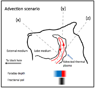
VI.6. Concluding remarks
The frequency-dependent polarization behavior associated with the low- patches in Fornax A is both pronounced and remarkable. So far as we are aware, such behavior has not been observed towards radio lobes before. This may be because as an old, large, well-resolved radio source, which is neither FR I nor FR II, and which has evolved relatively passively over an extended period on the outskirts of a poor cluster, Fornax A is itself a unique object in our skies. Alternatively, it may be that other radio lobes do show such structure, but that this has formerly gone undetected. Previous spatially-resolved studies of the Faraday effect towards radio lobes have often claimed that the observed polarization angle has a linear dependence on , and that where depolarization in is observed, it can be explained by the action of a simple turbulent magnetized plasma lying in the foreground. However, these studies generally rely on interpolating polarization behavior between a handful of narrow, widely-spaced observing bands. A great deal of subtle Faraday structure can be missed in this way — it is much like attempting to reconstruct a complex, extended object by applying aperture synthesis imaging to data from an array consisting of only a few baselines (e.g. see Brentjens & de Bruyn, 2005; Anderson, 2016b).
Indeed, it would be surprising if this latter alternative were not the case for well-evolved radio lobes. A large body of 2D, 2.5D (i.e. axisymmetric) and 3D hydrodynamic, magnetohydrodynamic, and relativistic magnetohydrodynamic simulations of the evolution and impact of radio lobes in various cosmic environments now exists (e.g. Bicknell et al., 1990; Brüggen & Kaiser, 2001; Krause & Alexander, 2007; Huarte-Espinosa et al., 2011; Hardcastle & Krause, 2014; English et al., 2016; Yang & Reynolds, 2016; Hillel & Soker, 2017; Weinberger et al., 2017, and refs. in each). These generally show that in the later stages of their evolution, radio lobes are subject to bulk vortical motions and surface instabilities, which generally reorganize and amplify frozen-in magnetic field lines, and which can advect and mix with thermal plasma from the environment. The final magneto-ionic structure of the radio lobes is generally complicated, and we can reasonably expect that complicated frequency-dependent interference effects in the polarized signal from these regions will be the norm. Perhaps these signatures have previously been masked by Faraday rotation in the deep cluster potentials that observations have typically focused on, or by some combination of poor frequency coverage and sampling, insufficient spatial resolution, intrinsic Faraday depolarization in the observing band, or insufficient accuracy attainable in polarization calibration — these are all issues of practical importance, but separate to that of whether or not the polarization signatures are generated by the lobes in the first place. Thus, it may be that re-observing large and powerful radio sources over broad, densely-sampled bands could yield new observational insights into the physics of radio lobes. We are engaged in several current (e.g. Kaczmarek et al., 2018) and planned projects to do just this.
To our knowledge, existing simulations lack the volumetric resolution to predict the spectropolarimetric signatures of realistic structures generated by instabilities at the lobe-external medium interface, and perhaps the material found deeper inside. Future work along these lines will be immensely valuable for comparison against broadband observations, which may provide a powerful new capability for tracing magnetic field structure and flow patterns in radio lobes.
VII. Summary and conclusions
We have examined the radio polarization properties of Fornax A over 1.28–3.1 GHz using RM synthesis and (,)-fitting. In this work (the first of two associated papers), our primary goal was to constrain the physical origin of the prominent low- patches in the lobes. Our principal findings are that:
-
i)
The low- patches are in general spatially-resolved, centered around enhancements in the value of of typically up to 50 rad m-2 (sometimes greater), and around ‘interfaces’ across which the Faraday depth often changes sign and jumps by – rad m-2. We argued that this implies the operation of a physical process that spatially couples depolarized Faraday structures to changes in the regular line of sight magnetic field.
-
ii)
Strong and often oscillatory (as a function of ) depolarization is observed in and around the low- patches. Thus, the polarized emission is not consistent with having experienced pure Faraday rotation by a magnetized foreground plasma, nor frequency-independent depolarization. Our (,) fitting analysis generally requires various combinations of multiple emission components, with both internal and external Faraday depolarization acting upon them, to describe the net spectropolarimetric behavior along most sight-lines. Thus, the magnetoionic structure of the Faraday-active medium is highly complicated.
-
iii)
The low- patches sit near regions where the sky-projected magnetic field orientation possesses turbulent, small-scale structure relative to other locations in the lobe. There are also indications of a relationship between the position of low- patches and that of bright Stokes filaments, but the nature of this relationship is less clear-cut. The fact that fractional polarization in the former regions is frequency-dependent, and analysis of the gradient in the sky-projected magnetic field orientation, rules out ‘crossed’ magnetic field lines in such regions as the direct cause of the low polarization values. Instead, the low- patches and Faraday depth interfaces appear to trace junctures in the magnetic field structure of the lobes, and by extension, bulk flows in the lobe medium.
-
iv)
We have considered several possible causes of the low- patches and the associated Faraday depth structure. We rule out, or otherwise disfavor, scenarios involving material transported into the lobes by the radio jet or external transiting galaxies, foreground material such as filaments in the ICM, and Rayleigh-Taylor or Kelvin-Helmholtz instabilities acting at the lobe-ICM surface.
-
v)
We find that the low- patches and associated Faraday depth enhancements are associated with a minimum of of magnetized thermal plasma residing in the lobes, most likely advected from the host galaxy ISM through buoyant uplift. We have proposed a toy model that links this material to the low- patches, to the observed enhancements in peak Faraday depth, and to the sign-reversals in peak Faraday depth that occur in these locations. In short: Vortical motion in the rising lobes shear the uplifted thermal plasma into shells or filaments, with frozen-in magnetic fields being sheared into elongated loops within. Lines-of-sight intersect these shell walls/filaments tangentially over considerable path lengths, producing associated Faraday depths of perhaps up to 100s rad m-2. The LOS-projected magnetic field reverses across the tangent plane, generating the sign reversals in peak Faraday depth. Inhomogeneities in the magnetoionic structure of this thermal material, or a co-located suffusion of synchrotron-emitting plasma, result in large Faraday dispersions and/or differential Faraday depths, generating the associated depolarization.
-
vi)
To our knowledge, and regardless of its cause, such pronounced complex frequency-dependent spectropolarimetric behavior has not yet been observed in other lobed objects. This may be because Fornax A is somewhat unique in terms of its object type, age, environment, size, or brightness, but it may also be due to previous observations lacking dense and broad coverage. Re-observation of previously-observed ‘classic’ radio galaxies using broad, densely-sampled observing bands may uncover similar structures.
-
vii)
Broadband polarimetry may provide a unique and powerful new means of tracing and characterizing flow structures in radio lobes and mixing at the lobe-ICM interface. Such observations would be particularly useful for comparison with modern simulations of radio lobes in various environments.
In paper 2, we will present further analysis of the spectral behavior of the Fornax A lobes, over their full area, in both total intensity and linear polarization. We are also currently pursuing broadband polarimetric observations of a larger sample of lobed radio sources located in different environments to further explore the scenarios described in this work.
VIII. Acknowledgements
We are indebted to the referee Jean Eilek for providing constructive feedback and criticisms of our work — several key aspects of our discussion and conclusions have changed significantly as a result. B. M. G. and C. S. A. acknowledge the support of the Australian Research Council (ARC) through grant FL100100114. B. M. G. acknowledges the support of the Natural Sciences and Engineering Research Council of Canada (NSERC) through grant RGPIN-2015-05948, and of the Canada Research Chairs program. The Dunlap Institute is funded through an endowment established by the David Dunlap family and the University of Toronto. The Australia Telescope Compact Array is part of the Australia Telescope National Facility which is funded by the Commonwealth of Australia for operation as a National Facility managed by CSIRO.
References
- Ackermann et al. (2016) Ackermann, M., Ajello, M., Baldini, L., et al. 2016, ApJ, 826, 1
- Akaike (1974) Akaike, H. 1974, IEEE Transactions on Automatic Control, 19, 716
- Alexander (2002) Alexander, P. 2002, MNRAS, 335, 610
- Anderson (2016b) Anderson, C. 2016b, PhD thesis, The University of Sydney, http://hdl.handle.net/2123/16014
- Anderson et al. (2016) Anderson, C. S., Gaensler, B. M., & Feain, I. J. 2016, ApJ, 825, 59
- Anderson et al. (2015) Anderson, C. S., Gaensler, B. M., Feain, I. J., & Franzen, T. M. O. 2015, ApJ, 815, 49
- Beletsky et al. (2011) Beletsky, Y., Gadotti, D. A., Moiseev, A., Alves, J., & Kniazev, A. 2011, MNRAS, 418, L6
- Bicknell et al. (1990) Bicknell, G. V., Cameron, R. A., & Gingold, R. A. 1990, ApJ, 357, 373
- Bland-Hawthorn et al. (1995) Bland-Hawthorn, J., Ekers, R. D., van Breugel, W., Koekemoer, A., & Taylor, K. 1995, ApJ, 447, L77
- Brentjens & de Bruyn (2005) Brentjens, M. A., & de Bruyn, A. G. 2005, A&A, 441, 1217
- Briggs (1995) Briggs, D. S. 1995, in Bulletin of the American Astronomical Society, Vol. 27, American Astronomical Society Meeting Abstracts, 1444
- Brüggen & Kaiser (2001) Brüggen, M., & Kaiser, C. R. 2001, MNRAS, 325, 676
- Brüggen & Kaiser (2002) —. 2002, Nature, 418, 301
- Burn (1966) Burn, B. J. 1966, MNRAS, 133, 67
- Cabral & Leedom (1993) Cabral, B., & Leedom, L. C. 1993, in Proceedings of the 20th annual conference on Computer graphics and interactive techniques (2 Penn Plaza, Suite 701, New York, NY: ACM), 263–270
- Cantiello et al. (2013) Cantiello, M., Grado, A., Blakeslee, J. P., et al. 2013, A&A, 552, A106
- Carilli et al. (1988) Carilli, C. L., Perley, R. A., & Dreher, J. H. 1988, ApJ, 334, L73
- Chandrasekhar (1961) Chandrasekhar, S. 1961, Hydrodynamic and Hydromagnetic Stability (Oxford University Press)
- Churazov et al. (2001) Churazov, E., Brüggen, M., Kaiser, C. R., Böhringer, H., & Forman, W. 2001, ApJ, 554, 261
- Clarke et al. (1992) Clarke, D. A., Bridle, A. H., Burns, J. O., Perley, R. A., & Norman, M. L. 1992, ApJ, 385, 173
- de Gouveia dal Pino & Opher (1989) de Gouveia dal Pino, E. M., & Opher, R. 1989, ApJ, 342, 686
- De Young (2003) De Young, D. S. 2003, MNRAS, 343, 719
- Dong & Stone (2009) Dong, R., & Stone, J. M. 2009, ApJ, 704, 1309
- Dreher et al. (1987) Dreher, J. W., Carilli, C. L., & Perley, R. A. 1987, ApJ, 316, 611
- Drinkwater et al. (2001) Drinkwater, M. J., Gregg, M. D., & Colless, M. 2001, ApJ, 548, L139
- Dursi & Pfrommer (2008) Dursi, L. J., & Pfrommer, C. 2008, ApJ, 677, 993
- Dvorkin & Rephaeli (2015) Dvorkin, I., & Rephaeli, Y. 2015, MNRAS, 450, 896
- Ekers et al. (1983) Ekers, R. D., Goss, W. M., Wellington, K. J., et al. 1983, A&A, 127, 361
- Ekers & Rots (1979) Ekers, R. D., & Rots, A. H. 1979, in Astrophysics and Space Science Library, Vol. 76, IAU Colloq. 49: Image Formation from Coherence Functions in Astronomy, ed. C. van Schooneveld (Netherlands: Springer), 61
- English et al. (2016) English, W., Hardcastle, M. J., & Krause, M. G. H. 2016, MNRAS, 461, 2025
- Feldmeier et al. (2007) Feldmeier, J. J., Jacoby, G. H., & Phillips, M. M. 2007, ApJ, 657, 76
- Fomalont et al. (1989) Fomalont, E. B., Ebneter, K. A., van Breugel, W. J. M., & Ekers, R. D. 1989, ApJ, 346, L17
- Foreman-Mackey et al. (2013) Foreman-Mackey, D., Hogg, D. W., Lang, D., & Goodman, J. 2013, PASP, 125, 306
- Forman et al. (1985) Forman, W., Jones, C., & Tucker, W. 1985, ApJ, 293, 102
- Frank et al. (1996) Frank, A., Jones, T. W., Ryu, D., & Gaalaas, J. B. 1996, ApJ, 460, 777
- Gardner & Whiteoak (1966) Gardner, F. F., & Whiteoak, J. B. 1966, ARA&A, 4, 245
- Gardner & Whiteoak (1971) —. 1971, Australian Journal of Physics, 24, 899
- Geldzahler & Fomalont (1984) Geldzahler, B. J., & Fomalont, E. B. 1984, AJ, 89, 1650
- Green (2011) Green, D. A. 2011, Bulletin of the Astronomical Society of India, 39, 289
- Guidetti et al. (2011) Guidetti, D., Laing, R. A., Bridle, A. H., Parma, P., & Gregorini, L. 2011, MNRAS, 413, 2525
- Guidetti et al. (2012) Guidetti, D., Laing, R. A., Croston, J. H., Bridle, A. H., & Parma, P. 2012, MNRAS, 423, 1335
- Hales et al. (2012) Hales, C. A., Gaensler, B. M., Norris, R. P., & Middelberg, E. 2012, MNRAS, 424, 2160
- Hardcastle (2010) Hardcastle, M. J. 2010, MNRAS, 405, 2810
- Hardcastle & Krause (2014) Hardcastle, M. J., & Krause, M. G. H. 2014, MNRAS, 443, 1482
- Heald et al. (2009) Heald, G., Braun, R., & Edmonds, R. 2009, A&A, 503, 409
- Heiles & Haverkorn (2012) Heiles, C., & Haverkorn, M. 2012, Space Sci. Rev., 166, 293
- Hillel & Soker (2017) Hillel, S., & Soker, N. 2017, ApJ, 845, 91
- Horellou et al. (2001) Horellou, C., Black, J. H., van Gorkom, J. H., et al. 2001, A&A, 376, 837
- Huarte-Espinosa et al. (2011) Huarte-Espinosa, M., Krause, M., & Alexander, P. 2011, MNRAS, 417, 382
- Iodice et al. (2017) Iodice, E., Spavone, M., Capaccioli, M., et al. 2017, ApJ, 839, 21
- Iyomoto et al. (1998) Iyomoto, N., Makishima, K., Tashiro, M., et al. 1998, ApJ, 503, L31
- Jones et al. (1997) Jones, C., Stern, C., Forman, W., et al. 1997, ApJ, 482, 143
- Kaczmarek et al. (2018) Kaczmarek, J. F., Purcell, C. R., Gaensler, B. M., et al. 2018, MNRAS, doi:10.1093/mnras/sty269
- Kaiser et al. (2005) Kaiser, C. R., Pavlovski, G., Pope, E. C. D., & Fangohr, H. 2005, MNRAS, 359, 493
- Kaneda et al. (1995) Kaneda, H., Tashiro, M., Ikebe, Y., et al. 1995, ApJ, 453, L13
- Karimabadi et al. (2013) Karimabadi, H., Roytershteyn, V., Wan, M., et al. 2013, Physics of Plasmas, 20, 012303
- Kim & Fabbiano (2003) Kim, D.-W., & Fabbiano, G. 2003, ApJ, 586, 826
- Kim et al. (1998a) Kim, D. W., Fabbiano, G., & Mackie, G. 1998a, ApJ, 497, 699
- Kim et al. (1998b) —. 1998b, ApJ, 497, 699
- Kirkpatrick et al. (2009) Kirkpatrick, C. C., McNamara, B. R., Rafferty, D. A., et al. 2009, ApJ, 697, 867
- Krause & Alexander (2007) Krause, M., & Alexander, P. 2007, MNRAS, 376, 465
- Laing (1980) Laing, R. A. 1980, MNRAS, 193, 439
- Laing & Bridle (2002) Laing, R. A., & Bridle, A. H. 2002, MNRAS, 336, 1161
- Laing et al. (2008) Laing, R. A., Bridle, A. H., Parma, P., & Murgia, M. 2008, MNRAS, 391, 521
- Lanz et al. (2010) Lanz, L., Jones, C., Forman, W. R., et al. 2010, ApJ, 721, 1702
- Ma et al. (2014) Ma, X., Otto, A., & Delamere, P. A. 2014, Journal of Geophysical Research: Space Physics, 119, 781
- Machacek et al. (2005) Machacek, M., Dosaj, A., Forman, W., et al. 2005, ApJ, 621, 663
- Mackie & Fabbiano (1998) Mackie, G., & Fabbiano, G. 1998, AJ, 115, 514
- Mason et al. (1988) Mason, A., Morrison, P., & Sadun, A. C. 1988, Nature, 333, 640
- McKinley et al. (2015) McKinley, B., Yang, R., López-Caniego, M., et al. 2015, MNRAS, 446, 3478
- McNamara & Nulsen (2007) McNamara, B. R., & Nulsen, P. E. J. 2007, ARA&A, 45, 117
- McNamara & Nulsen (2012) —. 2012, New Journal of Physics, 14, 055023
- Moss & Shukurov (1996) Moss, D., & Shukurov, A. 1996, MNRAS, 279, 229
- Norman & Balsara (1993) Norman, M. L., & Balsara, D. S. 1993, in Lecture Notes in Physics, Berlin Springer Verlag, Vol. 421, Jets in Extragalactic Radio Sources, ed. H.-J. Röser & K. Meisenheimer, 229
- Obergaulinger et al. (2010) Obergaulinger, M., Aloy, M. A., & Müller, E. 2010, A&A, 515, A30
- Offringa et al. (2010) Offringa, A. R., de Bruyn, A. G., Biehl, M., et al. 2010, MNRAS, 405, 155
- Omar & Paswan (2017) Omar, A., & Paswan, A. 2017, ArXiv e-prints, arXiv:1705.00805
- O’Sullivan et al. (2017) O’Sullivan, S. P., Purcell, C. R., Anderson, C. S., et al. 2017, ArXiv e-prints, arXiv:1705.00102
- O’Sullivan et al. (2013) O’Sullivan, S. P., Feain, I. J., McClure-Griffiths, N. M., et al. 2013, ApJ, 764, 162
- Owen et al. (1990) Owen, F. N., Eilek, J. A., & Keel, W. C. 1990, ApJ, 362, 449
- Paolillo et al. (2002) Paolillo, M., Fabbiano, G., Peres, G., & Kim, D.-W. 2002, ApJ, 565, 883
- Pavlovski et al. (2007) Pavlovski, G., Kaiser, C. R., & Pope, E. C. D. 2007, ArXiv e-prints, arXiv:0709.1796
- Perley et al. (1984) Perley, R. A., Bridle, A. H., & Willis, A. G. 1984, ApJS, 54, 291
- Pizzolato & Soker (2006) Pizzolato, F., & Soker, N. 2006, MNRAS, 371, 1835
- Pope et al. (2010) Pope, E. C. D., Babul, A., Pavlovski, G., Bower, R. G., & Dotter, A. 2010, MNRAS, 406, 2023
- Reynolds et al. (2002) Reynolds, C. S., Heinz, S., & Begelman, M. C. 2002, MNRAS, 332, 271
- Reynolds et al. (2005) Reynolds, C. S., McKernan, B., Fabian, A. C., Stone, J. M., & Vernaleo, J. C. 2005, MNRAS, 357, 242
- Roediger et al. (2013) Roediger, E., Kraft, R. P., Nulsen, P., et al. 2013, MNRAS, 436, 1721
- Russell et al. (2017) Russell, H. R., McDonald, M., McNamara, B. R., et al. 2017, ApJ, 836, 130
- Ruszkowski et al. (2007) Ruszkowski, M., Enßlin, T. A., Brüggen, M., Heinz, S., & Pfrommer, C. 2007, MNRAS, 378, 662
- Salomé et al. (2011) Salomé, P., Combes, F., Revaz, Y., et al. 2011, A&A, 531, A85
- Scharf et al. (2005) Scharf, C. A., Zurek, D. R., & Bureau, M. 2005, ApJ, 633, 154
- Schnitzeler et al. (2011) Schnitzeler, D., Banfield, J., Emonts, B., et al. 2011, Australia Telescope Technical memo # AT/39.9/129, Tech. rep., CSIRO
- Schnitzeler et al. (2015) Schnitzeler, D. H. F. M., Banfield, J. K., & Lee, K. J. 2015, MNRAS, 450, 3579
- Schulman & Fomalont (1992) Schulman, E., & Fomalont, E. B. 1992, AJ, 103, 1138
- Schweizer (1980) Schweizer, F. 1980, ApJ, 237, 303
- Seta et al. (2013) Seta, H., Tashiro, M. S., & Inoue, S. 2013, PASJ, 65, 106
- Simionescu et al. (2009) Simionescu, A., Werner, N., Böhringer, H., et al. 2009, A&A, 493, 409
- Simon & Axford (1967) Simon, M., & Axford, W. I. 1967, ApJ, 150, 105
- Sokoloff et al. (1998) Sokoloff, D. D., Bykov, A. A., Shukurov, A., et al. 1998, MNRAS, 299, 189
- Stawarz et al. (2013) Stawarz, Ł., Tanaka, Y. T., Madejski, G., et al. 2013, ApJ, 766, 48
- Sternberg & Soker (2008) Sternberg, A., & Soker, N. 2008, MNRAS, 389, L13
- Stone & Gardiner (2007a) Stone, J. M., & Gardiner, T. 2007a, Physics of Fluids, 19, 094104
- Stone & Gardiner (2007b) —. 2007b, ApJ, 671, 1726
- Stritzinger et al. (2010) Stritzinger, M., Burns, C. R., Phillips, M. M., et al. 2010, AJ, 140, 2036
- Sun et al. (2015) Sun, X. H., Rudnick, L., Akahori, T., et al. 2015, AJ, 149, 60
- Tashiro et al. (2009) Tashiro, M. S., Isobe, N., Seta, H., Matsuta, K., & Yaji, Y. 2009, PASJ, 61, S327
- Turner & Shabala (2015) Turner, R. J., & Shabala, S. S. 2015, ApJ, 806, 59
- van Breugel & Fomalont (1984) van Breugel, W., & Fomalont, E. B. 1984, ApJ, 282, L55
- Venturi & Taylor (1999) Venturi, T., & Taylor, G. B. 1999, AJ, 118, 1931
- Weinberger et al. (2017) Weinberger, R., Ehlert, K., Pfrommer, C., Pakmor, R., & Springel, V. 2017, MNRAS, 470, 4530
- Werner et al. (2011) Werner, N., Sun, M., Bagchi, J., et al. 2011, MNRAS, 415, 3369
- Wilson (1989) Wilson, M. J. 1989, in Lecture Notes in Physics, Berlin Springer Verlag, Vol. 327, Hot Spots in Extragalactic Radio Sources, ed. K. Meisenheimer & H.-J. Roeser, 215–218
- Wilson et al. (2011) Wilson, W. E., Ferris, R. H., Axtens, P., et al. 2011, MNRAS, 416, 832
- Yang & Reynolds (2016) Yang, H.-Y. K., & Reynolds, C. S. 2016, ApJ, 829, 90
Appendix A Ancillary images