One-proton emission from the ${}^{6}_{\Lambda}$Li hypernucleus

Abstract

One-proton (1p) radioactive emission under the influence of the $\Lambda^{0}$-hyperon inclusion is discussed. I investigate the hyper-1p emitter, ${}^{6}_{\Lambda}$Li, with a time-dependent three-body model. Two-body interactions for $\alpha$-proton and $\alpha$-$\Lambda^{0}$ subsystems are determined consistently to their resonant and bound energies, respectively. For a proton-$\Lambda^{0}$ subsystem, a contact interaction, which can be linked to the vacuum-scattering length of the proton-$\Lambda^{0}$ scattering, is employed. A noticeable sensitivity of the 1p-emission observables to the scattering length of the proton-$\Lambda^{0}$ interaction is shown. The $\Lambda^{0}$-hyperon inclusion leads to a remarkable fall of the 1p-resonance energy and width from the hyperon-less $\alpha$-proton resonance. For some empirical values of the proton-$\Lambda^{0}$ scattering length, the 1p-resonance width is suggested to be of the order of $0.1-0.01$ MeV. Thus, the 1p emission from ${}^{6}_{\Lambda}$Li may occur in the timescale of $10^{-20}-10^{-21}$ seconds, which is sufficiently shorter than the self-decay lifetime of $\Lambda^{0}$, $10^{-10}$ seconds. By taking the spin-dependence of the proton-$\Lambda^{0}$ interaction into account, a remarkable split of the $J^{\pi}=1^{-}$ and $2^{-}$ 1p-resonance states is predicted. It is also suggested that, if the spin-singlet proton-$\Lambda^{0}$ interaction is sufficiently attractive, the 1p emission from the $1^{-}$ ground state is forbidden. From these results, I conclude that the 1p emission can be a suitable phenomenon to investigate the basic properties of the hypernuclear interaction, for which a direct measurement is still difficult.

I Introduction

Inclusion of hyperons in atomic nuclei has been a fascinating topic in nuclear physics Gal et al. (2016); Feliciello and Nagae (2015); Botta et al. (2012). One of the famous effects is that the hyperon plays as a gluelike particle: its inclusion leads to an expansion of the proton and neutron driplines, as well as a new emergence of stable nuclei. Recently, one novel type of the hypernuclear experiment combined with the heavy-ion collision has been proposed Rappold (2016); Steinheimer et al. (2012); Asai et al. (1984); Baltz et al. (1994). An advantage of this new experimental method is an accessibility to the proton-rich and neutron-rich regions, where the inclusion effect can provide a noticeable difference from the normal nuclei.

The fundamental parts of the hypernuclear physics include hyperon-nucleon (YN) and hyperon-hyperon (YY) interactions. However, even with the modern experimental development, a direct measurement of the YN and/or YY interactions is still difficult. This lack of information has been indeed a long-standing bottleneck to establish the unified nuclear model for normal and hyper nuclei.

On the other hand, in recent decades, there has been a remarkable development of experiments to measure the few-nucleon radioactive emissions. Those include, e.g. one-proton (1p) and two-proton emissions 02Pfu ; 02Gio ; Pfützner et al. (2012); Grigorenko (2009). For these radioactive processes, typical observable quantities include the few-nucleon resonance energy and its decay width or equivalently lifetime. Here it is worth mentioning that the decay width is available only in these meta-stable systems, in contrast to the bound systems, whose lifetime is trivially infinite. It has been expected that these observables can be good reference quantities for the theoretical models of the nuclear force, pairing correlation, and multi-particle dynamics. Similarly, the particle-unbound hyper nuclei can be a good testing field to investigate the hypernuclear properties. There have been, however, still less studies of the hyperon-inclusion effect on the particle-unbound systems Motoba et al. (1983); Hiyama et al. (1996); Belyaev et al. (2008); Hiyama and Yamada (2009); 2015Hiyama .

The aim of this work is to invoke the interest to utilize the proton emission as a suitable tool to investigate the hypernuclear properties. For this purpose, I demonstrate a simple calculation for the lightest hyper-1p emitter, ${}^{6}_{\Lambda}$Li. The calculation is based on the $\alpha$-proton-$\Lambda^{0}$ three-body model to study the inclusion effect of $\Lambda^{0}$ hyperon on the proton-emitting nucleus. For the description of the particle-resonance, or equivalently, the meta-stable properties, it is necessary to extend the static quantum mechanics. The popular methods for this purpose include the time-dependent method 04Gurv ; Oishi et al. (2014, 2017); Ordonez and Hatano (2017), as well as the non-Hermitian method Ho (1983); Michel et al. (2002); Myo et al. (2014); 2015Hiyama . In this paper, I employ the former option, which can provide one phenomenological way to find a useful link between the resonance observables and the basic properties in hypernuclear physics. Especially, it is expected that the measurement of the proton emission provides suitable data to examine the YN interaction model. Note that the similar interest has been devoted to the two-proton radioactive emission, where its decay width can be closely related to the proton-proton scattering length Grigorenko et al. (2000); Oishi et al. (2017).

In the next section, the formalism of the three-body model is presented. Parameters of the model are chosen consistently with the experimental data. In section III, the time-dependent calculation for the hyper-1p emitter, ${}^{6}_{\Lambda}$Li, is presented. There, my result and discussion on the hyperon-inclusion effect on the 1p emission are described in detail. Finally, in section IV, I summarize this work.

II Three-body Model

For simplicity, I omit the superscript $0$ for the $\Lambda^{0}$ particle in the following. The theoretical model is based on the $\alpha$-proton-$\Lambda$ three-body picture, within the core-orbital coordinates, $\left\{\bm{r}_{\rm p},\bm{r}_{\Lambda}\right\}$, as shown in Fig. 1. The detailed formalism of these coordinates is summarized in the Appendix. In this framework, the total Hamiltonian reads Bertsch and Esbensen (1991); Esbensen et al. (1997); Hagino and Sagawa (2005)

$$H_{3b} = h_{\rm p}+h_{\Lambda}+x_{\rm rec}+v_{\rm p-\Lambda}(\bm{r}_{\rm p},\bm{r}_{\Lambda}),$$

$$h_{i} = \frac{p_{i}^{2}}{2\mu_{i}}+V_{\alpha-i}(r_{i}),$$

$$x_{\rm rec} = \frac{\bm{p}_{\rm p}\cdot\bm{p}_{\Lambda}}{m_{\rm c}}~{}~{}~{}({\rm recoil~{}term}),$$ (1)

where $i={\rm p}$ and $\Lambda$ for the valence proton and $\Lambda$ hyperon, respectively. Here $\bm{r}_{i}$ is the relative coordinate between the core and the $i$-th nucleon. Thus, $h_{i}$ is the corresponding single particle (s.p.) Hamiltonian. Mass parameters are fixed as the empirical values: $\mu_{i}=m_{i}m_{\rm c}/(m_{i}+m_{\rm c})$, $m_{\rm p}=938.272$ MeV$/c^{2}$, $m_{\Lambda}=1115.683$ MeV$/c^{2}$, and $m_{\rm c}=3727.379$ MeV$/c^{2}$ ($\alpha$-particle mass).

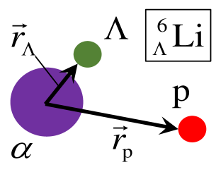
FIG. 1: Three-body model of ${}^{6}_{\Lambda}$Li.

TABLE 1: Resonance energy and width obtained with the $\alpha$-nucleon potential in this work. Those are evaluated from the scattering phase-shift in the $(p_{3/2})$-channel.

		$E_{\rm\alpha-n},~{}\Gamma_{\rm\alpha-n}$	$E_{\rm\alpha-p},~{}\Gamma_{\rm\alpha-p}$
		(MeV)	(MeV)
Our $V_{\rm\alpha-n,p}$		$0.77,~{}0.67$	$1.69,~{}1.31$
Exp.02Till		$0.798,~{}0.578$	$1.69,~{}1.06$
Exp.88Ajzen		$0.89,~{}0.60$	$1.97,~{}(\simeq 1.5)$
Exp.NNDCHP		$0.735,~{}0.60$	$1.96(5),~{}(\simeq 1.5)$

The core-proton potential is determined as

$$V_{\rm\alpha-p}(\bm{r}_{\rm p})=V_{WS}(\bm{r}_{\rm p})+V_{Coul}(\bm{r}_{\rm p}),$$ (2)

where a Woods-Saxon potential including the spin-orbit term is given as

$$V_{WS}(r) = V_{0}f(r)+U_{ls}(\bm{l}\cdot\bm{s})\frac{1}{r}\frac{df(r)}{dr},$$ (3)

$$f(r) = \frac{1}{1+e^{(r-R_{0})/a_{0}}}.$$ (4)

Here $r=\left|\bm{r}\right|$ and $f(r)$ is a standard Fermi profile. In addition, Coulomb potential of an uniformly charged sphere with its radius $R_{0}$ is included for this subsystem. In this paper, its parameters are fixed as $R_{0}=r_{0}\cdot 4^{1/3}$, $r_{0}=1.25$ fm, $a_{0}=0.65$ fm, $V_{0}=-47.4$ MeV, and $U_{ls}=-0.4092V_{0}r_{0}^{2}$ Esbensen et al. (1997); Hagino and Sagawa (2005). From the phase-shift analysis, it is confirmed that this set of parameters fairly reproduces the empirical $\alpha$-neutron and $\alpha$-proton scattering data in the $p_{3/2}$ channel 02Till , as summarized in TABLE 1. On the other hand, the core-$\Lambda$ potential is given as

$$V_{\alpha-\Lambda}(\bm{r}_{\Lambda})=fV_{WS}(r_{\Lambda}),$$ (5)

with the reduction factor, $f=0.5333$, where the non-physically large spin-orbit component in Eq. (3) is not operative. This potential correctly reproduces the s.p. binding energy in the core-$\Lambda$ subsystem (${}^{5}_{\Lambda}$He) in the $s_{1/2}$ channel, $\epsilon(s_{1/2})=-3.12$ MeV Gal (1975).

II.1 Proton-$\Lambda$ interaction

In this work, for the proton-$\Lambda$ subsystem, I employ the simple contact-type interaction:

$$v_{\rm p-\Lambda}(\bm{r}_{\rm p},\bm{r}_{\Lambda})=w_{0}\delta(\bm{r}_{\rm p}-\bm{r}_{\Lambda}).$$ (6)

As is well known, its bare strength, $w_{0}$, can be determined consistently to the vacuum proton-$\Lambda$ scattering length, $a_{v}$, by determining also the energy cutoff $E_{\rm cut}$ of the model space Bertsch and Esbensen (1991); Esbensen et al. (1997). That is,

$$a_{v}=\left[\frac{2k_{\rm cut}}{\pi}+\frac{2\pi\hbar^{2}}{\mu_{\rm p-\Lambda}w_{0}}\right]^{-1}~{}~{}({\rm fm}),$$ (7)

or equivalently,

$$w_{0}=\frac{2\pi^{2}\hbar^{2}a_{v}}{\mu_{\rm p-\Lambda}(\pi-2a_{v}k_{\rm cut})}~{}~{}~{}~{}({\rm MeVfm^{3}}),$$ (8)

where $\mu_{\rm p-\Lambda}=m_{\rm p}m_{\Lambda}/(m_{\rm p}+m_{\Lambda})$ and $k_{\rm cut}=\sqrt{2\mu_{\rm p-\Lambda}E_{\rm cut}}/\hbar$. The energy cutoff is fixed as $E_{\rm cut}=15$ MeV in this paper. Unfortunately, there has been no direct measurement available for the $\Lambda-p$ scattering length in vacuum. Thus, in the following discussion, I treat it as a model parameter, and results with several $a_{v}$ values are compared. Also, in Sec. III.3, the model is extended to take the spin-dependence of the scattering length into account.

Note that there are several, more realistic YN-interaction models than the contact type Gal et al. (2016); Feliciello and Nagae (2015). However, these interactions have finite ranges. At present, the time-dependent calculation combined with the finite-range proton-$\Lambda$ force is not feasible, due to the numerical cost. The main problem is that, for $J^{\pi}=1^{-}$ or $2^{-}$, one needs a larger model space than in the case of $J^{\pi}=0^{+}$ Oishi et al. (2014, 2017). To employ these finite-range forces, the algorithmic improvement as well as the parallelized computation is in progress now.

II.2 Uncorrelated basis

In this work, I assume that the $\alpha$ core keeps the spin-parity of $0^{+}$ without excitation. Then, the proton-$\Lambda$ state is expanded on the uncorrelated basis, which is the tensor product of two s.p. states coupled to $J^{\pi}$. That is,

$$\ket{\Phi^{({\rm p\Lambda},J^{\pi})}_{\kappa\lambda}}=\left[\ket{\phi^{\rm(p)}_{\kappa}}\otimes\ket{\phi^{(\Lambda)}_{\lambda}}\right]^{(J^{\pi})},$$ (9)

where $\kappa$ is the shorthanded label for all the quantum numbers of the proton state, $\left\{n_{p},l_{p},j_{p},m_{p}\right\}$, and similarly with $\lambda$ for the $\Lambda$ state. Those include the radial quantum number $n$, the orbital angular momentum $l$, the spin-coupled angular momentum $j$, and the magnetic quantum number $m$. Of course, each s.p. state satisfies,

$$h_{\rm p}\ket{\phi^{\rm(p)}_{\kappa}}=\epsilon_{\kappa}\ket{\phi^{\rm(p)}_{\kappa}},~{}~{}~{}h_{\Lambda}\ket{\phi^{(\Lambda)}_{\lambda}}=\epsilon_{\lambda}\ket{\phi^{(\Lambda)}_{\lambda}},$$ (10)

where $\epsilon_{\kappa(\lambda)}$ is the single-proton ($\Lambda$) energy. In order to take into account the Pauli principle for the valence proton, the first $(s_{1/2})$ state is excluded. The s.p. angular momenta up to the $l_{\rm cut}=3$ are taken into account. The continuum s.p. states up to $E_{\rm cut}=15$ MeV are discretized in the radial box of $R_{\rm box}=120$ fm. This truncation of model space is confirmed to be in a range that ensures the convergence in the 1p-resonance observables.

The three-body eigenstates are solved by diagonalizing the Hamiltonian matrix. That is,

$$\Psi_{N}(\bm{r}_{\rm p},\bm{r}_{\Lambda})=\sum_{M}U_{NM}\Phi^{({\rm p\Lambda},J^{\pi})}_{M}(\bm{r}_{\rm p},\bm{r}_{\Lambda}),$$ (11)

where $H_{3b}\ket{\Psi_{N}}=E_{N}\ket{\Psi_{N}}$ with the expansion coefficients, $\{U_{M}\}$. Here $M=\{\kappa,\lambda\}$ is the simplified label for the uncorrelated basis.

In the following, I limit my discussion to only with the $J^{\pi}=1^{-}$ and $2^{-}$ configurations. Thus, the dominant channel is trivially $\kappa(p_{3/2})\otimes\lambda(s_{1/2})$. Notice that, in this channel, the s.p. proton state is resonant, whereas the $\Lambda$ state is bound.

The expectation value of the three-body Hamiltonian gives the total separation energy with respect to the $\alpha$-proton-$\Lambda$ breakup threshold. That is,

$$B_{\rm p\Lambda}=-E_{3b}=-\Braket{\Psi}{H_{3b}}{\Psi},$$ (12)

for an arbitrary state $\ket{\Psi}$. In the next section, for the time-evolution calculation to describe the 1p emission, Eq. (12) is utilized to evaluate the mean three-body energy of the initial state, $\ket{\Psi(t=0)}$.

II.3 Experimental data

The three-body separation energy in Eq. (12) can be associated with the two-body separation energies of the subsystems. Because of the two different orders to strip the valence proton and $\Lambda$ from the $\alpha$ core, one can formulate it in the two ways. That is,

$$B_{\rm p\Lambda}(^{6}_{\Lambda}{\rm Li}) = B_{\rm\Lambda}(^{6}_{\Lambda}{\rm Li})+B_{\rm p}(^{5}{\rm Li}),~{}~{}{\rm or}$$ (13)

$$= B_{\rm p}(^{6}_{\Lambda}{\rm Li})+B_{\rm\Lambda}(^{5}_{\Lambda}{\rm He}).$$

Here $B_{\rm p}(X)$ and $B_{\Lambda}(X)$ indicate the single-proton and single-$\Lambda$ separation energies from the $X$ nuclide, respectively. Note that, if the separation energy is positive (negative), that channel is bound (unbound). Thus, if $B_{\rm p}(^{6}_{\Lambda}{\rm Li})$ is negative, the spontaneous 1p emission can take place. That is,

$$B_{\rm p}(^{6}_{\Lambda}{\rm Li})=B_{\rm\Lambda}(^{6}_{\Lambda}{\rm Li})+B_{\rm p}(^{5}{\rm Li})-B_{\rm\Lambda}(^{5}_{\Lambda}{\rm He}).$$ (14)

From the reference data Gal (1975); 1981Bertini ; 1995Noumi ; 02Till , this is estimated as $B_{\rm p}(^{6}_{\Lambda}{\rm Li})\simeq-0.6$ MeV, and thus, ${}^{6}_{\Lambda}$Li may be active for the spontaneous 1p emission from its ground state. However, it should be also noticed that a large ambiguity of the order of $0.1-1$ MeV still remains in $B_{\rm p}(^{6}_{\Lambda}{\rm Li})$. This ambiguity is from the experimental uncertainties in $B_{\rm p}(^{5}{\rm Li})$ 88Ajzen ; 02Till ; NNDCHP and $B_{\Lambda}(^{6}_{\Lambda}{\rm Li})$ 1981Bertini ; 1995Noumi ; 1967Harmsen ; Bhaduri and Nogami (1972). Concerning these uncertainties, it should be still an open question whether the 1p emission from the ground state of ${}^{6}_{\Lambda}$Li occurs or not.

According to the several experimental searches 1967Harmsen ; Goodhead and Evans (1967), the narrow resonance of proton-${}^{5}_{\Lambda}$He has not been reported. There can be two interpretations of this result. The first one is simply that ${}^{6}_{\Lambda}$Li is bound against the 1p emission. The alternative is that 1p-resonance actually exists but with a considerably large width. In the following discussion, one can find that this problem is strongly dependent on the effective proton-$\Lambda$ interaction strength.

III Result and Discussion

First I briefly mention the case, where the spontaneous 1p emission is forbidden. In the present model, $B_{\rm\Lambda}(^{5}_{\Lambda}{\rm He})=3.12$ MeV as reproduced by the $V_{\alpha-\Lambda}(\bm{r}_{\Lambda})$ consistently to the experimental data Gal (1975). Also, the $\alpha$-proton subsystem is unbound with $B_{\rm p}(^{5}{\rm Li})=-1.69$ MeV consistently to Ref. 02Till . From Eqs. (13) and (14), when the 1p emission is forbidden as $B_{\rm p}(^{6}_{\Lambda}{\rm Li})>0$, it coincides that $E_{3b}=-B_{\rm p\Lambda}<-3.12$ MeV, or equivalently that $B_{\Lambda}(^{6}_{\Lambda}{\rm Li})>4.81$ MeV. Remember that $B_{\rm p\Lambda}$ or $B_{\Lambda}(^{6}_{\Lambda}{\rm Li})$ is controlled by the interaction strength, $w_{0}$, which is linked to the proton-$\Lambda$ scattering length, $a_{v}$.

It is confirmed that, if the spontaneous 1p emission is forbidden, it requires that $a_{v}\leq-3.1~{}(-3.3)$ fm for the $J^{\pi}=1^{-}~{}(2^{-})$ configuration. In this case, the three-body ground state is completely bound, and the valence proton and $\Lambda$ mostly occupy the $(p_{3/2})$ and $(s_{1/2})$ orbits, respectively: the occupation probability is obtained as $P(p_{3/2},s_{1/2})\cong 98~{}\%$. This dominance is attributable to the bound-$(s_{1/2})$ orbit of the $\Lambda$ particle.

On the other hand, there have been several realistic YN interaction models, which predict the larger scattering length than our 1p-binding border, $-3.1$ fm. For instance, see Ref. Nemura et al. (2002) for a summary of these values. In this case, the 1p emission may happen from the ground state of ${}^{6}_{\Lambda}$Li. In the following, along this second scenario, I discuss the $\Lambda$-inclusion effect on the 1p-emission process. For this purpose, the time-dependent method is employed.

III.1 Time-dependent method

General formalism of the time-dependent method can be found in Refs. Oishi et al. (2014, 2017). Thus, in the following, I only describe the necessary contents for this work.

As discussed in the previous section, the 1p emission is expected to occur with the energy release of $Q_{\rm 1p}=-B_{\rm p}(^{6}_{\Lambda}{\rm Li})\simeq+0.6$ MeV. To evaluate the three-body energy consistently to the expected $Q_{\rm 1p}$ value, it is convenient to reformulate Eq. (13). That is,

$$Q_{\rm 1p}=-B_{\rm p}(^{6}_{\Lambda}{\rm Li})=E_{3b}+B_{\rm\Lambda}(^{5}_{\Lambda}{\rm He}),$$ (15)

where $B_{\rm\Lambda}(^{5}_{\Lambda}{\rm He})=3.12$ MeV in the present model consistently to Ref. Gal (1975). Thus, for fitting to the expected $Q_{\rm 1p}$ value, it requires that $E_{3b}=\Braket{H_{3b}}\simeq-2.5$ MeV. Note also that the $\Lambda$-binding energy of ${}^{6}_{\Lambda}$Li is given as,

$$-B_{\Lambda}(^{6}_{\Lambda}{\rm Li})=E_{3b}+B_{\rm p}(^{5}{\rm Li}),$$ (16)

where $B_{\rm p}(^{5}{\rm Li})=-1.69$ MeV 02Till . Thus, the expected $Q_{\rm 1p}$ value corresponds to that $B_{\Lambda}(^{6}_{\Lambda}{\rm Li})\simeq+4.2$ MeV.

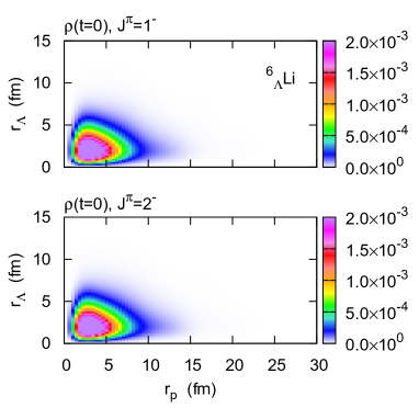
FIG. 2: Probability-density distribution at $t=0$ obtained with the confining potential procedure.

In order to fix the initial state for the time-dependent 1p emission, which should be associated with the expected $Q_{\rm 1p}$ value, I utilize the confining-potential procedure. This procedure has provided a good approximation for nuclear resonance processes Gurvitz and Kalbermann (1987); Gurvitz (1988); 04Gurv ; Maruyama et al. (2012); Oishi et al. (2014, 2017). Also, for the two-proton emitter ⁶Be Oishi et al. (2014, 2017), it has provided the consistent result with the non-Hermitian calculation of the complex-scaling method Myo et al. (2014); Jaganathen et al. (2017).

The confining potential at $t=0$ is given as

$$V_{\alpha-i}^{(c)}(\bm{r}_{i})=V_{\alpha-i}(\bm{r}_{i})+\Delta V_{\alpha-i}(\bm{r}_{i}).$$ (17)

The gap potential $\Delta V_{\alpha-i}(\bm{r}_{i})$ is determined within the same manner in Ref. Oishi et al. (2014): the wall potential at the border radius, $\left|\bm{r}_{i}\right|\geq r_{b}=5.7$ fm, is employed. Indeed, it is checked that, as long as the initial-wave packet is well confined around the $\alpha$ core, the conclusion does not change even with the different $r_{b}$ values.

Within the confining potential, the initial state can be solved by expanding it on the eigen-states of $H_{3b}$. That is,

$$\ket{\Psi(t=0)}=\sum_{N}F_{N}(0)\ket{\Psi_{N}},$$ (18)

where $H_{3b}\ket{\Psi_{N}}=E_{N}\ket{\Psi_{N}}$. Figure 2 displays the initial density of probability for the $J^{\pi}=1^{-}$ and $2^{-}$ configurations. That is,

$$\rho(r_{\rm p},r_{\Lambda})=8\pi^{2}r_{\rm p}^{2}r_{\Lambda}^{2}\int_{-1}^{1}d(\cos\theta_{\rm p\Lambda})\left|\Psi(t=0;\bm{r}_{\rm p},\bm{r}_{\Lambda})\right|^{2}.$$ (19)

Namely, the original distribution is integrated with respect to the proton-$\Lambda$ opening angle, $\theta_{\rm p\Lambda}$ Hagino and Sagawa (2005); Oishi et al. (2014). In Fig. 2, one can find that both the valence proton and $\Lambda$ are well confined around the $\alpha$ core. In this state, the $(p_{3/2},s_{1/2})$ configuration of proton and $\Lambda$ is dominant: $P(p_{3/2},s_{1/2})=97.9~{}(98.3)~{}\%$ for $J^{\pi}=1^{-}~{}(2^{-})$. This is similar to the 1p-bound state discussed already. Notice also that, due to the different orbits of the ingredient particles, the initial density has a long tail with respect to $r_{p}$, whereas it has a compact form with respect to $r_{\Lambda}$.

The three-body energy is obtained as $E_{3b}=\Braket{H_{3b}}=-2.52$ and $-2.49$ MeV for the $J^{\pi}=1^{-}$ and $2^{-}$ cases, respectively. Here the vacuum-scattering length is fixed as $a_{v}=-1.6$ fm, which corresponds to $w_{0}=-468.83~{}\rm MeVfm^{3}$, for the fitting purpose to the expected $Q_{\rm 1p}$ value.

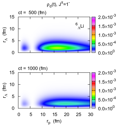
FIG. 3: Time-dependent probability-density distribution of the decay state, $\rho_{d}(t)$, for $J^{\pi}=1^{-}$.

From the initial state in Eq. (18), the time development can be solved as,

$$\ket{\Psi(t)}=\sum_{N}F_{N}(t)\ket{\Psi_{N}},$$ (20)

where $F_{N}(t)=e^{-itE_{N}/\hbar}F_{N}(0)$. It is convenient to define the decay state as,

$$\ket{\Psi_{d}(t)}\equiv\ket{\Psi(t)}-\beta(t)\ket{\Psi(0)},$$ (21)

where $\beta(t)=\Braket{\Psi(0)}{\Psi(t)}$ Bertulani et al. (2008). Since the initial state is well confined, this decay state represents the out-going component from the $\alpha$ core.

In Fig. 3, the decay-probability density for the $J^{\pi}=1^{-}$ configuration, which is normalized at each point of time, is presented. That is,

$$\rho_{d}(t;r_{\rm p},r_{\Lambda})=\frac{8\pi^{2}r_{\rm p}^{2}r_{\Lambda}^{2}}{N_{d}(t)}\int_{-1}^{1}d(\cos\theta_{\rm p\Lambda})\left|\Psi_{d}(t;\bm{r}_{\rm p},\bm{r}_{\Lambda})\right|^{2},$$ (22)

where $N_{d}(t)=\Braket{\Psi_{d}(t)}{\Psi_{d}(t)}$. In Fig. 3, one can clearly see the evacuation of the proton: the decay probability grows at $r_{p}\geq 9$ fm during the time evolution. Also, the decay probability is zero for $r_{\Lambda}\geq 6$ fm, indicating that the $\Lambda$ particle is always confined around the core. This is of course attributable to the bound $s_{1/2}$ orbit. Namely, our time-dependent calculation reproduces the 1p emission, leaving the bound $\alpha$-$\Lambda$ subsystem. The similar pattern of the decay probability is confirmed also in the $J^{\pi}=2^{-}$ case.

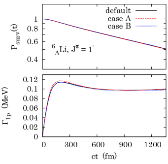
FIG. 4: Survival probability and resonance width of the 1p emission from the ground state of ${}^{6}_{\Lambda}$Li ($J^{\pi}=1^{-}$). The survival probability is plotted in the logarithmic scale. In the default case, $R_{\rm box}=120$ fm and $E_{\rm cut}=15$ MeV. In the case A, $R_{\rm box}=140$ fm and $E_{\rm cut}=15$ MeV. In the case B, $R_{\rm box}=120$ fm and $E_{\rm cut}=20$ MeV. The mean three-body energy is obtained as $E_{3b}=-2.521$, $-2.518$, and $-2.522$ MeV in the default case, case A, and case B, respectively.

Figure 4 shows the survival probability, $P_{surv}(t)$, and its decay width, $\Gamma_{\rm 1p}(t)$, for the $J^{\pi}=1^{-}$ configuration. These quantities are defined as the same in Refs. Maruyama et al. (2012); Oishi et al. (2014). From this result, the process is well interpreted as the exponential decay after sufficient time: $\Gamma_{\rm 1p}(ct>600~{}{\rm fm})\cong const$. The 1p-resonance width is suggested as $\Gamma_{\rm 1p}\cong 0.1$ MeV, when $E_{3b}=-2.5$ MeV consistent with the expected $Q_{\rm 1p}$ value, $0.6$ MeV.

Before closing this subsection, I show that the conclusion does not change even within the larger model space. In Fig. 4, in addition to the default setting with $E_{\rm cut}=15$ MeV and $R_{\rm box}=120$ fm, I repeat the same calculation but changing the cutoff parameters. In the case A, the radial box is extended as $R_{\rm box}=140$ fm, whereas the other parameters remain unchanged. In the case B, only the cutoff energy is increased as $E_{\rm cut}=20$ MeV. Consequently, in all the cases, the three-body energy and the 1p-emission width show a good coincidence. The deviation in the three cases is sufficiently smaller than the experimental uncertainties.

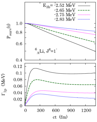
FIG. 5: Survival probability and resonance width of the 1p emission from the ${}^{6}_{\Lambda}$Li nucleus ($J^{\pi}=1^{-}$). Results with $a_{v}=-1.6$, $-1.8$, $-2.0$, and $-2.2$ fm, in correspondence to $E_{\rm 3b}=-2.52$, $-2.65$, $-2.75$, and $-2.83$ MeV, respectively, are presented. The survival probability is plotted in logarithmic scale.

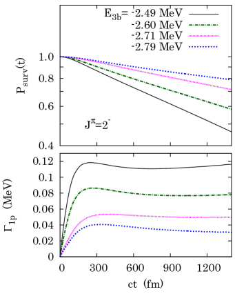
FIG. 6: Same to Fig. 5 but for the case of $J^{\pi}=2^{-}$. Results with $a_{v}=-1.6$, $-1.8$, $-2.0$, and $-2.2$ fm, in correspondence to $E_{\rm 3b}=-2.49$, $-2.60$, $-2.71$, and $-2.79$ MeV, respectively, are presented.

III.2 Sensitivity of 1p-resonance to proton-$\Lambda$ interaction

In this subsection, the sensitivity of the 1p-resonance energy and width is investigated. For this purpose, the proton-$\Lambda$ scattering length, $a_{v}$, is treated as the model parameter, which is associated with the bare strength of the proton-$\Lambda$ interaction.

Before going to the detailed discussion, I note the range of feasibility of the time-dependent method. Fortunately, in this paper, the $Q_{\rm 1p}$ value of interest yields the decay width, $\Gamma_{\rm 1p}$, of the order of $0.01-0.1$ MeV. In this case, after a sufficient time evolution, the time-dependent calculation fairly reproduces the exponentially decaying rule: $P_{surv}(t)\simeq P_{surv}(0)\exp\left(-t\Gamma_{\rm 1p}/\hbar\right)$, where $\Gamma_{\rm 1p}$ can be well constant. However, I also confirmed that, for the lower $Q_{\rm 1p}$ value, the decay width becomes inadequately small, and the time evolution should be performed to the long-time scale. At present, this calculation is impractical. To investigate this long-time scale, the computational improvement is necessary: the time-dependent method needs to be combined with, e.g. the absorption-boundary condition Mangin-Brinet et al. (1998); Schuetrumpf et al. (2016). On the other hand, for the larger $Q_{\rm 1p}$ value, the decay width becomes so large that it does not guarantee the valid picture of the quasi-stationary state: the state becomes much alike the scattering state, where the continuum effect should be more precisely taken into account. Also, in such a case, the survival probability does not form the exponential decay.

Figures 5 and 6 display the results of the survival probability and decay width. In this result, except $a_{v}$, the model parameters remain unchanged. There, in addition to the previous case, I test the new inputs, $a_{v}=-1.8,-2.0,$ and $-2.2$ fm. The three-body energy is obtained as $E_{3b}=-2.65,-2.75,$ and $-2.83$ MeV, respectively for $J^{\pi}=1^{-}$, whereas $E_{3b}=-2.60,-2.71,$ and $-2.79$ MeV, respectively for $J^{\pi}=2^{-}$. The resultant decay width shows a good convergence after a sufficient time evolution, indicating the exponential decay rule. These values are in the feasibility range of the time-dependent method. It is worthwhile to emphasize that the obtained decay width shows a noticeable fall from the 1p-resonance width of the hyperon-less $\alpha$-proton subsystem, $\Gamma_{\rm\alpha-p}\simeq 1.1$ MeV 02Till . Namely, the hyperon-inclusion remarkably affects the 1p-resonance observables.

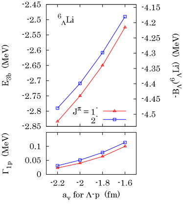
FIG. 7: (i) Top panel: three-body energies obtained with several values of the input parameter, $a_{v}$. The corresponding $-B_{\Lambda}(^{6}_{\Lambda}{\rm Li})$ values are presented in the right vertical axis according to Eq. (16). To convert from $E_{3b}$ to the $Q_{\rm 1p}$ value, see Eq. (15). (ii) Bottom panel: 1p-emission width of ${}^{6}_{\Lambda}$Li, obtained as the mean value during $ct=900-1200$ fm in Figs. 5 and 6.

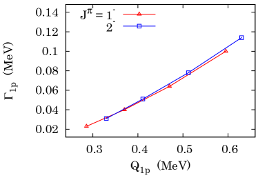
FIG. 8: One-proton resonance width as a function of the emitted $Q_{\rm 1p}$ value. From $E_{3b}$ values in Fig. 7, Eq. (15) is utilized to evaluate $Q_{\rm 1p}$.

In Fig. 7, the 1p-resonance observables as functions of the vacuum-scattering length, $a_{v}$, are summarized. Note that lowering the $a_{v}$ value leads to the enhancement of the attractive proton-$\Lambda$ force. This enhancement naturally yields the decrease of the three-body energy as well as the $Q_{\rm 1p}$ value. Also, the decrease of the width can be understood from the kinetic effect 2016KM . To show this kinetic effect better, in Fig. 8, the $Q_{\rm 1p}$-$\Gamma_{\rm 1p}$ relation is presented. It is clearly shown that, for the lower $Q_{\rm 1p}$ value, $\Gamma_{\rm 1p}$ becomes smaller, since the 1p penetrability via the core-proton potential barrier is more suppressed. Consequently, with the stronger attraction between proton-$\Lambda$, the system becomes more long-lived.

III.3 Spin-dependent splitting

In the previous subsection, the same parameter is used for the spin-singlet and spin-triplet proton-$\Lambda$ interactions. As the result, the splitting energy between the $1^{-}$ and $2^{-}$ resonances is much smaller than the expected value from the standard, spin-dependent YN interaction.

In this subsection, I extend the model to take the spin-dependence of the proton-$\Lambda$ interaction into account. For this purpose, instead of Eq. (6), I employ a spin-dependent contact interaction:

$$v_{\rm p-\Lambda}(\bm{r}_{\rm p},\bm{r}_{\Lambda})=\delta(\bm{r}_{\rm p}-\bm{r}_{\Lambda})\left[w^{(t)}_{0}\hat{P}_{t}+w^{(s)}_{0}\hat{P}_{s}\right],$$ (23)

where $\hat{P}_{s~{}(t)}$ indicates the projection to the spin-singlet (triplet) proton-$\Lambda$ configuration. Its strength parameters, $w^{(s)}_{0}$ and $w^{(t)}_{0}$, are determined from the spin-singlet and triplet scattering lengths, respectively. That is,

$$w^{(x)}_{0}=\frac{2\pi^{2}\hbar^{2}a^{(x)}_{v}}{\mu_{\rm p-\Lambda}(\pi-2a^{(x)}_{v}k_{\rm cut})}~{}~{}~{}~{}({\rm MeVfm^{3}}),$$ (24)

where $x=s$ or $t$.

For the input parameters, $(a^{(s)}_{v},a^{(t)}_{v})$, two cases as tabulated in TABLE 2 are compared: in the cases I and II, for the spin-singlet part, $a^{(s)}_{v}=-2.2$ fm and $-2.5$ fm, respectively. On the other hand, for the spin-triplet part, it is fixed as $a^{(t)}_{v}=-1.7$ fm in both cases. Namely, I consider the small (large) difference between the spin-singlet and triplet forces in the case I (II). These parameters are chosen consistently to the empirical results predicted by several YN interactions Gal et al. (2016); Nemura et al. (2002). Other parameters in the model remain unchanged.

TABLE 2: Input parameters of the vacuum-scattering lengths in the spin-singlet and triplet channels for the proton-$\Lambda$ contact interaction. The 1p-energy release, $Q_{\rm 1p}=-B_{\rm p}(^{6}_{\Lambda}{\rm Li})$, is evaluated from Eq. (15).

	$a^{(s)}_{v}$ (fm)	$a^{(t)}_{v}$ (fm)	$Q_{\rm 1p}$ (MeV)
			$J^{\pi}=1^{-}$	$J^{\pi}=2^{-}$
case I00	$-2.2$	$-1.7$	$+0.29$	$+0.53$
case II0	$-2.5$	(same)	$+0.22$	$+0.53$
case III	$\leq-4.0$	(same)	(bound)	$+0.53$

In TABLE 2, the resultant $Q_{\rm 1p}$ values are presented in the cases I and II. The mean three-body energy, $E_{3b}$, is obtained with the initial state, which is solved within the same confining potential in Sec. III.1. Consequently, in contrast to the previous results, now there is a noticeable splitting of the $1^{-}$ and $2^{-}$ 1p-resonance energies due to the spin-dependent proton-$\Lambda$ force. In the $J^{\pi}=1^{-}$ configuration, a noticeable sensitivity of the $Q_{\rm 1p}$ value (resonance energy) to the spin-singlet force is found: when $a^{(s)}_{v}$ becomes small, the $E_{3b}$ as well as $Q_{\rm 1p}$ gets decreased, consistently with that the spin-singlet proton-$\Lambda$ interaction, $w^{(s)}_{0}$, becoming more attractive. On the other hand, the result of the $J^{\pi}=2^{-}$ configuration is almost independent of the changes of the spin-singlet force. This can be understood from that, in the $(\kappa,\lambda)=(p_{3/2},s_{1/2})$ channel of the proton-$\Lambda$, only the spin-triplet configuration is allowed to couple to $J^{\pi}=2^{-}$. Indeed, this channel is dominant with $P(p_{3/2},s_{1/2})\simeq 98$% in both the cases I and II.

In Fig. 9, the 1p-emission width, $\Gamma_{\rm 1p}(t)$, from the time-dependent calculation is presented. First, in the $2^{-}$ configuration, as expected from the insensitivity of the $Q_{\rm 1p}$ value, the width is almost unchanged in the cases I and II: $\Gamma_{\rm 1p}\cong 75$ keV after the convergence at $ct\geq 600$ fm. In the $1^{-}$ configuration, on the other hand, $\Gamma_{\rm 1p}\cong 25$ and $15$ keV in the cases I and II, respectively. This sensitivity can be understood from the kinetic effect with the different $Q_{\rm 1p}$ values, as discussed in the last subsection. Notice that these predicted widths are comparably smaller than the splitting energy, $Q_{\rm 1p}(2^{-})-Q_{\rm 1p}(1^{-})\cong 200$ - $300$ keV, between the $1^{-}$ and $2^{-}$ states. Thus, there can be the two well-separated 1p-resonance levels in ${}^{6}_{\Lambda}$Li, which may provide suitable data to optimize the theoretical YN-interaction model with the spin-dependence.

Before closing the discussion, it is worth mentioning the last possible case, where the 1p emission is forbidden from the $1^{-}$ state, whereas it is still allowed from the $2^{-}$ state. For this condition, it requires $a^{(s)}_{v}\leq-4.0$ fm, whereas $a^{(t)}_{v}$ is kept as $-1.7$ fm. This set is listed as the case III in TABLE 2. In this case, as the result, $Q_{\rm 1p}<0$ for $J^{\pi}=1^{-}$, meaning that the 1p emission is not allowed. Namely, this spin-singlet force is sufficiently attractive to bind the valence proton. Consequently, if the spin-dependent splitting is sufficiently wide, the $1^{-}$ ground state of ${}^{6}_{\Lambda}$Li may be stable against the 1p emission. Note also that, even in this case, the 1p emission from the $2^{-}$ state can be still active, because of the insensitivity of the $Q_{\rm 1p}$ energy. Its width is also insensitive to $a^{(s)}_{v}$ as shown in Fig. 9.

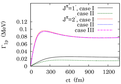
FIG. 9: The 1p-emission width of ${}^{6}_{\Lambda}$Li. These results are obtained with the sets of parameters, $(a^{(s)}_{v},a^{(t)}_{v})$, tabulated in TABLE 2. In the case III, 1p emission is forbidden from the $1^{-}$ ground state.

IV Summary

It is shown that the spontaneous-1p emission from ${}^{6}_{\Lambda}$Li can be sensitive to the proton-$\Lambda$ scattering length or its corresponding interaction strength. This sensitivity can be understood from the kinetic effect on the 1p-tunneling process via the core-proton potential. The proton-$\Lambda$ interaction, which is the novel ingredient in this hypernuclear system, can noticeably affect the 1p-emission observables, including the resonance energy and width, compared with the normal $\alpha$-proton resonance. By taking the spin-dependence of the proton-$\Lambda$ scattering length into account, a remarkable splitting of the $1^{-}$ and $2^{-}$ resonances is suggested. Utilizing the empirical spin-singlet and spin-triplet proton-$\Lambda$ scattering lengths as the model parameters, the decay widths of the two resonances are evaluated. From these suggestions, one may expect that the simultaneous 1p emission can be a suitable tool to investigate the YN-interaction properties.

It is worth mentioning that, from the resultant $\Gamma_{\rm 1p}$ value, the 1p emission from ${}^{6}_{\Lambda}$Li is suggested to occur in the timescale of $\tau=\hbar/\Gamma_{\rm 1p}\simeq 10^{-20}-10^{-21}$ seconds. This timescale is sufficiently shorter than the self-decay lifetime of $\Lambda$, $10^{-10}$ seconds. Thus, one can infer that the $\Lambda$ particle, as well as the daughter nucleus, ${}^{5}_{\Lambda}$He, is comparably unbroken during the emission process. This speculation, however, turns to be invalid in one exceptional case, where the proton-$\Lambda$ attraction is strong enough to prohibit the 1p emission.

In this paper, I utilized the simple three-body model. Compared with the ab initio multi-nucleon analysis Nemura et al. (2002); 2003Usm ; 2016Wirth ; 2016Gazda , this model includes several schematic parts. In forthcoming studies, I intend to combine the time-dependent method with the ab initio calculation, in order to investigate the particle-bound and unbound hypernuclei on equal footing. There are several topics, which can be addressed after this development. Those include, e.g., three-body hypernuclear interaction Nemura et al. (2002); 2003Usm ; 2016Wirth , spin-dependent charge-symmetry breaking 2016Gazda ; 2015Yama , and tensor force effect 04Ukai . How these effects are reflected on the nucleon-resonance properties can be a natural question following this first study. Also, the time-dependent calculation with the standard YN interaction model is an important future work.

For the first attempt to discuss the 1p emission with strangeness, the lightest hyper-1p emitter is investigated in this paper. In future studies, the similar interest can be widely devoted to the other systems along the proton-drip and neutron-drip lines, as well as the excited states of hypernuclei. For these systems, the structural model may need to be expanded: one has to implement the time-dependence into the four-or-more-particle model, or the fully microscopic-structure model. Several developments along this direction are in progress now.

*

Appendix A Transformation of coordinates

In the main text, the core-orbital coordinates are employed for the three-body system. In this Appendix, I give a basic formalism to determine these coordinates. It starts with the original coordinates and the conjugate momenta:

$$\vec{X}\equiv\left[\begin{array}[]{c}\bm{x}_{\rm p}\\ \bm{x}_{\Lambda}\\ \bm{x}_{\rm c}\end{array}\right],\qquad\vec{Q}\equiv\left[\begin{array}[]{c}\bm{q}_{\rm p}\\ \bm{q}_{\Lambda}\\ \bm{q}_{\rm c}\end{array}\right].$$ (25)

With these coordinates, the three-body Hamiltonian is trivially given:

$$H_{3b}=\sum_{i}\frac{\bm{q}_{i}^{2}}{2m_{i}}+V_{\rm c-p}+V_{\rm c-\Lambda}+v_{\rm p-\Lambda},$$ (26)

where $i={\rm p,\Lambda}$ and c for the valence proton, $\Lambda$, and the core, respectively.

With a $3\times 3$ matrix $U$, the core-orbital coordinates can be determined in the matrix form:

$$\vec{R}\equiv\left[\begin{array}[]{c}\bm{r}_{\rm p}\\ \bm{r}_{\Lambda}\\ \bm{r}_{G}\end{array}\right]=U\vec{X},\quad\vec{P}\equiv\left[\begin{array}[]{c}\bm{p}_{\rm p}\\ \bm{p}_{\Lambda}\\ \bm{p}_{G}\end{array}\right]=({}^{t}U)^{-1}\vec{Q},$$ (27)

where

$$U=\left(\begin{array}[]{ccc}1&0&-1\\ 0&1&-1\\ \frac{m_{\rm p}}{M}&\frac{m_{\Lambda}}{M}&\frac{m_{\rm c}}{M}\end{array}\right),$$ (28)

with $M\equiv\sum_{i}m_{i}$ (total mass). In these new coordinates, the Hamiltonian reads

$$H_{3b}=\frac{p_{G}^{2}}{2M}+\frac{p_{\rm p}^{2}}{2\mu_{\rm p}}+\frac{p_{\Lambda}^{2}}{2\mu_{\Lambda}}+\frac{\bm{p}_{\rm p}\cdot\bm{p}_{\Lambda}}{m_{\rm c}}+(potentials),$$ (29)

where the relative masses are given as $\mu_{i}=m_{i}m_{\rm c}/(m_{i}+m_{\rm c})$ for $i={\rm p}$ and $\Lambda$. The first term represents the center-of-mass kinetic energy. Since this center-of-mass term is well separated, one can obtain the three-body Hamiltonian in Eq. (1) correctly. Notice that the recoil term, $(\bm{p}_{\rm p}\cdot\bm{p}_{\Lambda})/m_{\rm c}$, should be always diagonalized, even if $v_{\rm p-\Lambda}$ is zero.

References

- Gal et al. (2016) A. Gal, E. V. Hungerford, and D. J. Millener, Rev. Mod. Phys. 88, 035004 (2016), and references therein.
- Feliciello and Nagae (2015) A. Feliciello and T. Nagae, Reports on Progress in Physics 78, 096301 (2015).
- Botta et al. (2012) E. Botta, T. Bressani, and G. Garbarino, The European Physical Journal A 48, 41 (2012).
- Rappold (2016) C. Rappold, Journal of Physics: Conference Series 668, 012025 (2016).
- Steinheimer et al. (2012) J. Steinheimer, K. Gudima, A. Botvina, I. Mishustin, M. Bleicher, and H. Stöcker, Physics Letters B 714, 85 (2012).
- Asai et al. (1984) F. Asai, H. Bandō, and M. Sano, Physics Letters B 145, 19 (1984).
- Baltz et al. (1994) A. Baltz, C. Dover, S. Kahana, Y. Pang, T. Schlagel, and E. Schnedermann, Physics Letters B 325, 7 (1994).
- (8) M. Pfützner et al., Eur. Phys. J. A 14, 279 (2002).
- (9) J. Giovinazzo et al., Phys. Rev. Lett. 89, 102501 (2002).
- Pfützner et al. (2012) M. Pfützner, M. Karny, L. V. Grigorenko, and K. Riisager, Rev. Mod. Phys. 84, 567 (2012).
- Grigorenko (2009) L. V. Grigorenko, Physics of Particles and Nuclei 40, 674 (2009).
- Motoba et al. (1983) T. Motoba, H. Bandō, and K. Ikeda, Progress of Theoretical Physics 70, 189 (1983).
- Hiyama et al. (1996) E. Hiyama, M. Kamimura, T. Motoba, T. Yamada, and Y. Yamamoto, Phys. Rev. C 53, 2075 (1996).
- Belyaev et al. (2008) V. Belyaev, S. Rakityansky, and W. Sandhas, Nuclear Physics A 803, 210 (2008).
- Hiyama and Yamada (2009) E. Hiyama and T. Yamada, Progress in Particle and Nuclear Physics 63, 339 (2009).
- (16) E. Hiyama et al., Phys. Rev. C 91, 054316 (2015).
- (17) S. A. Gurvitz, P. B. Semmes, W. Nazarewicz, and T. Vertse, Phys. Rev. A 69, 042705 (2004).
- Oishi et al. (2014) T. Oishi, K. Hagino, and H. Sagawa, Phys. Rev. C 90, 034303 (2014).
- Oishi et al. (2017) T. Oishi, M. Kortelainen, and A. Pastore, Phys. Rev. C 96, 044327 (2017).
- Ordonez and Hatano (2017) G. Ordonez and N. Hatano, Journal of Physics A: Mathematical and Theoretical 50, 405304 (2017).
- Ho (1983) Y. Ho, Physics Reports 99, 1 (1983).
- Michel et al. (2002) N. Michel, W. Nazarewicz, M. Płoszajczak, and K. Bennaceur, Phys. Rev. Lett. 89, 042502 (2002).
- Myo et al. (2014) T. Myo, Y. Kikuchi, H. Masui, and K. Kato, Progress in Particle and Nuclear Physics 79, 1 (2014).
- Grigorenko et al. (2000) L. V. Grigorenko, R. C. Johnson, I. G. Mukha, I. J. Thompson, and M. V. Zhukov, Phys. Rev. Lett. 85, 22 (2000).
- Bertsch and Esbensen (1991) G. Bertsch and H. Esbensen, Annals of Physics 209, 327 (1991).
- Esbensen et al. (1997) H. Esbensen, G. F. Bertsch, and K. Hencken, Phys. Rev. C 56, 3054 (1997).
- Hagino and Sagawa (2005) K. Hagino and H. Sagawa, Phys. Rev. C 72, 044321 (2005).
- (28) D. Tilley et al., Nucl. Phys. A 708, 3 (2002).
- (29) F. Ajzenberg-Selove, Nucl. Phys. A 490, 1 (1988). Note that several versions with the same title have been published.
- (30) “Chart of Nuclides” by National Nuclear Data Center (NNDC): http://www.nndc.bnl.gov/chart/.
- Gal (1975) A. Gal, Adv. Nucl. Phys. 8, 1 (1975).
- (32) R. Bertini et al., Nucl. Phys. A 368, 365 (1981).
- (33) H. Noumi et al., AIP Conf. Proc. 343, 703 (1995).
- (34) D.-M. Harmsen, Phys. Rev. Lett. 19, 1186 (1967); 19, 1409(E) (1967).
- Bhaduri and Nogami (1972) R. K. Bhaduri and Y. Nogami, Phys. Rev. Lett. 28, 1397 (1972).
- Goodhead and Evans (1967) D. T. Goodhead and D. A. Evans, Nucl. Phys. B 2, 121 (1967).
- Nemura et al. (2002) H. Nemura, Y. Akaishi, and Y. Suzuki, Phys. Rev. Lett. 89, 142504 (2002).
- Gurvitz and Kalbermann (1987) S. A. Gurvitz and G. Kalbermann, Phys. Rev. Lett. 59, 262 (1987).
- Gurvitz (1988) S. A. Gurvitz, Phys. Rev. A 38, 1747 (1988).
- Maruyama et al. (2012) T. Maruyama, T. Oishi, K. Hagino, and H. Sagawa, Phys. Rev. C 86, 044301 (2012).
- Jaganathen et al. (2017) Y. Jaganathen, R. M. Id Betan, N. Michel, W. Nazarewicz, and M. Płoszajczak, Phys. Rev. C 96, 054316 (2017).
- Bertulani et al. (2008) C. Bertulani, M. Hussein, and G. Verde, Physics Letters B 666, 86 (2008).
- Mangin-Brinet et al. (1998) M. Mangin-Brinet, J. Carbonell, and C. Gignoux, Phys. Rev. A 57, 3245 (1998).
- Schuetrumpf et al. (2016) B. Schuetrumpf, W. Nazarewicz, and P.-G. Reinhard, Phys. Rev. C 93, 054304 (2016).
- (45) Y. Kobayashi and M. Matsuo, Prog. Theor. Exp. Phys. 2016, 013D01 (2016).
- (46) A. A. Usmani and S. Murtaza, Phys. Rev. C 68, 024001 (2003).
- (47) R. Wirth and R. Roth, Phys. Rev. Lett. 117, 182501 (2016).
- (48) D. Gazda and A. Gal, Phys. Rev. Lett. 116, 122501 (2016).
- (49) T. O. Yamamoto et al., Phys. Rev. Lett. 115, 222501 (2015).
- (50) M. Ukai et al. (E930(’01) Collaboration), Phys. Rev. Lett. 93, 232501 (2004).