The Angular Size Distribution of $\mu$Jy Radio Sources

Abstract

We made two new sensitive (rms noise $\sigma_{\mathrm{n}}\approx\,1\,\mu$Jy beam${}^{-1}$) high resolution ($\theta=3\,\farcs 0$ and $\theta=0\,\farcs 66$ FWHM) S–band ($2<\nu<4$ GHz) images covering a single JVLA primary beam ($\mathrm{FWHM}\approx 14\arcmin$) centered on J2000 $\alpha=10^{\mathrm{h}}\,46^{\mathrm{m}}$, $\delta=+59^{\circ}\,01\arcmin$ in the Lockman Hole. These images yielded a catalog of 792 radio sources, $97.7\pm 0.8$% of which have infrared counterparts stronger than $S\approx 2\,\mu\mathrm{Jy}$ at $\lambda=4.5\,\mu\mathrm{m}$. About 91% of the radio sources found in our previously published, comparably sensitive low resolution ($\theta=8\arcsec$ FWHM) image covering the same area were also detected at $0\,\farcs 66$ resolution, so most radio sources with $S(3\,\mathrm{GHz})\gtrsim 5~{}\mu\mathrm{Jy}$ have angular structure $\phi\lesssim 0\,\farcs 66$. The ratios of peak brightness in the $0\,\farcs 66$ and $3^{\prime\prime}$ images have a distribution indicating that most $\mu$Jy radio sources are quite compact, with a median Gaussian angular diameter $\langle\phi\rangle=0\,\farcs 3\pm 0\,\farcs 1$ FWHM and an rms scatter $\sigma_{\phi}\lesssim 0\,\farcs 3$ of individual sizes. Most of our $\mu$Jy radio sources obey the tight far-infrared/radio correlation, indicating that they are powered by star formation. The median effective angular radius enclosing half the light emitted by an exponential disk is $\langle\rho_{\mathrm{e}}\rangle\approx\langle\phi\rangle/2.43\approx 0\,\farcs 12$, so the median effective radius of star-forming galaxies at redshifts $z\sim 1$ is $\langle r_{\mathrm{e}}\rangle\approx 1.0\mathrm{~{}kpc}$.

1 Introduction

We recently reported the results of a low-resolution ($\theta=8\arcsec$ FWHM) S-band ($2<\nu<4$ GHz) image made with the NRAO Karl G. Jansky Very Large Array (VLA) C configuration, covering a single primary beam (FWHM $\approx 14\arcmin$) centered on J2000 $\alpha=10^{\mathrm{h}}\,46^{\mathrm{m}}$, $\delta=+59^{\circ}\,01\arcmin$ in the Lockman Hole (Paper1; Paper2). The rms noise and confusion in this image are comparable: $\sigma_{\mathrm{n}}\approx\sigma_{\mathrm{c}}\approx 1~{}\mu\mathrm{Jy~{}beam}^{-1}$. The rapidly falling Euclidean-normalized differential source count $S^{5/2}n(S)$ at $\mu$Jy levels obtained from the confusion amplitude or “$P(D)$” distribution, converted to 1.4 GHz via the median spectral index $\langle\alpha\rangle=-0.7$, closely follows predictions of evolutionary models (Condon84; Wilman2008) in which most $\mu$Jy radio sources are powered by recent star formation in galaxies at median redshift $\langle z\rangle\sim 1$.

Our $\mu$Jy source count is much lower than that of OM2008, who derived a nearly constant $S^{5/2}n(S)$ from their sensitive 1.4 GHz VLA image made at the same position with $\theta=1\farcs 6$ resolution. OM2008 corrected their source count for the effects of partial resolution using a source angular-size distribution with median FWHM $\langle\phi\rangle\approx 1\farcs 2$ and a tail extending to much larger angular sizes. Paper1 detected all of the overlapping OM2008 sources, so it appears that the count correction required by the broad source angular-size distribution used is the primary cause of the higher OM2008 source count. A steep differential source count $n(S)\propto S^{-5/2}$ magnifies the impact of overestimated angular sizes on count corrections. A similar effect has appeared in numerous published source counts at sub-mJy levels, all of which were corrected for a range of assumed angular-size distributions and consequently disagree by amounts far greater than the published uncertainties (con07; Heywood2013).

F. Owen (private communication) recently made a sensitive VLA 1.5 GHz image ($\theta=1\farcs 6$ resolution, $\sigma=2.2\,\mu\mathrm{Jy~{}beam}^{-1}$ rms noise) of the GOODS-N field and found a typical FWHM source size $\langle\phi\rangle\sim 1\arcsec$. However, this result depends on data from a single VLA configuration and does not include multi-configuration images made with different VLA configurations and include tests using simulated data (of the type presented in Section LABEL:simulations) to demonstrate that the techniques used can robustly recover source sizes near or slightly below the instrumental resolution.

A sensitive high-resolution ($\theta\approx 0\,\farcs 22$) survey of the GOODS-N field using the VLA at 10 GHz (Murphy2017) recently detected a sample of 32 sources with a much smaller median angular diameter $\langle\phi\rangle=0\,\farcs 167\pm 0\,\farcs 032$ and rms size scatter $\sigma_{\phi}\approx 0\,\farcs 091$. Radio sources in star-forming galaxies are expected to be smaller at 10 GHz, owing to the stronger contribution of free-free emission, while the synchrotron radiation dominating at lower frequencies is spread out by cosmic-ray diffusion. However, the cosmic-ray diffusion is too small to grow sources from $0\,\farcs 17$ at 10 GHz to $1\arcsec$ at 1.5 GHz. Thus, there is still a significant spread in the reported median angular diameters of $\mu$Jy radio sources, and they remain disturbingly correlated with the resolution of the images used to find and fit Gaussians to the sources.

We believe that previous attempts to measure angular-size distributions and counts of faint radio sources have disagreed largely because: (1) they depended on sensitive images made with only a single high-resolution antenna configuration; (2) high-resolution images miss extended radio emission whose surface brightness is below the detection limit at that resolution; and (3) image noise tends to broaden Gaussians fitted to faint point sources by amounts proportional to the image resolution $\theta$. A more reliable method for constraining the angular-size distributions of source populations is to measure the peak flux densities (so-called “peak flux densities” are actually specific intensities written in units of flux density per beam solid angle; e.g., $\mu$Jy beam${}^{-1}$) in two or more images made with different array configurations, yielding different angular resolutions but similar point-source sensitivities. See Appendices B and C of Murphy2017 for a discussion of this method.

This paper presents two new S-band images made with $\theta=3\,\farcs 0$ and $\theta=0\,\farcs 66$ resolution from VLA B- and A-configuration data, respectively. Both are centered on J2000 $\alpha=10^{\mathrm{h}}\,46^{\mathrm{m}}$, $\delta=+59^{\circ}\,01\arcmin$. Extensive optical and infrared (IR) material on this field is available from Strazzullo2010, Mauduit2012, and Herschel160. Both images have $\sigma_{\mathrm{n}}\approx 1~{}\mu\mathrm{Jy~{}beam}^{-1}$ rms noise and negligible confusion. The new $3\arcsec$ and earlier $8\arcsec$ images yield accurate total flux densities because they do not resolve the vast majority of the $\mu$Jy source population, while the $\theta=0\,\farcs 66$ image should marginally resolve the $\phi\lesssim 0\,\farcs 5$ sources expected in the star-forming galaxies at redshifts $z\sim 1$ that dominate the $\mu$Jy source population (Condon84; Wilman2008).

An initial analysis of the source population found in our $8^{\prime\prime}$ resolution image was given in Paper3, who reported 10% radio-loud active galactic nuclei (AGNs), 28% radio-quiet AGNs, 58% star–forming galaxies, and 4% that could not be classified. Paper3 also gave a traditional discrete source count that needed little correction for partial resolution and agrees well with the deeper $P(D)$ analysis.

2 Observations

The dates and durations of our sensitive VLA S-band observations centered on J2000 $\alpha=10^{\mathrm{h}}\,46^{\mathrm{m}}$, $\delta=+59^{\circ}\,01\arcmin$ are summarized in Table 1. The C-configuration observations were described in Paper1, Paper2, and Paper3. The “B+” data were taken in the BnA configuration and during the transition to A configuration, but they had insufficient temporal or frequency resolution for the longer BnA baselines to be used in our highest-resolution ($\theta=0\,\farcs 66$) A-configuration image.

Table 1: Observations.

Array	Date Range	Time	No.
C	2012 Feb 21 – Mar 18	57.0	6
B+	2014 Feb 02 – Feb 18	26.0	10
A	2015 Jul 10 – Sep 13	39.4	6

“Array” is the VLA configuration. The start and end dates give the period over which the data were taken. “Time” is the total observing time in hours, and “No.” is the number of separate observing sessions. The “C” observations used the array prior to fully outfitting with 3 GHz receivers and included only 21 antennas.

The new A-configuration data have higher frequency resolution (500 kHz) and were recorded with shorter (1 s) basic integration times to minimize bandwidth- and time-smearing within the half-power circle of the VLA primary beam. The VLA correlator also separated the observed frequency range $1.989\leq\nu~{}\mathrm{(GHz)}\leq 4.013$ into 16 contiguous subbands of width $\Delta\nu=128$ MHz each. The A-configuration data processing was similar to that described in Paper1. Our flux-density calibration is based on a standard spectrum and model of 3C147 (PB2013A) and was transferred to the unresolved phase calibrator J1035+5628, whose absolute position uncertainty is $<0\,\farcs 002$. We used J1035+5628 to determine instrumental polarization and 3C147 (PB2013B) to calibrate the cross-polarized delays and phases. Calibration and editing used standard scripts in the Obit package (Obit). After calibration and extensive editing, the data were averaged over baseline-dependent time intervals chosen to minimize the size of the $(u,v)$ data set but avoid time smearing.

3 Imaging

We imaged the data sets using a joint multi-frequency CLEAN that both minimizes frequency dependent effects and exploits the full sensitivity of the wideband data. A single-resolution CLEAN was adequate for this field dominated by nearly unresolved sources. The low resoution image was imaged and restored using a $3\arcsec$ FWHM round, Gaussian beam and the high resolution data with a $0\,\farcs 66$ FWHM round, Gaussian beam. These values correspond to the resolution near the bottom of the ($2<\nu<4$ GHz) band. Briggs’ “optimal robust” weighting was used in the image formation (Briggs).

3.1 Wide-band, Wide-field Imaging

The large fractional bandwidth and wide field-of-view that was imaged require that both the source spectra and the antenna gain as a function of position and frequency be taken into account. This was done by the Obit task MFImage, which divides the observed spectrum into frequency bins narrow enough that the variations in antenna gain and spectral differences among sources are small within each bin. For this purpose, we set the frequency bin width equal to the 128 MHz correlator subband width.

The image was divided into a large number of small facet planes to minimize the effects of sky curvature. The facets were reprojected onto a common tangent plane and grid to allow parallel CLEANing. A frequency-dependent $(u,v)$ taper was applied to keep the angular resolution of the dirty beam the same in all frequency bins. This, plus the use of a single restoring beam, yields a meaningful 16-channel spectrum in each spatial pixel of the image cube.

For each major cycle of CLEAN, dirty and residual images were computed separately for each of the 16 frequency bins. The more sensitive full-bandwidth image, derived from the $\sigma_{i}^{-2}$ noise-weighted average of the frequency-bin images, was used to drive the minor cycle CLEANing. The sensitive combined image and the combined dirty beam were used to locate new CLEAN components, and the dirty beam for the corresponding frequency bin and facet was used to derive the residuals for the next minor cycle.

Once the minor cycles hit their stopping criteria, the accumulated CLEAN model was subtracted from the visibility data. The CLEAN model subtracted from each frequency bin used the CLEAN flux density of each component in that bin corrected in frequency by the spectral index fitted to each component using all frequency bins. This process was accelerated by a Graphics Processing Unit (GPU).

After the CLEANing was done, the image in each frequency bin was restored with the components subtracted from that bin convolved with the single Gaussian restoring beam fitted to the central facet of the combined full-sensitivity image.

This procedure accommodates variations with frequency of antenna gain and source flux density by using frequency bins sufficiently narrow that variations within a bin do not disturb the image quality. The spectrum in a given pixel depends on both antenna gain and source spectral index. The antenna gain as a function of position and frequency was measured independently (Perley16), allowing the spectral indices of sufficiently strong sources to be determined. For weaker sources, we used the average spectral index $\langle\alpha\rangle=-0.7$ to fit the source flux density at any frequency. That approximation is valid for most $\mu$Jy sources at S band.

Faraday rotation in the Stokes Q and U images is preserved if the frequency bins are sufficiently narrow and the rotation measure is not too large. A rotation measure $\mathrm{RM}=\pm 2000\mathrm{~{}rad~{}m}^{-2}$ rotates the polarization position angle by $1/2$ turn across a 128 MHz frequency bin at $\nu\approx 3\,\mathrm{GHz}$, so larger RMs than this will cause significant Faraday depolarization.

3.2 CLEAN Windows

CLEAN deconvolution works best if it is constrained to place components only in spatial “windows” containing actual emission. Our CLEAN windows were generated or updated at the beginning of each major cycle by the combined (wideband) image covering each facet. If the maximum residual lay outside the current window and its peak was higher than 5 times the facet rms, a new round window was added to the existing CLEAN window at the location of the peak, with a radius derived from the structure function about the peak. This allows CLEANing down to (or into) the noise and captures the bulk of the emission in the CLEAN model without producing excessive CLEAN bias.

3.3 Self-calibration

A single phase self-calibration was applied to the data. The model visibilities were calculated as was done in the CLEAN major cycles, and an independent phase solution was determined for each 10 minutes in each spectral window and polarization. These phases were interpolated in time and applied to all data.

3.4 Image Adjustments

The resulting images are 16 spectral-channel cubes covering $2<\nu\mathrm{(GHz)}<4$ that were jointly deconvolved and restored with a common spatial resolution. The sky brightness $S_{\mathrm{p}}(x,y)$ of the pixel offset by $(x,y)$ from the pointing center at the reference frequency $\nu_{0}=3$ GHz was calculated from the noise-weighted average of the spectral-window images:

$$S_{\mathrm{p}}(x,y)=\frac{\sum\limits_{i=1}^{16}{{S_{i}(x,y)\exp[{-\alpha{\rm ln}({\nu_{i}/{\nu_{0}}})}]}\over{g_{i}(x,y)}}{g^{2}_{i}(x,y)\over{\sigma^{2}_{i}}}}{\sum\limits_{i=1}^{16}{g^{2}_{i}(x,y)\over{\sigma^{2}_{i}}}}~{},$$ (1)

where $S_{i}(x,y)$ is the image (not corrected for primary-beam attenuation) brightness at pixel position $(x,y)$ in spectral channel $i$, $\alpha\approx-0.7$ is the median source spectral index, $\nu_{i}$ is the central frequency of spectral channel $i$, $0\leq g_{i}(x,y)\leq 1$ is the normalized antenna gain at offset $(x,y)$ from the pointing center and frequency $\nu_{i}$, and $\sigma^{2}_{i}$ is the mean variance of source-free regions in the $i$th spectral image. The first factor in the numerator of Equation 1 corrects the bin brightness $S_{i}(x,y)$ to the reference frequency using spectral index $\alpha$ and divides it by the primary attenuation $g_{i}(x,y)$ to yield the brightness on the sky $S_{\mathrm{p}}(x,y)$. The second factor is the pixel weight that maximizes the signal-to-noise ratio, specifically the antenna gain $g_{i}^{2}(x,y)$ divided by the spectral-channel image variance $\sigma_{i}^{2}$.

We approximated the normalized VLA antenna power gain $g_{i}(x,y)$ by the theoretical gain of a uniformly illuminated circular aperture:

$$g_{i}(\rho)=\mathrm{jinc^{2}}(D\rho/\lambda_{i})\equiv\Biggl{[}\frac{2J_{1}(\pi D\rho/\lambda_{i})}{\pi D\rho/\lambda_{i}}\biggr{]}^{2}~{},$$ (2)

where $\rho=(x^{2}+y^{2})^{1/2}$ is the offset from the pointing center in radians, $J_{1}$ is the Bessel function of the first kind of order 1 (Bracewell), $D=25\,\mathrm{m}$ is the aperture diameter, and $\lambda_{i}=c/\nu_{i}$ is the wavelength at the center frequency $\nu_{i}$ of spectral channel $i$. Equation 2 yields the primary beam FWHM $\theta_{1/2}$ in practical units; it is

$$\biggl{(}\frac{\theta_{1/2}}{\mathrm{arcmin}}\biggr{)}\approx 42.0\biggl{(}\frac{\mathrm{GHz}}{\nu}\biggr{)}~{},$$ (3)

which is only $\sim 1$% wider than the average beamwidth measured across S band (Perley16).

Applying Equation 1 corrects source flux densities for antenna gain but causes the image noise to increase radially as $g_{0}^{-1}(\rho)$ away from the pointing center. In order to determine meaningful noise statistics in the neighborhood of each source, we multiplied the gain-corrected image by the antenna gain $g_{0}(x,y)$ at the reference frequency $\nu_{0}=3$ GHz during source finding and fitting. For example, our $0\,\farcs 66$ resolution A-configuration image extends to a radius $\rho=8\,\farcm 3$. After multiplication by $g_{0}(\rho)$, its mean off-source rms is $\sigma=0.96~{}\mu$Jy beam${}^{-1}$.

We made a comparable image with $3\arcsec$ resolution and radius $\rho=13\,\farcm 8$ using the combined uvdata from the longer C-configuration baselines and the shorter BnA-configuration baselines (Table 1). Additionally, we convolved the A-configuration image to $3\arcsec$ resolution. Differences in celestial position and flux density scale of the two images were determined from the “at most” marginally resolved sources brighter than 100 $\mu$Jy beam${}^{-1}$. Finally, the B+C-configuration $3\arcsec$ image was shifted in position ($0\farcs 006$ in $\alpha$ and $-0\farcs 079$ in $\delta$) and scaled in flux density (0.933) to agree with the $3\arcsec$ A-configuration smoothed image, and the two $3\arcsec$ images were weighted by $\sigma^{-2}$ and combined. The differences in calibration are likely due to the extended period over which the B+C data were taken and the difficulties of calibration in a fierce RFI environment. The rms of the B+C image prior to primary beam correction was 1.27 $\mu$Jy beam${}^{-1}$ and for the A-configuration image convolved to $3\arcsec$ was 1.88 $\mu$Jy beam${}^{-1}$, giving relative weights of 70% and 30% respectively. Source-free regions in the final combined $3\arcsec$ image have rms $\sigma=1.01~{}\mu$Jy beam${}^{-1}$ prior to primary beam correction.

The $3\arcsec$ resolution image has imaging artifacts near the strongest source in the field, a hot spot in the lobe of an FR II source. To avoid contaminating the image statistics, we masked these artifacts by assigning affected pixels a value indicating that they should be ignored in subsequent analysis.

4 Radio Source Catalog

The Obit task FndSou was used to generate two independent lists of radio components from the wideband $\theta=3^{\prime\prime}$ and $\theta=0\,\farcs 66$ images, uncorrected for primary beam attenuation. FndSou locates “islands” of contiguous pixels brighter than a chosen peak flux density threshold and fits one or more elliptical Gaussian components to the emission in each island. These fits are subject to a number of constraints; in particular, any fitted Gaussian narrower than the (circular) CLEAN restoring beam is unphysical and was fitted by a Gaussian at least as wide as the restoring beam.

FndSou initially fits Gaussians in one island at a time and ignores overlapping components in adjacent islands. After the first component list for each image was generated, the parameters of potentially overlapping components were reconciled by refitting them jointly with all other components lying within 25 pixels ($2\,\farcs 3$ on the $\theta=0\,\farcs 66$ image or $11\farcs 0$ on the $\theta=3^{\prime\prime}$ image) in both $\alpha$ and $\delta$. The sky peak flux density $S_{\mathrm{p}}$ ($S_{\mathrm{p}}^{\mathrm{L}}$ for $\theta=3^{\prime\prime}$ and $S_{\mathrm{p}}^{\mathrm{H}}$ for $\theta=0\,\farcs 66$) of each Gaussian component was obtained by interpolating between image pixels to its fitted centroid position and dividing by the 3 GHz primary attenuation $g_{0}$ at that position. Interpolations used the Lagrangian technique with a $5\times 5$ kernel. Resolved sources represented by multiple components were replaced by only the component closest to the IR galaxy position; these six sources are discussed further in Section LABEL:extended.

The component lists from the $\theta=0\,\farcs 66$ and $\theta=3^{\prime\prime}$ images were merged to form a single list of source candidates lying inside the circle with 3 GHz primary attenuation $g_{0}>0.25$ (radius $10\farcm 1$). The candidate list includes:

1. all components from the $\theta=3^{\prime\prime}$ image with local signal-to-noise ratio $\mathrm{SNR}\equiv S_{\mathrm{p}}^{\mathrm{L}}/\sigma\geq 4$, plus

2. a small number of additional components with $\mathrm{SNR}\equiv S_{\mathrm{p}}^{\mathrm{H}}/\sigma\geq 5$ from the $\theta=0\,\farcs 66$ image.

For each of the candidate sources (item 1 above) the $\theta=0\,\farcs 66$ catalog was searched for nearby components with $S_{\mathrm{p}}^{\mathrm{H}}\geq 3\,\mu\mathrm{Jy~{}beam}^{-1}\approx 3\sigma$. An IR counterpart of each of the candidate sources was sought as described in Section 5.

From the candidate list, we kept as source components only:

1. the complete sample of 596 candidates with $\mathrm{SNR}\geq 5$ on the $\theta=3^{\prime\prime}$ image, plus

2. the reliable but incomplete sample of 156 candidates with $4\leq\mathrm{SNR}<5$ from the $\theta=3^{\prime\prime}$ image that were confirmed by an $S_{\mathrm{p}}^{\mathrm{H}}\gtrsim 3\sigma$ component lying within $3^{\prime\prime}$ on the $\theta=0\,\farcs 66$ image. (Excluding regions blocked by the bright IR sources, 88% of these also were within ${1\farcs 5}$ of an IR source.) Plus

3. the additional 40 candidates with $4\leq\mathrm{SNR}<5$ from the $\theta=3^{\prime\prime}$ image that were confirmed only by an IR source lying within ${1\farcs 5}$ ( see below).

Our final catalog contains 792 radio source components, a sample of which is shown in Table 2; the full table is available online. At $\mu$Jy levels there are very few resolved double radio sources, so nearly every cataloged radio source component is also a complete astrophysical radio source, defined as all of the radio emission from a single galaxy or AGN. Of the 209 source candidates from the $\theta=3^{\prime\prime}$ image with $4\leq\mathrm{SNR}<5$ and in locations where an IR identification was possible, only 14 had neither an IR identification nor a radio counterpart on the $\theta=0\,\farcs 66$ image. 75% of these (154/205) were within ${1\,\farcs 5}$ of an IR source and outside of areas blocked by the brighter IR sources (see below).

Table 2: Source Catalog.

J2000 $\alpha$	J2000 $\delta$	$\theta$	$g_{0}$	$S_{\mathrm{p}}^{\mathrm{L}}$	$~{}S^{\mathrm{L}}$	L$-$H	$S_{\mathrm{p}}^{\mathrm{H}}$	$~{}S^{\mathrm{H}}$	$\phi$	$r$
h  m  s            s	${}^{\circ}$  ${}^{\mathrm{m}}$  ${}^{\prime\prime}$          ${}^{\prime\prime}$			($\mu$Jy beam${}^{-1}$)	($\mu$Jy)	(${}^{\prime\prime}$)	($\mu$Jy beam${}^{-1}$)	($\mu$Jy)	(${}^{\prime\prime}$)	(${}^{\prime\prime}$)
10 44 43.071 $\pm$ 0.071	58 59 51.05 $\pm$ 0.55	L	0.26	19.49 $\pm$ 3.98	25.70 $\pm$ 5.76	4.53				1.10
10 44 44.109 $\pm$ 0.009	59 00 19.36 $\pm$ 0.07	H	0.27	16.96 $\pm$ 4.02	16.00 $\pm$ 3.82	0.20	21.18 $\pm$ 3.31	20.66 $\pm$ 3.29	$<0.61$	0.24
10 44 46.577 $\pm$ 0.015	58 58 40.70 $\pm$ 0.11	H	0.28	14.96 $\pm$ 3.66	14.06 $\pm$ 3.47	0.35	12.07 $\pm$ 3.30	11.17 $\pm$ 3.07	$<0.86$	0.24
10 44 46.940 $\pm$ 0.007	59 01 56.37 $\pm$ 0.04	H	0.30	39.90 $\pm$ 3.46	44.51 $\pm$ 4.26	0.13	33.50 $\pm$ 3.01	33.23 $\pm$ 3.15	$<0.45$	0.50
10 44 47.417 $\pm$ 0.013	58 58 01.79 $\pm$ 0.10	H	0.27	18.33 $\pm$ 3.76	17.56 $\pm$ 3.64	0.23	13.59 $\pm$ 3.25	12.82 $\pm$ 3.09	$<0.79$	0.18
10 44 47.563 $\pm$ 0.006	58 59 18.74 $\pm$ 0.03	H	0.30	49.70 $\pm$ 3.60	49.44 $\pm$ 3.88	0.13	55.51 $\pm$ 3.04	55.34 $\pm$ 3.45	$<0.36$	0.29
10 44 47.661 $\pm$ 0.005	59 00 35.66 $\pm$ 0.03	H	0.31	88.76 $\pm$ 3.61	91.48 $\pm$ 4.67	0.06	79.23 $\pm$ 3.02	80.61 $\pm$ 3.93	$<0.33$	0.38
10 44 47.725 $\pm$ 0.018	59 02 14.60 $\pm$ 0.14	H	0.31	34.85 $\pm$ 3.39	35.53 $\pm$ 3.66	0.82	11.34 $\pm$ 3.04	12.69 $\pm$ 3.66	$<1.15$	0.83
10 44 47.794 $\pm$ 0.012	58 58 12.47 $\pm$ 0.08	H	0.28	19.53 $\pm$ 3.69	19.97 $\pm$ 3.93	0.54	15.82 $\pm$ 3.22	15.16 $\pm$ 3.12	$<0.72$	0.77
10 44 49.188 $\pm$ 0.014	58 57 19.82 $\pm$ 0.10	H	0.27	17.85 $\pm$ 3.82	17.04 $\pm$ 3.68	0.65	12.71 $\pm$ 3.28	11.86 $\pm$ 3.08	$<0.83$	0.47

Note. — Table 2 is published in its entirety in machine-readable format. A portion is shown here for guidance regarding its form and content. The table lists J2000 right ascensions $\alpha$ and declinations $\delta$ measured from the $\theta=0\,\farcs 66$ resolution image if available (indicated by “H” in the $\theta$ column), otherwise from the $\theta=3^{\prime\prime}$ resolution image (“L” in the $\theta$ column). Interpretation of the fitted Gaussian parameters follows the development in (con97). The rms position errors include our estimated absolute astrometric uncertainty $\sigma_{\alpha}=\sigma_{\delta}\approx 0\,\farcs 02$. Column $g_{0}$ gives the normalized antenna gain at the source position. The 3 GHz peak and total flux densities corrected for fitting bias (con97) from the low-resolution image are listed under $S_{\mathrm{p}}^{\mathrm{L}}$ and $S^{\mathrm{L}}$. L$-$H is the separation of the positions measured on the low- and high-resolution images. $S_{\mathrm{p}}^{\mathrm{H}}$ and $S^{\mathrm{H}}$ are the peak and integrated flux densities from the high-resolution image. Column $\phi$ gives the deconvolved Gaussian source FWHM sizes or upper limits at $0\,\farcs 66$ resolution. Next, $r$ is the angular distance between the radio source and its nearest IR neighbor. Separations less than $1\,\farcs 5$ are considered solid associations, $1\,\farcs 5$ $\leq r\leq$ $3\,\farcs 5$ are probable associations, and $r>3\,\farcs 5$ are unassociated.

5 Radio/IR Identifications

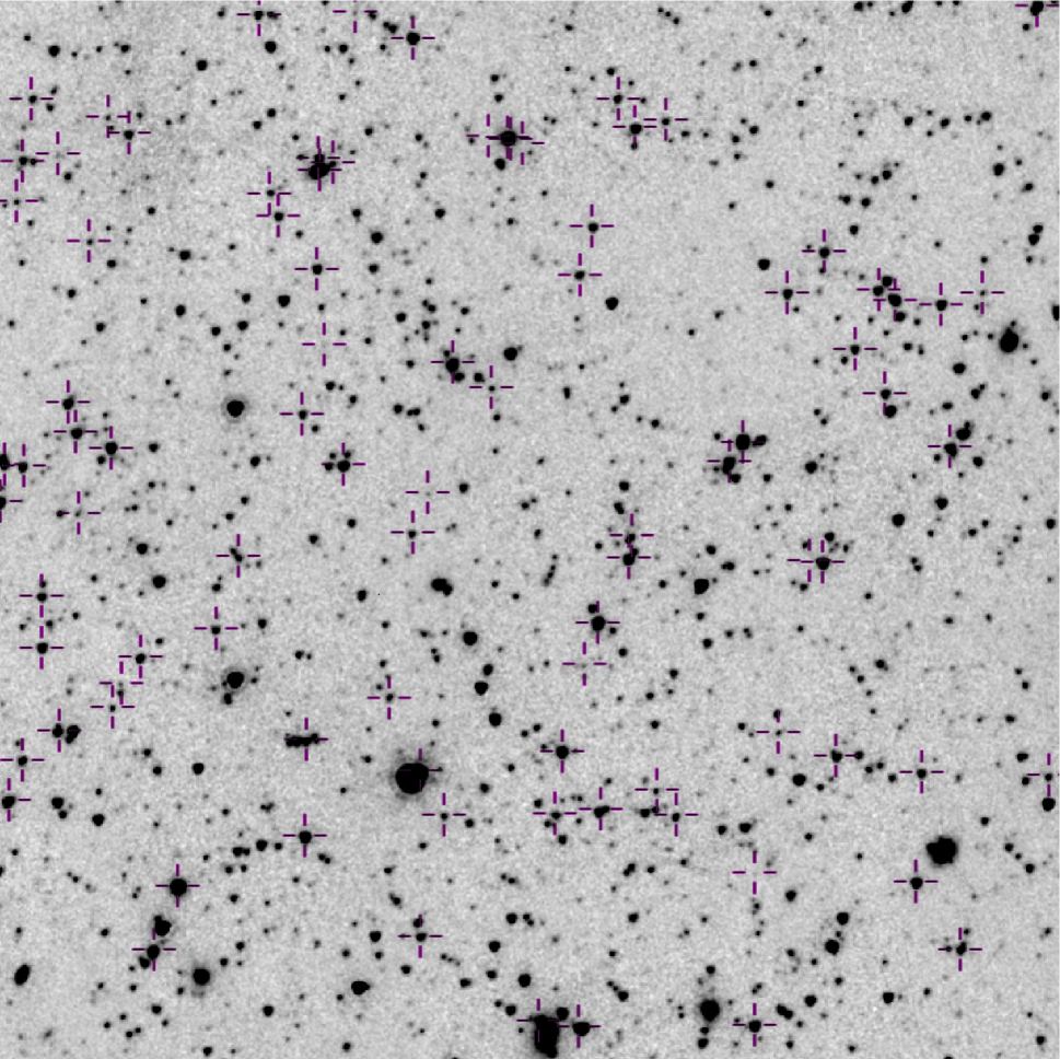
Figure 2: Radio positions marked by crosses on negative gray scale of the $\lambda=4.5\,\mu$m Spitzer image. The area shown is $7\,\farcm 2\times 7\,\farcm 0$, with north up and east to the left; this is only a portion of the field imaged.

Most of our cataloged radio sources are powered by star-forming galaxies and AGNs that should be visible in sensitive IR images. Deep $\lambda=3.6\,\mu\mathrm{m}$ and $\lambda=4.5\,\mu\mathrm{m}$ images from the Spitzer Extragalactic Representative Volume Survey (SERVS) (Mauduit2012) cover the entire area we imaged at S–band, although part of the overlapping IR image is blinded by scattered light from the very bright star GX UMa at J2000 $\alpha=10^{\mathrm{h}}\,46^{\mathrm{m}}\,07\,\fs 70$, $\delta=+59^{\circ}\,03\arcmin\,39\,\farcs 2$. Furthermore, the Mauduit2012 IR catalog excludes small regions around moderately bright foreground stars in which galaxies are still visible. We excluded from our radio/IR comparisons only the 48 sources in regions that are actually blinded by bright stars and kept as identification candidates all visible IR galaxies that had been excluded from the Mauduit2012 catalog. At both $\lambda=3.6\,\mu\mathrm{m}$ and $\lambda=4.5\,\mu\mathrm{m}$ the Mauduit2012 catalog $5\sigma$ point-source detection limit is $S\approx 2\,\mu$Jy and the IR images have FWHM resolution $\theta\approx 2^{\prime\prime}$. The Spitzer $\lambda=4.5\,\mu$m image in Figure 2 shows that nearly all of our radio source positions (crosses) have IR identifications.

Figure 1: Left panel: Histogram of measured radial offsets $r$ between points on an arbitrary grid of $120\times 120$ positions separated by $10^{\prime\prime}$ and their nearest IR neighbors. The data are well fit by the Rayleigh distribution (smooth curve) with rms $\sigma=3\,\farcs 35$, expected for randomly scattered IR sources with mean sky density $\rho=0.0142\mathrm{~{}arcsec}^{-2}$. Right panel: Histogram of measured radial separations $r$ between radio sources in Table 2 (excluding the IR-blinded fields and the faint sources kept only because they have IR counterparts within $1\farcs 5$) and their nearest IR neighbors. The core of this distribution can be approximated by a Rayleigh distribution with rms $\sigma\approx 0\,\farcs 22$, but there is a tail of somewhat larger offsets, many of which are genuine radio-IR matches. Abscissae: Angular distance (arcsec) between a radio source and its nearest IR neighbor. Ordinates: Probability density (arcsec${}^{-1}$).

We identified Spitzer IR sources with radio sources in Table 2 on the basis of position coincidence: the IR source nearest to the radio source was accepted as the identification if it lies within our maximum search radius $r_{\mathrm{s}}$. The probability that an unrelated IR source will incorrectly be identified depends on the radio and IR position uncertainties and on the sky density $\rho$ of IR identification candidates. The left panel of Figure 1 shows a histogram of radial distances $r$ to the IR sources nearest to an arbitrary grid of $120\times 120=14400$ positions spaced by $10^{\prime\prime}$ in right ascension and declination. The histogram is well approximated by the expected Rayleigh distribution

$$P(r)=\frac{r}{\sigma^{2}}\exp\biggl{(}-\frac{x^{2}}{2\sigma^{2}}\biggr{)}=2\pi\rho r\exp(-\pi\rho r^{2})~{},$$ (4)

where $\sigma\approx 3\,\farcs 35$ is the fitted rms width of the distribution and $\rho=(2\pi\sigma^{2})^{-1}\approx 0.0142\mathrm{~{}arcsec}^{-2}$ is the implied sky density of IR sources.

This result can be used to calculate how strongly having IR companions within $1\farcs 5$ confirms the reality of the 40 faint ($4\leq\mathrm{SNR}<5$) sources found only on the $\theta=3^{\prime\prime}$ radio image. The cumulative Rayleigh distribution

$$P(<r)=1-\exp\biggl{(}-\frac{r^{2}}{2\sigma^{2}}\biggr{)}~{}$$ (5)

specifies the probability that an unrelated IR source lies within a distance $r$ from any point on the sky. For $\sigma=3\,\farcs 35$, the probability that a spurious radio source would have an IR companion within $1\farcs 5$ is $P(<1\farcs 5)\approx 0.095$, so an IR confirmation boosts the reliability of a $4\leq\mathrm{SNR}<5$ radio source by a factor of $0.095^{-1}\sim 10$.

The offsets $r$ of most genuine radio/IR identifications should have a roughly Rayleigh distribution whose rms is the quadratic sum of the radio position error, the IR position error, and any radio-IR offset intrinsic to the host galaxy. The distribution of IR offsets from the radio positions of the 752 radio sources not confirmed only by an IR source lying within $1\farcs 5$ is shown by the histogram in the right panel of Figure 1, and the continuous curve fitting most sources is a Rayleigh distribution with $\sigma\approx 0\,\farcs 22$. However, there is a tail of sources with offsets too large to be consistent with this Rayleigh distribution yet too small to be explained by the Rayleigh distribution of unrelated sources shown in the left panel. Such tails are not rare (e.g., Murphy2017) and can be attributed to a few sources with larger combined position errors, extended galaxies with genuine IR-radio offsets, sources in clusters and a small contamination by unrelated IR sources.

To determine the optimum search radius $r_{\mathrm{s}}$ that will accept most genuine identifications and minimize contamination by unrelated IR sources, we exploited the fact that all unrelated sources should obey the Rayleigh offset distribution with $\sigma=3\,\farcs 35$ shown in the left panel of Figure 1. The fraction of background sources with $r>\sigma=3\,\farcs 35$ is $P(>r)=1-P(<r)\approx 0.606$. On the conservative assumption that all 10 sources with $r>\sigma=3\,\farcs 35$ in our catalog are unrelated to their IR neighbors, the total number of unrelated IR sources with any $r>0$ should be $N_{\mathrm{u}}\approx(10\pm 3)/0.606\approx 16.5\pm 5$. Excluding the 40 faint sources cataloged only because they have IR identifications and the 48 unidentifiable sources in regions overwhelmed by bright IR stars, Table 2 contains an IR-unbiased sample of 704 radio sources of which $\approx(704-16.5)/704=97.7\pm 0.8$% have true IR identifications stronger than $S\approx 2\,\mu$Jy at $\lambda=4.5\,\mu$m. This high radio/IR identification rate also indicates that $\lesssim 2$% of the cataloged radio sources can be spurious.

The expected numbers of background sources in different ranges of $r$ can be calculated from Equation 5 and compared with the observed numbers plotted in the right panel of Figure 1 to estimate the reliability $R$ of an identification as a function of $r$, as shown in Table 3. For $r<1^{\prime\prime}$, $R\approx 1$. In the range $1\arcsec<r<1\farcs 5$, the average number of unrelated background sources $\langle N_{\mathrm{u}}\rangle\approx 0.85$ is much smaller than the observed number $N_{\mathrm{o}}=23$ of radio/IR matches, suggesting that $R\approx(N_{\mathrm{o}}-\langle N_{\mathrm{u}}\rangle)/N_{\mathrm{o}})\approx 0.96$. Thus a search radius $r_{\mathrm{s}}=1\farcs 5$ should yield highly reliable radio/IR identifications. Table 3 shows how reliability decreases for larger separations. Nevertheless, more than half of the “probable” identifications with $1\,\farcs 5<r<3\,\farcs 5$ appear to be correct.

Table 3: IR identification reliability. $R$

$~{}r(^{\prime\prime})$	$\langle N_{\mathrm{u}}\rangle$	$N_{\mathrm{o}}$	$R$
1.0–1.5	0.85	23	0.96
1.5–2.0	1.12	28	0.86
2.0–2.5	1.32	29	0.85
2.5–3.0	1.44	25	0.71
3.0–3.5	1.49	24	0.63

Notes: For each radio-IR offset range $r$, $\langle N_{\mathrm{u}}\rangle$ is the average number of unrelated IR sources, $N_{\mathrm{o}}$ is the observed number of IR sources, and $R$ is the estimated identification reliability.

Let $m\equiv r_{\mathrm{s}}/\sigma$ be the search radius in units of the rms position error $\sigma\approx 0\,\farcs 22$ and define $k\equiv 1+2\pi\rho\sigma^{2}\approx 1.0043$. Then the completeness $C$ of our position-coincidence identifications is

$$C=\frac{1-\exp(-m^{2}k/2)}{k}\approx 0.996$$ (6)

and the reliability $R$ is

$$R=C\biggl{[}\frac{1}{f}-\biggl{(}1-\frac{1}{f}\biggr{)}\exp[m^{2}(1-k)/2)]-$$

$$\exp\biggl{(}-\frac{m^{2}k}{2}\biggr{)}\biggr{]}^{-1}\approx 0.957~{}~{}~{}~{}~{}$$ (7)

(condonetal75).

6 Source Size Distribution

Most of the individual fitted Gaussian sizes produced in the source-finding process are sufficiently uncertain to yield only upper limits to the individual deconvolved source sizes. However, the mean ratio $\langle S_{\mathrm{p}}^{\mathrm{H}}/S_{\mathrm{p}}^{\mathrm{L}}\rangle$ of the fitted peak brightness $S_{\mathrm{p}}^{\mathrm{H}}$ (on the $\theta_{\mathrm{H}}=0\,\farcs 66$ high-resolution image) to $S_{\mathrm{p}}^{\mathrm{L}}$ (on the $\theta_{\mathrm{L}}=3\arcsec$ low-resolution image) depends on the source solid angle. If a circular Gaussian source of FWHM diameter $\phi$ and flux density $S$ is imaged with a beam of FWHM diameter $\theta$, the source appears on the image as a circular Gaussian with FWHM diameter $(\theta^{2}+\phi^{2})^{1/2}$ and peak brightness

$$S_{\mathrm{p}}=S\biggl{(}\frac{\theta^{2}}{\theta^{2}+\phi^{2}}\biggr{)}~{}.$$ (8)

If the circular Gaussian source is imaged with two different resolutions $\theta_{\mathrm{H}}$ and $\theta_{\mathrm{L}}$, the ratio of the image peak brightnesses is

$$\frac{S_{\mathrm{p}}^{\mathrm{H}}}{S_{\mathrm{p}}^{\mathrm{L}}}=\biggl{(}1+\frac{\phi^{2}}{\theta_{\mathrm{L}}^{2}}\biggr{)}\biggl{(}1+\frac{\phi^{2}}{\theta_{\mathrm{H}}^{2}}\biggr{)}^{-1}~{}.$$ (9)

Appendix C of Murphy2017 gives the $S_{\mathrm{p}}^{\mathrm{H}}/S_{\mathrm{p}}^{\mathrm{L}}$ ratio for a source with the exponential brightness profile typical of spiral galaxies. Equation 9 can be solved for the source size $\phi$:

$$\phi=\Biggl{[}\frac{\theta_{\mathrm{L}}^{2}\theta_{\mathrm{H}}^{2}(S_{\mathrm{p}}^{\mathrm{L}}-S_{\mathrm{p}}^{\mathrm{H}})}{\theta_{\mathrm{L}}^{2}S_{\mathrm{p}}^{\mathrm{H}}-\theta_{\mathrm{H}}^{2}S_{\mathrm{p}}^{\mathrm{L}}}\Biggr{]}^{1/2}~{}.$$ (10)

Even if a source does not have a circular Gaussian brightness distribution, Equation 10 defines what we call its equivalent source circular Gaussian FWHM.

Equations 9 and 10 allow us to estimate the statistical properties of the source sizes in our sample. The distribution of $S_{\mathrm{p}}^{\mathrm{H}}/S_{\mathrm{p}}^{\mathrm{L}}$ as a function of $S_{\mathrm{p}}^{\mathrm{L}}$ is given in Figure LABEL:RatioVFlux. Sources with and without IR counterparts are shown by different symbols. Horizontal lines give the expected values for circular Gaussians of various FWHM diameters $\phi$.

The cataloged sources were separated into peak brightness bins in which the bin-averaged peak brightnesses and peak brightness ratios are plotted in Figure LABEL:RatioVFlux with “error bars” giving the rms ratio for the population in each bin. The peak brightness bin statistics are given in Table 4. Outliers further from from the initial mean by more than 2 $\sigma$ were excluded from the analysis of bin popluations.

At peak brightnesses below the 20–30 $\mu$Jy beam${}^{-1}$ bin, the distribution of peak brightness ratios appears truncated on the low end by limited sensitivity. The 20–30 $\mu$Jy beam${}^{-1}$ and higher peak brightness bins in Table 4 consistently give an equivalent source circular Gaussian FWHM of $\theta\approx 0\,\farcs 3$.

Table 4: Measured average ratios of peak flux densities.

No.	$\langle S_{\mathrm{p}}^{\mathrm{L}}\rangle$	$\langle S_{\mathrm{p}}^{\mathrm{H}}/S_{\mathrm{p}}^{\mathrm{L}}\rangle$	$\sigma_{\rm pop}$	FWHM	err
	$\mu$Jy			$\arcsec$	$\arcsec$
428	2 6.4	0.76	0.18	0.39	0.19
165	13.9	0.71	0.19	0.43	0.21
52	24.3	0.69	0.25	0.45	0.27
31	37.4	0.77	0.18	0.38	0.19
14	58.3	0.87	0.11	0.26	0.13
9	83.8	0.93	0.07	0.20	0.09

Notes: “No.” is the number of sources in the bin, excluding outliers, $\langle S_{\mathrm{p}}^{\mathrm{L}}\rangle$ is the average peak brightness at $3\arcsec$ resolution, $\langle S_{\mathrm{p}}^{\mathrm{H}}/S_{\mathrm{p}}^{\mathrm{L}}\rangle$ is the average peak brightness ratio, $\sigma_{\rm pop}$ is the rms ratio of the bin sample, “FWHM” is the equivalent half-power diameter of a circular Gaussian with the ratio of the bin average, and “err” is the estimated 1 $\sigma$ error of “FWHM”.