Linear response approach to active Brownian particles in time-varying activity fields

Abstract

In a theoretical and simulation study, active Brownian particles (ABPs) in three-dimensional bulk systems are exposed to time-varying sinusoidal activity waves that are running through the system. A linear response (Green-Kubo) formalism is applied to derive fully analytical expressions for the torque-free polarization profiles of the particles. The activity waves induce fluxes that strongly depend on the particle size and may be employed to de-mix mixtures of ABPs or to drive the particles into selected areas of the system. Three-dimensional Langevin dynamics simulations are carried out to verify the accuracy of the linear response formalism, which is shown to work best when the particles are small (i.e. highly Brownian) or operating at low activity levels.

I Introduction

Biological systems often contain microscopic objects of different sizes, featuring a self-propulsion to play a crucial role in vital actions. Prominent examples are white blood cells chasing intruders fenteany_COH04 , motor proteins facilitating the transport of e.g. RNA inside cells kanai_Neuron04 , or bacteria such as Escherichia coli which are simply searching for food berg_04 .

On the other hand, synthetic microswimmers are designed to offer hope-bearing solutions to problems that are hard to approach with the toolbox available to conventional nanotechnology ebbens_SM10 ; yamamoto_powder15 . Potential fields of applications are highly directional drug delivery, improved biomarkers or contrast agents abdelmohsen_JMCB14 , as well as the elimination of pollutants in the framework of environmental protection gao_ACSNano14 .

By far the simplest synthetic self-propelling agents are binary Janus-particles of spherical shape. These particles may be driven by catalytic reactions with an ingredient of the solvent such as hydrogen peroxide howse_PRL07 or hydrazine gao_JACS14 . If the ’fuel’ exhibits a concentration gradient, then the activity of these ABPs turns position dependent, leading to phenomena that have recently been demonstrated to resemble chemotaxis peng_AC15 ; ghosh_PRE15 ; vuijk_18 . Instead of being chemically driven, Janus particles may also respond to light as a result of an inhomogeneous surface-heating and the resulting local temperature gradient lozano_NatureComm16 . This resembles phototactic behavior, and since light intensities are easily controlled in a laboratory setup, not only position-, but also rapidly varying time-dependent activity profiles may be employed to manipulate ABPs. Recent reviews about the state of the art of artificial nano motors have been presented by Yamamoto et al. yamamoto_powder15 and Bechinger et al. bechinger_RevModPhys16 .

Some of the authors have recently applied the linear response (Green-Kubo) approach to ABPs and successfully computed average swim speeds sharma_JCP16 in homogeneous systems as well as a torque-free polarization and the resulting density distributions in systems with spatially inhomogeneous activity profiles sharma_PRE17 . In the present work, we generalize that formalism to systems in which the activity fields are additionally time dependent. Recently, Geiseler et al. have analyzed the behavior of microswimmers in active density waves that are sweeping over the ABPs and thereby driving them into selected directions geiseler_PRE16 ; geiseler_SR17 . Techniques to manipulate the global direction of motion of ABPs are naturally of paramount interest to the practitioner. While existing studies are restricted to two-dimensional setups and thus affected by boundary effects of the substrate on which the particles are sliding, our linear response approach is going to be applied to three dimensional bulk systems in absence of boundaries.

In Sec. II, we first present our model, the system of units and a short introduction to linear response theory. Section III derives the orientation profiles of ABPs that are exposed to a propagating sinusoidal activity wave. The resulting torque-free polarization profile inside the activity gradient is derived as a fully analytical expression and compared to Langevin dynamics simulations. The corresponding density distributions are derived in Sec. IV and again a close agreement with the simulations is reported. Section V studies the fluxes induced into the ABPs by the propagating activity wave, which strongly depend on the particle size. This fact is exploited in Sec. VI in which a mixture of ABPs of different sizes is de-mixed by selective applications of induced fluxes. We discuss the parameter ranges in which the linear response ansatz yields accurate predictions (Sec. VII) and summarize our findings in VIII.

II Model and Theory

II.1 Numerical simulations

In this work, we introduce a standard particle with a diameter of $b=1$ and mass $m=1$, which define the length and mass units. We explicitly specify the translational diffusion coefficient $D_{t}=k_{B}T/\zeta$ and the drag coefficient $\zeta$, and with $k_{B}=1$, the unit-less temperature of the system is specified, too. The unit time $\tau$ is the time which the standard particle needs to diffuse over the distance of its diameter, i.e. $\tau=(6D_{t})^{-1}$. We have thus scaled the remaining parameters to yield $\tau=1$.

The Langevin dynamics simulations were carried out with the molecular dynamics simulation package LAMMPS plimpton_CompPhys95 in fully three dimensional setups. The activity is induced by an explicit force that acts in the direction of the particle’s internal orientation vector, noise is induced by a Langevin thermostat at a system temperature of $T=5/3$. We use an integration time-step of $4\cdot 10^{-4}$. In the simulations of sections III – V, 500 active particles are placed into a box of the size $L^{3}=15^{3}$ and periodic boundaries. The particles have a diameter of $b=1$, but no interaction, so that actually an ensemble of single particles is simulated. In Sec. VI, particles of different diameters are distributed inside a larger box of size $15\times 15\times 150$, being bounded in z-direction with impenetrable walls, but periodic in x- and y-directions. The remaining parameters are summarized in Tab. 1. Further technical details regarding the implementation of ABPs in LAMMPS have been described in our previous publication merlitz_SM17 .

diameter, $b$	0.5	1	2
mass, $m$	1/8	1	8
frictional drag coefficient, $\zeta$	5	10	20
momentum relaxation time, $\tau_{m}$	1/40	1/10	2/5
translational diffusion coefficient, $D_{t}$	1/3	1/6	1/12
rotational diffusion coefficient, $D_{r}$	4	1/2	1/16
rotational relaxation time, $\tau_{r}$	1/8	1	8
ratio, $\tau_{r}/\tau_{m}$	5	10	20

Table 1: Simulation parameters for ABPs of different diameter $b$. The mass $m$ is required for the integrator, but the resulting momentum relaxation time $\tau_{m}$ is significantly shorter than $\tau_{r}$ and therefore, the motion of the particle is overdamped on the time scale of $\tau_{r}$.

With the choice of parameters as above, the motion of an active particle is overdamped on the time scale of $\tau_{r}$. In the overdamped limit, the motion of an active particle can be modelled by the Langevin equations

$$\!\!\!\!\!\!\dot{\bm{r}}=\frac{f(\bm{r},t)}{\zeta}\,\bm{p}+\bm{\xi}\;\;,\;\;\;\dot{\bm{p}}=\bm{\eta}\times\bm{p}\,.$$ (1)

with coordinates $\bm{r}$ and the embedded unit vector $\bm{p}$ which defines the particle orientation. $f$ is the modulus of the force that drives the particle into the direction of its orientation vector, and $\zeta$ is the frictional drag coefficient. The stochastic vectors $\bm{\xi}(t)$ and $\bm{\eta}(t)$ are Gaussian distributed with zero mean and time correlations $\langle\bm{\xi}(t)\bm{\xi}(t^{\prime})\rangle=2D_{t}\delta(t-t^{\prime})$ and $\langle\bm{\eta}(t)\bm{\eta}(t^{\prime})\rangle=2D_{r}\delta(t-t^{\prime})$, with the translational and rotational diffusion coefficients $D_{t}$ and $D_{r}$, respectively. The latter is related to the rotational relaxation time according to $\tau_{r}=1/(2D_{r})$. Note that in the second part of Eq. (1), the orientation vector does not couple to the activity field and hence no direct torque acts on the particle due to the position-dependent activity. Our linear response, presented in the following subsection, is based on the overdamped set of equations (1).

II.2 Linear response ansatz

It follows exactly from (1) that the joint $N$-particle probability distribution $P(t)\equiv P(\bm{r}^{N},\bm{p}^{N},t)$ evolves according to gardiner85

$$\frac{\partial P(t)}{\partial t}=\Omega_{a}(t)P(t)$$ (2)

with the time-evolution operator $\Omega_{a}$. The time-evolution operator can be split into a sum of two terms, $\Omega_{\rm a}(t)=\Omega_{\rm eq}+\delta\Omega_{\rm a}(t)$, where the equilibrium contribution is given by

$$\Omega_{\rm eq}=\sum_{i=1}^{N}\bm{\nabla}_{i}\!\cdot\!\big{[}D_{\text{t}}\!\left(\bm{\nabla}_{i}\!-\beta\bm{F}_{i}\right)\big{]}\!+\!D_{\text{r}}\bm{R}_{i}^{2},$$ (3)

with rotation operator $\bm{R}\!=\!\bm{p}\times\!\nabla_{\!\bm{p}}$ morse1953methods , $\beta=1/(k_{\rm B}T)$, and an external force $\bm{F}_{i}$ which is absent in what follows. The active part of the dynamics is described by the operator $\delta\Omega_{\rm a}=-\sum_{i}\bm{\nabla}_{i}\!\cdot(v_{0}(\bm{r}_{i},t)\bm{p}_{i})$. We refer to Refs. sharma2016communication ; sharma_PRE17 for a detailed elaboration of the linear response formalism. Here, we only give a brief outline of the method. We obtain from Eq. (2) an exact expression for the non-equilibrium average of a test function $f\equiv f(\bm{r}^{N}\!\!,\bm{p}^{N}\!)$ as

$$\langle f\rangle(t)=\langle f\rangle_{\rm eq}-\int_{-\infty}^{t}\!\!dt^{\prime}\,\langle G(t^{\prime})e_{-}^{\int_{t^{\prime}}^{t}ds\,{\Omega}^{\dagger}_{\rm a}(s)}f\rangle_{\rm eq},$$ (4)

where where $e_{-}$ is a negatively ordered exponential function brader2012first . We have defined $G(t)=K(t)+V(t)$ with

$$K(t) =\sum_{i=1}^{N}v_{0}(\bm{r}_{i},t)\,\bm{p}_{i}\cdot\beta\bm{F}_{i},$$ (5)

$$V(t) =\sum_{i=1}^{N}\bm{p}_{i}\cdot\nabla_{i}v_{0}(\bm{r}_{i},t)$$ (6)

and the adjoint operator is given by ${\Omega}^{\dagger}_{\rm a}(t)={\Omega}^{\dagger}_{\rm eq}-\delta\Omega_{\rm a}(t)$, where ${\Omega}^{\dagger}_{\rm eq}=\sum_{i}D_{\text{t}}\!\left(\bm{\nabla}_{i}\!+\beta\bm{F}_{i}\right)\!\cdot\!\bm{\nabla}_{i}\!+\!D_{\text{r}}\bm{R}_{i}^{2}$. Linear response corresponds to the system response when the full-time evolution operator in (4) is replaced by the time-independent equilibrium adjoint operator. This is equivalent to assuming that the active system is close to the equilibrium and the activity corresponds to a small perturbation.

III Polarization in the activity field

The activity field is a time-dependent function of the $z-$ coordinate, which defines the magnitude of the driving force as

$$f(z,t)=f_{0}\left\{\sin\left[\omega(z-vt)\right]+s\right\}\;,$$ (7)

with the factor $f_{0}=2.5$, the system time $t$, the phase velocity $v$ and the shift $s=1.0$. A vertical shift of $s\geq 1$ is required to avoid unphysical negative values for the activity. The periodicity is accounted for with the choice

$$\omega=\frac{2n\pi}{L}$$ (8)

and a positive integer $n$. The average orientation per particle is defined as

$$\bm{p}(\bm{r})=\frac{\langle\sum_{i}\delta(\bm{r}-\bm{r}_{i})\bm{p}_{i}\rangle}{\rho(\bm{r})}\;,$$ (9)

with the one-body density $\rho(\bm{r})=\langle\sum_{i}\delta(\bm{r}-\bm{r}_{i})\rangle$. The steady-state average orientation corresponding to a time-independent inhomogeneous activity field has been already obtained in Ref. sharma_PRE17 . Corresponding to a space- and time-dependent activity, the steady-state orientation can be obtained using Eq. (4) as

$$\bm{p}(\bm{r},t) =\int_{0}^{t}\!dt^{\prime}\int d\bm{r}^{\prime}v_{0}(\bm{r}^{\prime},t^{\prime})\,\chi(|\bm{r}-\bm{r}^{\prime}|,|t-t^{\prime}|),$$ (10)

where the space-time response function, $\chi(|\bm{r}-\bm{r}^{\prime}|,t-t^{\prime})$, is given by

$$\chi(|\bm{r}-\bm{r}^{\prime}|,|t-t^{\prime}|)=\frac{e^{-2D_{r}|(t-t^{\prime})|}}{3}\bm{\nabla}G_{\rm VH}^{\rm s}(|\bm{r}-\bm{r}^{\prime}|,|t-t^{\prime}|).$$ (11)

In Eq. (11), $G_{\rm VH}(r,t)$ corresponds to the self-part of the Van Hove function. This function can be approximated as a Gaussian Hansen90

$$G_{\rm VH}^{s}(\bm{r},t)=\frac{1}{(4\pi D_{t}t)^{3/2}}\,e^{-r^{2}/4D_{t}t}.$$ (12)

We note that this approximation is valid even in the case of interacting particles for any spherically-symmetric interaction potential, provided the density is sufficiently low sharma_PRE17 . Therefore, the presented result is a generic one and not limited to ideal gases. In this work, we have considered non-interacting particles as a special case, for which the Gaussian approximation for the Van Hove function is exact.

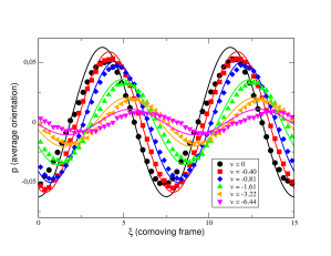
Figure 1: Average orientation of the ABP in the coordinate system which moves with the phase velocity $v$ of the activity wave. Symbols are MD simulations, closed curves are the approximation Eq.  (14). In this example, $n=2$ and $s=1$.

Using Eqs. (10) and (11), the average orientation corresponding to the activity wave in Eq. (7) is obtained as

$$p(z,t)= - \frac{f_{0}\,\omega}{3\zeta}\int_{0}^{\infty}dt^{\prime}\,\int_{-\infty}^{\infty}dz^{\prime}\,\cos\left[\omega(z^{\prime}-v(t-t^{\prime}))\right]$$ (13)

$$\cdot \frac{\exp\left[-2D_{r}t^{\prime}-\frac{(z-z^{\prime})^{2}}{4D_{t}t^{\prime}}\right]}{\sqrt{4\pi D_{t}t^{\prime}}}\;,$$

yielding

$$p(z,t)=-\frac{f_{0}\,\omega\cos\left[\omega(z-vt)+\psi\right]}{3\zeta\sqrt{(2D_{r}+D_{t}\omega^{2})^{2}+v^{2}}}\;,$$ (14)

where we have introduced the phase shift

$$\psi=\arctan\left[\frac{v}{2D_{r}+D_{t}\omega^{2}}\right]\;.$$ (15)

The walker’s orientation, Eq. (14), is stationary in the comoving coordinate frame $\xi=z-vt$ and is shown in Fig. 1: With increasing phase velocity, the amplitude of the orientation is decreasing, while the phase shift increases. This is immediately obvious in Eq. (14), which exhibits the phase velocity in its denominator, and in Eq. (15) in which the phase shift increases linearly with $v$ in its leading order Taylor term. With increasing phase velocity of the activity wave, the activity changes rapidly so that the particle is eventually unable to respond to changes of the external field. The crucial time scale is the rotational relaxation time of $\tau_{r}=1$, and when the activity wave runs from its minimum to its next maximum during that time, the orientation profile is essentially turning flat. This happens at phase velocities of the order of $|v_{\rm max}|\approx\pi/2$. The orientation is generally pointing against the activity gradient, i.e. the ABP is turning toward the direction in which activity decreases sharma_PRE17 .

The linear response theory generally overestimates the degree of orientation, as well as the amount of phase shift. The deviation from the simulation results increases with the magnitude of the driving force, or the pre-factor $f_{0}$ in Eq. (7). On the other hand, we have observed almost perfect agreement with the simulation data when $f_{0}$ was set smaller than 0.1. It is clear that the validity of the linear response approximation remains restricted to the regime of low activities.

IV Density distributions

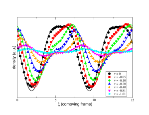
Figure 2: Density distributions of the ABPs in the coordinate comoving frame at different phase velocities of the activity wave. Symbols are MD simulations, closed curves are the approximation Eq.  (20). In this example, $n=2$ and $s=1$.

Traveling activity waves as in Eq. (7) induces traveling orientation waves (Eq. (14)) and traveling density waves. One cannot, however, use linear response approach to calculate the density distribution because it is invariant to activity in the linear order. To calculate density distribution, we integrate over $\bm{p}$, $x$ and $y$ in Eq. (2) to obtain the following 1-dimensional equation for the density $\rho(z,t)$

$$\ \frac{\partial\rho(z,t)}{\partial t}=\frac{\partial}{\partial z}\left[D_{t}\frac{\partial\rho(z,t)}{\partial z}-\frac{f_{0}(z,t)}{\zeta}p(z,t)\rho(z,t)\right].$$ (16)

In the comoving frame $\xi$, Eq. (16) can be recast as a continuity equation

$$\frac{\partial\rho}{\partial t}+\frac{\partial J}{\partial\xi}=0\;,$$ (17)

where $\rho=\rho(z-vt)\equiv\rho(\xi)$ and $J(\xi)$ is the flux in the comoving frame given as

$$J(\xi)=-D_{t}\frac{\partial\rho}{\partial\xi}+\frac{f(\xi)}{\zeta}\,p(\xi)\,\rho(\xi)-v\,\rho(\xi).$$ (18)

Since the density is stationary in the $\xi$-frame, it follows from Eq. (17) that $J(\xi)$ is constant. On integrating Eq. (18) and using periodicity of $p(\xi)$ and $\rho(\xi)$, one obtains the following equations for the flux

$$\frac{J}{\rho_{b}LD_{t}}=\frac{\left[1-\exp\left\{-\int_{0}^{L}\frac{b(z)}{D_{t}}\,dz\right\}\right]}{\int_{0}^{L}dx\,\int_{0}^{L}dy\,\exp\left\{-\int_{x}^{x+y}\frac{b(z)}{D_{t}}\,dz\right\}}\;$$ (19)

and the density

$$\frac{\rho(\xi)}{\rho_{b}}=\frac{L\int_{0}^{L}dy\,\exp\left[-\int_{\xi}^{\xi+y}\frac{b(\xi^{\prime})}{D_{t}}\,d\xi^{\prime}\right]}{\int_{0}^{L}d\xi\,\int_{0}^{L}dy\,\exp\left[-\int_{\xi}^{\xi+y}\frac{b(\xi^{\prime})}{D_{t}}\,d\xi^{\prime}\right],}$$ (20)

with the particle bulk density $\rho_{b}=N/V$ and the function $b(\xi)=\zeta^{-1}f(\xi)\,p(\xi)-v$.

This integral (Eq. (20)) has to be solved numerically, solutions are shown in Fig. 2. We have used the theoretical prediction of Eq. (14) for $p(\xi)$. The linear response theory offers an excellent approximation to the simulation data in the present parameter ranges. Even at high phase velocities, the density distributions are almost quantitatively reproduced. A comparison to Fig. 1 reveals the different time scales at which the variables respond to the activity field: While the density distribution is almost uniform at phase velocities as low as $|v|\approx 1.6$, the polarization pattern is not yet flat at a far higher velocity of $|v|\approx 6.4$. This is a consequence of the longer relaxation times associated with translocations of the ABPs, as compared to their rotational relaxation times. In the present parameter setting, the particle positions relax roughly an order of magnitude slower than their orientations.

V Induced flux

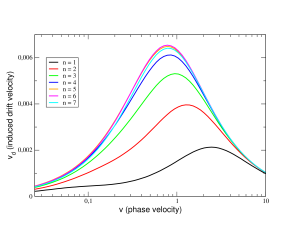
Figure 3: Induced drift velocities (Eq. 21), as a function of the phase velocity of the activity wave. Different curves correspond to different angular frequencies $\omega=2n\pi/L$ that satisfy the periodic boundary condition. Here, the size of the ABP equals $b=1$, the activity factor $f_{0}=2.5$.

The average drift velocity of the ABPs in laboratory frame can be written as

$$v_{d}=\frac{J}{\rho_{b}}+v\;.$$ (21)

Figure 3 displays solutions to Eq. 21 for different angular frequencies $\omega=2n\pi/L$ of the activity waves. As a function of the phase velocity, the induced drift generally exhibits a global maximum, which, however, differs with the angular frequency. The overall maximum value of the drift velocity is found with $n=6$ and a phase velocity about $v\approx 0.75$. We note that an earlier study has reported on situations in which negative drifts, i.e. in the direction opposite to the propagation of the activity wave geiseler_PRE16 ; geiseler_SR17 . So far, we have not been able to reproduce such a phenomenon with our setup in three dimensional systems, neither in linear response approximation nor in simulation. It may well be the case that the parameter range covered in our studies did not allow for such a reversal of the direction of drift.

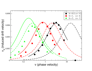
Figure 4: Induced drift velocities as a function of phase velocity for different particle sizes and angular frequencies $\omega=2n\pi/L$. Data points are simulations, solid curves computed from Eq. (21), and dashed curves are the approximation (23).

It is natural to ask how an induced drift would depend upon the properties of the particle. We have repeated the analysis of Fig. 3 with particles of sizes $b=0.5$ and $b=2$, with properties as summarized in Tab. 1. Figure 4 only contains curves for angular frequencies at which the respective particles reach the highest drift velocities. For small ABPs, MD simulations and linear response theory (Eq. (21)) display a reasonably close agreement. For the larger particle of diameter $b=2$ (green curve and triangles), however, significant deviations are visible. Due to their longer rotational relaxation times, the dynamics of these particles are less affected by Brownian motion, i.e. more ballistic, and linear response theory begins to break down. In Sec. VII we are going to discuss the issue of valididy ranges of the linear response approach in detail.

It is instructive to investigate an approximation to the induced drift velocity, considering that the orientation of the particle relaxes faster than its density profile. If the traveling wave propagates sufficiently fast, then $\rho(\xi)$ in Eq. (18) may be approximated by the uniform bulk density, turning Eq. (21) into

$$v_{d}(\xi)\approx\frac{1}{\zeta}p(\xi)\,f(\xi)\;,$$ (22)

which can be integrated over the box to yield the average drift velocity

$$v_{d}=\frac{f_{o}^{2}\omega v}{6\zeta^{2}\left[(2D_{r}+D_{t}\omega^{2})^{2}+v^{2}\right]}\;.$$ (23)

The plots in Fig. 4 show that this approximation (dashed curves) is reasonable only in case of the large particles, which display a sufficiently slow reaction to the incoming activity field so that $\rho(\xi)\approx\rho_{b}$ remains valid. Yet, Eq. (23) provides us with a glimpse of how the underlying dynamics of the ABPs enables the induction of drift: This function has its extremum at

$$\tilde{v}=4D_{r}\sim b^{-3}\;,\;\;\;\;\tilde{\omega}=\sqrt{\frac{2D_{r}}{D_{t}}}\sim b^{-1}\;,$$ (24)

at which it reaches the induced drift velocity of

$$v_{d,\rm max}=\frac{\sqrt{2}}{48}\,\frac{f_{o}^{2}}{\zeta^{2}\sqrt{D_{r}D_{t}}}\sim b^{0}\;,$$ (25)

where we used the fact that $\zeta\sim b$. The optimum choice for the velocity of the traveling wave is determined by the rotational diffusion and thus strongly dependent on the particle size. While the $b^{-3}$-scaling of this approximation to the optimum drift velocity definitely overestimates the simulation results, for which the scaling is closer to $b^{-2}$, the ideal angular frequency is inversely proportional to $b$ in both, approximation and simulation. The peak drift velocity is not an explicit function of the particle size, which is as well supported by the simulations (Fig. 4) and thus no spurious consequence of the uniform-density-approximation. In the laboratory, of course, the driving force $f_{o}$ is likely to depend on the particle diameter and in this way the maximum achievable drift velocities may turn species-dependent.

VI Separation of mixtures of ABPs with different sizes

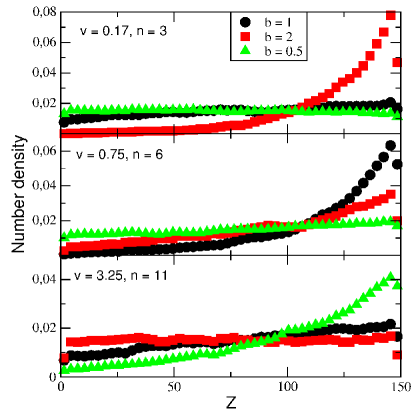
Figure 5: A mixture of three ABP-species of different diameters. Depending on the choices for the phase velocity $v$ and the angular frequency $\omega=2n\pi/L$ of the activity wave, either the large particles (upper panel), the medium sized particles (center panel) or the small particles (lower panel) are enriched near the wall.

In this set of simulations, the box-length was increased to $150$ in z-direction, where the boundaries were fixed with short-range repulsive walls. Three particle species were added, 500 each, with parameters as summarized in Tab. 1. No interactions between particles were enabled, so that these are pure averages of single particle ensembles. Then, activity waves were sent through the system, with positive phase velocities (from the left to the right in Fig. 5) parameters at which the solid curves of Fig. 4, e.g. Eq. (21), had their maxima.

As can be seen in Fig. 4, the different values of induced drift velocities allow for a separation of the mixture of particle species: Either one of the three species may be enriched at the right hand wall, depending on the particular choice of the activity wave. It is therefore possible to separate a mixture of ABPs according to their diameter. In the present simulation, the density distributions of the enriched species had turned stationary after simulation times of roughly $10^{4}$, so that a continuation of that procedure did not improve its selectivity any further.

VII Validity of the linear response approach

The solution to Eq. (2) is based on a separation of the time evolution operator $\Omega_{\rm a}(t)=\Omega_{\rm eq}+\delta\Omega_{\rm a}(t)$ into its (diffusive) equilibrium part and a second, activity driven part, which is treated as a perturbation. This linear response ansatz produces accurate dynamics as long as diffusion dominates over driven motion.

To compare both components, we consider the persistence length of ballistic motion, $l_{b}=v_{b}\tau_{r}=f\tau_{r}/\zeta$, with the average diffusion distance $l_{d}=\sqrt{6D_{t}\tau_{r}}$ during the same time interval $\tau_{r}$. As long as $l_{b}/l_{d}\ll 1$, diffusion dominates the motion. In our present simulations, the peak driving force reaches $f=5$, at which $l_{b}/l_{d}=1/4$ ($b=1/2$), $l_{b}/l_{d}=1/2$ ($b=1$) and $l_{b}/l_{d}=1$ ($b=2$), which indicates that the formalism is likely to break down in case of the large particles, as is obvious in Fig. 4.

A diffusion driven dynamics is not uncommon for ABPs of the sub - $100$ $nm$ scale. As an example, we consider the dynamics of Au-Pt Janus particles of diameter $30$ nm, as prepared and analyzed by Lee et al. lee_NanoLett14 : In a solution of water with 2.5% H₂O₂, these particles developed a considerable ballistic speed of $2.2\cdot 10^{4}$ particle diameters per second. However, due to their small diameters, the rotational diffusion was rapid and allowed for a persistent motion over a distance of only $l_{b}\approx 4.6$ $nm$ during the directional persistence time of $\tau_{r}\approx 7$ $\mu s$. Given the diffusion coefficient of the passive particle, $D_{t}\approx 0.013$ $nm^{2}\cdot ns^{-1}$, the distance of $l_{d}=\sqrt{6D_{t}\tau_{r}}\approx 23$ $nm$ was covered during one persistence time. This yields the ratio $l_{b}/l_{d}\approx 1/5$, so that linear response theory may safely be applied to this system.

We summarize that the linear response approximation describes ABPs at activity levels that are comparable or smaller than the diffusive motion of the particle and may hence be a method of choice for small ABPs of diameters in the sub - $0.1$ $\mu m$ range, as well as for larger particles which are only weakly driven.

VIII Summary

In the present work, a linear response (Green-Kubo) approach has been applied to ABPs that are exposed to time-varying activity fields. We have demonstrated how the distribution of particle orientations, their densities and the resulting induced fluxes are approximated, and shown that these approximations agree closely with Langevin dynamics simulations (Sections III – V).

The accuracy of linear response theory is granted as long as the contribution from their active motion remains weak, so that their diffusive thermal motion is dominating the dynamics. This is naturally the case with small ABPs of sub- 100 $nm$ diameter, or with larger particles that are only weakly driven (Sec. VII).

Dynamic activity waves are capable of inducing fluxes into systems of ABPs, and the efficiency of that coupling is a function of the particle diameter, as is most easily seen in the approximation (24). A tuning of the phase- and angular velocity allows the practitioner to efficiently drive particles of selected diameters through the system, which might be used for a controlled separation of mixtures of ABPs according to their sizes (Sec. VI).

Within the accuracy of the formalism, linear response theory yields the parameters for the activity waves which may be applied to facilitate such a directed transport at highest efficiency.

References

- (1) G. Fenteany and M. Glogauer. Cytoskeletal remodeling in leukocyte function. Curr Opin Hematol., 11:112, 2004.
- (2) Y. Kanai, N. Dohmae, and N. Hirokawa. Kinesin transports rna: isolation and characterization of an rna-transporting granule. Neuron, 43(4):513–525, 2004.
- (3) Howard C. Berg. E. coli in motion. Springer Verlag, Heidelberg, Germany, 2004.
- (4) Stephen J. Ebbens and Jonathan R. Howse. In pursuit of propulsion at the nanoscale. Soft Matter, 6:726–738, 2010.
- (5) Daigo Yamamoto and Akihisa Shioi. Self-propelled nano/micromotors with a chemical reaction: Underlying physics and strategies of motion control. KONA Powder and Particle Journal, 32:2, 2015.
- (6) Loai K. E. A. Abdelmohsen, Fei Peng, Yingfeng Tu, and Daniela A. Wilson. Micro- and nano-motors for biomedical applications. J. Mater. Chem. B, 2:2395–2408, 2014.
- (7) Wei Gao and Joseph Wang. The environmental impact of micro/nanomachines: A review. ACS Nano, 8(4):3170–3180, 2014.
- (8) J. R. Howse, R. A. L. Jones, A. J. Ryan, T. Gough, R. Vafabakhsh, and R. Golestanian. Self-Motile Colloidal Particles: From Directed Propulsion to Random Walk. Physical Review Letters, 99(4):048102, July 2007.
- (9) Wei Gao, Allen Pei, Renfeng Dong, and Joseph Wang. Catalytic iridium-based janus micromotors powered by ultralow levels of chemical fuels. Journal of the American Chemical Society, 136(6):2276–2279, 2014. PMID: 24475997.
- (10) Fei Peng, Yingfeng Tu, Jan C. M. van Hest, and Daniela A. Wilson. Self-guided supramolecular cargo-loaded nanomotors with chemotactic behavior towards cells. Angewandte Chemie, 127(40):11828–11831, 2015.
- (11) Pulak K. Ghosh, Yunyun Li, Fabio Marchesoni, and Franco Nori. Pseudochemotactic drifts of artificial microswimmers. Phys. Rev. E, 92:012114, Jul 2015.
- (12) Hidde Vuijk, Abhinav Sharma, Debasish Mondal, Jens-Uwe Sommer, and Holger Merlitz. Active brownian particles climb up activity gradient to reach the fuel source. submitted to PRL, 2018.
- (13) Celia Lozano, Borge ten Hagen, Hartmut Löwen, and Clemens Bechinger. Phototaxis of synthetic microswimmers in optical landscapes. Nature Communications, 7:12828, 2016.
- (14) Clemens Bechinger, Roberto Di Leonardo, Hartmut Löwen, Charles Reichhardt, Giorgio Volpe, and Giovanni Volpe. Active particles in complex and crowded environments. Reviews of Modern Physics, 88:045006, 2016.
- (15) A. Sharma and J.M. Brader. Communication: Green-kubo approach to the average swim speed in active brownian systems. J. Chem. Phys., 145:161101, 2016.
- (16) A. Sharma and J.M. Brader. Brownian systems with spatially inhomogeneous activity. Phys. Rev. E, 96:032604, 2017.
- (17) Alexander Geiseler, Peter Hänggi, Fabio Marchesoni, Colm Mulhern, and Sergey Savel’ev. Chemotaxis of artificial microswimmers in active density waves. Phys. Rev. E, 94:012613, Jul 2016.
- (18) Alexander Geiseler, Peter Hänggi, and Fabio Marchesoni. Self-polarizing microswimmers in active density waves. Scientific Reports, 7:41884, 2017.
- (19) S.J. Plimpton. Fast parallel algorithms for short-range molecular dynamics. J. Comp. Phys., 117:1, 1995. http://lammps.sandia.gov/.
- (20) Holger Merlitz, Chenxu Wu, and Jens-Uwe Sommer. Directional transport of colloids inside a bath of self-propelling walkers. Soft Matter, 13:3726–3733, 2017.
- (21) C. W. Gardiner. Stochastic Methods of Theoretical Physics, volume 3. Springer, Berlin, 1985.
- (22) Philip McCord Morse, Herman Feshbach, et al. Methods of theoretical physics, volume 1. McGraw-Hill New York, 1953.
- (23) A Sharma and JM Brader. Communication: Green-kubo approach to the average swim speed in active brownian systems. The Journal of Chemical Physics, 145(16):161101, 2016.
- (24) Joseph M Brader, Mike E Cates, and Matthias Fuchs. First-principles constitutive equation for suspension rheology. Physical Review E, 86(2):021403, 2012.
- (25) J.-P. Hansen and I.R. McDonald. Theory of Simple Liquids, volume 3. Elsevier, New York, 1990.
- (26) Tung-Chun Lee, Mariana Alarcon-Correa, Cornelia Mikch, Kersten Hahn, John F. Gibbs, and Peer Fischer. Self-propelling nanomotors in the presence of strong brownian forces. Nano Letters, 14:2407, 2014.