Sample efficient deep reinforcement learning for dialogue systems with large action spaces

Abstract

In spoken dialogue systems, we aim to deploy artificial intelligence to build automated dialogue agents that can converse with humans. A part of this effort is the policy optimisation task, which attempts to find a policy describing how to respond to humans, in the form of a function taking the current state of the dialogue and returning the response of the system. In this paper, we investigate deep reinforcement learning approaches to solve this problem. Particular attention is given to actor-critic methods, off-policy reinforcement learning with experience replay, and various methods aimed at reducing the bias and variance of estimators. When combined, these methods result in the previously proposed ACER algorithm that gave competitive results in gaming environments. These environments however are fully observable and have a relatively small action set so in this paper we examine the application of ACER to dialogue policy optimisation. We show that this method beats the current state-of-the-art in deep learning approaches for spoken dialogue systems. This not only leads to a more sample efficient algorithm that can train faster, but also allows us to apply the algorithm in more difficult environments than before. We thus experiment with learning in a very large action space, which has two orders of magnitude more actions than previously considered. We find that ACER trains significantly faster than the current state-of-the-art.

I Introduction

Traditionally, computers are operated by either a keyboard and a mouse or touch. They provide feedback to the user primarily via visual clues on a display. This human-computer interaction model can be unintuitive to a human user at first, but it allows the user to express its intent clearly, as long as their goal is supported and they are equipped with sufficient knowledge to operate the machine. A spoken dialogue system (SDS)aims to make the human-computer interaction more intuitive by equipping computers with the ability to translate between human and computer language, thereby relieving humans of this burden and creating an intuitive interaction model. More specifically, the objective of an SDS is to help a human user achieve their goal in a specific domain (eg. hotel booking), using speech as the form of communication. Recent advances in artificial intelligence (AI)and reinforcement learning (RL)have established the necessary technology to build the first generation of commercial spoken dialogue system s deployable as regular household items. Examples of such systems are Amazon’s Alexa, Google’s Home or Apple’s Siri. While initially built as voice-command systems, over the years these systems have become capable of sustaining dialogues that can span a few turns.

Spoken dialogue systems are complex as they have to solve many challenging problems at once, under significant uncertainty. They have to recognise spoken language, decode the meaning of natural language, understand the user’s goal while keeping track of the history of a conversation, determine what information to convey to the user, convert that information into natural language, and synthesise the sentences into speech that sounds natural. This work focuses on one particular step in this pipeline: devising a policy that determines the information to convey to the user, given our belief of their goal.

This policy has been traditionally planned out by hand using flow-charts. This was a manual and inflexible process with many drawbacks that ultimately led to systems that were unable to converse intelligently. To overcome this, the policy optimisation problem has been formulated as a reinforcement learning problem [1, 2, 3]. In this formulation, the computer takes actions and gets rewards. An algorithm aims to learn a policy that maximises the rewards through learning to take the best actions based on the state of the dialogue. Since the number of possible states can be very large (potentially infinite), complex and universal function approximators such as neural network s have been deployed as the policy [4, 5, 6]. There is a recent trend in the last years to model text-to-text dialogues with a neural network and tackle it as a sequence to sequence model. Initial attempts to do this underestimate the fact that planning is needed and treat the problem in a purely supervised fashion [7]. More recently RL learning has also been applied yielding improvements [8, 9, 10, 11]. While we focus here on traditional modular approaches, everything that we describe is also applicable to end-to-end modelling.

Using neural network s for policy optimisation is challenging for two reasons. First, there is often little training data available for an SDS as the data often comes from real humans. The system should be able to train quickly in an on-line setting while the training data is being gathered from users, to make the data to be gathered useful. Neural networks often exhibit too much bias or high variance when the volume of training data is small, making it difficult to quickly train them in a stable way. Second, the success or failure of a dialogue may be the only information available to the system to train the policy on. Dialogue success depends crucially on most actions in the dialogue, making it difficult to determine which individual actions contributed to the success, or led to the failure of a dialogue. This problem is exacerbated by the large size of the state space: the system will potentially never be in the same state twice.

We address the above problems in the following ways:

1. We deploy the ACER algorithm [12, 13] which has previously showed promising results on simpler gaming tasks.

2. We analyse the algorithm detail highlighting its theoretical advantages: low variance, safe and efficient learning.

3. We test the algorithm on a dialogue task with delayed rewards and test it alongside state-of-the-art methods in this task

4. After confirming its supremacy on a small action space, we deploy the algorithm on a two orders of magnitude larger action space.

5. We confirm our findings in a human evaluation.

The rest of the paper is organised as follows. First, we give a brief introduction to dialogue management and define the main concepts. Then, in section III we review reinforcement learning. This is followed with an in-depth description of the ACER algorithm in section IV. Then, in section V we describe the architecture deployed to allow the application of ACER to a dialogue problem. The results of the extensive evaluation is given in section VII. In section VIII we give conclusions and future work directions.

II Dialogue management

The job of the dialogue manager is to take the user’s dialogue acts, a semantic representation of the input, and determine the appropriate response also in the format of a dialogue act [14, 15]. The function that chooses the appropriate response is called the policy. The role of dialogue management is two-fold: tracking the dialogue state and optimising the policy.

II-A Belief tracking

We call the user’s overall goal for a dialogue the user goal, i.e. booking a particular flight or finding information about a restaurant. The user works towards this goal in every dialogue turn. In each dialogue turn, the short-term goal of the user is called the user intent. Examples of user intent are: confirm what the system said, inform the system on some criteria, and request more information on something.

The belief tracker is the memory unit of the SDS, with the aim to track the user goal, the user intent and the dialogue history. For the state to satisfy the Markov property it can only depend on the previous state and the action taken. Therefore, the state needs to encode enough information about what happened in the dialogue previously to maintain the conversation. By tracking the dialogue history we ensure that the state satisfies the Markov property. The user intent is derived from the (noisy) dialogue act. To deal with the inherent uncertainty of the input, the dialogue is modelled as a partially observable Markov decision process (POMDP) [3]. The belief state is a vector representing a probability distribution over the different goals, intents and histories that occur in the dialogue. The role of the belief tracker is to accurately estimate this probability distribution and this is normally done using a version of a recurrent neural neural network [16].

II-B Policy optimisation

A policy is a probability distribution over possible user actions given the current belief state, and is commonly written as $P_{\pi}(a|b)=\pi(a|b)$. Here, $a$ is the action and $b$ is the output of the belief tracker, which is interpreted as a vector of probabilities.

In order to define the optimal policy, we need to introduce a utility function (reward) that describes how good taking action $a$ is in state $b$. The reward for a complete dialogue depends on whether the user was successful in reaching their goal and the length of the conversation, such that short successful dialogues are preferred. Thus, the last dialogue interaction gains a reward based on whether the dialogue was successful, and every other interaction loses a small constant reward, penalising for the length of the dialogue. The task of policy optimisation is to maximise the expected cumulative reward in any state $b$ when following policy $\pi$, by choosing the optimal action $a$ from the set of possible actions $\mathbb{A}$. Finding the optimal policy is computationally prohibitive even for very simple POMDPs. We can view the partially observable Markov decision process (POMDP)as a continuous-space Markov decision process (MDP)in terms of policy optimisation, where the states are the belief states [17]. This allows us to apply function approximation to solve the problem of policy optimisation. This is the approach we adopt in this work.

II-C Action spaces

System actions are the dialogue acts that the system can give as a response. This is called the action space or the master action space. Due to its large size, training a dialogue policy in this action space is difficult. Some algorithms do not converge to the optimal policy, converge very slowly, or, in rare cases, have prohibitive computational demands.

To alleviate this problem, we use the summary action space which contains a much smaller number of actions. If a policy is trained on the summary action space, the action selected by the policy needs to be converted to a master action. The conversion is a set of heuristics that attempts to find the optimal slots to inform on given the belief state.

Using the summary action space provides the clear benefit of a simpler dialogue policy optimisation task. On the other hand, the necessary heuristics to map to the master action space need to be manually constructed for each domain. This means that the belief state needs to be human interpretable. This limits the applicability of neural networks for belief tracking where the belief state is compactly represented as a hidden layer in the neural network.

The description of the summary and master actions that we consider is given in Appendix A.

II-D Execution mask

Not every system action is appropriate in every situation (belief state). For example, inform is not a valid action at the very beginning of the dialogue, when the system has not yet received any information on what kind of entity the user is looking for. An execution mask is constructed by the designer that ensures that only valid actions are selected by the policy: the probability of invalid actions is set to zero. The execution mask depends on the current belief state. Note that removing this mask inherently complicates the task of policy learning, as the policy then has to learn not to select inappropriate actions based on the belief state.

III Reinforcement learning

In reinforcement learning, an agent interacts with the environment in discrete time steps. In each time step, the agent observes the environment as a belief state vector $b_{t}$ and chooses an action $a_{t}$ from the action space $\mathbb{A}$. After performing action $a_{t}$, the agent observes a reward $r_{t}$ produced by the environment.

The cumulative discounted return is the future value of an episode of interactions. For the $t^{\text{th}}$ timestep, we calculate this as

$$R_{t}=\sum_{i\geq 0}\gamma^{i}r_{t+i}.$$

The discount factor $\gamma$ trades-off the importance of immediate and future rewards. The goal of the agent is to find a policy that maximises the expected discounted cumulative return for every state. We define the value of a state-action pair $(b_{t},a_{t})$ under policy $\pi$ to be the Q-value function, the expectation of the return for belief state $b_{t}$ and action $a_{t}$:

$$Q_{\pi}(b_{t},a_{t})=\mathop{\mathbb{E}_{\pi}}\big{(}R_{t}|b_{t},a_{t}\big{)},$$

and the value of a state $b_{t}$ is the value function, which is the expected return only conditioned on the belief state $b_{t}$:

$$V_{\pi}(b_{t})=\mathop{\mathbb{E}}_{\pi}\big{(}R_{t}|b_{t}\big{)}.$$

In both definitions, the expectation is taken over the states the environment could be in after performing the current action, and the future actions selected by policy $\pi$ [18].

As the reinforcement learning scenarios become more challenging, the agent estimates value functions from trial and error by interacting with a simulated or real environment. These estimates are accurate only in the limit of infinite observations for each state-action pair, thus a requirement for the behaviour policy $\mu$ is to maintain exploration, i.e. to keep visiting all state-action pairs with non-zero probability. The behaviour policy is the policy used to generate the data during learning. For on-policy methods, the behaviour policy is the same as the learned policy $\pi$, in other words, we evaluate and improve the same policy that is used to make decisions. In contrast, off-policy methods evaluate and improve a policy different from the one used to generate the data, i.e. the behaviour policy and the learned policy can be different. The advantage of off-policy methods is that the optimal policy can be even while we are choosing sub-optimal actions according to the behaviour policy.

Standard reinforcement learning algorithms require that the state space is discrete. Therefore, the belief state of a dialogue manager is often discretised to allow standard algorithms to be applied [19]. Alternatively, function approximation can be applied for $Q$, $V$ or $\pi$. In [20], linear function approximation was applied to value functions. As parametric function approximation can limit the optimality of the solution, GP-SARSA [21] instead models the Q-function as a Gaussian process. The key here is the kernel function which models the correlation between different states and allows uncertainty to be estimated. This is crucial for learning from a small number of samples. More recently, neural network function approximation was used to approximate the Q-value function, known as deep Q-learning (DQN), obtaining human-level performance across challenging video games [22]. The policy $\pi$ can be also modelled directly by deep networks leading to the resurgence of actor-critic methods [23]. The actor is improving its policy $\pi$ through interactions being directed by the critic (value function $V$).

III-A Neural networks in dialogue management

A number of deep learning algorithms were previously applied to dialogue management. It has been shown in [24] that DQN enables learning strategic agents with negotiation abilities operating on a high-dimensional state space. The performance of actor-critic models on task-oriented dialogue systems was analysed in [6]. These models can also be naturally bootstrapped with a small number of dialogues via supervised pre-training. They reported superior performance compared to GP-SARSA in a noise-free environment. However, the compared GP-SARSA did not utilise uncertainty estimates which were previously found to be crucial for effective learning [21].

Uncertainty estimates can be incorporated into DQN using Bayes-by-Backprop [25]. Initial results show an improvement in learning efficiency compared to vanilla DQN.

A number of recent works investigated end-to-end using gradient descent techniques [26, 27, 7], where belief tracking and policy optimisation are optimised jointly. While, end-to-end modelling goes beyond the scope of this work, we note that the presented algorithm is applicable also in that setting.

IV ACER

This paper builds on recent breakthroughs in deep reinforcement learning (DRL)and applies them to the problem of dialogue management. In particular, we investigate recently proposed improvements to the actor-critic method [12]. The goal is a stable and sample efficient learning algorithm that performs well on challenging policy optimisation tasks in the SDS domain. Recent advances in DRL apply several methods, including experience replay [28], truncated importance sampling with bias correction [12], the off-policy Retrace algorithm [13] and trust region policy optimisation [23] to various challenging problems. The core of this paper is to investigate to what extent these advances are applicable to the dialogue policy optimisation task with a large action space. These methods were recently combined in the actor critic with experience replay (ACER)algorithm and tested in gaming environments. To this end, we explain actor critic with experience replay (ACER)in detail and investigate the steps needed to apply it to SDS. Unlike in games, where these methods have been previously applied, we investigate dialogues with large and uncertain belief states and very large action spaces. This necessitates function approximation in reinforcement learning, but previously examined methods in SDS are data-inefficient, unstable or computationally too expensive. We investigate ACER as a means to overcome these limitations.

IV-A Actor-critic with Experience Replay

In order to use experience replay in an actor-critic method, an off-policy version of the actor-critic method is needed. The objective is to find a policy that maximises the expected discounted return. This is equivalent to maximising the value of the initial state with input parameter vector $\omega$:

$$J(\omega)=V_{\pi(\omega)}(b_{0}).$$

Another way of expressing the same objective is to maximise the cumulative reward received from the average state [29]. For behaviour policy $\mu$, let the occupancy frequency $d^{\mu}$ be defined as:

$$d^{\mu}(b)=\lim_{t\to\infty}P(b_{t}=b|b_{0},\mu).$$

According to the new definition of $J(\omega)$, $V$ is weighted by $d^{\mu}$ because $\mu$ was used to collect the experience:

$$J(\omega)=\sum_{b\in\mathbb{B}}d^{\mu}(b)V_{\pi(\omega)}(b),$$

where $\pi$ is the optimal policy.

The off-policy version of the Policy Gradient Theorem [30] is used to derive the gradients $\nabla_{\omega}J(\omega)\approx g(\omega)$:

$$g(\omega)=\sum_{b\in\mathbb{B}}d^{\mu}(b)\sum_{a\in\mathbb{A}}\nabla_{\omega}\pi(a|b)Q_{\pi}(b,a)$$ (1)

The states are encountered in proportions according to $d^{\mu}$ just by sampling from the experience memory, so there is no need to estimate $d^{\mu}$ explicitly. Estimating $Q_{\pi}$, however, is more difficult: the off-policy interactions are gathered according to $\mu$, and we need the $Q$-function under a different - current policy $\pi$.

To account for this, the importance sampling (IS)weights [31] could be used. To achieve stable learning, we use an estimation method that achieves low variance by considering state-action pairs in isolation, applying only one IS weight for each.

Continuing from Equation (1), the approximation of the true gradient can be derived:

$$g(\omega) =\mathop{\mathbb{E}}\left[\sum_{a\in\mathbb{A}}\nabla_{\omega}\pi(a|b)Q_{\pi}(b,a)|b\sim d^{\mu}\right]$$

$$=\mathop{\mathbb{E}}\left[\sum_{a\in\mathbb{A}}\mu(a|b)\frac{\pi(a|b)}{\mu(a|b)}\frac{\nabla_{\omega}\pi(a|b)}{\pi(a|b)}Q_{\pi}(b,a)|b\sim d^{\mu}\right]$$

$$=\mathop{\mathbb{E}}\left[\rho(a|b)\nabla_{\omega}\log\pi(a|b)Q_{\pi}(b,a)|b\sim d^{\mu},a\sim\mu(\cdot|b)\right],$$

where $\rho(a|b)=\frac{\pi(a|b)}{\mu(a|b)}$ are the importance sampling (IS)weights. The advantage function $A_{\theta}$ is used in place of the $Q$-function for an unbiased estimate with a lower variance:

$$g(\omega)=\mathop{\mathbb{E}}_{\mu}\left[\rho(a|b)\nabla_{\omega}\log\pi(a|b)A_{\theta}\right].$$

In off-policy setting, the advantage function is approximated as as $r_{t}+\gamma V(b_{t+1},\theta)-V(b_{t},\theta)$.

IV-B Lambda returns

The unbiased estimator

$$Q_{\pi}(b_{t},a_{t})\approx\sum_{i=t}^{T}\gamma^{i}r_{i}$$

results in high variance, due to the IS weight that has to be calculated for the entire episode. The temporal difference (TD)estimation

$$Q_{\pi}(b_{t},a_{t})\approx r_{t}+\gamma V(b_{t+1},\theta)$$ (2)

only requires a single IS weight. However, this estimation is biased: the value function update of the current state is based on the current estimate of the value function for the next state. This leads to slow convergence or no convergence at all.

It is possible to combine both methods and create an estimator that trades off bias and variance according to a parameter $\lambda$. [29] estimate $Q_{\pi}$ as:

$$Q_{\pi}(b_{t},a_{t})\approx R_{t,\lambda}\mbox{, where}$$

$$R_{T,\lambda} =r_{T}$$

$$R_{t,\lambda} =r_{t}+(1-\lambda)\gamma V(b_{t+1})+\lambda\gamma\rho_{t+1}R_{t+1,\lambda}.$$

The constant $\lambda$ controls the bias-variance trade-off: setting $\lambda$ to 0 results in an equivalent estimation as in Equation (2), with a low variance but high bias. Conversely, setting $\lambda$ to 1 results in high variance as many IS weights will be producted. This has the advantage of propagating the final reward further to the starting state which reduces bias.

IV-C Retrace

The Retrace algorithm ([13]) attempts to estimate the current $Q$-function from off-policy interactions in a safe and efficient way, with small variance. Throughout this discussion, we call a method safe if its estimate of $Q^{\pi}$ can be proven to converge to $Q^{\pi}$. The updated estimate of the $Q$-function, $Q^{ret}$ is computed based on state-action trajectories sampled from the replay memory:

$$Q^{ret}(b,a)=Q(b,a)+$$

$$\mathop{\mathbb{E}}_{\mu}\left[\sum_{t\geq 0}\gamma^{t}\left(\prod_{s=1}^{t}c_{s}\right)(r_{t}+\gamma V(b_{t+1})-Q(b_{t},a_{t}))\right].$$ (3)

The methods that stem from this framework differ only in their definition of eligibility traces $c_{s}$.

This framework introduces changes to the actor-critic model. Instead of approximating $V$ and $\pi$ with NN s and estimating $Q$ in a closed-form equation to compute the update targets, both $\pi$ and $Q$ are estimated with NN s. $V$ is then computed from $\pi$ and $Q$:

$$V(b)=\mathop{\mathbb{E}}_{\pi}\left[Q(b,\cdot)\right]=\sum_{a}\pi(a|b)Q(b,a).$$ (4)

We focus on Retrace proposed by [13] where $c_{s}=\lambda\min\left(1,\rho(a_{s}|b_{s})\right)$. Ideally, we need a method that is safe, has low variance and is as efficient as possible. Retrace solves this trade-off by setting the traces “dynamically”, based on the IS weights. In the near on-policy case, it is efficient as IS weights will be about 1, preventing the traces from vanishing. It has low variance because the IS weights are clipped at 1. It is also safe for any $\pi$ and $\mu$. The goal of this discussion is limited to conveying the intuition behind Retrace, but a full proof of safety is available in [13].

IV-D Computational cost

Let us investigate the computational cost of deriving $Q^{ret}$ from $Q$ in a naïve way. For each episode sampled from the replay memory, and for each state-action pair, we need to visit the remaining part of the episode to calculate the expectation of errors under $\mu$ according to Equation (3). This quadratic element of the computational cost can be reduced to a linear one by deriving $Q^{ret}$ in a recursive way. For an episode trajectory $b_{1:T},a_{1:T}$ sampled from the replay memory, Equation (3) becomes:

$$Q^{ret}(b_{i},a_{i}) =r_{i}+\gamma V(b_{i+1})$$

$$\quad\;+\gamma c_{i+1}\left(Q^{ret}(b_{i+1},a_{i+1})-Q(b_{i+1},a_{i+1})\right).$$

We will use this more computationally efficient, recursive formulation of $Q^{ret}$.

IV-E Importance weight truncation with bias correction

Currently, we calculate the policy gradient as:

$$g(\omega)=\mathop{\mathbb{E}}_{b_{t}\sim d^{\mu},a_{t}\sim\mu}\left[\rho(a_{t}|b_{t})\nabla_{\omega}\log\pi(a_{t}|b_{t})A_{\pi}(b_{t},a_{t})\right],$$ (5)

where the expectation is taken over the replay memory, and $\rho(a_{t}|b_{t})=\frac{\pi(a_{t}|s_{t})}{\mu(a_{t}|s_{t})}$. An issue with this approximation is that the IS weights $\rho(a_{t}|b_{t})$ are potentially unbounded, introducing significant variance. To solve this problem, we clip the IS weights from above by a constant $c$: $\overline{\rho}(a_{t}|b_{t})=\min\{c,\rho((a_{t}|b_{t}))\}$. We can split the equation into two parts, one involving the truncated IS weight, and the other the residual. We also need to estimate the residual, otherwise we introduce bias in the gradient estimation. We call the residual the bias correction term.

$$g(\omega) =\mathop{\mathbb{E}}_{b_{t}\sim d^{\mu}}\Big{[}\mathop{\mathbb{E}}_{a_{t}\sim\mu}\overline{\rho}(a_{t}|b_{t})\nabla_{\omega}\log\pi(a_{t}|b_{t})A_{\pi}(b_{t},a_{t})$$

$$\quad+\mathop{\mathbb{E}}_{a_{t}\sim\mu}\left[\rho(a_{t}|b_{t})-c\right]_{+}\nabla_{\omega}\log\pi(a_{t}|b_{t})A_{\pi}(b_{t},a_{t})\Big{]},$$

where $[\cdot]_{+}=\max(0,\cdot)$. The weight of the bias correction term, $\left[\rho(a_{t}|b_{t})-c\right]_{+}$, can still be unboundedly large. This can be solved by sampling the action from the distribution $\pi$ rather than $\mu$ [12]:

$$\begin{split}g(\omega)&=\mathop{\mathbb{E}}_{b_{t}\sim d^{\mu}}\Bigg{[}\mathop{\mathbb{E}}_{a_{t}\sim\mu}\overline{\rho}(a_{t}|b_{t})\nabla_{\omega}\log\pi(a_{t}|b_{t})A_{\pi}(b_{t},a_{t})\\ &\quad\quad+\mathop{\mathbb{E}}_{a\sim\pi}\left[\frac{\rho(a|b_{t})-c}{\rho(a|b_{t})}\right]_{+}\nabla_{\omega}\log\pi(a|b_{t})A_{\pi}(b_{t},a)\Bigg{]}.\end{split}$$ (6)

There are two key advantages of this formulation:

• The bias correction term ensures that the estimate of the gradient remains unbiased.

• The bias correction term is only active when $\rho(a|b)>c$, and otherwise the formulation is equivalent to Equation (5). When active, the bias correction weight falls between 0 and 1.

To apply this method, called the truncation with bias correction trick by [12], we have to overcome a problem with the advantage function estimation. Before, we estimated $A_{\pi}(b,a)=Q^{ret}(b,a)-V(b)=Q^{ret}(b,a)-\sum_{a}\pi(a|b)Q(b,a)$ for belief-action pairs that we sampled from the replay memory, Equation (4). For the bias correction term however, only the belief is sampled from the memory, and all the actions are considered and weighted by the current policy $\pi$. Due to the way $Q^{ret}$ is formulated, it learns from rewards, and only learns belief-action pairs that have been visited and sampled from the replay memory. Thus the estimation is not available for the bias correction term, so we use the output of the NN, $Q$, to estimate the advantage function for that term: $A^{\prime}_{\pi}(b,a)=Q(b,a)-\sum_{a}\pi(a|b)Q(b,a)$.

IV-F Trust Region Policy Optimisation

Typically, the step size parameter in the gradient descent is calculated assuming the that the policy parameter space is Euclidian. However, this has a major shortcoming: small changes in the parameter space can lead to erratic changes in the output policy [32, 33]. This could lead to unstable learning or a learning rate too small for quick convergence. This is solved in the Natural Actor Critic algorithm by considering the natural gradient [34].

Instead of computing the exact natural gradient, we can approximate it. For the natural gradient, the distance metric tensor is the Fisher information matrix:

$$(G_{\omega})_{ij}=\mathop{\mathbb{E}}\left[\frac{\delta\log p(x|\omega)}{\delta\omega_{i}}\frac{\delta\log p(x|\omega)}{\delta\omega_{j}}\right].$$

It can be shown [35] that

$$d\omega^{T}G_{\omega}d\omega\approx\mbox{KL}(\pi(\cdot|b,\omega)||\pi(\cdot|b,\omega+d\omega)),$$

Where KL is the Kullback-Leibler divergence. Thus, instead of directly restricting the learning step-size with the natural gradient method, we can approximate the same method by restricting the Kullback-Leibler divergence between the current policy $\pi$ parametrised by $\omega$, and the updated policy parametrised by $\omega+\alpha\cdot\nabla_{\omega}J$, for learning rate $\alpha$. This method is called trust region policy optimisation (TRPO), introduced by [23]. Their method, however, relies on repeated computations of Fisher matrices for each update, which can be prohibitively expensive. [12] introduces an efficient TRPO method that we will adopt instead. Our description of the method largely follows theirs with additional explanations and necessary adaptation to our discrete action-space SDS domain.

To begin with, [12] proposes that the KL-divergence to the updated policy should be measured not from the current policy, but from a separate average policy instead. This stabilises the algorithm by preventing it from gaining momentum in a specific direction. Instead, it is restricted to stay around a more stable average policy $\pi_{a}$. The average policy is parametrised with $\omega_{a}$, where $\omega_{a}$ represents a running average of all previous policy parameters. It is updated softly after each learning step as:

$$\omega_{a}\leftarrow\beta\omega_{a}+(1-\beta)\omega.$$

$\beta$ is a hyperparameter that controls the amount of history to maintain in the average policy. A value close to zero makes the average policy forget the history very quickly, reducing the effect of calculating the distances from the average policy instead of the current one. A value close to one will prevent the average policy to adjust to the current policy, or slows this adjustment process down.

TRPO can be formulated as an optimisation problem, where we aim to find $z$ that minimises the L2-distance between $z$ and the vanilla gradient $g(\omega)$ from 6. This is a quadratic minimisation. In addition, our aim is for the divergence constraint to be formulated in a linear way, which will allow to derive a closed-form solution. Since $z$ will be used for the parameter update, we have $\omega^{\prime}=\omega+\alpha z$, where $\omega^{\prime}$ denotes the updated parameter vector. We can approximate the KL divergence after the policy update using a first-order Taylor expansion:

$$\mbox{KL}\left[\pi(\cdot|\omega_{a})||\pi(\cdot|\omega^{\prime})\right]=$$

$$\mbox{KL}\left[\pi(\cdot|\omega_{a})||\pi(\cdot|\omega)\right]+\nabla_{\omega}\mbox{KL}\left[\pi(\cdot|\omega_{a})||\pi(\cdot|\omega)\right]^{T}\cdot\alpha z.$$

So the increase in KL divergence in this step is

$$\nabla_{\omega}\mbox{KL}\left[\pi(\cdot|\omega_{a})||\pi(\cdot|\omega)\right]^{T}\cdot\alpha z.$$

We can constrain this increase to be small by setting $\delta$, such that

$$\nabla_{\omega}\mbox{KL}\left[\pi(\cdot|\omega_{a})||\pi(\cdot|\omega)\right]^{T}\cdot z\leq\delta,$$

where the learning rate $\alpha$ is left out, since it is a constant and can be incorporated into $\delta$. Letting $k=\nabla_{\omega}\mbox{KL}\left[\pi(\cdot|\omega_{a})||\pi(\cdot|\omega)\right]$, the optimisation problem with linearised KL divergence constrain is [12]:

$$\underset{z}{\text{minimize}} \frac{1}{2}||g(\omega)-z||^{2}_{2}$$

subject to $$k^{T}z\leq\delta$$

Since the constraint is linear, the overall optimisation problem reduces to a simple quadratic programming problem. Thus, a closed-form solution can be derived using the KKT conditions [36]:

$$z=g-\max\{0,\frac{k^{T}g-\delta}{||k||_{2}^{2}}k\}.$$

IV-G Summary of ACER

ACER is the result of all methods presented in this section. With on-policy exploration, it is a modified version of A2C. Both ACER and A2C use experience replay and sample from their memories to achieve high sample efficiency. The difference between them is that ACER additionally employs TRPO, and that it uses a $Q$-function estimator instead of a $V$-function estimator as the critic. When off-policy, it uses truncated importance sampling with bias correction [12] to reduce the variance of IS weights without adding bias. The Retrace algorithm is used to compute the targets based on the observed rewards in a safe, efficient way, with low bias and variance.

This training algorithm is presented in pseudocode (Algorithm 2), and is called from the master ACER algorithm (Algorithm 1). It performs $\epsilon$-greedy exploration, i.e. the optimal action learned so far with probability $1-\epsilon$, and a random action with probability $\epsilon$. A hyperparameter batch_size controls the number of dialogues considered for a training step, and $n$ controls the number of training steps for each new dialogue gathered. We will investigate the effect of various hyperparameters and how to set them in Section VII-E.

Algorithm 1 ACER master algorithm

1:Input: policy $\pi(a|b,\omega)$, $Q_{\theta}(b,a)$, hyperparameters $\alpha,\beta,\gamma,\delta$

2:Initialise $\theta,\omega,\omega_{a}$, and $Q_{\theta}(\mbox{terminal})=0$

3:repeat

4:     Generate episode $\{b_{0:T},a_{0:T},r_{0:T}\}$ according to $\epsilon$-greedy using $\pi(\cdot|\cdot,\omega)$

5:     Save generated episode, along with values of $\pi(\cdot|\cdot,\omega)$

6:     for $i=1$ to $n$ do

7:         Sample a subset of replay memory, $M$, of size batch_size

8:         Call training algorithm (Algorithm 2) with $\{M,\theta,\omega,\omega_{a},\pi,Q,\alpha,\beta,\gamma,\delta\}$      

9:until convergence

Algorithm 2 ACER training algorithm

1:Input: $\{M,\theta,\omega,\omega_{a},\pi,Q,\alpha,\beta,\gamma,\delta\}$

2:Initialise $g=0,\;d\theta=0$

3:for each dialogue $\{b_{1:N},a_{1:N},r_{1:N},\mu\}$ in M do

4:     for $1=N$ to $1$ do

5:         $\rho_{t}\leftarrow\frac{\pi(a_{t}|b_{t},\omega)}{\mu(a_{t}|b_{t})}$

6:         $V(b_{t})\leftarrow\sum_{a}Q_{\theta}(b_{t},a)\pi(a|b_{t},\omega)$

7:         $Q^{ret}\leftarrow r_{t}+\gamma Q^{ret}$

8:         $A_{\pi}(b_{t},a_{t})\leftarrow Q^{ret}-V(b_{t})$

9:         $A^{\prime}_{\pi}(b_{t},a_{t})\leftarrow Q_{\theta}(b_{t},a_{t})-V(b_{t})$

10:         $\overline{\rho}_{t}\leftarrow min(r,\rho_{t})$

11:         $C\leftarrow\left[\frac{\rho(a|b_{t},\omega)-c}{\rho(a|b_{t},\omega)}\right]_{+}$

12:         $B\leftarrow\sum_{a}\pi(a|b_{t},\omega)\>C\>\nabla_{\omega}\log\pi(a|b_{t},\omega)A^{\prime}_{\pi}(b_{t},a)$

13:         $g\leftarrow g+\overline{\rho}_{t}\nabla_{\omega}\log\pi(a_{t}|b_{t},\omega)A_{\pi}(b_{t},a_{t})+B$

14:         $d\theta\leftarrow d\theta-\nabla_{\theta}(Q^{ret}-Q_{\theta}(b_{t},a_{t}))^{2}$

15:         $Q^{ret}\leftarrow\overline{\rho}_{t}(Q^{ret}-Q_{\theta}(b_{t},a))+V(b_{t})$      

16:$k\leftarrow\nabla_{\omega}\mbox{KL}\left[\pi(\cdot|\omega_{a})||\pi(\cdot|\omega)\right]$

17:$z\leftarrow g-\max\{0,\frac{k^{T}g-\delta}{||k||_{2}^{2}}k\}$

18:$\omega\leftarrow\omega+\alpha\cdot z$

19:$\theta\leftarrow\theta+\alpha\cdot d\theta$

20:$\omega_{a}\leftarrow\beta\omega_{a}+(1-\beta)\omega$

V ACER for dialogue modelling

In this section we detail the steps needed to apply ACER to a dialogue task.

V-A Learning in summary action space

Let us design the neural network s for actor-critic for a dialogue management task. On top of the input of the belief state, we build two hidden layers, $h_{1}$ and $h_{2}$. The heads of the NN are the functions $\pi$ and $Q$. Both hidden layers $h_{1}$ and $h_{2}$ are shared between the predictors of $Q$ and $\pi$. Weight sharing can be beneficial as it reduces the number of parameters to train. Furthermore, in a dialogue system, we expect a strong positive correlation between $\pi$ and $Q$. The architecture is illustrated in Figure 1.

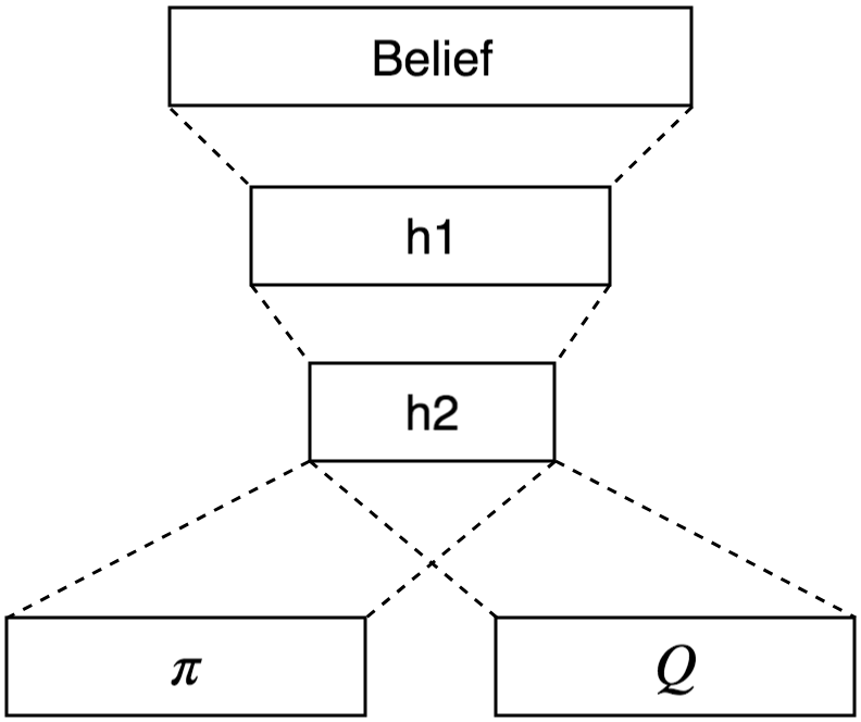
Figure 1: ACER neural network architecture for dialogue management.

The activation function for layers $h_{1}$ and $h_{2}$ is rectified linear unit (ReLU), which was chosen empirically as it led to faster training. The activation function for $\pi$ is softmax, which converts the inputs to a probability distribution with values between 0 and 1, summing up to 1. There is no activation function for the output $Q$, as we want it to have an unlimited range, both from above and below (as rewards can be negative). All the connections in the NN are fully connected, which imposes the least structural constraints on the architecture. We perform our experiments on the Cambridge Restaurants domain, the details of which are given in Appendix A. In this domain the belief state is represented by a 268-dimensional vector. This is the input of the NN. Our layer $h_{1}$ consists of 130 neurons and $h_{2}$ has 50 neurons. These numbers were chosen empirically, with the goal in mind to force the NN to encode all information about the belief state relevant to $\pi$ and $Q$ in the bottleneck layer of 50 neurons, thereby learning a mapping that generalises better. The output vectors $\pi$ and $Q$ have the dimensionality of the action space. Initially, we experiment with the summary action space, which has 15 actions (see Appendix A for details).

V-B Learning in master action space

V-B1 Master actions for ACER

In addition to applying ACER on the summary space, we also applied it on the master action space. However, to make this efficient, the NN architecture was redesigned.

In the case of the CamInfo domain (see Appendix A), there are 8 informable slots of an entity, each with a binary choice on whether we inform on it. Thus, a single inform action makes up $2^{8}=256$ separate master actions, only differing in what they inform on. We want to incorporate the fact that these actions are very similar into the design of the NN architecture. We achieve this by breaking the policy $\pi$ into a summary policy $\pi_{s}$, corresponding to the 15-dimensional summary action space, and a payload policy $\pi_{p}$, corresponding to the $256$ choices of the payload of an inform action. We break the $Q$ function up similarly into $Q_{s}$ and $Q_{p}$. We reconstruct the 1035-dimensional master policy $\pi$ (see Appendix A). and master $Q$-function $Q$ as follows: for each summary action $A$,

• If $A$ does not have a payload (i.e. is not an inform action), append the corresponding summary values from $\pi_{s}$ and $Q_{s}$ onto $\pi$ and $Q$.

• Otherwise, for each payload $P$ of the $256$ possible choices, append $\pi_{s}(A)\cdot\pi_{p}(P)$ to $\pi$. This is because the probability of choosing action $A$ with payload $P$ is modelled as the product of the probability of choosing $A$ and that of choosing $P$. For each $P$, we also append $Q_{s}(A)+Q_{p}(P)$ to $Q$, allowing the payload network to learn an offset of $Q$ achieved by choosing a particular payload.

The complete NN architecture is illustrated in Figure 2. It is important to note that only the architecture of the NN s is changed and the training algorithm is unchanged. In fact, the NN s are treated as a black box by ACER. These output is a 1035-dimensional vector for master action space.

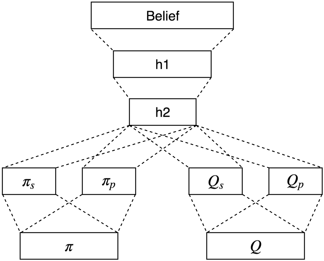
Figure 2: Architecture of the actor-critic neural network for the master action space.

V-B2 Master actions for GP-SARSA

We compare ACER to GP-SARSA algorithm. This is an on policy algorithm that approximates the $Q$-function as a Gaussian process (GP) and therefore is very sample-efficient [21]. The key is the use of a kernel function which defines correlations between different parts of the input space. Similarly to ACER, the Gaussian process (GP) method needs to be adjusted before we deploy it on master action space. The core of a GP is the kernel function, which in the case of GP-SARSA is defined as:

$$k((b,a),(b^{\prime},a^{\prime}))=\langle b,b^{\prime}\rangle\delta(a,a^{\prime}).$$

We recall that the kernel function defines our a priori belief of the covariance between any two belief-action pairs. This kernel is a multiplication of a scalar product of the beliefs and a Kronecker delta on the actions. The latter has the effect that any two different actions are considered completely independent. While this might be a good approximation for summary actions, a more elaborate action kernel is required for master actions. This could introduce the idea that two inform actions with slightly different payloads are expected to have similar results on the same belief state, thus showing higher covariance.

Our new action kernel returns $0$ for actions $a$ and $a^{\prime}$ that stem from different summary actions. Otherwise, $a$ and $a^{\prime}$ are the same inform action with differing payloads. In this case, we calculate the kernel based on the cosine similarity of the two payloads, treating the payloads as vectors describing the sets of slots to inform on. Let us call $a^{s}$ and $a^{p}$ the summary action and the payload corresponding to $a$. $a^{p}$ is represented as a vector where each entry is either $0$ or $1$, depending on whether the corresponding slot is informed on. Writing $\overline{a^{p}}=\frac{a^{p}}{||a^{p}||^{\frac{1}{2}}}$ for the normalised version of the payload vector, the kernel becomes $k((b,a),(b^{\prime},a^{\prime}))=\langle b,b^{\prime}\rangle\delta(a^{s},a^{\prime s})\langle\overline{a^{p}},\overline{a^{\prime p}}\rangle$. Refer to [36] for a proof of $k$ being a valid kernel function.

In the case of GP-SARSA on master action space, the training algorithm is unchanged. Only the kernel function is adjusted to incorporate the idea of similarity between master actions. The GP can thus be trained on the 1035-dimensional master action space.

VI Limitations

It is important to highlight some limitations of this work. This work is not addressing the problem of modelling policy with large action space where there are no similarities between the system actions. On the contrary, we focus on large action spaces where we can establish some relations between the actions, either by sharing the weights in the neural network architecture as in Section V-B1 or by defining special kernel functions as in Section V-B2. Although, this might seem limiting, in practice, in any task-oriented dialogue, actions will bear a lot of similarities. This used to be addressed by producing a smaller summary space of distinct actions, but we believe that the proposed approach scales better, removes hand-crafting and leads to the better performance. The latter hypothesis is investigated in the next section.

VII Evaluation

In this section, we evaluate the performance of ACER incorporated in an SDS. We find that ACER delivers the best performance and fastest convergence among the compared NN-based algorithms (eNAC and A2C) implemented in the PyDial dialogue toolkit [37]. We also deploy the algorithm in a more challenging setting without the execution mask aiding action selection. Next, we investigate the effect of different hyperparameter selections, and the algorithm’s stability against it. Then, we deploy ACER and GP on master action space. Finally, we investigate how resilient different algorithms are to semantic errors and changing testing conditions.

VII-A Evaluation set-up

We compare our implementation of ACER two NN-based algorithms, namely eNAC ([38]) and A2C and to a non-parametric algorithm GP.

Experiments are run as follows. First, the total number of dialogues or iterations ($4000$) is broken down into milestones ($20$ milestones of $200$ iterations each). As the training over the total number of iterations progresses, a snapshot of the state of the training (all NN weights, hyperparameters, and replay memory) is saved at each milestone. A separate run of 4000 iterations is then performed without any training steps, where each of the saved snapshots are tested for 200 iterations. No training and no exploration is being performed during the testing phase; instead of $\epsilon$-greedy, the greedy policy with respect to $\pi$ is used to derive the next action. This informs us on the performance of the system as if it stopped training at a specific milestone, allowing us to observe the speed of convergence and the performance of early milestones, discounting for the exploration.

We run the evaluation $15$ times and average the results, to reduce the variance arising from different random initialisations. We compare the average per-episode reward obtained by the agent, the average number of turns in a dialogue and the percentage of successful dialogues. The reward is defined as $20$ for a successful dialogue minus the number of turns in the dialogue. The number of maximum turns is limited to $25$, after which, if the user did not achieve their goal, the dialogue is deemed unsuccessful. The discount factor $\gamma$ is set to $0.99$ for all algorithms where it is applicable. For NN-based algorithms, the size of a minibatch, on which the training step is performed, is $64$. For algorithms employing experience replay, the replay memory has a capacity of $2000$ interactions. For NN-based algorithms, $\epsilon$-greedy exploration is used, with $\epsilon$ linearly reducing from $0.95$ down to $0$ over the training process.

VII-B User simulator

We use the agenda-based user simulator, with the focus belief tracker for all experiments. For details, see [37]. The agenda-based user simulator [39] consists of a goal which is a randomly generated slot-value pairs that the entity that the user seeks must be satisfied and an agenda which is a dynamic stack of dialogue acts that the user elicits in order to satisfy the goal. The simulated user consist of deerministic and stochastic decisions which govern its behaviour capable of generating complex behaviour. A typical dialogue starts by user expressing what it is looking for, or waiting for the system to prompt it. Then it checks whether the offered entity satisfies all the constraints. In that process it sometimes changes its goal and asks for something else, making it more difficult for the system to satisfies its goal. Once it settles on the offered entity, it asks for additional information, such as address or phone-number. For a dialogue to be deemed successful, the offered entity needs to match the last user goal. Also, the system must provide all further information that the user simulator asked for. The reward is delayed and only given at the end of the dialogue. No reward is given for partially completed tasks.

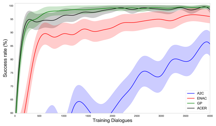
Figure 3: Success rate of ACER compared to other RL methods. Shaded areas represent a 95% confidence interval.

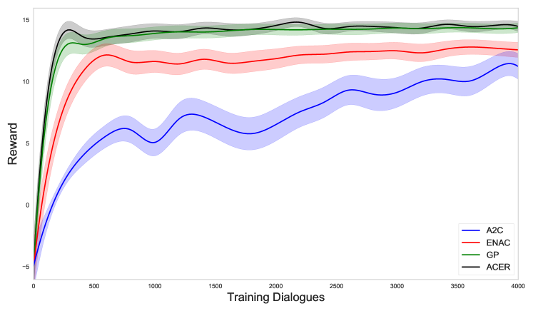
Figure 4: Rewards of ACER compared to other RL methods. Shaded areas represent a 95% confidence interval.

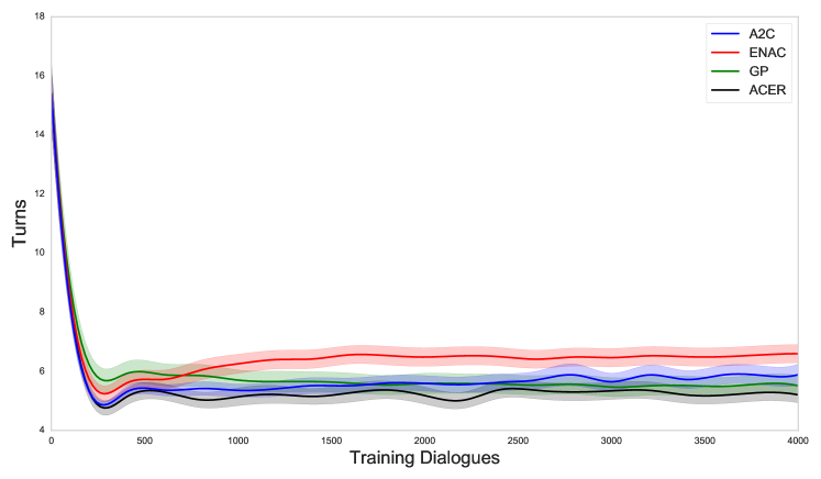
Figure 5: Number of turns for ACER compared to other RL methods. Shaded areas represent a 95% confidence interval.

VII-C Performance of ACER

In the initial environment, the simulated semantic error rate is 0% both for training and testing. The learning rate $\alpha=0.001$. Instead of a simple gradient descent on the loss function, we use the Adam Optimiser, which associates momentum to the gradient [40]. To discourage the algorithm from learning a trivial policy, we subtract 1% of the policy entropy from the loss function. The ACER-specific hyperparameters are: $c=5,\delta=1,\beta=0.99,n=1$. The results are given in Figure 3 and Figure 4 where the shaded are represents a $95\%$ confidence interval.

We observe that ACER is comparable to GP in terms of speed of convergence, sample efficiency, success rate, rewards and turns. While the success rate of ACER remains one or two percentage points below that of GP, ACER requires fewer dialogue turns and ultimately obtains somewhat higher rewards than GP. This suggests that the slightly worse success rate of ACER presents a shortcoming of the reward function rather than the algorithm, as the algorithm only optimises the reward function. We also observe that ACER far exceeds the performance of other NN-based methods in terms of all of speed of convergence, sample efficiency, success rate and rewards.

VII-D Effect of execution mask

We run our experiments with and without the execution mask and compare success rates (Figure 3 and Figure 6).

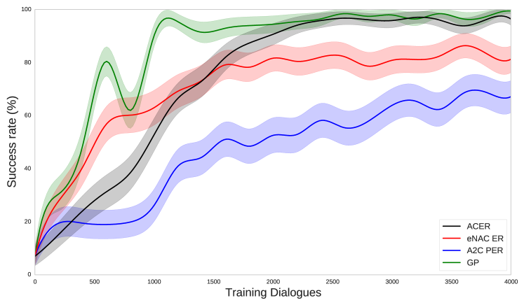
Figure 6: Success rate of ACER compared to other RL methods, without the execution mask. Shaded areas represent a 95% confidence interval.

In general, as expected, algorithms converge slower without the execution mask, while the final performance of GP and ACER remain somewhat below their performances with the mask. This is also expected as a mapping learned by RL is rarely as precise as a hard-coded solution to a problem (execution mask). GP shows faster initial convergence than ACER, as the latter shows a more steady progress without unexpected dips in performance. They remain comparable in every other regard.

VII-E Hyperparameter tuning

ACER has several additional hyperparameters compared to more traditional algorithms. We investigate the effect of hyperparameters $c,\delta,\beta,\mbox{ and }n$ on the algorithm’s performance. To better illustrate the differences, we run the tests in a more challenging setting, without the execution mask. For every analysed parameter, we kept the rest of the hyperparameters set to values providing the best results from section $C$.

Importance Weight threshold $c$

This value is the upper bound of IS weight; weights higher than $c$ are truncated. Setting this value too high diminishes the effect of weight truncation, while a value too low will rely more on the less accurate bias correction term. From Figure 7, we see that $c=5$ delivers the highest convergence rate and a good final performance. We also see that for the wide range of values from $c=1$ to $c=20$, there is no big difference in final performance, suggesting that the algorithm is relatively stable in face of varying this hyperparameter.

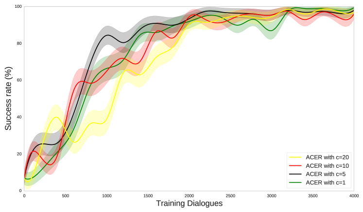
Figure 7: Success rate of ACER with varying hyperparameter $c$. Shaded areas represent a 95% confidence interval.

KL divergence constraint $\delta$

This value constrains the KL divergence between an updated policy and the running average policy. Setting it too high allows radical jumps, setting it too low slows the convergence down (Figure 8). We can see that a setting of $\delta=10$ or $\delta=50$ results in erratic changes in the performance of ACER, while $\delta=0.5$ and $\delta=1$ are sensible choices.

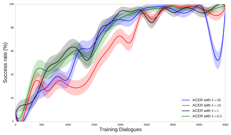
Figure 8: Success rate of ACER with varying hyperparameter $\delta$. Shaded areas represent a 95% confidence interval.

Average policy update weight $\beta$

In Figure 9, we can see that for $\beta\leq 0.9$, the average policy forgets the history too quickly, allowing the policy to gain momentum in any direction and thus preventing it from converging to a good performance. For $\beta=0.95$, the policy converges quickly, while $\beta=0.99$ results in a somewhat conservative algorithm, where the KL divergence constraint keeps the policy near a slowly changing average. $\beta=0.99$ still converges to a good result, but does so somewhat slower than in case of $\beta=0.95$.

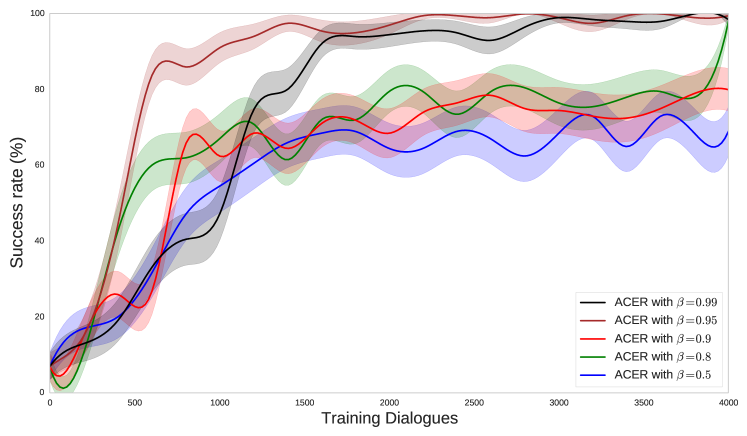
Figure 9: Success rate of ACER with varying hyperparameter $\beta$. Shaded areas represent a 95% confidence interval.

Training iterations $n$

Setting the number of training steps per episode $n$ higher allows the algorithm to learn more from the gathered experience. However, if $n$ is too high, the training might diverge due to the policy moving too much (Figure 10). For $n=1$, convergence is quick and performance is good, while for $n=10$, performance stays poor throughout. For $n=30$ and $n=50$, the algorithm diverges completely.

Figure 10: Success rate of ACER with varying hyperparameter $n$. Shaded areas represent a 95% confidence interval.

VII-F Master action space

ACER compares favourably to other NN-based algorithms, but performs about equally if not slightly worse than GP in our experiments. The experiments were run on the summary action space, which only has $15$ actions. In a more difficult scenario, we may have orders of magnitude more actions. In such scenarios, the computational cost of GPs can be prohibitive as it needs to invert the Gram matrix [21]. If ACER still performs well under the same scenario, it might may be the overall best method to apply to larger action spaces. This is because ACER does not have the prohibitive computational cost of GP, and is expected to train much more quickly.

To test our hypotheses, we deploy ACER on the master action space according to Section V-B1, and on the summary space (Figure 11). Both experiments were run with the execution mask. Convergence is slower on the master action space. This is expected due to having to choose between vastly higher number of actions on the master action space ($1035$ as opposed to $15$). However, ACER is still surprisingly effective on the master action space, converging to about the same performance as on the summary space. We note that this is without any modification to the training algorithm, only the underlying NN is changed. ACER achieves the best results in terms of speed of convergence and final performance on master action space out of NN-based SDS policy optimiser algorithms.

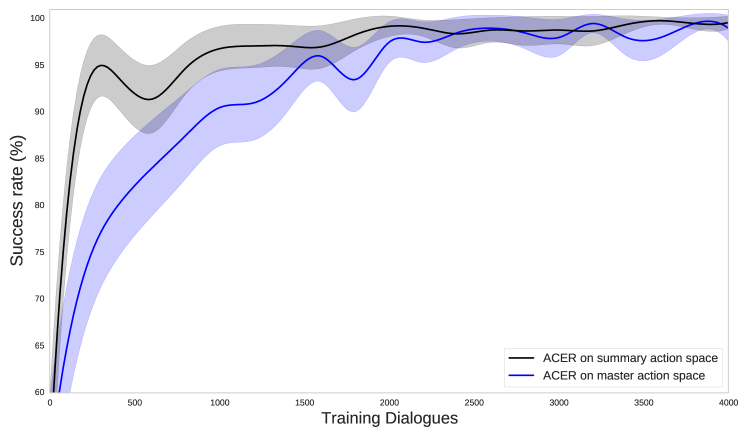
Figure 11: Success of ACER on summary action space compared to ACER on master action space with execution mask. Shaded areas represent a 95% confidence interval.

To investigate further whether ACER is the best choice of algorithm on the master action space, we modify GP to run on master action space according to Section V-B2. We compare ACER and GP both on summary and master action spaces, without the execution mask in Figure 12. Both GP and ACER show slower speed of convergence on master action space. This is expected, as the random initialisation of a policy on master action space will be much less sensible than an initialisation on the summary space, the latter taking advantage of the hard-coded summary to master action mapping method. However, it is surprising to see that all experiments converged to roughly the same performance of about 97% success rate, except for GP on summary, which has a final success rate of 98%-99%. This suggests that both ACER and GP can handle large action spaces quite efficiently. To our knowledge, this is the first time learning on the master action space from scratch was successfully attempted.

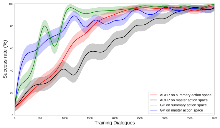
Figure 12: Success of ACER and GP on summary and master action spaces, without execution mask. Shaded areas represent a 95% confidence interval.

GP is more sample efficient than ACER on the challenging master action space without execution mask. However, it requires vastly more computational resources to run: this experiment took $6.45$ hours to run with ACER, and $8.63$ days with GP. Arguably, the extra computational cost overshadows the disadvantage of ACER, that it has to be run for more iterations to converge.

VII-G Noise robustness

So far, our experiment settings were quite idealised, training and testing policies under a perfect simulator with no semantic errors. However, in real life the automatic speech recognition (ASR) component is very likely to make errors as well as the spoken language understanding (SLU) component. Therefore, in reality, the pipeline surrounding the policy optimiser deals with substantial uncertainty, which tends to introduce errors [41]. We ultimately want to measure how well a policy optimiser can learn the optimal strategy in face of noisy semantic-level input. In our experiments, we control this by the semantic error rate, the rate at which a random noisy input is introduced to the optimiser to simulate an error scenario. In other words, a 15% semantic error rate means that with 0.15 probability a semantic concept (slot, value or dialogue act type) presented to the dialogue manager is incorrect. We focus on two desirable properties of a policy. First, ideally, the policy would learn not to trust the input as much, and ask questions until it is sure about the user goal, just like a real human would if the telephone line is noisy. Second, an ideal policy would not only adjust to the error rate of the training conditions, but would dynamically adjust to the conditions of the dialogue it is in. If the policy adjusts too much to the training conditions, it is said to overfit. This could severely limit the policy’s deployability.

We test key algorithms for these two desirable properties. eNAC, the best known NN-based policy optimiser [5] to this date, is compared to ACER and GP. ACER and GP are also compared to their respective variants in master action space. We run the test as follows: first, we train the algorithms under $15\%$ semantic error rate until convergence, with the execution mask. Then we take the fully trained policy and test it under a range of semantic error rates, ranging from $0\%$ to $50\%$ to measure the policies’ generalisation properties. This is something that is never the case in games so this aspect of learning is rarely examined but it is of utmost importance for spoken dialogue systems. We present results in Figure 13 and Figure 14 with a 95% confidence interval.

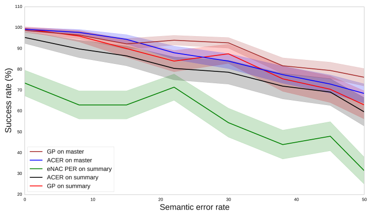
Figure 13: Success rate of key algorithms when training them on 15% and testing them on varying error rates. Shaded areas represent a 95% confidence interval.

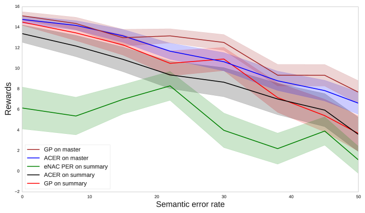
Figure 14: Rewards of key algorithms when training them on 15% and testing them on varying error rates. Shaded areas represent a 95% confidence interval.

Success rate and reward follow the same trends. As expected, we see a general downwards trend for each algorithm as the semantic error rate increases. There is however no apparent spike in performance at the 15% semantic error rate of the training process, indicating that none of the algorithms overfit to this setting. We can see that the performance of eNAC is far behind all the other algorithms. ACER and GP are closer in performance, but GP on summary space consistently beats ACER on summary space.

It might be surprising that both ACER and GP perform better when trained on the master action space as opposed to the summary space, given that they performed worse in previous experiments. However, those experiments had no semantic errors, and a hand-crafted rigid mapping from summary actions to master actions, that relied on the belief state to find the best payload for an inform action. Under a higher semantic error rate, the belief state will be noisy and this mapping may not perform optimally. This highlights the benefits of expanding the scope of artificial intelligence in SDS: AI can be more versatile than hand-coded mappings, especially when the mapping performs decision making under uncertainty.

VII-H Human evaluation

In the previous sections, the training and testing is performed on the same simulated user. To test the generalisation capabilities of the proposed methods, we evaluate the trained dialogue policies in interaction with human users in a similar set-up as in [42]. To recruit the users, we use the Amazon Mechanical Turk (AMT) service where volunteers can call our dialogue system and rate it. Around $900$ dialogues were gathered. Three policies (GP and ACER on summary action space and ACER on master action space) were trained with $15\%$ semantic error rate to accommodate for ASR errors using set-up from previous sections. Then, learnt policies were incorporated into SDS pipeline with a commercial ASR system.

The MTurk users were asked to find restaurants that have particular features as defined by the given task. Subjects were randomly allocated to one of the three analysed systems. After each dialogue the users were asked whether they judged the dialogue to be successful or not which is then translated to a reward measure. Table I presents averaged results with one standard deviation. All models differ indiscernibly with regards to success rate performing very well. However, ACER trained on master action space achieves considerably higher reward (and in turn smaller number of turns) than models working on summary action space.

TABLE I: Human evaluation

	GP summary	ACER summary	ACER master
Success rate	89.7%	88.7%	89.1%
Reward	11.29 ($\pm$ 7.54)	11.39 ($\pm$ 7.17)	11.83 ($\pm$ 8.05)
No. of turns	6.61 ($\pm$ 3.12)	6.42 ($\pm$ 2.84)	5.98 ($\pm$ 3.22)

VIII Conclusion

The policy optimisation algorithms presented in this paper improves the state-of-the-art in spoken dialogue systems (SDS) in three ways:

• A version of ACER [12] designed for SDS s shows better results than the current state-of-the-art for neural network-based policy optimisers [5].

• This implementation of ACER is also able to train efficiently in the master action space, showing the best performance among neural network-based policy optimisers, as reported by [6] and [5].

• Our implementation of GP with a redesigned kernel function achieves the best performance on master action space, which previously was not possible.

GP suffers from an inherently high computational cost, making the algorithm unsuitable in higher volume action spaces. In such cases, the fact that ACER can be trained well on the master action space indicates that it may be the best currently known method to train policies with large action spaces.

As agents powered by machine learning gain more intelligence, they can be applied to more challenging domains. Using the master action space is a good example of this: a hard-coded mapping between summary and action spaces can be used to simplify the task of the AI agent. However, as we have shown, it is no longer required to train in this action space. There is an algorithm (ACER) that can finally bridge the semantic gap between summary and master action spaces without the help of domain-specific code written explicitly for this mapping. This has three benefits: first, training on master action space outperforms the mapping based on fixed code, when uncertainty (semantic errors) is involved. Second, it allows us to build a more generally applicable system, with less work required to deploy it in differing domains. Third, it allows us to consider domains that have vastly higher action spaces, even if there is no clear way to convert those action spaces into small summary action spaces (such as a general purpose dialogue system).

ACER fits well into other SDS research directions too. Successful policy optimisers need to be sample efficient and be able to be trained quickly, to avoid subjecting human users to poor dialogue performance for long. ACER uses experience replay for sample efficiency, together with many methods aimed at reducing bias and variance of the estimator, to achieve quick training.

We introduce some of the many directions in which this work could be continued. Recently, [5] combined supervised learning (SL) with deep reinforcement learning (DRL) to investigate the performance of an agent bootstrapped with SL and trained further with DRL. The NN s of ACER are compatible with that approach. This may decrease the overall interactions required for convergence, as well as increase sample efficiency.

Both of our settings, training on summary and on master action space, considered static action spaces only. Under this framework, the entire policy would have to be retrained if a new action or payload were to be introduced. This could hurt the maintainability of a real-life dialogue system, as it would be expensive to extend the database schema or the list of actions. Ideally, the training algorithm could adapt to such changes made, being able to retain its pre-existing knowledge of the old actions and this is an important topic to investigate in the future.

Appendix A CamInfo action space

We define the action space in the CamInfo restaurants domain. Most information-seeking domains have a similar overall architecture.

• request + slot where slot is an informable slot such as area, food, or pricerange. This action prompts the user to specify their criteria on a slot, eg. “Which area are you interested in?”

• confirm + slot where slot is an informable slot. This action prompts the user to confirm their criteria on a slot that they may or may not have already mentioned. Due to errors accumulating during the decoding pipeline (speech recognition, semantic decoding, belief tracking), the system has to deal with considerable uncertainty, but it can attempt to increase its certainty in the user’s criteria by using a confirm action, eg. “Did you say you want an expensive restaurant?”

• select + slot where slot is an informable slot. This action prompts a user to select a value for the slot from a specified list of values. This is less open-ended than a request action and more open-ended than a confirm action, eg. “Would you like Indian or Korean food?”.

• inform + method + slots action provides information on a restaurant. The associated method specifies how the restaurant to give information on should be chosen. The standard method is to choose the first result in the ontology that matches the user criteria specified so far. The method can also be byname, in which case the system believes that the user asked about a specific restaurant by referring to its name, and information on that restaurant should be provided. If the method is requested, we inform on the same restaurant we informed on last, if it is alternatives then we pick another restaurant that matches the user’s criteria (if possible).

  There are several properties of a restaurant, with a binary choice for each of them on whether the system wants to inform on it in a dialogue turn or not. The informable slots for restaurants are: area, food type, description, phone number, price-range, address, postcode and signature.

  We note that some of these slots are also requestable, allowing a user to query a restaurant based on those slots. These slots are area, food type and price-range. A restaurant also has a name, which we will always inform on. Thus, the system has a choice between $2^{8}=256$ different ways it can inform on a restaurant. A specific choice is referred to as the payload of an inform action.

• reqmore is a simple action that prompts the user to provide more input.

• bye is used to end the call, normally only as a response to the user’s intention to end the call.

For the CamInfo domain, there are $4\cdot 2^{8}=1024$ inform actions and $3\cdot 3+2=11$ other actions, making up $1035$ actions in total. We call this action space the master action space. In the summary space, the inform actions do not specify which slots to inform on, leaving only $4$ separate inform actions, and $15$ actions in total.

Appendix B Example dialogue

Below is an example dialogue between a user looking for a restaurant with a medium price range, and a system that internally translates between summary and master actions. System responses are written as $\mbox{Sys: }\mbox{summary\_action}\rightarrow\mbox{master\_action}$:

$$Sys: \;\mbox{hello()}\rightarrow\mbox{hello()}$$

$$User:$$  inform(type=restaurant)

$$Sys: \;\mbox{request\_pricerange()}\rightarrow\mbox{request\_pricerange()}$$

$$User:$$  inform(pricerange=moderate)

$$Sys: \;\mbox{inform()}\rightarrow\mbox{inform(food="turkish", }\mbox{name="efes restaurant")}$$

$$User:$$  reqalts()

$$Sys: \;\mbox{inform\_alternatives()}\rightarrow\mbox{inform(food="turkish", }\mbox{name="anatolia")}$$

$$User:$$  request(phone)

$$Sys: \;\mbox{inform\_requested}\rightarrow\mbox{inform(name="anatolia",}\mbox{phone="01223 362372")}$$

$$User:$$  thankyou()

$$Sys:$$  bye()

Gellért Weisz received his B.A. degree from the Computer Science Tripos at the University of Cambridge in 2016. He stayed at Cambridge as an MPhil student reading Machine Learning, Speech and Language Technology. Afterwards, he joined Deepmind as a Research Engineer.

Paweł  Budzianowski received his B.A. and M.A. degrees from the Faculty of Mathematics and Computer Science at Adam Mickiewicz University in Poznań in 2015. Since then he has been at the University of Cambridge first as an MPhil student reading Machine Learning, Speech and Language Technology. Afterwards, he has begun a PhD in the Dialogue Systems Group at the University of Cambridge. His research interests include multi-domain policy management and Bayesian deep learning.

Pei-Hao (Eddy) Su is a PhD candidate under the supervision of Professor Steve Young in Dialogue Systems Group at Cambridge University. His research interests centre on applying deep learning, reinforcement learning and Bayesian approaches to dialogue management and reward estimation, with the aim of building systems that can learn directly from human interaction. He has published around 30 peer-reviewed papers across top speech and NLP conferences and he received the best student paper award at ACL 2016.

Milica Gašić is a Lecturer in Spoken Dialogue Systems at the Cambridge University Engineering Department and a Fellow of Murray Edwards College. She holds a BS in Computer Science and Mathematics from the University of Belgrade (2006), an MPhil in Computer Speech, Text and Internet Technology (2007) and a PhD in Engineering from the University of Cambridge (2011). The topic of her PhD was statistical dialogue modelling and she was awarded an EPSRC PhD plus award for her dissertation. She has published around 50 journal articles and peer reviewed conference papers and received a number of best paper awards. She is an elected committee member of IEEE SLTC and an appointed board member of Sigdial.

References

- [1] N. Roy, J. Pineau, and S. Thrun, “Spoken dialogue management using probabilistic reasoning,” in Proceedings of SigDial, 2000.
- [2] S. J. Young, “Talking to machines (statistically speaking),” 7th International Conference on Spoken Language Processing, 2002.
- [3] S. Young, M. Gašić, B. Thomson, and J. D. Williams, “Pomdp-based statistical spoken dialog systems: A review,” Proceedings of the IEEE, vol. 101, no. 5, pp. 1160–1179, 2013.
- [4] J. D. Williams, K. Asadi, and G. Zweig, “Hybrid code networks: practical and efficient end-to-end dialog control with supervised and reinforcement learning,” Association for Computational Linguistics, pp. 665–677, 2017.
- [5] P.-H. Su, P. Budzianowski, S. Ultes, M. Gasic, and S. Young, “Sample-efficient actor-critic reinforcement learning with supervised data for dialogue management,” Proceedings of SigDial, pp. 147–157, 2017.
- [6] M. Fatemi, L. E. Asri, H. Schulz, J. He, and K. Suleman, “Policy networks with two-stage training for dialogue systems,” Proceedings of SigDial, pp. 101–110, 2016.
- [7] T.-H. Wen, D. Vandyke, N. Mrkšić, M. Gašić, L. M. Rojas-Barahona, P.-H. Su, S. Ultes, and S. Young, “A network-based end-to-end trainable task-oriented dialogue system,” in EACL, 2017.
- [8] T. Zhao and M. Eskenazi, “Towards end-to-end learning for dialog state tracking and management using deep reinforcement learning,” in Proceedings of SigDial, 2016, pp. 1–10.
- [9] B. Dhingra, L. Li, X. Li, J. Gao, Y.-N. Chen, F. Ahmed, and L. Deng, “Towards end-to-end reinforcement learning of dialogue agents for information access,” in Association for Computational Linguistics, 2017, pp. 484–495.
- [10] X. Li, Y.-N. Chen, L. Li, J. Gao, and A. Celikyilmaz, “End-to-end task-completion neural dialogue systems,” in International Joint Conference on Natural Language Processing, 2017, pp. 733–743.
- [11] B. Liu and I. Lane, “Iterative policy learning in end-to-end trainable task-oriented neural dialog models,” IEEE Automatic Speech Recognition and Understanding Workshop, 2017.
- [12] Z. Wang, V. Bapst, N. Heess, V. Mnih, R. Munos, K. Kavukcuoglu, and N. de Freitas, “Sample efficient actor-critic with experience replay,” International Conference on Learning Representations, 2017.
- [13] R. Munos, T. Stepleton, A. Harutyunyan, and M. Bellemare, “Safe and efficient off-policy reinforcement learning,” in Advances in Neural Information Processing Systems, 2016, pp. 1046–1054.
- [14] H. Bunt, “Context and dialogue control,” THINK Quarterly, vol. 3, 1994.
- [15] D. R. Traum, “20 questions on dialogue act taxonomies,” JOURNAL OF SEMANTICS, vol. 17, pp. 7–30, 2000.
- [16] M. Henderson, B. Thomson, and S. J. Young, “Deep neural network approach for the dialog state tracking challenge.” in Proceedings of SigDial, 2013, pp. 467–471.
- [17] L. P. Kaelbling, M. L. Littman, and A. R. Cassandra, “Planning and acting in partially observable stochastic domains,” Artificial intelligence, vol. 101, no. 1, pp. 99–134, 1998.
- [18] R. S. Sutton and A. G. Barto, Reinforcement learning: An introduction. MIT press Cambridge, 1998, vol. 1, no. 1.
- [19] M. Gašić, S. Keizer, F. Mairesse, J. Schatzmann, B. Thomson, K. Yu, and S. Young, “Training and evaluation of the his pomdp dialogue system in noise,” Proceedings of SigDial, pp. 112–119, 2008.
- [20] S. Chandramohan, M. Geist, and O. Pietquin, “Optimizing spoken dialogue management with fitted value iteration,” InterSpeech, pp. 86–89, 2010.
- [21] M. Gasic and S. Young, “Gaussian processes for pomdp-based dialogue manager optimization,” IEEE/ACM Transactions on Audio, Speech, and Language Processing, vol. 22, no. 1, pp. 28–40, 2014.
- [22] V. Mnih, K. Kavukcuoglu, D. Silver, A. A. Rusu, J. Veness, M. G. Bellemare, A. Graves, M. Riedmiller, A. K. Fidjeland, G. Ostrovski et al., “Human-level control through deep reinforcement learning,” Nature, vol. 518, no. 7540, pp. 529–533, 2015.
- [23] J. Schulman, S. Levine, P. Abbeel, M. Jordan, and P. Moritz, “Trust region policy optimization,” in International Conference on Machine Learning, 2015, pp. 1889–1897.
- [24] H. Cuayáhuitl, S. Keizer, and O. Lemon, “Strategic dialogue management via deep reinforcement learning,” NIPS Workshop on Deep Reinforcement Learning, 2015.
- [25] Z. C. Lipton, J. Gao, L. Li, X. Li, F. Ahmed, and L. Deng, “Efficient exploration for dialogue policy learning with bbq networks replay buffer spiking,” NIPS Workshop on Deep Reinforcement Learning, 2016.
- [26] J. D. Williams and G. Zweig, “End-to-end lstm-based dialog control optimized with supervised and reinforcement learning,” arXiv preprint arXiv:1606.01269, 2016.
- [27] K. Asadi and J. D. Williams, “Sample-efficient deep reinforcement learning for dialog control,” arXiv preprint arXiv:1612.06000, 2016.
- [28] L.-J. Lin, “Self-improving reactive agents based on reinforcement learning, planning and teaching,” Machine learning, vol. 8, no. 3-4, pp. 293–321, 1992.
- [29] T. Degris, M. White, and R. S. Sutton, “Off-policy actor-critic,” International Conference on Machine Learning, pp. 179–186, 2012.
- [30] R. S. Sutton, D. A. McAllester, S. P. Singh, Y. Mansour et al., “Policy gradient methods for reinforcement learning with function approximation,” in Advances in Neural Information Processing Systems, vol. 99, 1999, pp. 1057–1063.
- [31] D. Precup, R. S. Sutton, and S. Dasgupta, “Off-policy temporal-difference learning with function approximation,” International Conference on Machine Learning, pp. 417–424, 2001.
- [32] B. Thomson, Statistical methods for spoken dialogue management. Springer Science & Business Media, 2013.
- [33] R. Pascanu and Y. Bengio, “Revisiting natural gradient for deep networks,” International Conference on Learning Representations, 2014.
- [34] J. Peters and S. Schaal, “Natural actor-critic,” Neurocomputing, vol. 71, no. 7, pp. 1180–1190, 2008.
- [35] J. Kober and J. R. Peters, “Policy search for motor primitives in robotics,” in Advances in Neural Information Processing Systems, 2009, pp. 849–856.
- [36] W. Gellért, “Sample efficient deep reinforcement learning for dialogue systems with large action spaces,” MPhil Thesis, University of Cambridge, 2017.
- [37] S. Ultes, L. M. Rojas-Barahona, P.-H. Su, D. Vandyke, D. Kim, I. Casanueva, P. Budzianowski, N. Mrkšić, T.-H. Wen, M. Gašić, and S. J. Young, “Pydial: A multi-domain statistical dialogue system toolkit,” in ACL Demo. Association of Computational Linguistics, 2017.
- [38] J. Peters and S. Schaal, “Policy gradient methods for robotics,” in Intelligent Robots and Systems, 2006 IEEE/RSJ International Conference on. IEEE, 2006, pp. 2219–2225.
- [39] J. Schatzmann, B. Thomson, K. Weilhammer, H. Ye, and S. Young, “Agenda-based user simulation for bootstrapping a pomdp dialogue system,” The Conference of the North American Chapter of the Association for Computational Linguistics, pp. 149–152, 2007.
- [40] D. Kingma and J. Ba, “Adam: A method for stochastic optimization,” International Conference on Learning Representations, 2015.
- [41] X. Li, Y. Chen, L. Li, J. Gao, and A. Çelikyilmaz, “Investigation of language understanding impact for reinforcement learning based dialogue systems,” CoRR, vol. abs/1703.07055, 2017.
- [42] F. Jurčíček, S. Keizer, M. Gašić, F. Mairesse, B. Thomson, K. Yu, and S. Young, “Real user evaluation of spoken dialogue systems using Amazon Mechanical Turk,” in INTERSPEECH, 2011.