Artificial intelligence meets minority game: toward optimal resource allocation

Abstract

Complex resource allocation systems provide the fundamental support for the normal functioning and well being of the modern society. Computationally and mathematically, such systems can be modeled as minority games. A ubiquitous dynamical phenomenon is the spontaneous emergence of herding, where a vast majority of the users concentrate on a small number of resources. From an operational point of view, herding is of grave concern as the few overused resources can be depleted quickly, directing users to the next few resources and causing them to fail, and so on, and eventually leading to a catastrophic collapse of the whole system in short time. To devise strategies to prevent herding from occurring is thus of interest. Previous works focused on control strategies that rely on external interventions, such as pinning control where a fraction of users are forced to choose a certain action. Is it possible to eliminate herding without any external control? The main point of this paper is to provide an affirmative answer through exploiting artificial intelligence (AI). In particular, we demonstrate that, when agents are empowered with reinforced learning (e.g., the popular Q-learning in AI) in that they get familiar with the unknown game environment gradually and attempt to deliver the optimal actions to maximize the payoff, herding can effectively be eliminated. Furthermore, computations reveal the striking phenomenon that, regardless of the initial state, the system evolves persistently and relentlessly toward the optimal state in which all resources are used efficiently. However, the evolution process is not without interruptions: there are large fluctuations that occur but only intermittently in time. The statistical distribution of the time between two successive fluctuating events is found to depend on the parity of the evolution, i.e., whether the number of time steps in between is odd or even. We develop a physical analysis and derive mean-field equations to gain an understanding of these phenomena. As minority game dynamics and the phenomenon of herding are common in social, economic, and political systems, and since AI is becoming increasingly widespread, we expect our AI empowered minority game system to have broad applications.

Keywords: Self-Organized Processes, Resource Allocation, Artificial Intelligence, Minority Game, Reinforcement Learning

1 Introduction

The tremendous development of information technology has made it possible for artificial intelligence (AI) to penetrate into every aspect of the human society. One of the fundamental traits of AI is decision making - individuals, organizations, and governmental agencies tend to rely more and more on AI to make all kinds of decisions based on vast available information in an ever increasingly complex environment. At the present, whether a strong reliance on AI is beneficial or destructive to the mankind is an issue of active debate that attracts a great deal of attention from all the professions. In the vast field of AI related research, a fundamental issue is how AI affects or harnesses the behaviors of complex dynamical systems. In this paper, we address this issue by focusing on complex resource allocation systems that incorporate AI in decision making at the individual agent level, and demonstrate that AI can be quite advantageous for complex systems to reach their optimal states.

Resource allocation systems are ubiquitous and provide fundamental support for the modern economy and society, which are typically complex systems consisting of a large number of interacting elements. Examples include ecosystems of different sizes, various transportation systems (e.g., the Internet, urban traffic systems, rail and flight networks), public service providers (e.g., marts, hospitals, and schools), as well as social and economic organizations (e.g., banks and financial markets). In a resource allocation system, a large number of components/agents compete for limited public resources in order to maximize payoff. The interactions among the agents can lead to extremely complex dynamical behaviors with negative impacts on the whole system, among which irrational herding is of great concern as it can cause certain resources to be overcrowded but leave others unused and has the potential to lead to a catastrophic collapse of the whole system in relatively short time. A general paradigm to investigate the collective dynamics of resource allocation systems is complex adaptive systems theory [1, 2, 3]. At the microscopic level, multi-agent models such as the minority game model [4] and interaction models based upon the traditional game theory [5, 6, 7] have been proposed to account for the interactions among the individual agents.

Minority game is a paradigmatic model for resource allocation in population, which was introduced in 1997 [4] for quantitatively studying the classic El Farol bar-attendance problem first conceived by Arthur in 1994 [8]. In the past two decades, minority game and its variants were extensively studied [9, 10, 11, 12, 13, 14, 15, 16, 17, 18, 19, 20, 21, 22, 23, 24, 25, 26, 27, 28, 29, 30, 31, 32, 33, 34, 35], where a central goal was to uncover the dynamical mechanisms responsible for the emergence of various collective behaviors. In the original minority game model, an individual’s scheme for state updating (or decision making) is essentially a trial-and-error learning process based on the global historical winning information [4]. In other models, learning mechanisms based local information from neighbors were proposed [11, 16, 17, 12, 25, 28, 31, 32, 33, 34, 35]. The issue of controlling and optimizing complex resource allocation systems was also investigated [32], e.g., utilizing pinning control to harness the herding behavior, where it was demonstrated that a small number of control points in the network can suppress or even eliminate herding. A theoretical framework for analyzing and predicting the efficiency of pinning control was developed [32], revealing that the connecting topology among the agents can play a significant role in the control outcome. Typically, control requires external interventions. A question is whether herding can be suppressed or even eliminated without any external control.

In this paper, we address the question of how AI can be exploited to harness undesired dynamical behaviors to greatly benefit the operation of the underlying complex system. More generally, we aim to study how AI affects the collective dynamics in complex systems. For this purpose, we introduce a minority game model incorporating AI at the individual agent level, where the agents participating in the game are “intelligent” in the sense that they are capable of reinforced learning [36], a powerful learning algorithm in AI. Empowered with reinforced learning, an agent is capable of executing an efficient learning path toward a pre-defined goal through a trial-and-error process in an unfamiliar game environment. Our model is constructed based on the interplay of a learning agent and the environment in terms of the states, actions, rewards, and decision making. In reinforced learning, the concepts of value and value functions are key to intelligent exploration, and there have been a number of reinforced learning algorithms, such as dynamic programming [36, 37], Monte Carlo method [36, 37], temporal differences [36, 38], Q-Learning [36, 39, 40], Sarsa [36], and Dyna [36], etc. To be illustrative, we focus on Q-learning, which was demonstrated previously to perform well for a small number of individuals in their interaction with an unknown environment [41, 42, 43, 41, 44]. However, here we consider minority game systems with a large number of “intelligent” players, where Q-learning is adopted for state updating in a stochastic dynamical environment. The question is whether the multi-agent AI minority game system can self-organize itself to generate optimal collective behaviors. Our main result is an affirmative answer to this question. Particularly, we find that the population of AI-empowered agents can approach the optimal state of resource utilization through self-organization regardless of the initial state, effectively eliminating herding. However, the process of evolution toward the optimal state is typically disturbed by intermittent, large fluctuations (oscillations) that can be regarded as failure events. There can be two distinct types of statistical distributions of the “laminar” time intervals in which no failure occurs, depending on their parity, i.e., whether the number of time steps between two consecutive failures is odd or even. We develop a physical analysis and use the mean-field approximation to understand these phenomena. Our results indicate that Q-learning is generally powerful in optimally allocating resources to agents in a complex interacting environment.

2 Model

Our minority game model with agents empowered by Q-learning can be described, as follows. The system has $N$ agents competing for two resources denoted by $r=+1$ and $-1$, and each agent chooses one resource during each round of the game. The resources have a finite capacity $C_{r}$, i.e., the maximum number of agents that each resource can accommodate. For simplicity, we set $C_{r}=N/2$. Let $A(t)$ denote the number of agents selecting the resource $r=+1$ at time step $t$. For $A(t)\leq C_{r}$, agents choosing the resource $+1$ belong to the minority group, and win the game in this round. Conversely, for $A(t)>C_{r}$, the resource $+1$ is overcrowded, so the corresponding agents fail in this round.

The Q-learning adaptation mechanism [40] is incorporated into the model by assuming that the states of the agents are parameterized through $Q$ functions that characterize the relative utility of a particular action. The $Q$ functions are updated during the course of the agents’ interaction with the environment. Actions that lead to a higher reward are reinforced. To be concrete, in our model, agents are assumed to have four available actions, and we let $Q(s,a)$ be the $Q$ value of the corresponding action at time $t$, where $s$ and $a$ denote the current state of agent and the action that the agent may take, respectively. A $Q$ function can then be expressed in the following form:

$$\mathbf{Q}={\left[\begin{array}[]{ccc}Q(+1,+1)&Q(+1,-1)\\ Q(-1,+1)&Q(-1,-1)\end{array}\right]}.$$

For an agent in state $s$, after selecting a given action $a$, the corresponding $Q$ value is updated according to the following rule:

$$Q_{t}(s,a)=Q_{t-1}(s,a)+\alpha[R+\gamma Q_{t-1}^{\mathrm{max}}(s^{\prime},a^{\prime})-Q_{t-1}(s,a)],$$ (1)

where $\alpha\in(0,1]$ is the learning rate and $R$ is the reward from the corresponding action. The parameter $\gamma\in[0,1)$ is the discount factor that determines the importance of future reward. Agents with $\gamma=0$ are “short sighted” in that they consider only the current reward, while those with larger values of $\gamma$ care about reward in the long run. The quantity $Q_{t-1}^{\mathrm{max}}(s^{\prime},a^{\prime})$ is the maximum element in the row of the $s^{\prime}$ state, which is the outcome of the action $a$ based on $s$. Equation (1) indicates that the matrix $\mathbf{Q}$ contains information about the accumulative experience from history, where the reward $R$ (for action $a$ from state $s$) and the expected best value $Q_{t-1}^{\mathrm{max}}(s^{\prime},a^{\prime})$ based on $s^{\prime}$ both contribute to the updated value $Q_{t}(s,a)$ with the weight $\alpha$, and the previous value $Q_{t-1}(s,a)$ is also accumulated into $Q_{t}(s,a)$ with the weight $1-\alpha$.

While agents select the action mostly through reinforced learning, certain randomness can be expected in decision making. We thus assume that a random action occurs with a small probability $\epsilon$, and agents select the action with a large value of $Q(s,a)$ with probability $1-\epsilon$. For a given setting of parameters $\alpha$ and $\gamma$, the Q-learning algorithm is carried out, as follows. Firstly, we initialize the matrix $\mathbf{Q}$ to zero to mimic the situation where the agents are unaware of the game environment, and initialize the state $s$ of each agent randomly to $+1$ or $-1$. Next, for each round of the game, each agent chooses an action $a$ with a larger value of $Q_{t}(s,a)$ in the row of its current state $s$ with probability $1-\epsilon$, or chooses an action $a$ randomly with probability $\epsilon$. The $Q(s,a)$ value of the selected action is then updated according to Eq. (1). The action that leads to the state $s^{\prime}$ identical to the current winning (minority) state has $R=1$, and the action leading to the failed (majority) state has $R=0$. Finally, we take the selected action $a$ to update the state from $s$ to $s^{\prime}$.

Distinct from the standard supervised learning [45], agents adopting reinforced learning aim to understand the environment and maximize their rewards gradually through a trial-and-error process. The coupling or interaction among the agents is established through competing for limited resources. Our AI based minority game model also differs from the previously studied game systems [32] in that our model takes into account agents’ complicated memory and decision making process. For our system, a key question is whether the resulting collective behaviors from reinforced learning may lead to high efficiency or optimal resource allocation in the sense that the number of agents that a resource accommodates is close to its capacity.

3 Self-organization and competition

In the traditional minority game, the dynamical rules stipulate that competition and learning among agents can lead to the detrimental herding behavior, to which game systems composed of less diversified agents are particularly susceptible [33, 32, 34, 35]. In our AI minority game system of agents empowered with reinforced learning, herding is dramatically suppressed. To give a concrete example, we set the parameters for Q learning as: learning rate $\alpha=0.9$, discount factor $\gamma=0.9$, and exploration rate $\epsilon=0.02$. Figure 1(a) shows the temporal evolution of the number $A(t)$ of agents choosing resource $+1$. The main features of the time series are the continuous oscillations of $A(t)$ about the capacity $C_{r}$ of resources, convergence of the oscillation amplitude, and bursts of $A(t)$ that occur intermittently. As the oscillations converge to the optimal state, the two resources $r=+1$ and $r=-1$ play as the minority resource alternatively. The remarkable feature is that the agent population tends to self-organize into a non-equilibrium state with certain temporal pattern in order to reach the highly efficient, optimal state, but the process is interrupted by large bursts (failures or fluctuations).

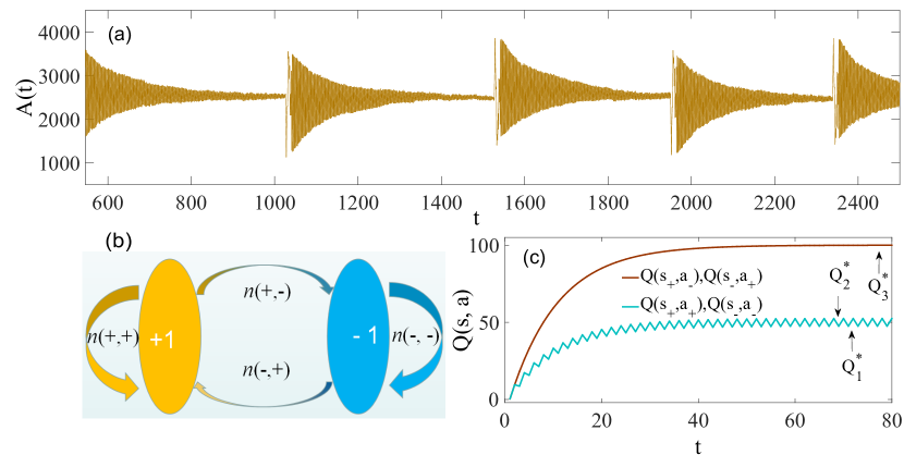
Figure 1: Typical temporal evolutionary behavior of the proposed AI minority game system with reinforced learning empowered agents. (a) Time series of the attendance $A(t)$ of resource $+1$. Interactions among the agents make the system self-organize into a special temporal pattern with two main features: the convergence of regular oscillations towards the optimal value $C_{r}=N/2$, and intermittent bursts of failures in utilizing resources. (b) A schematic sketch of the state transitions of agents during the dynamical process. There are self-satisfied agents in a fixed state and speculative agents that continuously switch state between $+1$ and $-1$. (c) Time series of $Q(s,a)$ as the numerical solutions of Eqs. (2-4). The parameters are: learning rate $\alpha=0.9$, discount factor $\gamma=0.9$, exploration rate $\epsilon=0.02$, and system size $N=5001$.

3.1 Convergence of oscillations

Emergence of two types of agents.

From numerical simulations of the AI minority game system, we find that, as the system self-organizes itself into patterns of regular oscillations, agents with two types of behaviors emerge. The first type is those agents who are “self-satisfied” in the sense that they remain in either the $s=+1$ state or the $s=-1$ state. Those agents win and lose the game alternatively as the system develops regular oscillations. The population sizes of the self-satisfied agents are denoted as $n(+1,+1)$ and $n(-1,-1)$, respectively. The second type of agents are the “speculative” agents, or speculators, who switch state at each time step between $s=+1$ and $s=-1$. These agents always win the game when the system exhibits regular oscillations. We denote the population sizes of the speculative agents as $n(+,-)$ and $n(-,+)$, which correspond to the two possibilities of switching: from $s=+1$ to $s=-1$ and vice versa, respectively.

Figure 1(b) shows the state transition paths induced by the self-satisfied agents and the speculative agents. The oscillations of $A(t)$ associated with the convergent process can be attributed to the state transition of the speculative agents between the states $+1$ and $-1$. This agrees with the intuition that, e.g., the investing behavior of speculators in a financial market is always associated with high risks and large oscillations. Due to the decrease in the population of the speculative agents, the oscillation amplitude in any time interval between two successive failure events tends to decay with time.

Stable state of Q table.

The oscillations of $A(t)$ mean that $r=+1$ and $-1$ act as the minority resource alternatively. For the self-satisfied agents, according to the Q-learning algorithm, the update of the element $Q(s_{+},a_{+})$ can be expressed as,

$$\left\{\begin{array}[]{l}Q_{t+1}(s_{+},a_{+})=Q_{t}(s_{+},a_{+})+\alpha[R+\gamma Q_{t}(s_{+},a_{+})-Q_{t}(s_{+},a_{+})]\\ Q_{t+2}(s_{+},a_{+})=Q_{t+1}(s_{+},a_{+})+\alpha[\gamma Q_{t+1}(s_{+},a_{+})-Q_{t+1}(s_{+},a_{+})]\\ \end{array},\right.$$ (2)

where $Q_{t}^{\mathrm{max}}(s^{\prime},a^{\prime})=Q_{t}(s_{+},a_{+})$ due to the inequality $Q(s_{+},a_{+})>Q(s_{+},a_{-})$. The update of the element $Q(s_{-},a_{-})$ is described by

$$\left\{\begin{array}[]{l}Q_{t+1}(s_{-},a_{-})=Q_{t}(s_{-},a_{-})+\alpha[R+\gamma Q_{t}(s_{-},a_{-})-Q_{t}(s_{-},a_{-})]\\ Q_{t+2}(s_{-},a_{-})=Q_{t+1}(s_{-},a_{-})+\alpha[\gamma Q_{t+1}(s_{-},a_{-})-Q_{t+1}(s_{-},a_{-})]\\ \end{array},\right.$$ (3)

where $Q_{t}^{\mathrm{max}}(s^{\prime},a^{\prime})=Q_{t}(s_{-},a_{-})$ as a result of the inequality $Q(s_{-},a_{-})>Q(s_{-},a_{+})$.

For the speculative agents, the updating equations of elements $Q(s_{+},a_{-})$ and $Q(s_{-},a_{+})$ are

$$\left\{\begin{array}[]{l}Q_{t+1}(s_{+},a_{-})=Q_{t}(s_{+},a_{-})+\alpha[R+\gamma Q_{t}(s_{-},a_{+})-Q_{t}(s_{+},a_{-})]\\ Q_{t+2}(s_{-},a_{+})=Q_{t+1}(s_{-},a_{+})+\alpha[R+\gamma Q_{t+1}(s_{+},a_{-})-Q_{t+1}(s_{-},a_{+})],\\ \end{array}\right.$$ (4)

where $Q_{t}^{\mathrm{max}}(s^{\prime},a^{\prime})=Q_{t}(s_{-},a_{+})$ or $Q_{t}(s_{+},a_{-})$, due to the inequalities $Q(s_{+},a_{+})<Q(s_{+},a_{-})$, and $Q(s_{-},a_{-})<Q(s_{-},a_{+})$.

Figure 1(c) shows numerically obtained time series of the elements of the matrix $\mathbf{Q}$ from Eqs. (2-4). For the self-satisfied agents, the values of $Q(s_{+},a_{+})$ and $Q(s_{-},a_{-})$ increase initially, followed by an oscillating solution between the two values $Q_{1}^{*}$ and $Q_{2}^{*}$, where

$$Q_{1}^{*} = \frac{[1+\alpha(\gamma-1)]\alpha R}{1-[1+\alpha(\gamma-1)]^{2}}$$

$$\mbox{and}\ \ Q_{2}^{*} = \frac{\alpha R}{1-[1+\alpha(\gamma-1)]^{2}}$$

are obtained from Eqs. (2) and (3). For the speculative agents, both $Q(s_{+},a_{-})$ and $Q(s_{-},a_{+})$ reach a single stable solution $Q_{3}^{*}=R/(1-\gamma)$, which can be obtained by solving Eq. (4). The three relevant values have the relationship $Q_{1}^{*}<Q_{2}^{*}<Q_{3}^{*}$.

The emergence of the two types of agents can be understood from the following heuristic analysis. In the dynamical process, a speculative agent emerges when the element associated with an agent satisfies the inequalities $Q(s_{+},a_{-})>Q(s_{+},a_{+})$ and $Q(s_{-},a_{+})>Q(s_{-},a_{-})$ simultaneously. Initially, the agents attend both resources $+1$ and $-1$, with one group winning but the other losing. Only the group that always wins the game can reinforce themselves through further increment in $Q(s_{+},a_{-})$ and $Q(s_{-},a_{+})$. The stable group of speculative agents leads to regular oscillations of $A(t)$, because they switch states together between $+1$ and $-1$. An agent becomes self-satisfied when it is in the $+1$ state and the inequality $Q(s_{+},a_{+})>Q(s_{+},a_{-})$ holds, or in the $-1$ state and $Q(s_{-},a_{-})>Q(s_{-},a_{+})$ holds. The self-satisfied state can be strengthened following the evolution governed by Eqs. (2) and (3), with $Q(s_{+},a_{+})$ or $Q(s_{-},a_{-})$ reaching the oscillating state between $Q_{1}^{*}$ and $Q_{2}^{*}$, as shown in Fig. 1(c). We see that the condition for an agent to become speculative is more strict than to be self-satisfied. Moreover, a speculative agent has certain probability to become self-satisfied, as determined by the value of the exploration rate $\epsilon$. As a result, the population of the speculative agents tends to shrink, leading to a decrease in the oscillation amplitude $|n(+,-)-n(-,+)|$ and convergence of $A(t)$ closer to the optimal state $N/2$.

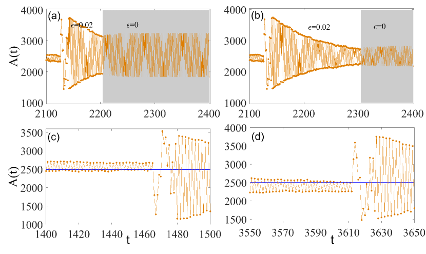
Figure 2: Convergence of regular oscillations and bursts of failure. (a,b) Convergence of the regular oscillation pattern depends on the exploration behavior of the agents as characterized by the rate $\epsilon$. For $\epsilon=0$ (gray region), the oscillation amplitude does not converge. (c,d) Detailed processes for the bursts of failure. If the regular oscillations do not cross the line $C_{r}=N/2$ but behave either as (c) $A(t)>C_{r}$ and $A(t+1)>C_{r}$ or as (d) $A(t)<C_{r}$ and $A(t+1)<C_{r}$, the regular oscillations stop and a systematic failure burst emerges. The blue line specifies $A(t)=C_{r}$. The parameters are the same as in Fig. 1.

For the special case of $\epsilon=0$ [the gray regions in Figs. 2(a) and 2(b)], agents take action entirely based on historical experience $\mathbf{Q}$. In this case, the numbers of the self-satisfied and speculative agents become constant, and $A(t)$ no longer converges to that associated with the optimal state. It is thus apparent that exploration plays a crucial role in the convergence of the system dynamics toward the state in which the resources are optimally utilized.

3.2 Intermittent failures in the AI minority game system

The intermittent bursts of failure events in the whole system take place during the convergent process to the optimal state. An understanding of the mechanism of the failures can provide insights into the articulation of strategies to make the system more robust and resilient.

The criterion to determine if an agent selecting $+1$ wins the minority game is $A(t)<C_{r}=N/2$. If the event $A(t)<C_{r}$ [or $A(t)>C_{r}$] occurs twice in row, the oscillation pattern will be broken. Since the agents are empowered with reinforced learning, two consecutive winnings of either resource $-1$ or resource $+1$ represent an unexpected event, and this would lead to cumulative errors in the $Q$ table, triggering a burst of error in decision making and, consequently, leading to failures in utilizing the resources. To see this in a more concrete way, we note that a self-satisfied agent wins and fails alternatively following a regular oscillation pattern. If the agent fails twice in row, its confidence in preserving the current state is reduced. As a result, the event $Q(s_{+},a_{+})<Q(s_{+},a_{-})$ or $Q(s_{-},a_{-})<Q(s_{-},a_{+})$ would occur with a high probability, leading to a decrease in the populations $n(+,+)$ and $n(-,-)$ of the self-satisfied agents. The populations of the speculative agents, $n(+,-)$ and $n(-,+)$, are increased accordingly. These events collectively generate a bursting disturbance to the regular oscillation pattern of $A(t)$, terminating the system’s convergence toward the optimal state, as shown in Figs. 2(a) and 2(b).

In general, the stability of the regular oscillations depends on two factors: the equilibrium position determined by the self-satisfied agents, and the random fluctuations introduced by agents’ exploration behavior. For the first factor, the equilibrium position is given by $A_{0}=n(+,+)+[n(-,+)-n(+,-)]/2$, which deviates from $C_{r}$ due to the asymmetric distribution of the self-satisfied agents in the two distinct resources. Figures 2(a) and 2(b) show two examples with the equilibrium position $A_{0}$ larger or smaller than $C_{r}$ (the blue solid line), respectively. We see that the converging process is terminated when either the upper or the lower envelope reaches $C_{r}$, i.e., when two consecutive steps of $A(t)$ stay on the same side of $C_{r}$ in replacement of an oscillation about $C_{r}$. In the thermodynamic limit, for an infinitely large system with self-satisfied agents symmetrically distributed between $+1$ and $-1$ (so that the equilibrium position $A_{0}$ is at $C_{r}$), the oscillation would persist indefinitely and $A(t)$ approaches $C_{r}$ asymptotically.

The second factor of random fluctuations in agents’ exploratory behavior is caused by the finite system size, which affects the oscillation stability. As the populations [$n(+,-)$ and $n(-,+)$] of the speculative agents decrease during the converging process, the amplitude of oscillation, $|n(+,-)-n(-,+)|$, becomes comparable to $\sqrt{\epsilon N}$, the level of random fluctuations in the system. The occurrence of two consecutive steps of $A(t)>C_{r}$ (or $A(t)<C_{r}$) as a result of the fluctuations will break the regular oscillation pattern. In the thermodynamical limit, the effects of the random fluctuations are negligible.

3.3 Time intervals between failure bursts

The dynamical evolution of the system can be described as random failure bursts superimposed on regular oscillations with decreasing amplitude. The intermittent failures can be characterized by the statistical distribution of the time interval $T_{0}$ between two successive bursting events. Figure 3(a) shows a representative histogram of $T_{0}$ obtained from a single statistical realization of the system dynamics (the inset’s showing the same data but on a semi-logarithmic scale). A remarkable feature is that the distributions of the odd (red crosses) and even values of $T_{0}$ (blue squares) are characteristically distinct. In particular, the odd values of $T_{0}$ emerge with a smaller probability and the corresponding distribution has a smaller most probable value as compared with that for the even values of $T_{0}$. A possible explanation lies in the existence of two intrinsically distinct processes.

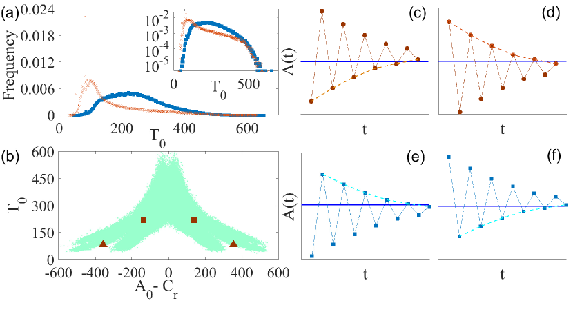
Figure 3: Statistical distributions of the time interval $T_{0}$ between two successive bursts of failure. (a) The distributions obtained from one realization of the system dynamics, where those of the odd $T_{0}$ values (red crosses) and even $T_{0}$ values (blue squares) are remarkably distinct. (b) $T_{0}$ versus the deviation $A_{0}-C_{r}$ of the equilibrium position from the resource capacity. The solid squares (triangles) denote the most probable value of the set of even (odd) $T_{0}$ values. The parameters are $\alpha=0.9$, $\gamma=0.9$, and $N=5001$. (c-f) Schematic illustration of four cases associated with the regular oscillations of $A(t)$, where cases (c,d) lead to odd intervals $T_{0}$ while cases (e,f) lead to the even values of $T_{0}$. The dashed curves represent the envelopes that cross the capacity value $C_{r}$ (solid blue lines), which triggers a failure burst.

Our computation and analysis indicate that the regular oscillation processes can be classified into two categories, as shown in Figs. 3(c-f), leading to insights into the mechanism for the two distinct types of statistical distributions in $T_{0}$. In Fig. 3(c), $A(t)$ starts from a value below $C_{r}=N/2$ and terminates at a value above $C_{r}$, due to the two consecutive values above $C_{r}$ as the lower envelope of $A(t)$ crosses $C_{r}$. Similarly, in Fig. 3(d), $A(t)$ starts from a value above $C_{r}$ and terminates at a value below $C_{r}$, with the upper envelope of $A(t)$ crossing $C_{r}$. In Fig. 3(e), $A(t)$ starts from a value below $C_{r}$ and terminates at a value below $C_{r}$. In Fig. 3(f), $A(t)$ starts from a value above $C_{r}$ and terminates at a value above $C_{r}$. In Figs. 3(c) and 3(d), odd intervals are generated, while in Figs. 3(e) and 3(f), the intervals are even. Between the cases in the same category [e.g., (c,d) or (e,f)], there is little difference in the statistical distribution of $T_{0}$, especially in the long time limit.

We have seen that the equilibrium position $A_{0}$ plays an important role in terminating the regular oscillations, which can be calculated as $A_{0}=\langle A(t)\rangle_{t}$, where $\langle\cdot\rangle_{t}$ denotes the average over time. From Fig. 3(b) where the time interval $T_{0}$ is displayed as a function of the quantity $A_{0}-C_{r}$, we see that the values of $A_{0}$ closer to the capacity $C_{r}$ lead to regular oscillations with larger values of $T_{0}$. The most probable values of the distributions of the even (squares) and odd (stars) $T_{0}$ values are also indicated in Fig. 3(b).

3.4 Mean field theory

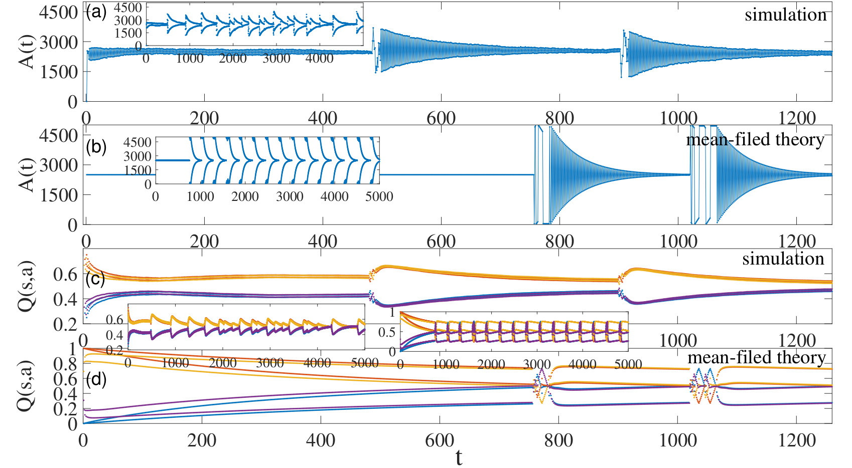
Figure 4: Comparison of dynamical evolution of the system obtained from simulation and mean-field theory. The attendance $A(t)$ obtained from (a) multiagent simulation, and (b) numerical solution of Eqs. (4-9). (c,d) The corresponding results of the elements of $\mathbf{Q}$ from multi-agent simulation and from numerical solution, respectively. The insets in (a-d) show the corresponding time series of $A(t)$ and $\mathbf{Q}$ in a large time regime. The parameters are $\alpha=0.9$, $\gamma=0.9$, $\epsilon=0.02$, and $N=5001$.

We develop a mean-field analysis to capture the main features of the dynamical evolution of the multi-agent AI minority system. We assume that the agents empowered with reinforced learning are identical and share the same matrix $\mathbf{Q}$. The dynamical evolution of $A(t)$ can be described by the following equation:

$$\frac{dA(t)}{dt}=\epsilon\frac{N}{2}+(1-\epsilon)[A(t)\Theta(X_{1})+(N-A(t))\Theta(X_{2})]-A(t),$$ (5)

where the first item $\epsilon N/2$ is the number of agents that act randomly with probability $\epsilon$, half of which select $+1$. The second item indicates the number of agents that act based on the matrix $\mathbf{Q}$ with probability $1-\epsilon$, which include agents that stay in the $+1$ state and those that transition from $-1$ to $+1$. $\Theta(X)$ denotes the step function: $\Theta(X)=0$ for $X<0$, $\Theta(X)=1/2$ for $X=0$, and $\Theta(X)=1$ for $X>0$. The quantities $X_{1}$ and $X_{1}$ are defined as $X_{1}\equiv Q_{t}(s_{+},a_{+})-Q_{t}(s_{+},a_{-})$, and $X_{2}\equiv Q_{t}(s_{-},a_{+})-Q_{t}(s_{-},a_{-})$.

The elements of the matrix $\mathbf{Q}$ are updated according to the following rules:

$$\frac{dQ_{t}(s_{+},a_{+})}{dt} = \alpha[R\Theta(X_{3})+\gamma Q_{t}^{\mathrm{max}}-Q_{t}(s_{+},a_{+})][(1-\epsilon)\Theta(X_{1})+\frac{1}{2}\epsilon],$$ (6)

$$\frac{dQ_{t}(s_{+},a_{-})}{dt} = \alpha[R\Theta(-X_{3})+\gamma Q_{t}^{\mathrm{max}}-Q_{t}(s_{+},a_{-})][(1-\epsilon)\Theta(-X_{1})+\frac{1}{2}\epsilon],$$ (7)

$$\frac{dQ_{t}(s_{-},a_{+})}{dt} = \alpha[R\Theta(X_{3})+\gamma Q_{t}^{\mathrm{max}}-Q_{t}(s_{-},a_{+})][(1-\epsilon)\Theta(X_{2})+\frac{1}{2}\epsilon],$$ (8)

$$\frac{dQ_{t}(s_{-},a_{-})}{dt} = \alpha[R\Theta(-X_{3})+\gamma Q_{t}^{\mathrm{max}}-Q_{t}(s_{-},a_{-})][(1-\epsilon)\Theta(-X_{2})+\frac{1}{2}\epsilon],$$ (9)

where, $X_{3}\equiv N-2A(t)$, the step function $\Theta(X_{3})$ indicates whether or not the agents gain a reward, $Q_{t}^{\mathrm{max}}$ is the expected value after action. Specifically, we have $Q_{t}^{\mathrm{max}}=\max[Q_{t}(s_{+},a_{+}),Q_{t}(s_{+},a_{-})]$ in Eqs. (6) and (8) for the agents who take action to transition to $+1$. Similarly, $Q_{t}^{\mathrm{max}}=\max[Q_{t}(s_{-},a_{+}),Q_{t}(s_{-},a_{-})]$ in Eqs. (7) and (9) is for agents taking action to transition to the state $-1$.

The dynamical evolution of the system can thus be assessed either through simulation, as presented in Figs. 4(a) and 4(c), or through the mean-field equations Eqs. (4-9), as shown in Figs. 4(b) and 4(d). A comparison between These results indicates that the mean-field equations Eqs. (4-9) capture the main features of the collective dynamics of the AI minority system, which are regular oscillations with converging amplitude and intermittent bursts of failure.

4 Discussion

Complex resource allocation systems with a large number of interacting components are ubiquitous in the modern society. Optimal performance of such a system is typically measured by uniform and even utilization of all available resources by the users. Often this is not possible due to the phenomenon of herding that can emerge spontaneously in the evolution of the system, in which most agents utilize only a few resources, leaving the vast majority of the remaining resources little exploited [11, 46, 47, 16, 17, 48, 49, 50, 51, 34, 32, 35]. The heading behavior can propagate through the system, as the few heavily used resources would be depleted quickly, directing most agents to another possibly small set of resources, which would be depleted as well, and so on. A final outcome is the total collapse of the entire system. An important goal in managing a complex resource allocation system is to devise effective strategies to prevent the herding behavior from occurring. We note that similar behaviors occur in economics [52, 53, 54, 55]. Thus any effective methods to achieve optimal performance of resource allocation systems can potentially be generalized to a broader context.

Mathematically, a paradigm to describe and study the dynamics of complex resource allocation is minority games, in which a large number agents are driven to seek the less used resources based on available information to maximize payoff. In the minority game framework, a recent work addressed the problem of controlling heading [33] using the pinning method that had been studied in controlling collective dynamics such as synchronization in complex networks [56, 57, 58, 59, 60, 61, 62, 32], where the dynamics of a small number of nodes are “pinned” to some desired behavior. In developing a pinning control scheme, the fraction of agents chosen to hold a fixed state and the structure of the pinned agents are key issues. For the minority game system, during the time evolution, fluctuations that contain characteristically distinct components can arise: intrinsic and systematic, and this allows one to design a control method based on separated control variables [33]. A finding was that biased pinning control pattern can lead to an optimal pinning fraction that minimizes the system fluctuations, and this holds regardless of the network topologies.

Any control based method aiming to suppress or eliminate herding requires external input. The question we address in this paper is whether it would be possible to design a “smart” type of resource allocation systems that can sense the potential emergence of herding and adjust the game strategy accordingly to achieve the same goal but without any external intervention. Our answer is affirmative. In particular, we introduce AI into the minority game system in which the agents are “intelligent” and empowered with reinforced learning. Exploiting a popular learning algorithm in AI, Q-learning, we find that the collective dynamics can evolve to the optimal state in a self-organized fashion, which is effectively immune from any herding behavior. Due to the complex dynamics, the evolution toward the optimal state is not uninterrupted: there can be intermittent bursts of failures. However, because of the power of self-learning, once a failure event has occurred, the system can self-repair or self-adjust to start a new process of evolution toward the optimal state, free of herding. A finding is that two distinct types of the probability distribution of the intervals of free evolution (the time interval between two successive failure events) arise, depending on the parity of the system state. We provide a physical analysis and derive mean-field equations to understand these behaviors. AI has become increasingly important and has been universally applied to all aspects of the modern society. Our work demonstrates, for the first time, that the marriage of AI with complex systems can generate optimal performance without the need of external control or intervention.

Appendix

Convergence mechanism of $A(t)$

Typically, after a failure burst, $A(t)$ will converge to the value corresponding to the optimal system state. The mechanism of convergence can be understood, as follows. The essential dynamical event responsible for the convergence is the change of agents from being speculative to being self-satisfied within the training time. If the inequalities $Q(s_{+},a_{+})<Q(s_{+},a_{-})$ and $Q(s_{-},a_{-})<Q(s_{-},a_{+})$ hold, the agent is speculative and wins the game all the time as a result of the state transition. Otherwise, for $Q(s_{+},a_{+})>Q(s_{+},a_{-})$ and $Q(s_{-},a_{-})>Q(s_{-},a_{+})$, the agent is self-satisfied and wins and loses the game alternatively.

Consider a speculative agent. Assume that its state is $r=+1$ at the current time step. The agent selects $r=+1$ with the probability $\epsilon/2$ and updates $Q(s_{+},a_{+})$ with reward or selects $r=-1$ with the probability $\epsilon/2+(1-\epsilon)$ and updates $Q(s_{+},a_{-})$ without reward. If the agent selects $r=+1$, the game will be lost, but the value of $Q(s_{+},a_{+})$ can increase. At the next time step, the agent selects $r=-1$ and loses the game, and $Q(s_{+},a_{-})$ will decrease. As a result, the inequality $Q(s_{+},a_{+})>Q(s_{+},a_{-})$ holds with the probability $\epsilon/2$. That is, the probability that a speculative agent changes to a self-satisfied one is approximately $\epsilon/2$.

Now consider a self-satisfied agent in the $r=+1$ state at the current time step. The agent selects $r=+1$ with the probability $\epsilon/2+(1-\epsilon)$ and updates $Q(s_{+},a_{+})$ with two stable solutions ($Q_{1}^{*}$ and $Q_{2}^{*}$), or the agent selects $r=-1$ with the probability $\epsilon/2$. The agent selects $r=-1$ from the two stable solutions $Q_{1}^{*}$ or $Q_{2}^{*}$ with the respective probability $1/2$. If the agent is associated with the smaller stable solution $Q_{2}^{*}$, then $Q(s_{+},a_{-})$ will decrease. As a result, the agent remains to be self-satisfied. If the agent is associated with the larger stable solution $Q_{1}^{*}$, then $Q(s_{+},a_{-})$ will increase due to reward, and the inequality $Q(s_{+},a_{-})>Q(s_{+},a_{+})$ holds with the probability $1/2$. At the same time, if $Q(s_{-},a_{+})>Q(s_{-},a_{-})$, the probability is approximately equal to $1/2$, and the self-satisfied agent successfully becomes a speculative agent. Otherwise, the self-satisfied agent remains to be self-satisfied. That is, the probability that a self-satisfied agent changes to being speculative is approximately $\epsilon/16\ll\epsilon/2$. As a result, $A(t)$ will converge to $C_{r}$ asymptotically.

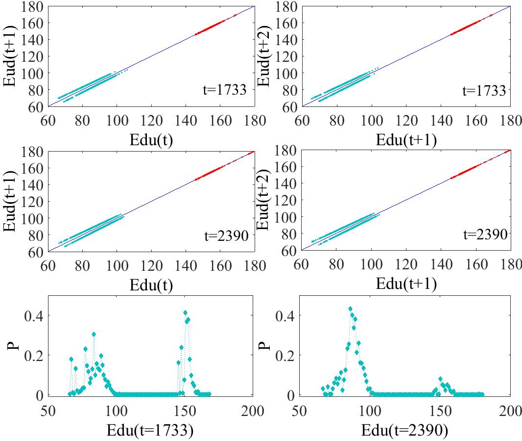
Figure 5: Euclidean distance for all agents empowered with reinforced learning. The distances are indicated by the two red arrow positions in Fig. 1(a). (a-d) Evolution of the Euclidean distance at three adjacent time steps: $t+1$ vs $t$ and $t+2$ vs $t+1$. The blue line is $x=y$. Panels (a,b) correspond to the left arrow, and (c,d) to the right arrow. (e,f) The corresponding distributions of the Euclidean distance.

Two types of agents in the phase space

For the AI minority game system, we can construct the phase space, in which the two types of agents can be distinguished. We define the Euclidean distance for the $\mathbf{Q}$ matrix of each agent as the square root of the sum of all the matrix elements. For the two positions indicated by the red arrows in Fig. 1(a), Figs. 5(a-d) show the relationship of Euclidean distance at three adjacent time steps. We see that the agents can be distinguished and classified into two categories through the Euclidean distance, where the self-satisfied and the speculative agents correspond to the top and bottom sides of the line $x=y$ and on the line $x=y$, respectively. The reason that the speculative agents change their state while the self-satisfied agents remain in their state lies in the property of the elements of the $\mathbf{Q}$ matrix. In particular, after the system reaches a steady state after training, for the speculative agents, the following inequalities hold: $Q(s_{+},a_{+})<Q(s_{+},a_{-})$ and $Q(s_{-},a_{-})<Q(s_{-},a_{+})$, while for the self-satisfied agents, the inequalities are $Q(s_{+},a_{+})>Q(s_{+},a_{-})$ and $Q(s_{-},a_{-})>Q(s_{-},a_{+})$. Since the values of the matrix elements $Q(s_{+},a_{+})$ and $Q(s_{-},a_{-})$ associated with the self-satisfied agents are between $Q_{1}^{*}$ and $Q_{2}^{*}$, the Euclidean distance of these agents rolls over on the line $x=y$ at the adjacent time. However, the elements $Q(s_{+},a_{-})$ and $Q(s_{-},a_{+})$ associated with the speculative agents reach only the stable solution $Q_{3}^{*}$. As a result, the Euclidean distance of these agents remain unchanged. Figures 5(e) and 5(f) show that the Euclidean distances for the agents display a two-peak distribution, corresponding to the two types. The peak height on the left hand side increases with time, while that on the right hand side decreases.

References

- [1] Kauffman S A 1993 The origins of order: Self-organization and selection in evolution (Oxford university press)
- [2] Levin S A 1998 Ecosys. 1 431–436
- [3] Arthur W B, Durlauf S N and Lane D A 1997 The economy as an evolving complex system II vol 28 (Addison-Wesley Reading, MA)
- [4] Challet D and Zhang Y C 1997 arXiv preprint adap-org/9708006
- [5] Nowak M A, Page K M and Sigmund K 2000 Science 289 1773–1775
- [6] Roca C P, Cuesta J A and Sánchez A 2009 Phys. Rev. E 80 046106
- [7] Press W H and Dyson F J 2012 Proc. Nat. Acad. Sci. (UDA) 109 10409–10413
- [8] Arthur W B 1994 Ame. Econ. Rev. 84 406–411
- [9] Challet D and Marsili M 1999 Phys. Rev. E 60 R6271
- [10] Savit R, Manuca R and Riolo R 1999 Phys. Rev. Lett. 82 2203
- [11] Paczuski M, Bassler K E and Corral Á 2000 Phys. Rev. Lett. 84 3185
- [12] Challet D, Martino A D and Marsili M 2008 J. Stat. Mech. Theo. E. L04004
- [13] Moro E 2004 Advances in Condensed Matter and Statistical Physics (Nova Science Publishers) chap The Minority Games: An Introductory Guide
- [14] Challet D, Marsili M and Zhang Y C 2005 Minority Games Oxford Finance (Oxford University Press)
- [15] Yeung C H and Zhang Y C 2009 Minority games Encyclopedia of Complexity and Systems Science ed Meyers R A (Springer New York) pp 5588–5604
- [16] Zhou T, Wang B H, Zhou P L, Yang C X and Liu J 2005 Phys. Rev. E 72 046139
- [17] Eguiluz V M and Zimmermann M G 2000 Phys. Rev. Lett. 85 5659
- [18] Lo T S, Chan K P, Hui P M and Johnson N F 2005 Phys. Rev. E 71 050101
- [19] Johnson N F, Hart M and Hui P M 1999 Physica A 269 1–8
- [20] Hart M, Jefferies P, Johnson N F and Hui P M 2001 Physica A 298 537–544
- [21] Marsili M 2001 Physica A 299 93 – 103 ISSN 0378-4371 application of Physics in Economic Modelling
- [22] Bianconi G, Martino A D, Ferreira F F and Marsili M 2008 Quant. Financ. 8 225–231
- [23] Xie Y B, B H Wang C K H and Zhou T 2005 Eur. Phys. J. B 47 587
- [24] Zhong L X, Zheng D F, Zheng B and Hui P M 2005 Phys. Rev. E 72(2) 026134
- [25] Anghel M, Toroczkai Z, Bassler K E and Korniss G 2004 Phys. Rev. Lett. 92(5) 058701
- [26] Lo T S, Chan H Y, Hui P M and Johnson N F 2004 Phys. Rev. E 70(5) 056102
- [27] Slanina F 2001 Physica A 299 334
- [28] Kalinowski T, Schulz H J and Birese M 2000 Physica A 277 502
- [29] Martino A D, Marsili M and Mulet R 2004 Europhys. Lett. 65 283
- [30] Borghesi C, Marsili M and Miccichè S 2007 Phys. Rev. E 76(2) 026104
- [31] Galstyan A and Lerman K 2002 Phys. Rev. E 66(1) 015103
- [32] Zhang J Q, Huang Z G, Dong J Q, Huang L and Lai Y C 2013 Phys. Rev. E 87(5) 052808
- [33] Zhang J Q, Huang Z G, Wu Z X, Su R Q and Lai Y C 2016 Sci. Rep. 6
- [34] Huang Z G, Zhang J Q, Dong J Q, Huang L and Lai Y C 2012 Sci. Rep. 2 703
- [35] Dong J Q, Huang Z G, Huang L and Lai Y C 2014 Phys. Rev. E 90 062917
- [36] Richard S Sutton A G B 1998 Reinforcement Learning: An Introduction vol 21 (Cambridge MA: The MIT press)
- [37] Bellman R E 1957 Dynamic Programing (Princeton, New Jersey: Princeton University Press)
- [38] Sutton R S 1998 Mach. Learning 3 9–44
- [39] Watkins C J C 1989 PhD Thesis Cambridge University
- [40] Watkins C J C H and Dayan P 1992 Mach. Learning 8 279–292
- [41] Kianercy A and Galstyan A 2012 Phys. Rev. E 85(4) 041145
- [42] Potapov A and Ali M K 2003 Phys. Rev. E 67(2) 026706
- [43] Sato Y and Crutchfield J P 2003 Phys. Rev. E 67(1) 015206
- [44] Kianercy A and Galstyan A 2013 Phys. Rev. E 88(1) 012815
- [45] Das R and Wales D J 2016 Phys. Rev. E 93(6) 063310
- [46] Vázquez A 2000 Phys. Rev. E 62 R4497
- [47] Galstyan A and Lerman K 2002 Phys. Rev. E 66 015103
- [48] Lee S and Kim Y 2004 J. Korean. Phys. Soc. 44 672–676
- [49] Wang J, Yang C X, Zhou P L, Jin Y D, Zhou T and Wang B H 2005 Physica A 354 505–517
- [50] Zhou P L, Yang C X, Zhou T, Xu M, Liu J and Wang B H 2005 New Math. Nat. Comp. 1 275–283
- [51] Huang Z G, Wu Z X, Guan J Y and Wang Y H 2006 Chin. Phys. Lett. 23 3119
- [52] Banerjee A V 1992 Q. J. Econ. 797–817
- [53] Cont R and Bouchaud J P 2000 Macroecon. Dyn. 4 170–196
- [54] Ali S N and Kartik N 2012 Econ. Theor. 51 601–626
- [55] Morone A and Samanidou E 2008 J. Evol. Econ 18 639–646
- [56] Wang X F and Chen G 2002 Physica A 310 521–531
- [57] Li X, Wang X and Chen G 2004 IEEE Trans. Circ. Sys. 51 2074–2087
- [58] Chen T, Liu X and Lu W 2007 IEEE Trans. Circ. Sys. 54 1317–1326
- [59] Xiang L, Liu Z, Chen Z, Chen F and Yuan Z 2007 Physica A 379 298–306
- [60] Tang Y, Wang Z and Fang J a 2009 Chaos 19 013112
- [61] Porfiri M and Fiorilli F 2009 Chaos 19 013122
- [62] Yu W, Chen G and Lü J 2009 Automatica 45 429–435