From acquaintance to best friend forever:
robust and fine-grained inference of social-tie strengths

Abstract.

Social networks often provide only a binary perspective on social ties: two individuals are either connected or not. While sometimes external information can be used to infer the strength of social ties, access to such information may be restricted or impractical.

Sintos and Tsaparas (KDD 2014) first suggested to infer the strength of social ties from the topology of the network alone, by leveraging the Strong Triadic Closure (STC) property. The STC property states that if person $A$ has strong social ties with persons $B$ and $C$, $B$ and $C$ must be connected to each other as well (whether with a weak or strong tie). Sintos and Tsaparas exploited this property to formulate the inference of the strength of social ties as an $\mathbf{NP}$-hard optimization problem, and proposed two approximation algorithms.

We refine and improve this line of work, by developing a sequence of linear relaxations of the problem, which can be solved exactly in polynomial time. Usefully, these relaxations infer more fine-grained levels of tie strength (beyond strong and weak), which also allows to avoid making arbitrary strong/weak strength assignments when the network topology provides inconclusive evidence. One of the relaxations simultaneously infers the presence of a limited number of STC violations. An extensive theoretical analysis leads to two efficient algorithmic approaches. Finally, our experimental results elucidate the strengths of the proposed approach, and sheds new light on the validity of the STC property in practice.

1. Introduction

Online social networks, such as Facebook, provide unique insights into the social fabric of our society. They form an unprecedented resource to study social-science questions, such as how information propagates on a social network, how friendships come and go, how echo chambers work, how conflicts arise, and much more.

Yet, many social networks provide a black-and-white perspective on friendship: they are modeled by unweighted graphs, with an edge connecting two nodes representing that two people are friends. Surely though, some friendships are stronger than others, and clearly, in studying social phenomena understanding the strength of social ties can be critical.

Although in some cases detailed data are available and can be used for inferring the strength of social ties, e.g., communication frequency between users, or explicit declaration of relationship types, such information may not always be available.

The question of whether the strength of social ties can be inferred from the structure of the social network alone, the subject of the current paper, is therefore an important one. Before we discuss our specific contributions, however, let us provide some essential background on prior work on this topic.

Background. An important line of research attempting to address the inference of the strength of social ties is based on the strong triadic closure (STC) property from sociology, introduced by Georg Simmel in 1908 (Simmel, 1908). To understand the STC property, consider an undirected network $G=(V,E)$, with $E\subseteq{V\choose 2}$. Consider additionally a strength function $w:E\rightarrow\{\texttt{weak},\texttt{strong}\}$ assigning a binary strength value to each edge. A triple of connected nodes $i,j,k\in V$ is said to satisfy the STC property, with respect to the strength function $w$, if $w(\{i,j\})=w(\{i,k\})=\texttt{strong}$ implies $\{j,k\}\in E$. In other words, two adjacent strong edges always need to be closed by an edge (whether weak or strong). We refer to a strength function for which all connected triples satisfy the STC property as STC-compliant:

Definition 1.1 (STC-compliant strength function on a network).

A strength function $w:E\rightarrow\{\texttt{weak},\texttt{strong}\}$ is STC-compliant on an undirected network $G=(V,E)$ if and only if

$$\mbox{for all }i,j,k\in V,\{i,j\},\{i,k\}\in E:$$

$$w(\{i,j\})=w(\{i,k\})=\texttt{strong}\,\mbox{ implies }\{j,k\}\in E.$$

A consequence of this definition is that for an STC-compliant strength function, any wedge—defined as a triple of nodes $i,j,k\in V$ for which $\{i,j\},\{i,k\}\in E$ but $\{j,k\}\not\in E$—can include only one strong edge. We will denote such a wedge by the pair $(i,\{j,k\})$, where $i$ is the root and $\{j,k\}$ are the end-points of the wedge, and denote the set of wedges in a given network by $\mathcal{W}$.

On the other hand, for a triangle—defined as a triple of nodes $i,j,k\in V$ for which $\{i,j\},\{i,k\},\{j,k\}\in E$—no constraints are implied on the strengths of the three involved edges. We will denote a triangle simply by the (unordered) set of its three nodes $\{i,j,k\}$, and the set of all triangles in a given network as $\mathcal{T}$.

Relying on the STC property, Sintos and Tsaparas (Sintos and Tsaparas, 2014) propose an approach to infer the strength of social ties. They observe that a strength function that labels all edges as weak is always STC-compliant. However, as a large number of strong ties is expected to be found in a social network, they suggest searching for a strength function that maximizes the number of strong edges, or (equivalently) minimizes the number of weak edges.

To write this formally, we introduce a variable $w_{ij}$ for each edge $\{i,j\}\in E$, defined as $w_{ij}=0$ if $w(\{i,j\})=\texttt{weak}$ and $w_{ij}=1$ if $w(\{i,j\})=\texttt{strong}$. Then, the original STC problem, maximizing the number of strong edges, can be formulated as:

(STCmax) $$\max_{w_{ij}:\{i,j\}\in E} \sum_{\{i,j\}\in E}w_{ij},$$

(1) such that $$w_{ij}+w_{ik}\leq 1, (i,\{j,k\})\in\mathcal{W},$$ for all

(2) $$w_{ij}\in\{0,1\}, \{i,j\}\in E.$$ for all

Equivalently, one could instead minimize $\sum_{\{i,j\}\in E}(1-w_{ij})$ subject to the same constraints, or with transformed variables $v_{ij}=1-w_{ij}$ equal to $1$ for weak edges and $0$ for strong edges:

(STCmin) $$\min_{v_{ij}:\{i,j\}\in E} \sum_{\{i,j\}\in E}v_{ij},$$

(3) such that $$v_{ij}+v_{ik}\geq 1, (i,\{j,k\})\in\mathcal{W},$$ for all

(4) $$v_{ij}\in\{0,1\}, \{i,j\}\in E.$$ for all

When we do not wish to distinguish between the two formulations, we will refer to them jointly as STCbinary.

Sintos and Tsaparas (Sintos and Tsaparas, 2014) observe that STCmin is equivalent to Vertex Cover on the so-called wedge graph $G_{E}=(E,F)$, whose nodes are the edges of the original input graph $G$, and whose edges are $F=\{(\{i,j\},\{i,k\})\mid(i,\{j,k\})\in\mathcal{W}\}$, i.e., two nodes of $G_{E}$ are connected by an edge if the edges they represented in $G$ form a wedge. While Vertex Cover is $\mathbf{NP}$-hard, a simple factor-$2$ approximation algorithm can be adopted for STCmin. On the other hand, STCmax is equivalent to finding the maximum independent set on the wedge graph $G_{E}$, or equivalently the maximum clique on the complement of the wedge graph. It is known that there cannot be a polynomial-time algorithm that for every real number $\varepsilon>0$ approximates the maximum clique to within a factor better than ${\mathcal{O}}(n^{1-\varepsilon})$ (Håstad, 1999). In other words, while a polynomial-time approximation algorithm exists for minimizing the number of weak edges (with approximation factor two), no such polynomial-time approximation algorithm exists for maximizing the number of strong edges.

Despite its novelty and elegance, STCbinary suffers from a number of weaknesses, which we address in this paper.

First, STCbinary is an $\mathbf{NP}$-hard problem. Thus, one has to either resort to approximation algorithms, which are applicable only for certain problem variants—see the discussion on STCmin vs. STCmax above—or rely on exponential algorithms and hope for good behavior in practice. Second, the problem returns only binary edge strengths, weak vs. strong. In contrast, real-world social networks contain tie strengths of many different levels. A third limitation is that, on real-life networks, STCbinary tends to have many optimal solutions. Thus, any such optimal solution makes arbitrary strength assignments for the edges where different optimal solutions differ from each other. Last but not least, STCbinary assumes that the STC property holds for all wedges. Yet, real-world social networks tend to be noisy, with spurious connections as well as missing edges.

Contributions. In this paper we propose a series of linear programming relaxations that address all of the above limitations of STCbinary. In particular, our LP relaxations provide the following advantages.

• The first relaxation replaces the integrality constraints $w_{ij}\in\{0,1\}$ with fractional counterparts $0\leq w_{ij}\leq 1$. It can be shown that this relaxed LP is half-integral, i.e., the edge strengths in the optimal solution take values $w_{ij}\in\{0,\frac{1}{2},1\}$. Thus, not only the problem becomes polynomial, but the formulation introduces meaningful three-level social strengths.

• Next we relax the upper-bound constraint, requiring only $w_{ij}\geq 0$, while generalizing the STC property to deal with higher gradations of edge strengths. We show that the optimal edge strengths still take values in a small discrete set, controlled with an additional parameter. Thus, our approach can yield multi-level edge strengths, from a small set of discrete values, while ensuring a polynomial algorithm.

• We show how the previous relaxations can be solved by advanced and highly efficient combinatorial algorithms, so that one need not rely on generic LP solvers.

• As our relaxations allow intermediate strength levels, arbitrary choices between weak and strong values can be avoided by assigning an intermediate strength. Furthermore, the computational tractability of the relaxed solution makes it possible to also quantify in polynomial time the range of possible strengths an edge can have in the set of optimal strength assignments. For STCbinary, given the intractability of finding even one optimal solution, this is clearly beyond reach.

• Our final relaxation simultaneously edits the network while optimizing the edge strengths, making it robust against noise in the network. Also this variant has no integrality constraints, and thus, it can again be solved in polynomial time.

Outline. We start by proposing the successive relaxations in Sec. 2. In Sec. 3 we analyse these relaxations and derive properties of their optima, highlighting the benefits of these relaxations with respect to STCbinary. The theory developed in Sec. 3 leads to efficient algorithms, discussed in Sec. 4. Empirical performance is evaluated in Sec. 5 and related work is reviewed in Sec. 6, before drawing conclusions in Sec. 7.

2. LP relaxations

Here we will derive a sequence of increasingly loose relaxations of Problem STCmax. Their detailed analysis is deferred to Sec. 3.

2.1. Elementary relaxations

In this subsection we simply enlarge the feasible set of strengths $w_{ij}$, for all edges $\{i,j\}\in E$. This is done in two steps.

2.1.1. Relaxing the integrality constraint

The first relaxation relaxes the constraint $w_{ij}\in\{0,1\}$ to $0\leq w_{ij}\leq 1$. Denoting the set of edge strengths with $\mathbf{w}=\{w_{ij}\mid\{i,j\}\in E\}$, this yields:

(LP1) $$\max_{\mathbf{w}} \sum_{\{i,j\}\in E}w_{ij},$$

(5) such that $$w_{ij}+w_{ik}\leq 1, (i,\{j,k\})\in\mathcal{W},$$ for all

(6) $$w_{ij}\geq 0, \{i,j\}\in E,$$ for all

(7) $$w_{ij}\leq 1, \{i,j\}\in E.$$ for all

Equivalently in Problem STCmin one can relax constraint (4) to $0\leq v_{ij}\leq 1$. Recall that Problems STCmax and STCmin are equivalent respectively with the Independent Set and Vertex Cover problems on the wedge graph. For those problems, this particular linear relaxation is well-known, and for Vertex Cover it can be used to achieve a 2-approximation (Hochbaum, 1982, 1983).

Clearly, this relaxation will lead to solutions that are not necessarily binary. However, as will be explained in Sec. 3, Problem LP1 is half-integral, meaning that there always exists an optimal solution with values $w_{ij}\in\{0,\frac{1}{2},1\}$ for all $\{i,j\}\in E$.

2.1.2. Relaxing the upper bound constraints to triangle constraints

We now further relax Problem LP1, so as to allow for edge strengths larger than $1$. The motivation to do so is to allow for higher gradations in the inference of edge strengths.

Simply dropping the upper-bound constraint (7) would yield uninformative unbounded solutions, as edges that are not part of any wedge would be unconstrained. Thus, the upper-bound constraints cannot simply be deleted; they must be replaced by looser constraints that bound the values of edge strengths in triangles in the same spirit as the STC constraint does for edges in wedges.

To do so, we propose to generalize the wedge STC constraints (5) to STC-like constraints on triangles, as follows: in every triangle, the combined strength of two adjacent edges should be bounded by an increasing function of the strength of the closing edge. In social-network terms: the stronger a person’s friendship with two other people, the stronger the friendship between these two people must be. Encoding this intuition as a linear constraint yields:

$$w_{ij}+w_{ik}\leq c+d\cdot w_{jk},$$

for some $c,d\in\mathbb{R}^{+}$. This is the most general linear constraint that imposes a bound on $w_{ij}+w_{ik}$ that is increasing with $w_{jk}$, as desired. We will refer to such constraints as triangle constraints.

In sum, we relax Problem LP1 by first adding the triangle constraints for all triangles, and subsequently dropping the upper-bound constraints (7). For the resulting optimization problem to be a relaxation of Problem LP1, the triangle constraints must be satisfied throughout the original feasible region. This is the case as long as $c\geq 2$: indeed, then the box constraints $0\leq w_{ij}\leq 1$ ensure that the triangle constraint is always satisfied. The tightest possible relaxation is thus achieved with $c=2$, yielding the following relaxation:

(LP2) $$\max_{\mathbf{w}} \sum_{\{i,j\}\in E}w_{ij},$$

such that $$w_{ij}+w_{ik}\leq 1, (i,\{j,k\})\in\mathcal{W},$$ for all

(8) $$w_{ij}+w_{ik}\leq 2+d\cdot w_{jk}, \{i,j,k\}\in\mathcal{T},$$ for all

$$w_{ij}\geq 0, \{i,j\}\in E.$$ for all

Remark 1 (The wedge constraint is a special case of the triangle constraint).

Considering an absent edge as an edge with negative strength $-1/d$, the wedge constraint can in fact be regarded as a special case of the triangle constraint.

2.2. Enhancing robustness by allowing edge additions and deletions

As noted earlier, although the STC property is theoretically motivated, real-world social networks are noisy and may contain many exceptions to this rule. In this subsection we propose two further relaxations of Problem LP2 that gracefully deal with exceptions of two kinds: wedges where the sum of edges strengths exceeds $1$, and edges with a negative edge strength, indicating that the STC property would be satisfied should the edge not be present.

These relaxations thus solve the STC problem while allowing a small number of edges to be added or removed from the network.

2.2.1. Allowing violated wedge STC constraints

In order to allow for violated wedge STC constraints, we can simply add positive slack variables $\epsilon_{jk}$ for all $(i,\{j,k\})\in\mathcal{W}$:

(9) $$w_{ij}+w_{ik}\leq 1+\epsilon_{jk},\quad\epsilon_{jk}\geq 0.$$

Elegantly, the slacks $\epsilon_{jk}$ can be interpreted as quantifying the strength of the (absent) edge between $j$ and $k$. To show this, let $\bar{E}$ denote the set of pairs of end-points of all the wedges in the graph, i.e., $\bar{E}=\{\{j,k\}\mid\mbox{there exists }i\in V:(i,\{j,k\})\in\mathcal{W}\}$. We also extend our notation to introduce strength values for those pairs, i.e., $\mathbf{w}=\left\{w_{ij}\mid\{i,j\}\in E\mbox{ or }\{i,j\}\in\bar{E}\right\}$, and define $w_{jk}\triangleq\frac{\epsilon_{jk}-1}{d}$ for $\{j,k\}\in\bar{E}$. The relaxed wedge constraints (9) are then formally identical to the triangle STC constraints (8). Meanwhile, the lower bound $\epsilon_{jk}\geq 0$ from (9) implies $w_{jk}\geq-\frac{1}{d}$, i.e., allowing the strength of these absent edges to be negative.

In order to bias the solution towards few violated wedge constraints a term $-C\sum_{\{j,k\}\in\bar{E}}w_{jk}$ is added to the objective function. The larger the parameter $C$, the more a violation of a wedge constraint will be penalized. The resulting problem is:

(LP3) $$\max_{\mathbf{w}} \sum_{\{i,j\}\in E}w_{ij}-C\sum_{\{j,k\}\in\bar{E}}w_{jk},$$

such that $$w_{ij}+w_{ik}\leq 2+d\cdot w_{jk}, (i,\{j,k\})\in\mathcal{W},$$ for all

$$w_{ij}+w_{ik}\leq 2+d\cdot w_{jk}, \{i,j,k\}\in\mathcal{T},$$ for all

$$w_{ij}\geq 0, \{i,j\}\in E.$$ for all

$$w_{jk}\geq-\frac{1}{d}, \{j,k\}\in\bar{E}.$$ for all

Note that in Remark 1, $-\frac{1}{d}$ was argued to correspond to the strength of an absent edge. Thus, the lower-bound constraint on $w_{jk}$ requires these weights to be at least as large as the weight that signifies an absent edge. If it is strictly larger, this may suggest that the edge is in fact missing, as adding it increases the sum of strengths in the objective more than the penalty paid for adding it.

2.2.2. Allowing negative edge strengths

The final relaxation is obtained by allowing edges to have negative strength, with lower bound equal to the strength signifying an absent edge:

(LP4) $$\max_{\mathbf{w}} \sum_{\{i,j\}\in E}w_{ij}-C\sum_{\{j,k\}\in\bar{E}}w_{jk},$$

such that $$w_{ij}+w_{ik}\leq 2+d\cdot w_{jk}, (i,\{j,k\})\in\mathcal{W},$$ for all

$$w_{ij}+w_{ik}\leq 2+d\cdot w_{jk}, \{i,j,k\}\in\mathcal{T},$$ for all

$$w_{ij}\geq-\frac{1}{d}, \{i,j\}\in E.$$ for all

$$w_{jk}\geq-\frac{1}{d}, \{j,k\}\in\bar{E}.$$ for all

This formulation allows the optimization problem to strategically delete some edges from the graph, if doing so allows it to increase the sum of all edge strengths.

3. Theoretical analysis of the optima

The general form of relaxation  LP1 is a well-studied problem, and it is known that there always exists a half-integral solution—a solution where all $w_{ij}\in\{0,\frac{1}{2},1\}$ (Nemhauser and Trotter, 1975). In this section we demonstrate and exploit the existence of symmetries in the optima to show an analogous result for Problem LP2. Furthermore, the described symmetries also exist for Problems LP3 and LP4, although they do not imply an analogue of the half-integrality result for these problems.

We also discuss how the described symmetries are useful in reducing the arbitrariness of the optima, as compared to Problems STCmax and STCmin, where structurally-indistinguishable edges might be assigned different strengths at the optima. Furthermore, in Sec. 4 we will show how the symmetries can be exploited for algorithmic performance gains, as well.

We start by giving some useful definitions and lemmas.

3.1. Auxiliary definitions and results

Figure 1. A toy graph illustrating the different type of edges defined in Section 3.1.

It is useful to distinguish two types of edges:

Definition 3.1 (Triangle edge and wedge edge).

A triangle edge is an edge that is part of at least one triangle, but that is part of no wedge. A wedge edge is an edge that is part of at least one wedge.

These definitions are illustrated in a toy graph in Figure 1, where edges $(x,y)$, $(y,z)$, and $(x,z)$ are triangle edges, while edges $(w,x)$, $(w,y)$, $(w,z)$, and $(w,u)$ are wedge edges.

It is clear that in this toy example the set of triangle edges forms a clique. This is in fact a general property of triangle edges:

Lemma 3.2 (Subgraph induced by triangle edges).

Each connected component in the edge-induced subgraph, induced by all triangle edges, is a clique.

Proof.

The contrary would imply the presence of a wedge within this subgraph, which is a contradiction since by definition none of the triangle-edges can be part of any wedge. ∎

Thus, we can introduce the notion of a triangle clique.

Definition 3.3 (Triangle cliques).

The connected components in the edge-induced subgraph induced by all triangle edges are called triangle cliques.

The nodes $\{x,y,z\}$ in Figure 1 form a triangle clique. Note that not every clique in a graph is a triangle clique. E.g., nodes $\{x,y,z,w\}$ form a clique but not a triangle clique.

A node $k$ is a neighbor of a triangle clique $C$ if $k$ is connected to at least one node of $C$. It turns out that a neighbor of a triangle clique is connected to all the nodes of that triangle clique.

Lemma 3.4 (Neighbors of a triangle clique).

Consider a triangle clique $C\subseteq V$, and a node $k\in V\setminus C$. Then, either $\{k,i\}\not\in E$ for all $i\in C$, or $\{k,i\}\in E$ for all $i\in C$.

In other words, a neighbor of one node in the triangle clique must be a neighbor of them all, in which case we can call it a neighbor of the triangle clique.

Proof.

Assume the contrary, that is, that some node $k\in V\setminus C$ is connected to $i\in C$ but not to $j\in C$. This means that $(i,\{j,k\})\in\mathcal{W}$. However, this contradicts the fact that $\{i,j\}$ is triangle edge. ∎

This lemma allows us to define the concepts bundle and ray:

Definition 3.5 (Bundle and ray).

Consider a triangle clique $C\subseteq V$ and one of its neighbors $k\in V\setminus C$. The set of edges $\{k,i\}$ connecting $k$ with $i\in C$ is called a bundle of the triangle clique. Each edge $\{k,i\}$ in a bundle is called a ray of the triangle clique.

In Figure 1 the edges $(w,x)$, $(w,y)$, and $(w,z)$ form a bundle of the triangle clique with nodes $x,y,$ and $z$.

A technical condition to ensure finiteness of the optimal solution

Without loss of generality, we will further assume that no connected component of the graph is a clique — such connected components can be easily detected and handled separately. This ensures that a finite optimal solution exists, as we show in Propositions 3.7 and 3.8. These propositions rest on the following lemma:

Lemma 3.6 (Each triangle edge is adjacent to a wedge edge).

Each triangle edge in a graph without cliques as connected components is immediately adjacent to a wedge edge.

Proof.

First note that, in a connected component, for each edge there exists at least one adjacent edge. If a triangle edge $\{i,j\}$ were adjacent to triangle edges only, all $i$’s and $j$’s neighbors would be connected. Together with $i$ and $j$, this set of neighbors would form a connected component that is a clique—a contradiction. ∎

Proposition 3.7 (Finite feasible region without slacks).

A graph in which no connected component is a clique has a finite feasible region for Problems LP1 and LP2.

Thus, also the optimal solution is finite.

Proof.

The weight of wedge edges is trivially bounded by $1$. From Lemma 3.6, we know that the weight of each triangle edge is bounded by a at least one triangle inequality where the strength of the edge on the right hand side is a for a wedge edge—i.e., it is also bounded by a finite number, thus proving the theorem. ∎

For Problems LP3 and LP4 the following weaker result holds:

Proposition 3.8 (Finite optimal solution with slacks).

A graph in which no connected component is a clique has a finite optimal solution for Problems LP3 and LP4 for sufficiently large $C$.

Note that for these problems the feasible region is unbounded.

Proof.

Let $n$ be the number of nodes in the largest connected component in the graph. Let $j,k\in V$ be two nodes in this connected component for which $\{j,k\}\not\in E$. We will first show that $w_{jk}$ is finite at the optimum for sufficiently large $C$, by showing that increasing it from a finite value strictly and monotonously reduces the value of the objective function.

By increasing $w_{jk}$ by $\delta$, the other weights in the connected component may each increase by at most $\max\{d,d^{2}\}\cdot\delta$. Indeed, the left hand side in the wedge constraints for wedges $(i,\{j,k\})$ can increase by $d\cdot\delta$, which may result in a potential increase of the left hand sides of the triangle constraints by $d^{2}\cdot\delta$. As there are at most $n^{2}$ edges in the connected component, this means that the objective function will strictly decrease if $n^{2}\cdot\max\{d,d^{2}\}<C$, as we set out to prove.

If $w_{jk}$ for all $(i,\{j,k\})\in\mathcal{W}$ is finite, this means that also each wedge edge is finitely bounded.

From Lemma 3.6, it thus also follows that each triangle edge is finitely bounded. ∎

3.2. Symmetry in the optimal solutions

We now proceed to show that certain symmetries exist in all optimal solutions(Sec. 3.2.2), while for other symmetries we show that there always exists an optimal solution that exhibits it(Sec. 3.2.1).

3.2.1. There always exists an optimal solution that exhibits symmetry

We first state a general result, before stating a more practical corollary. The theorem pertains to automorphisms $\alpha:V\rightarrow V$ of the graph $G$, defined as node permutations that leave the edges of the graph unaltered: for $\alpha$ to be a graph automorphism, it must hold that $\{i,j\}\in E$ if and only if $\{\alpha(i),\alpha(j)\}\in E$. Graph automorphisms form a permutation group defined over the nodes of the graph.

Theorem 3.9 (Invariance under graph automorphisms).

For any subgroup $\mathcal{A}$ of the graph automorphism group of $G$, there exists an optimal solution for Problems LP1, LP2, LP3 and LP4 that is invariant under all automorphisms $\alpha\in\mathcal{A}$. In other words, there exists an optimal solution $\mathbf{w}$ such that $w_{ij}=w_{\alpha(i)\alpha(j)}$ for each automorphism $\alpha\in\mathcal{A}$.

Proof.

Let $w_{ij}$ be the optimal strength for the node pair $\{i,j\}$ in an optimal solution $\mathbf{w}$. Then, we claim that assigning a strength $\frac{1}{|\mathcal{A}|}\sum_{\alpha\in\mathcal{A}}w_{\alpha(i)\alpha(j)}$ to each node pair $\{i,j\}$ is also an optimal solution. This solution satisfies the condition in the theorem statement, so if true, the theorem is proven.

It is easy to see that this strength assignment has the same value of the objective function. Thus, we only need to prove that it is also feasible.

As $\alpha$ is a graph automorphism, it preserves the presence of edges, wedges, and triangles (e.g., $\{i,j\}\in E$ if and only if $\{\alpha(i),\alpha(j)\}\in E$). Thus, if a set of strengths $w_{ij}$ for node pairs $\{i,j\}$ is a feasible solution, then also the set of strengths $w_{\alpha(i)\alpha(j)}$ is feasible for these node pairs. Due to convexity of the constraints, also the average over all $\alpha$ of these strengths is feasible, as required. ∎

Enumerating all automorphisms of a graph is computationally at least as hard as solving the graph-isomorphism problem. The graph-isomorphism problem is known to belong to $\mathbf{NP}$, but it is not known whether it belongs to $\mathbf{P}$. However, the set of permutations in the following proposition is easy to find.

Proposition 3.10.

The set $\Pi$ of permutations $\alpha:V\rightarrow V$ for which $i\in C$ if and only if $\alpha(i)\in C$ for all triangle cliques $C$ in $G$ forms a subgroup of the automorphism group of $G$.

Thus the set $\Pi$ contains permutations of the nodes that map any node in a triangle clique onto another node in the same triangle clique.

Proof.

Each permutation $\alpha\in\Pi$ is an automorphism of $G$. This follows directly from Lemma 3.4 and the fact that $\alpha$ only permutes nodes within each triangle clique. Furthermore, it is clear that if $\alpha\in\Pi$ then also $\alpha^{-1}\in\Pi$, and if $\alpha_{1},\alpha_{2}\in\Pi$ then also $\alpha_{1}\alpha_{2}\in\Pi$. Finally, $\Pi$ contains at least the identity and is thus non-empty, proving that $\Pi$ is a subgroup of $\mathcal{A}$. ∎

We can now state the more practical Corollary of Theorem 3.9:

Corollary 3.11 (Invariance under permutations within triangle cliques).

Let $\Pi$ be the set of permutations $\alpha:V\rightarrow V$ for which $i\in C$ if and only if $\alpha(i)\in C$ for all triangle cliques $C$. There exists an optimal solution $\mathbf{w}$ for problems LP1, LP2, LP3 and LP4 for which $w_{ij}=w_{\alpha(i)\alpha(j)}$ for each permutation $\alpha\in\Pi$.

Thus there always exists an optimal solution for which edges in the same triangle clique (i.e., adjacent triangle edges) have equal strength, and for which rays in the same bundle have equal strength.

Such a symmetric optimal solution can be constructed from any other optimal solution, by setting the strength of a triangle edge equal to the average of strengths within the triangle clique it is part of, and setting the strength of each ray equal to the average of the strengths within the bundle it is part of. Indeed, this averaged solution is equal to the average of all permutations of the optimal solution, which, from convexity of the problem, is also feasible and optimal.

3.2.2. In each optimum, connected triangle-edges have equal strength

Here, we will prove that only some of the symmetries discussed above are present in all optimal solutions, as formalized by the following theorem:

Theorem 3.12 (Optimal strengths of adjacent triangle edges are equal).

In any optimal solution of Problems LP1, LP2, LP3 and LP4, the strengths of adjacent triangle edges are equal.

Proof.

Consider an optimum $\mathbf{w}$ for which this is not the case, i.e., two adjacent triangle edges can be found that have different strength. From Corollary 3.11 we know that we can construct from this optimal solution another optimal solution $\mathbf{w}^{=}$ for which adjacent triangle edges do have the same strength, equal to the average strength in $\mathbf{w}$ of all triangle edges in the triangle clique they are part of. Moreover, in $\mathbf{w}^{=}$ all rays within the same bundle have the same strength, equal to the average strength in $\mathbf{w}$ of all rays in the bundle. Let us denote the strength in $\mathbf{w}^{=}$ of the $b$-th bundle to the triangle clique as $w^{=}_{b}$ (i.e., $b$ is an index to the bundle), and the strength of the edges in the triangle clique as $w^{=}_{c}$. We will prove that $\mathbf{w}^{=}$ is not optimal, reaching a contradiction.

In particular, we will show that there exists a solution $\mathbf{w}^{*}$ for which $w^{*}_{b}=w^{=}_{b}$ for all bundles $b$, but for which the strength within the triangle clique is strictly larger: $w^{*}_{c}>w^{=}_{c}$. We first note that the strengths of the triangle edges $w^{*}_{c}$ are bounded in triangle constraints involving two rays and one triangle edge, namely $w^{*}_{c}\leq 2+(d-1)\cdot w^{=}_{b}$. They are bounded also in triangle constraints involving only triangle edges, namely $(2-d)\cdot w^{*}_{c}\leq 2$. For $d\geq 2$ this constraint is trivially satisfied, but not for $d<2$. Thus, we know that $w^{*}_{c}=2+\min_{b}\left\{(d-1)\cdot w^{=}_{b}\right\}$ for $d\geq 2$, and $w^{*}_{c}=\min\left\{2+\min_{b}\left\{(d-1)\cdot w^{=}_{b}\right\},\frac{2}{2-d}\right\}$ for $d<2$. If this optimal value for $w^{*}_{c}$ is larger than $w^{=}_{c}$ the contradiction is established.

First we show that $w^{=}_{c}<\frac{2}{2-d}$ when $d<2$, again by contradiction. For each triangle $\{i,j,k\}$ in the triangle clique, the following triangle inequality is the tightest: $\max\{w_{ij},w_{ik},w_{jk}\}+\mbox{median}\{w_{ij},w_{ik},w_{jk}\}\leq 2+d\cdot\min\{w_{ij},w_{ik},w_{jk}\}$. Averaging these constraints over all triangles within the triangle clique, we obtain:

(10) $$w^{+}+w^{0} \leq 2+d\cdot w^{-}$$

for some $w^{+}\geq w^{0}\geq w^{-}$ for which $w^{=}_{c}=\frac{1}{3}(w^{+}+w^{0}+w^{-})$. Since we assumed (with the intention to reach a contradiction) that not all $w_{ij}$ in the triangle clique are equal, we also know that $\frac{w^{+}+w^{0}}{2}>w^{=}_{c}>w^{-}$. Given this, and if it were indeed the case that $w^{=}_{c}\geq\frac{2}{2-d}$, Eq. (10) would imply that $2\cdot\frac{2}{2-d}<2+d\cdot w^{-}$, and thus, $\frac{2}{2-d}<w^{-}$, a contradiction.

Next, we show that $w^{=}_{c}<2+\min_{b}\left\{(d-1)\cdot w^{=}_{b}\right\}$. To show this, we need to distinguish two cases:

1. The bundle $b$ with smallest $(d-1)\cdot w^{=}_{b}$ has at least two different weights in $\mathbf{w}$. Then, note that for each pair of ray strengths $w_{bi}$ and $w_{bj}$ from node $b$ to triangle-edge $(i,j)$, the following bounds must hold: $w_{ij}\leq 2+d\cdot\min\{x_{bi},x_{bj}\}-\max\{x_{bi},x_{bj}\}$. Summing this over all $\{i,j\}$ and dividing by $\frac{n(n-1)}{2}$ where $n$ is the number of nodes in the triangle clique, yields: $w^{=}_{c}\leq 2+d\cdot w_{b}^{-}-w_{b}^{+}$ for some $w_{b}^{-}<w_{b}^{+}$ with $w_{b}=\frac{w_{b}^{-}+w_{b}^{+}}{2}$. This means that $w^{=}_{c}<2+\min_{b}\left\{(d-1)\cdot x_{b}\right\}$, with a strict inequality since we assumed that there is at least one pair of rays $\{b,i\}$ and $\{b,j\}$ for which $w_{bi}<w_{bj}$. Thus, this shows that $w^{*}_{c}>w^{=}_{c}$, and a contradiction is reached.

2. All rays in the bundle $b$ with smallest $(d-1)\cdot w^{=}_{b}$ have equal strength $w_{b}=w^{=}_{b}$ in $\mathbf{w}$. In this case, we know that $w_{ij}\leq 2+(d-1)w^{=}_{b}$ (due to feasibility of the original optimum). Again, averaging this over all triangle edges $\{i,j\}$, yields: $w^{=}_{c}\leq 2+(d-1)w^{=}_{b}$, with equality only if all terms are equal (since the right hand side is independent of $i$ and $j$). Thus, again a contradiction is reached.

∎

Note that there do exist graphs for which not all optimal solutions have equal strengths within a bundle. An example is shown in Fig. 2.

Figure 2. This graph is an example where an optimal solution of Problem LP2 (with $d=2$) exists that is not constant within a bundle. To see this, note that $y$ is the root of a bundle to both triangle cliques (the one with nodes $x_{i}$ and the one with nodes $z_{i}$). Its rays to both bundles constrain each other in wedge constraints. As the $z$ triangle clique is large, the optimal solution has the largest possible value for edges to those nodes. This is achieved by assigning strengths of $1$ to $y$’s rays to $z_{i}$, and $0$ to $y$’s rays to $x_{i}$. Then the triangle edges in the $z$ triangle clique can have strength $3$, and the strengths between the $x$ nodes is $2$. There are two other bundles to the $x$ triangle clique: from $b_{1}$ and $b_{2}$. These constrain each other in wedges $(x_{i},\{b_{1},b_{2}\})$, such that edges from $b_{1}$ and $b_{2}$ to the same $x_{i}$ must sum to $1$ at the optimum. Furthermore, triangles $\{b_{i},x_{j},x_{k}\}$ impose a constraint on the strength of those edges as: $w_{b_{i}x_{j}}+w_{x_{i}x_{k}}\leq 2+d\cdot x_{b_{i}x_{k}}$. For $d=2$ and $w_{x_{j}x_{k}}=2$, this gives: $w_{b_{i}x_{j}}\leq 2\cdot x_{b_{i}x_{k}}$. No other constraints apply. Thus, the (unequal) strengths for the edges in the bundles from $b_{1}$ and $b_{2}$ shown in the figure are feasible. Moreover, this particular optimal solution is a vertex point of the feasible polytope(proof not given) . $1/2$ for each of those edges is also feasible.

3.3. An equivalent formulation for finding symmetric optima of Problem LP2

Solutions that lack the symmetry properties specified in Corollary 3.11 essentially make arbitrary strength assignments. Thus, it makes sense to constrain the search space to just those optimal solutions that exhibit these symmetries. In addition, exploiting symmetry leads to fewer variables, and thus, computational-efficiency gains.

In this section, we will refer to strength assignments that are invariant with respect to permutations within triangle cliques as symmetric, for short. The results here apply only to Problem LP2.

The set of free variables consists of one variable per triangle clique, one variable per bundle, and one variable per edge that is neither a triangle edge nor a ray in a bundle. To reformulate Problem LP2 in terms of this reduced set of variables, it is convenient to introduce the contracted graph, defined as the graph obtained by edge-contracting all triangle edges in $G$. More formally:

Definition 3.13 (Contracted graph).

Let $\sim$ denote the equivalence relation between nodes defined as $i\!\sim\!j$ if and only if $i$ and $j$ are connected by a triangle edge. Then, the contracted graph $\widetilde{G}=(\widetilde{V},\widetilde{E})$ with $\widetilde{E}\subseteq{\widetilde{V}\choose 2}$ is defined as the graph for which $\widetilde{V}=V/\sim$ (the quotient set of $\sim$ on $V$), and for any $A,B\in\widetilde{V}$, it holds that $\{A,B\}\in\widetilde{E}$ if and only if for all $i\in A$ and $j\in B$ it holds that $\{i,j\}\in E$.

Figure 3 illustrates these definitions for the graph from Fig. 2.

Figure 3. The contracted graph corresponding to the graph shown in Fig. 2.

We now introduce a vector $\mathbf{w}^{t}$ indexed by sets $A\subseteq V$, with $|A|\geq 2$, with $w^{t}_{A}$ denoting the strength of the edges in the triangle clique $A\subseteq V$. We also introduce a vector $\mathbf{w}^{w}$ indexed by unordered pairs $\{A,B\}\in\widetilde{E}$, with $w^{w}_{AB}$ denoting the strength of the wedge edges between nodes in $A\subseteq V$ and $B\subseteq V$. Note that if $|A|\geq 2$ or $|B|\geq 2$, these edges are rays in a bundle.

With this notation, we can state the symmetrized problem as:

(LP2sym) $$\max_{\mathbf{w}^{t},\mathbf{w}^{w}} \sum_{A\in\widetilde{V}:|A|\geq 2}\frac{|A|(|A|-1)}{2}w^{t}_{A}+\sum_{\{A,B\}\in\widetilde{E}}|A||B|w^{w}_{AB},$$

(11) s.t. $$w^{w}_{AB}+w^{w}_{AC}\leq 1, (A,\{B,C\})\in\widetilde{\mathcal{W}},$$ for all

(12) $$w^{t}_{A}\leq 2+(d-1)\cdot w^{w}_{AB}, \{A,B\}\in\widetilde{E},|A|\geq 2,$$ for all

(13) $$w^{t}_{A}\leq\frac{2}{2-d}\mbox{\ \ (if }d<1\mbox{)}, A\in\widetilde{V},|A|\geq 3,$$ for all

(14) $$w^{t}_{A}\geq 0, A\in\widetilde{V},|A|\geq 2,$$ for all

(15) $$w^{w}_{AB}\geq 0, \{A,B\}\in\widetilde{E}.$$ for all

The following theorem shows that there is a one-to-one mapping between optimal solutions to this problem and symmetric optimal solutions to Problem LP2, setting $w_{ij}=w^{t}_{A}$ if and only if $i,j\in A$, and $w_{ij}=w^{w}_{AB}$ if and only if $i\in A,j\in B$.

Theorem 3.14 (Problem LP2sym finds symmetric solutions of Problem LP2).

The set of optimal symmetric optimal solutions of Problem LP2 is equivalent to the set of all optimal solutions of Problem LP2sym.

Proof.

It is easy to see that for a symmetric solution, the objective functions of Problems LP2sym and LP2 are identical.

Thus, it suffices to show that:

1. the feasible region of Problem LP2sym is contained within the feasible region of Problem LP2,

2. the set of symmetric feasible solutions of Problem LP2 is contained within the feasible region of Problem LP2sym.

The latter is immediate, as all constraints in Problem LP2sym are directly derived from those in Problem LP2 (see rest of the proof for clarification), apart from the reduction in variables which does nothing else than imposing symmetry.

To show the former, we need to show that all constraints of Problem LP2 are satisfied. This is trivial for the positivity constraints (14) and (15). The wedge inequalities (11) are also accounted in Problem LP2sym, and thus trivially satisfied, too.

We consider three types of triangle constraints in Problem LP2: those involving two rays from the same bundle and one triangle edge with the triangle edge strength on the left hand side of the $<$ sign, those involving two rays from the same bundle and one triangle edge with the triangle edge strength on the right hand side of the $>$ sign, and those involving three triangle edges.

Constraint (12) covers all triangle constraints involving two rays (from the same bundle) and one triangle edge, with the triangle edge strength being upper bounded. Indeed, $w^{t}_{A}$ is the strength of the triangle edges between nodes in $A$, and $w^{w}_{AB}$ is the strength of the edges in the bundle from any node in $B$ to the two nodes connected by any triangle edge in $A$.

Triangle constraints involving two rays and one triangle edge that lower bound the triangle edge strength are redundant and can thus be omitted. Indeed, they can be stated as $w^{w}_{AB}+w^{w}_{AB}\leq 2+d\cdot w^{t}_{A}$, which is trivially satisfied as each wedge edge has strength at most $1$.

Finally, triangle constraints involving three triangle edges within $A$ reduce to $w^{t}_{A}+w^{t}_{A}\leq 2+d\cdot w^{t}_{A}$. For $d\geq 2$ this constraint is trivially satisfied. For $d<2$ it reduces to $w^{t}_{A}\leq\frac{2}{2-d}$. For $2>d\geq 1$, this constraint is also redundant with the triangle constraints involving the triangle edge and two rays, which imply an upper bound of at most $d+1\leq\frac{2}{2-d}$ for $d\geq 1$ (namely for the ray strengths equal to $1$). Thus, constraint $w^{t}_{A}\leq\frac{2}{2-d}$ must be included in Problem LP2sym only for $d<1$. Finally, note that such triangle constraints are only possible in triangle cliques $A$ with $|A|\geq 3$. ∎

3.4. The vertex points of the feasible polytope of Problem LP2

The following theorem generalizes the well-known half-integrality result for Problem LP1 (Nemhauser and Trotter, 1975) to Problem LP2sym.

Theorem 3.15 (Vertices of the feasible polytope).

On the vertex points of the feasible polytope of Problem LP2sym, the strengths of the wedge edges take values $w^{w}_{AB}\in\left\{0,\frac{1}{2},1\right\}$, and the strengths of the triangle edges take values $w^{t}_{A}\in\left\{0,2,\frac{d+3}{2},d+1\right\}$ for $d\geq 1$, or $w^{t}_{A}\in\left\{0,\frac{2}{2-d},d+1,\frac{d+3}{2},2\right\}$ for $d<1$.

Proof.

Assume the contrary, i.e., that a vertex point of this convex feasible polytope can be found that has a different value for one of the edge strengths. To reach a contradiction, we will nudge the wedge edges’ strengths $w^{w}_{AB}$ as follows:

• if $w^{w}_{AB}\in(0,\frac{1}{2})$, add $\epsilon$,

• if $w^{w}_{AB}\in(\frac{1}{2},1)$, subtract $\epsilon$.

Note that $0\leq w^{w}_{AB}\leq 1$ for all wedge edges (due to the wedge constraints in Eq. (11)). Thus, all wedge edge strengths that are not exactly equal to $0$, $\frac{1}{2}$, or $1$ will be nudged.

For the triangle edges we need to distinguish between $d\geq 1$ and $d<1$. For $d\geq 1$, we nudge their strengths as follows:

• if $w^{t}_{A}\in(0,2)$, add $\epsilon$,

• if $w^{t}_{A}\in\left(2,2+(d-1)\cdot\frac{1}{2}\right)=\left(2,\frac{d+3}{2}\right)$, add $(d-1)\epsilon$,

• if $w^{t}_{A}\in\left(2+(d-1)\cdot\frac{1}{2},2+(d-1)\cdot 1\right)=\left(\frac{d+3}{2},d+1\right)$, subtract $(d-1)\epsilon$.

For $d<1$, we nudge the strenghts as follows:

• if $w^{t}_{A}\in\left(0,\frac{2}{2-d}\right)\cup\left(\frac{2}{2-d},d+1\right)$, add $\epsilon$,

• if $w^{t}_{A}\in\left(2+(d-1)\cdot 1,2+(d-1)\cdot\frac{1}{2}\right)=\left(d+1,\frac{d+3}{2}\right)$, subtract $(d-1)\epsilon$.

• if $w^{t}_{A}\in\left(2+(d-1)\cdot\frac{1}{2},2\right)=\left(\frac{d+3}{2},2\right)$, add $(d-1)\epsilon$.

Note that for $d\geq 1$, it holds that $0\leq w^{t}_{A}\leq d+1$ for all triangle edges (due to the triangle constraints in Eq. (12) with ray strength equal to $1$). For $d<1$, it holds that $0\leq w^{t}_{A}\leq 2$ for all triangle edges (due to the triangle constraints in Eq. (12) with ray strength equal to $0$). Thus, also all triangle edge strengths that are not of one of the values specified in the theorem statement will be nudged.

For sufficiently small $|\epsilon|$ no loose constraint will become invalid by this. Furthermore, it is easy to verify that strengths in tight constraints are nudged in corresponding directions, such that all tight constraints remain tight and thus valid. Now, this nudging can be done for positive and negative $\epsilon$, yielding two new feasible solutions of which the average is the supposed vertex point of the polytope—a contradiction. ∎

Corollary 3.16.

On the vertices of the optimal face of the feasible polytope of Problem LP2sym, the strengths of the wedge edges take values $w^{w}_{AB}\in\left\{0,\frac{1}{2},1\right\}$, and the strengths of the triangle edge take values $w^{t}_{A}\in\left\{2,\frac{d+3}{2},d+1\right\}$ if $d\geq 1$, or $w^{t}_{A}\in\left\{\frac{2}{2-d},d+1,\frac{d+3}{2},2\right\}$ if $d<1$. Moreover, for $d<1$, triangle edge strengths for $|A|\geq 3$ are all equal to $w^{t}_{A}=\frac{2}{2-d}$ throughout the optimal face of the feasible polytope.

Proof.

A strength of $0$ for a triangle edge can never be optimal, as triangle edges are upper bounded by at least $2$ for $d\geq 1$, and the objective function is an increasing function of the edge strengths. The second statement follows from the fact that $\frac{2}{2-d}$ is the smallest possible value for triangle edges when $d<1$, and Eq. (13) bounds the triangle edge strengths in triangle cliques $A$ with $|A|\geq 3$ to that value. Thus, it is the only possible value for the vertex points of the optimal face of the feasible polytope, and thus for that entire optimal face. ∎

This means that there always exists an optimal solution to Problem LP2sym where the edge strengths belong to these small sets of possible values. Note that the symmetric optima of Problem LP2 coincide with those of Problem LP2sym, such that this result obviously also applies to the symmetric optima of LP2.

4. Algorithms

In this section we discuss algorithms for solving the edge-strength inference problems LP1, LP2, LP3, and LP4. The final subsection 4.3 also discusses a number of ways to further reduce the arbitrariness of the optimal solutions.

4.1. Using generic LP solvers

First, all proposed formulations are linear programs (LP), and thus, standard LP solvers can be used. In our experimental evaluation we used CVX (Grant and Boyd, 2014) from within Matlab, and MOSEK (ApS, 2015) as the solver that implements an interior-point method.

Interior-point algorithms for LP run in polynomial time, namely in $\mathcal{O}(n^{3}L)$ operations, where $n$ is the number of variables, and $L$ is the number of digits in the problem specification (Mehrotra and Ye, 1993). For our problem formulations, $L$ is proportional to the number of constraints. In particular, problem LP1 has $|E|$ variables and $|\mathcal{W}|$ constraints, problem LP2 has $|E|$ variables and $|\mathcal{W}|+|\mathcal{T}|$ constraints, and problems LP3 and LP4 have $|E|+|\bar{E}|$ variables and $|\mathcal{W}|+|\mathcal{T}|$ constraints. Here $|E|$ is the number of edges in the input graph, $|\mathcal{W}|$ the number of wedges, and $|\mathcal{T}|$ the number of triangles.

Today, the development of primal-dual methods and practical improvements ensure convergence that is often much faster than this worst-case complexity. Alternatively, one can use the Simplex algorithm, which has worst-case exponential running time, but is known to yield excellent performance in practice (Spielman and Teng, 2004).

4.2. Using the Hochbaum-Naor algorithm

For rational $d$, we can exploit the special structure of Problems LP1 and LP2 and solve them using more efficient combinatorial algorithms. In particular, the algorithm of Hochbaum and Naor (Hochbaum and Naor, 1994) is designed for a family of integer problems named 2VAR problems. 2VAR problems are integer programs (IP) with 2 variables per constraint of the form $a_{k}x_{i_{k}}-b_{k}x_{j_{k}}\geq c_{k}$ with rational $a_{k},b_{k},$ and $c_{k}$, in addition to integer lower and upper bounds on the variables. A 2VAR problem is called monotone if the coefficients $a_{k}$ and $b_{k}$ have the same sign. Otherwise the IP is called non-monotone. The algorithm of Hochbaum and Naor (Hochbaum and Naor, 1994) gives an optimal integral solution for monotone IPs and an optimal half-integral solution for non-monotone IPs. The running time of the algorithm is pseudopolynomial: polynomial in the range (difference between lower bound and upper bound) of the variables. More formally, it is $\mathcal{O}(n\Delta^{2}(n+r))$, where $n$ is the number of variables, $r$ is the number of constraints, and $\Delta$ is maximum range size. For completeness, we briefly discuss the problem and algorithm for solving it below.

The monotone case.

We first consider an IP with monotone inequalities:

(monotone IP) $$\max\, \sum_{i=1}^{n}d_{i}x_{i},$$

(16) such that $$a_{k}x_{i_{k}}-b_{k}x_{j_{k}}\geq c_{k} \mbox{ for }k=1,\ldots,r,$$

(17) $$\ell_{i}\leq x_{i}\leq u_{i},\quad\quad x_{i}\in\mathbb{Z}, \mbox{ for }i=1,\ldots,n,$$

where $a_{k}$, $b_{k}$, $c_{k}$, and $d_{i}$ are rational, while $\ell_{i}$ and $u_{i}$ are integral. The coefficients $a_{k}$ and $b_{k}$ have the same sign, and $d_{i}$ can be negative.

The algorithm is based on constructing a weighted directed graph $G^{\prime}=(V^{\prime},E^{\prime})$ and finding a minimum $s\mbox{-}t$ cut on $G^{\prime}$.

For the construction of the graph $G^{\prime}$, for each variable $x_{i}$ in the IP we create a set of $(u_{i}-\ell_{i}+1)$ nodes $\{v_{ip}\}$, one for each integer $p$ in the range $[\ell_{i},u_{i}]$. An auxiliary source node $s$ and a sink node $t$ are added. All nodes that correspond to positive integers are denoted by $V^{+}$, and all nodes that correspond to non-positive integers are denoted by $V^{-}$.

The edges of $G^{\prime}$ are created as follows: First, we connect the source $s$ to all nodes $v_{ip}\in V^{+}$, with $\ell_{i}+1\leq p\leq u_{i}$. We also connect all nodes $v_{ip}\in V^{-}$, with $\ell_{i}+1\leq p\leq u_{i}$, to the sink node $t$. All these edges have weight $|d_{i}|$. The rest of the edges described below have infinite weight.

For the rest of the graph, we add edges from $s$ to all nodes $v_{ip}$ with $p=\ell_{i}$—both in $V^{+}$ and $V^{-}$. For all $\ell_{i}+1\leq p\leq u_{i}$, the node $v_{ip}$ is connected to $v_{i(p-1)}$ by a directed edge. Let $q_{k}(p)=\lceil{\frac{c_{k}+b_{k}p}{a_{k}}}\rceil$. For each inequality $k$ we connect node $v_{j_{k}p}$, corresponding to $x_{j_{k}}$ with $\ell_{j_{k}}\leq p\leq u_{j_{k}}$, to the node $v_{i_{k}q}$, corresponding to $x_{i_{k}}$ where $q=q_{k}(p)$. If $q_{k}(p)$ is below the feasible range $[\ell_{i_{k}},u_{i_{k}}]$, then the edge is not needed. If $q_{k}(p)$ is above this range, then node $v_{j_{k}p}$ must be connected to the sink $t$.

Hochbaum and Naor (Hochbaum and Naor, 1994) show that the optimal solution of (monotone IP) can be derived from the source set $S$ of minimum $s$-$t$ cuts on the graph $G^{\prime}$ by setting $x_{i}=\max\{p\mid v_{ip}\in S\}$. The complexity of this algorithm is dominated by solving the minimum $s$-$t$ cut problem, which is $\mathcal{O}(|V^{\prime}||E^{\prime}|)=\mathcal{O}(n\Delta^{2}(n+r))$, where $n$ is the number of variables in the (monotone IP) problem, $r$ is the number of constraints, and $\Delta$ is maximum range size $\Delta=max_{i=[1,n]}(u_{i}-\ell_{i}+1)$. Recall that in Problem LP1 the number of variables is equal to the number of edges in the original graph $m$, the number of constraints is equal to the number of wedges $|\mathcal{W}|$, while the range size $\Delta$ is constant.

Note also that despite the relatively high worst-case complexity, in practice the graph is sparse and finding the cut is fast.

Monotonization and half-integrality

A non-monotone IP with two variables per constraint is NP-hard. Edelsbrunner et al. (Edelsbrunner et al., 1989) showed that a non-monotone IP with two variables per constraint has half-integral solutions, which can be obtained by the following monotonization procedure. Consider a non-monotone IP:

(non-monotone IP) $$\max\, \sum_{i=1}^{n}d_{i}x_{i},$$

(18) such that $$a_{k}x_{i_{k}}+b_{k}x_{j_{k}}\geq c_{k} \mbox{ for all }k=1,\ldots,m,$$

(19) $$\ell_{i}\leq x_{i}\leq u_{i},\quad\quad x_{i}\in\mathbb{Z}, \mbox{ for all }i=1,\ldots,n,$$

with no constraints on the signs of $a_{k}$ and $b_{k}$.

For monotonization we replace each variable $x_{i}$ by $x_{i}=\frac{x_{i}^{+}-x_{i}^{-}}{2}$, where $\ell_{i}\leq x_{i}^{+}\leq u_{i}$ and $-u_{i}\leq x_{i}^{-}\leq-\ell_{i}$. Each non-monotone inequality ($a_{k}$ and $b_{k}$ having the same sign) $a_{k}x_{i_{k}}+b_{k}x_{j_{k}}\geq c_{k}$ is replaced by a pair:

(20) $$a_{k}x_{i_{k}}^{+}-b_{k}x_{i_{k}}^{-}\geq c_{k}$$

(21) $$-a_{k}x_{i_{k}}^{-}+b_{k}x_{i_{k}}^{+}\geq c_{k}$$

Each monotone inequality $\bar{a}_{k}x_{i_{k}}-\bar{b}_{k}x_{j_{k}}\geq c_{k}$ is replaced by:

(22) $$\bar{a}_{k}x_{i_{k}}^{+}-\bar{b}_{k}x_{j_{k}}^{+}\geq c_{k}$$

(23) $$-\bar{a}_{k}x_{i_{k}}^{-}+\bar{b}_{k}x_{j_{k}}^{-}\geq c_{k}$$

The objective function is replaced by $\sum_{i=1}^{n}{\frac{1}{2}d_{i}x^{+}_{i}-\frac{1}{2}d_{i}x^{-}_{i}}$.

By construction, the resulting monotone IP is a half-integral relaxation of the Problem (non-monotone IP).

LP1 is a (non-monotone) 2VAR system, so that it can directly be solved by the algorithm of Hochbaum and Naor. Problem LP2, however, is not a 2VAR problem, such that the Hochbaum and Naor algorithm is not directly applicable. Yet for integer $d\geq 1$, Problem LP2sym is a 2VAR problem. The lower bound on each of the variables is $0$, and the upper bound is equal to $1$ for the wedge edges and $d+1$ for the triangle edges—i.e., both lower and upper bound are integers. For rational $d$, the upper bound is $\max\{2,d+1\}$, which may be rational, but reformulating the problem in terms of $a\cdot w_{ij}$ for $a$ the smallest integer for which $a\cdot d$ is integer turns it into a 2VAR problem again. Thus, for $d$ rational, finding one of the symmetric solutions of Problem LP2 can be done using Hochbaum and Naor’s algorithm. Moreover, this symmetric solution will immediately be one of the half-integral solutions we know exist from Corollary 3.16.

4.3. Approaches for further reducing arbitrariness

As pointed out in Sec. 3.3, Problem LP2sym does not impose symmetry with respect to all graph automorphisms, as it would be impractical to enumerate them. However, in Sec. 4.3.1 below we discuss an efficient (polynomial-time) algorithm that is able to find a solution that satisfies all such symmetries, without the need to explicitly enumerate all graph automorphisms.

Furthermore, in Sec. 4.3.2 we discuss a strategy for reducing arbitrariness that is not based on finding a fully symmetric solution. This alternative strategy is to characterize the entire optimal face of the feasible polytope, rather than selecting a single optimal (symmetric) solution from it. We furthermore propose a number of different algorithms implementing this strategy, which run in polynomial time as well.

Several algorithms discussed below exploit the following characterization of the optimal face. As an example, and with $o^{*}$ the value of the objective at the optimum, for Problem LP2sym this characterization is:

$$\mathcal{P}^{*}=\Big{\{}\mathbf{w}\mid \sum_{\{i,j\}\in E}w_{ij}=o^{*},$$

$$w_{ij}+w_{ik}\leq 1, (i,\{j,k\})\in\mathcal{W},$$ for all

$$w_{ij}+w_{ik}\leq 2+d\cdot w_{jk}, \{i,j,k\}\in\mathcal{T},$$ for all

$$w_{ij}\geq 0, \{i,j\}\in E.\Big{\}}$$ for all

It is trivial to extend this to the optimal faces of the other problems.

4.3.1. Invariance with respect to all graph automorphisms

Here we discuss an efficient algorithm to find a fully symmetric solution, without explicitly having to enumerate all graph automorphisms.

Given the optimal value of the objective function of (for example) Problem LP2, consider the following problem which finds a point in the optimal face of the feasible polytope that minimizes the sum of squares of all edge strengths:

(LP2fullsym) $$\min_{\mathbf{w}} \sum_{\{i,j\}\in E}(w_{ij})^{2},$$

such that $$\mathbf{w}\in\mathcal{P}^{*}.$$

As $\mathcal{P}^{*}$ is a polytope, this is a Linearly Constrained Quadratic Program (LCQP), which again can be solved efficiently using interior point methods.

Theorem 4.1 (Problem LP2fullsym finds a solution symmetric with respect to all graph automorphisms).

The edge strength assignments that minimize Problem LP2fullsym are an optimal solution to Problem LP2 that is symmetric with respect to all graph automorphisms.

Proof.

Let us denote the optimal vector of weights found by solving Problem LP2fullsym as $\mathbf{w}^{*}$. It is clear that $\mathbf{w}^{*}$ is an optimal solution to Problem LP2, as it is constrained to be such.

Now, we will prove symmetry by contradiction: let us assume there is a graph automorphism $\alpha\in\mathcal{A}$ with respect to which it is not symmetric, such that there exists a set of edges $\{i,j\}\in E$ for which $w^{*}_{ij}\neq w^{*}_{\alpha(i)\alpha(j)}$. Due to convexity, $\mathbf{w}^{**}$ with $w^{**}_{ij}=\frac{w^{*}_{ij}+w^{*}_{\alpha(i)\alpha(j)}}{2}$ is then also a solution to Problem LP2fullsym and thus to Problem LP2. However, since $a^{2}+b^{2}\geq 2\left(\frac{a+b}{2}\right)^{2}$ for any $a,b\in\mathbf{R}$, $\mathbf{w}^{**}$ has a smaller value for the objective of Problem LP2fullsym, such that $\mathbf{w}^{*}$ cannot be optimal—a contradiction. ∎

For simplicity of notation, we explained this strategy for Problem LP2, but of course it is computationally more attractive to seek a solution within the optimal face of the feasible polytope for Problem LP2sym.

4.3.2. Characterizing the entire optimal face of the feasible polytope

Here, we discuss an alternative strategy for reducing arbitrariness, which is to characterize the entire optimal face of the feasible polytope of the proposed problem formulations, rather than to select a single (possibly arbitrary) optimal solution from it. Specifically, we propose three algorithmic implementations of this strategy.

The first algorithmic implementation of this strategy exactly characterizes the range of the strength of each edge amongst the optimal solutions. This range can be found by solving, for edge strength $w_{ij}$ for each $\{i,j\}\in E$, two optimization problems:

$$\max_{\mathbf{w}}\, w_{ij},$$

such that $$\mathbf{w}\in\mathcal{P}^{*}.$$

and

$$\min_{\mathbf{w}}\, w_{ij},$$

such that $$\mathbf{w}\in\mathcal{P}^{*}.$$

This is again an LP, and thus requires polynomial time. Yet, it is clear that this approach is impractical, as the number of such optimization problems to be solved is twice the number of variables in the original problem.

The second algorithmic implementation of this strategy is computationally much more attractive, but quantifies the range of each edge strength only partially. It exploits the fact that the strengths at the vertex points of the optimal face belong to a finite set of values. Thus, given any optimal solution, we can be sure that for each edge, there exists an optimal solution for which any given edge’s strength is equal to the smallest value within that set equal to or exceeding the value in that optimal solution, as well as a for which it is equal to the largest value within that set equal to or smaller than the value in that optimal solution. To ensure this range is as large as possible, it is beneficial to avoid finding vertex points of the feasible polytope, and more generally points that do not lie within the relative interior of the optimal face. This can be done in the same polynomial time complexity as solving the LP itself, namely $\mathcal{O}(n^{3}L)$ where $L$ is the input length of the LP (Mehrotra and Ye, 1993). This could be repeated several times with different random restarts to yield wider intervals for each edge strength.

The third implementation is to uniformly sample points (i.e., optimal solutions) from the optimal face $\mathcal{P}^{*}s$. A recent paper (Chen et al., 2017) details an MCMC algorithm with polynomial mixing time for achieving this.

5. Empirical results

This section contains the main empirical findings. The code used in the experiments is available at https://bitbucket.org/ghentdatascience/stc-code-public.

5.1. Qualitative analysis

(a) STCbinary Greedy approximation.

(b) LP1.

(c) LP2 (d=1).

(d) LP4 (d=1, C=1).

Figure 4. Toy example with 8 nodes to show the different outcomes of the proposed algorithms. The triangle edges are shown in orange.

To gain some insight in our methods, we start by discussing a simple toy example. Figure 4 shows a network of 8 nodes, modelling a scenario of 2 communities being connected by a bridge, i.e., the edge $\{4,5\}$. The nodes $\{1,2,3,4\}$ form a near-clique—the edge $\{1,3\}$ is missing—while the nodes $\{5,6,7,8\}$ form a 4-clique. This 4-clique contains a triangle clique: the subgraph induced by the nodes $\{6,7,8\}$. Triangle edges are colored orange in the figure.

Fig. 4(a) contains a solution to STCbinary. Fig. 4(b) shows a half-integral optimal solution to Problem LP1. We observe that for STCbinary we could swap nodes 1 and 3 and obtain a different yet equally good solution, hence the strength assignment is arbitrary with respect to several edges, while for LP1 the is not the case. Indeed, there is no evidence to prefer a strong label for edges $\{2,3\}$ and $\{3,4\}$ over the edges $\{1,2\}$ and $\{1,4\}$.

Figure 4(c) shows a symmetric optimal solution to Problem LP2, allowing for multi-level edge strengths. It labels the triangle edges as stronger than all other (wedge) edges, in accordance with Theorem 3.12 and Corollary 3.16.

Finally, Figure 4(d) shows the outcome of LP4 for $d=1$ and $C=1$, allowing for edge additions and deletions. For $C=0$, the problem becomes unbounded: the edge $\{4,5\}$ is only part of wedges, and since wedge violations are unpenalized, $w_{45}=+\infty$ is the best solution (see Section 2.2.2). Since this edge is part of 6 wedges, the problem becomes bounded for $C>1/6$. For $C=1$, the algorithm produces a value of 2 for the absent edge $\{1,3\}$. This suggests the addition of an edge $\{1,3\}$ with strength $2$ to the network, in order to increase the objective function. This is the only edge being suggested for addition by the algorithm. Edge $\{4,5\}$, on the other hand, is given a value of $-1$. As discussed in Section 2.2.2, this corresponds to the strength of an absent edge (when $d=1$), suggesting the removal of the bridge in the network in order to increase the objective.

For large $C$ there will be no more edge additions being suggested, as can be seen by setting $C=\infty$ in LP4-STC (reducing it to LP3-STC). The cost of a violation of a wedge constraint will always be higher than the possible benefits. However, regardless of the value of $C$, the edge $\{4,5\}$ is always being suggested for edge deletion.

A further illustration on a more realistic network is given in Fig 5, which shows the edge strengths assigned by STCbinary (1st), LP1 (2nd), LP2 with $d=1$ (3rd), and LP4 with $d=1$ and $C=1$ (4th). Also here, we see that STCbinary is forced to make arbitrary choices, while LP1, and LP2 avoids this by making use of an intermediate level. Densely-connected parts of the graph tend to contain edges marked as strong, with an extra level of strength for LP2 assigned to the triangle edges. In comparison with LP2, LP4 suggests to remove a lot of weak edges (weight 0 in LP2) that act as bridges between the communities, in order to allow a stronger labeling in the densely-connected regions. Besides edge removal, it also suggests the addition of edges in a near-cliques to form full cliques.

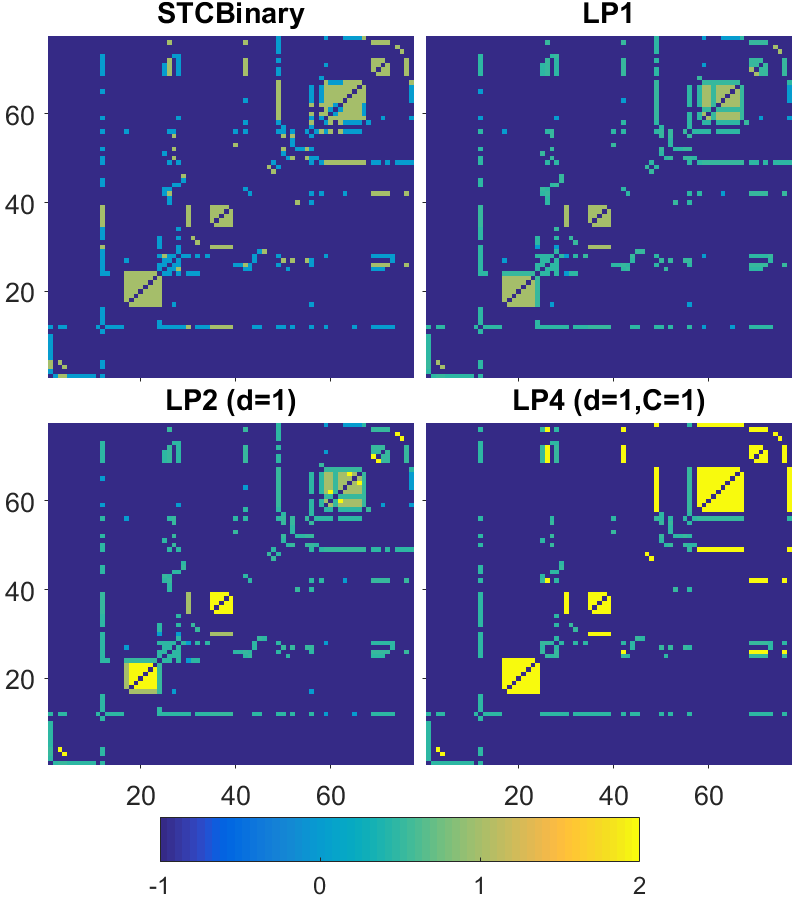
Figure 5. Heatmap of the edge strengths on Les Miserables with methods STCbinary Greedy (1st), LP1 (2nd), LP2 with $d=1$ (3rd) and LP4 with $d=1$ and $C=1$ (4th). A strength of $-1$ indicates there is no edge.

5.2. Objective performance analysis

We evaluate our approaches in a similar manner as Sintos and Tsaparas (Sintos and Tsaparas, 2014). In particular, we investigate whether the optimal strength assignments correlate to externally provided ground truth measures of tie strength, on a number of networks for which such information is available. Table 1 shows a summary of the dataset statistics and edge weight interpretations.

Table 1. Network statistics.

Network	Vertices	Edges	Edge weight meaning
Les Mis.	77	254	co-appearence of characters in same chapter
KDD	2 738	11 073	co-authorship between 2 authors
Facebook (Viswanath et al., 2009)	3 228	4 585	number of posts on each other’s wall
Twitter	4 185	5 680	mentions of each other
Authors	9 150	34 614	unknown
BitCoin OTC	5 875	21 489	Who-trust-whom score in Bitcoin OTC
BitCoin Alpha	3 775	14 120	Who-trust-whom score in Bitcoin Alpha

We compare the algorithms STCbinary Greedy (which Sintos and Tsaparas found to perform best), LP1 and LP2. For each dataset, the first row in Table 2 displays the number of edges that are assigned in that category. The second row shows the mean ground truth weight over the labeling assigned by the respective algorithm.

Les Miserables is a network where STCbinary Greedy is known to perform well (Sintos and Tsaparas, 2014). For this dataset, we can clearly see that our methods provide a correct multi-level strength labeling, enabling more refined notions of tie strength.

A second observation is that in for the networks KDD, Facebook, Twitter, and Authors, neither the existing nor the newly-proposed methods perform well. This raises the question of whether the STC assumption is valid in these networks with the provided ground truths. That said, it is reassuring to see that our methods work in a robust and fail-safe way: in such cases, as indicated by the high number of 1/2 strength assignments.

For trust networks in particular, however, it has been described that the STC property is likely to develop due to the transitive property (Easley and Kleinberg, 2010). Indeed, if a user A trusts user B and user B trusts user C, then user A has a basis for trusting user C. The two BitCoin networks are examples of such trust networks. Our methods perform well in identifying some clearly strong and some clearly weak edges, although it again takes a cautious approach in assigning an intermediate strength to many edges. Remarkably though, STCbinary Greedy performs poorly on this network, incorrectly labeling many strong edges as weak and vice versa.

Table 2. Mean ground-truth weight analysis comparison of different STC methods. For each dataset, the first row is the number of edges of an assigned label. The 2nd row indicates the mean groundtruth weight over that respective set of edges. The ground-truth strength ranges are indicated by the numbers between brackets.

Network	STCbinary Greedy			LP1				LP2 (d=1)
	1	0		1	$1/2$	0		2	1	$1/2$	0
Les Mis.	131	123		60	180	14		30	30	180	14
$[1$–$31]$	3.6	2.8		4.5	2.9	1.5		3.3	5.7	2.9	1.5
KDD	3 085	7 988		545	10 390	138		290	252	10 396	135
$[0.04$–$47.3]$	1.14	0.85		0.89	0.93	0.61		0.77	1.03	0.94	0.61
Facebook	1 451	3 134		28	4 547	10		11	17	4 547	10
$[1$–$30]$	1.9	1.94		2.29	1.92	1.5		2.46	2.18	1.92	1.5
Twitter	282	5 398		0	5 680	0		0	0	5 680	0
$[1$–$139]$	1.29	2		-	1.97	-		-	-	1.97	-
Authors	16 647	17 967		9 599	22 994	2 021		5 590	4 009	22 994	2 021
$[1$–$52]$	1.19	1.4		1.1	1.41	1.16		1.09	1.1	1.41	1.16
BitCoin OTC	1 794	19 695		37	21 446	6		26	11	21 446	6
$[-10$–$10]$	0.89	0.62		2.37	0.64	-2.33		2.5	2.1	0.64	-2.33
BitCoin Alpha	1 178	12 942		6	14 113	1		4	2	14 113	1
$[-10$–$10]$	1.21	1.43		5	1.4	-10		6	3	1.4	-10

Finally, Table 3 reports running times on a PC with an Intel i7-4800MQ CPU at 2.70GHz and 16 GB RAM of our CVX/MOSEK and Hochbaum-Naor implementations. It demonstrates the superior performance of the latter. Remarkably, the Hochbaum-Naor algorithm performs very comparably to the greedy approximation algorithm for STCbinary.

Table 3. Running times (in seconds) for solving LP2sym with $d=1$ by a general LP solver with Interior Point (IP) algorithm, for Hochbaum-Naor’s algorithm with Minimum Cut as the main subroutine, and for the greedy approximation algorithm for STCbinary. Total times include problem construction for LP2sym, graph construction for Hochbaum-Naor, and wedge-graph construction for STCbinary.

Network	LP			Hochbaum			STCbinary
	IP	total		MinCut	total		Greedy	total
Les Mis.	0.11	0.63		0.004	0.008		0.002	0.016
KDD	3.92	19.30		0.29	1.60		0.86	2.07
Facebook	0.31	1.94		0.02	0.46		0.15	0.41
Twitter	1.44	10.30		0.28	0.87		0.27	1.88
Authors	14.66	47.29		0.68	6.68		5.22	9.50
BitCoin OTC	126.22	269.31		8.69	13.41		1.54	7.12

6. Related work

This paper builds on the STC principle, which was proposed in sociology by Simmel (Simmel, 1908). Sintos and Tsaparas (Sintos and Tsaparas, 2014) first considered the problem of labeling the edges of the graph to enforce the STC property: maximize the number of strong edges, such that the network satisfies the STC property. In our work we relax and extend this formulation by introducing new constraints and integer labels. To our knowledge, we are the first to introduce and study such formulations.

The work by Sintos and Tsaparas (Sintos and Tsaparas, 2014) is part of a broader line of active recent research aiming to infer the strength of the links in a social network. E.g., Jones et al. (Jones et al., 2013) uses frequency of online interaction to predict of strength ties with high accuracy. Gilbert et al. (Gilbert and Karahalios, 2009) characterize social ties based on similarity and interaction information. Similarly, Xiang et al. (Xiang et al., 2010) estimate relationship strength from homophily principle and interaction patterns and extend the approach to heterogeneous types of relationships. Pham et al. (Pham et al., 2016) incorporate spatio-temporal features of social iterations to increase accuracy of inferred tie strength.

A related direction of research focuses solely on inferring types of the links in a network. E.g., Tang et al. (Tang et al., 2012, 2011, 2016) propose a generative statistical model, which can be used to classify heterogeneous relationships. The model relies on social theories and incorporates structural properties of the network and node attributes. Their more recent works can also produce strength of the predicted types of ties. Backstrom et al. (Backstrom and Kleinberg, 2014) focuses on the graph structure to identify a particular type of ties—romantic relationships in Facebook.

Most of these works, however, make use of various meta-data and characteristics of social interactions in the networks. In contrast, like Sintos and Tsaparas’ work, our aim is to infer strength of ties solely based of graph structure, and in particular on the STC assumption.

Another recent extension of the work of Sintos and Tsaparas (Sintos and Tsaparas, 2014) is followed by Rozenshtein et al. (Rozenshtein et al., 2017). However, their direction is different: they consider binary strong and weak labeling with additional community connectivity constrains and allow STC violations to satisfy those constraints.

7. Conclusions and further work

7.1. Conclusions

We have proposed a sequence of linear programming relaxations of the STCbinary problem introduced by Sintos and Tsaparas (Sintos and Tsaparas, 2014). These formulations have a number of advantages, most notably their computational complexity, the fact that they refrain from making arbitrary strength assignments in the presence of uncertainty, and as a result, enhanced robustness. Extensive theoretical analysis of the second relaxation (LP2) has not only provided insight into the solution and the arbitrariness the solution from STCbinary may exhibit, it also yielded a highly efficient algorithm for finding a symmetric (non-arbitrary) optimal strenght assignment.

The empirical results confirm these findings. At the same time, they raise doubts about the validity of the STC property in real-life networks, with trust networks appearing to be a notable exception.

7.2. Further work

Our research results open up a large number of avenues for further research. The first is to investigate whether more efficient algorithms can be found for inferring the range of edge strengths across the optimal face of the feasible polytope. A related research question is whether the marginal distribution of individual edge strengths, under the uniform distribution of the optimal polytope, can be characterized in a more analytical manner (instead of by uniform sampling). Both these questions seem important beyond the STC problem, and we are unaware of a definite solution to them.

A second line of research is to investigate alternative problem formulations. An obvious variation would be to take into account community structure, and the fact that the STC property probably often fails to hold for wedges that span different communities. A trivial approach would be to simply remove the constraints for such wedges, but more sophisticated approaches could exist. Additionally, it would be interesting to investigate the possibility to allow for different relationship types and respective edge strengths, requiring the STC property to hold only within each type. Furthermore, the fact that the presented formulations are LPs, combined with the fact that many graph-theoretical properties can be expressed in terms of linear constraints, opens up the possibility to impose additional constraints on the optimal strength assignments without incurring significant computational overhead as compared to the interior point implementation. One line of thought is to impose upper bounds on the sum of edge strengths incident to any given edge, modeling the well-known fact that an individual is limited in how many strong social ties they can maintain.

A third line of research is whether an active learning approach can be developed, to quickly reduce the number of edges assigned an intermediate strength by our approaches.

More directly, a fourth line of research concerns the question of whether the theoretical understanding of Problems LP1 and LP2 can be transferred more completely to Problems LP3 and LP4 than achieved in the current paper.

Finally, perhaps the most important line of further research concerns the validity of the STC property: could it be modified so as to become more widely applicable across real-life social networks?

Acknowledgements. This work was supported by the ERC under the EU’s Seventh Framework Programme (FP7/2007-2013) / ERC Grant Agreement no. 615517, FWO (project no. G091017N, G0F9816N), the EU’s Horizon 2020 research and innovation programme and the FWO under the Marie Sklodowska-Curie Grant Agreement no. 665501, three Academy of Finland projects (286211, 313927, and 317085), and the EC H2020 RIA project “SoBigData” (654024).

References

- (1)
- ApS (2015) MOSEK ApS. 2015. The MOSEK optimization toolbox for MATLAB manual. Version 7.1 (Revision 28). http://docs.mosek.com/7.1/toolbox/index.html
- Backstrom and Kleinberg (2014) Lars Backstrom and Jon Kleinberg. 2014. Romantic partnerships and the dispersion of social ties: a network analysis of relationship status on facebook. In Proceedings of the 17th ACM conference on Computer supported cooperative work & social computing. ACM, 831–841.
- Chen et al. (2017) Yuansi Chen, Raaz Dwivedi, Martin J Wainwright, and Bin Yu. 2017. Fast MCMC sampling algorithms on polytopes. arXiv preprint arXiv:1710.08165 (2017).
- Easley and Kleinberg (2010) David Easley and Jon Kleinberg. 2010. Networks, Crowds, and Markets: Reasoning About a Highly Connected World. Cambridge University Press, New York, NY, USA.
- Edelsbrunner et al. (1989) Herbert Edelsbrunner, Günter Rote, and Ermo Welzl. 1989. Testing the necklace condition for shortest tours and optimal factors in the plane. Theoretical Computer Science 66, 2 (1989), 157–180.
- Gilbert and Karahalios (2009) Eric Gilbert and Karrie Karahalios. 2009. Predicting tie strength with social media. In Proceedings of the SIGCHI conference on human factors in computing systems. ACM, 211–220.
- Grant and Boyd (2014) Michael Grant and Stephen Boyd. 2014. CVX: Matlab Software for Disciplined Convex Programming, version 2.1. http://cvxr.com/cvx. (March 2014).
- Håstad (1999) Johan Håstad. 1999. Clique is hard to approximate within . Acta Mathematica 182, 1 (1999), 105–142.
- Hochbaum (1982) Dorit S Hochbaum. 1982. Approximation algorithms for the set covering and vertex cover problems. SIAM Journal on computing 11, 3 (1982), 555–556.
- Hochbaum (1983) Dorit S Hochbaum. 1983. Efficient bounds for the stable set, vertex cover and set packing problems. Discrete Applied Mathematics 6, 3 (1983), 243–254.
- Hochbaum and Naor (1994) Dorit S Hochbaum and Joseph Naor. 1994. Simple and fast algorithms for linear and integer programs with two variables per inequality. SIAM J. Comput. 23, 6 (1994), 1179–1192.
- Jones et al. (2013) Jason J Jones, Jaime E Settle, Robert M Bond, Christopher J Fariss, Cameron Marlow, and James H Fowler. 2013. Inferring tie strength from online directed behavior. PloS one 8, 1 (2013), e52168.
- Mehrotra and Ye (1993) Sanjay Mehrotra and Yinyu Ye. 1993. Finding an interior point in the optimal face of linear programs. Mathematical Programming 62, 1 (1993), 497–515.
- Nemhauser and Trotter (1975) George L Nemhauser and Leslie Earl Trotter. 1975. Vertex packings: structural properties and algorithms. Mathematical Programming 8, 1 (1975), 232–248.
- Pham et al. (2016) Huy Pham, Cyrus Shahabi, and Yan Liu. 2016. Inferring social strength from spatiotemporal data. ACM Transactions on Database Systems (TODS) 41, 1 (2016), 7.
- Rozenshtein et al. (2017) Polina Rozenshtein, Nikolaj Tatti, and Aristides Gionis. 2017. Inferring the Strength of Social Ties: A Community-Driven Approach. In Proceedings of the 23rd ACM SIGKDD International Conference on Knowledge Discovery and Data Mining. ACM, 1017–1025.
- Simmel (1908) Georg Simmel. 1908. Soziologie Untersuchungen über die Formen der Vergesellschaftung.
- Sintos and Tsaparas (2014) Stavros Sintos and Panayiotis Tsaparas. 2014. Using strong triadic closure to characterize ties in social networks. In Proceedings of the 20th ACM SIGKDD international conference on Knowledge discovery and data mining. ACM, 1466–1475.
- Spielman and Teng (2004) Daniel A Spielman and Shang-Hua Teng. 2004. Smoothed analysis of algorithms: Why the simplex algorithm usually takes polynomial time. Journal of the ACM (JACM) 51, 3 (2004), 385–463.
- Tang et al. (2012) Jie Tang, Tiancheng Lou, and Jon Kleinberg. 2012. Inferring social ties across heterogenous networks. In Proceedings of the fifth ACM international conference on Web search and data mining. ACM, 743–752.
- Tang et al. (2016) Jie Tang, Tiancheng Lou, Jon Kleinberg, and Sen Wu. 2016. Transfer learning to infer social ties across heterogeneous networks. ACM Transactions on Information Systems (TOIS) 34, 2 (2016), 7.
- Tang et al. (2011) Wenbin Tang, Honglei Zhuang, and Jie Tang. 2011. Learning to infer social ties in large networks. In Joint European Conference on Machine Learning and Knowledge Discovery in Databases. Springer, 381–397.
- Viswanath et al. (2009) Bimal Viswanath, Alan Mislove, Meeyoung Cha, and Krishna P. Gummadi. 2009. On the Evolution of User Interaction in Facebook. In Proceedings of the 2nd ACM SIGCOMM Workshop on Social Networks (WOSN’09).
- Xiang et al. (2010) Rongjing Xiang, Jennifer Neville, and Monica Rogati. 2010. Modeling relationship strength in online social networks. In Proceedings of the 19th international conference on World wide web. ACM, 981–990.