Constructing first-principles phase diagrams of amorphous Li_xSi using machine-learning-assisted sampling with an evolutionary algorithm

Abstract

The atomistic modeling of amorphous materials requires structure sizes and sampling statistics that are challenging to achieve with first-principles methods. Here, we propose a methodology to speed up the sampling of amorphous and disordered materials using a combination of a genetic algorithm and a specialized machine-learning potential based on artificial neural networks (ANN). We show for the example of the amorphous LiSi alloy that around 1,000 first-principles calculations are sufficient for the ANN-potential assisted sampling of low-energy atomic configurations in the entire amorphous Li_xSi phase space. The obtained phase diagram is validated by comparison with the results from an extensive sampling of Li_xSi configurations using molecular dynamics simulations and a general ANN potential trained to $\sim$45,000 first-principles calculations. This demonstrates the utility of the approach for the first-principles modeling of amorphous materials.

I Introduction

Amorphous phases determine the properties of many technologically relevant materials, such as catalysts for water oxidation and reduction,Chemelewski et al. (2014); Gu et al. (2015); Morales-Guio et al. (2014) lithium and sodium ion battery electrodes,McDowell et al. (2013); Qian et al. (2013) electrodes for solid oxide fuel cells,Evans et al. (2015); Song et al. (2017) and the solid electrolyte interphase at the electrode/electrolyte boundary.Sacci et al. (2015) Owing to the absence of long-range order, amorphous structures cannot be characterized by conventional diffraction techniques. Other characterization methods, such as X-ray or neutron pair distribution function measurements, only provide indirect structural information. First principles density-functional theory (DFT) Hohenberg and Kohn (1964); Kohn and Sham (1965); Burke (2012) offers predictive insight into phase stabilities and structures Urban et al. (2016) and is an attractive alternative for the characterization of atomic structures and their properties. However, the high computational cost of DFT calculations confines the method to structure models containing at most a few hundred atoms and moderate sampling, a limitation that in practice makes it challenging to model many amorphous or disordered phases.

To overcome these sampling and size limitations, recently a number of machine-learning techniques have been proposed that can be used to efficiently interpolate first principles energies and atomic forces.Behler and Parrinello (2007); Bartók et al. (2010); Rupp et al. (2012); Faber et al. (2016); Morawietz et al. (2016); Brockherde et al. (2017) Machine-learning potentials (MLPs) have enabled large-scale simulations of complex materials such as nanoalloys, Artrith and Kolpak (2014, 2015) metal-oxide nanoparticles, Elias et al. (2016) and amorphous carbon Deringer and Csányi (2017) with an accuracy that is close to the reference method, but at a fraction of the computational cost. However, to reliably sample all relevant atomic interactions MLPs have to be trained on extensive databases of first-principles calculations. Depending on the number of chemical species, several thousand to tens of thousands of reference data points might be required to obtain a reliable MLP. By their nature, amorphous phases exhibit a large variety of local structural motifs, making the compilation of complete structural reference databases even more challenging.

Here we propose an alternative approach for the calculation of first-principles phase diagrams of amorphous materials with machine-learning-assisted sampling. Instead of constructing a general MLP based on tens of thousands of reference calculations, we employ a specialized MLP trained on only around one thousand DFT calculations of small structures, and which is used specifically for the sampling of near-ground-state structures with a genetic algorithm. The relevant structures identified by this sampling approach are recomputed using DFT to obtain an accurate first-principles phase diagram. Finally, we validate the approximate sampling approach by training a fully converged general MLP that makes possible extensive molecular dynamics simulations.

We consider Li_xSi alloys as a prototypical example of an amorphous electrode material. Nanostructured amorphous Si is a potential high-capacity negative electrode material for Li-ion batteries.McDowell et al. (2013); Su et al. (2013); Zamfir et al. (2013); Wang et al. (2016) The lithiation of crystalline Si has previously been studied with first-principles calculations on small model structures, and through mesoscale simulation techniques.Chevrier and Dahn (2009); Chevrier et al. (2009); Chevrier and Dahn (2010); Wan et al. (2010); Kim et al. (2011); Chan et al. (2011); Cubuk et al. (2013); Chan et al. (2012); Cubuk and Kaxiras (2014); Jung et al. (2015); Ostadhossein et al. (2015) In the present article, we consider significantly larger structure models with more than 600 atoms, which provides additional insight into the energetics of the amorphous LiSi phase.

The paper is structured as follows: In section II, we detail all simulation parameters and recap the artificial neural network potential method, as well as the descriptor technique used to capture the local atomic environment. This is followed by a description of the construction of the specialized MLP and the genetic algorithm in section III and the molecular dynamics sampling in section IV. In the next section IV.2, the phase space of amorphous Li_xSi structures that is sampled by the genetic algorithm is compared with that of the molecular dynamics heat-quench simulations. The results are assessed in a final discussion section V.

II Energy Models

II.1 Density-functional theory calculations

All density-functional theory (DFT) calculations were carried out using the Vienna Ab-Initio Simulation Package (VASP).Kresse and Furthmüller (1996a, b) The exchange-correlation functional by Perdew, Burke, and Ernzerhof (PBE) Perdew et al. (1996, 1997) and projector-augmented wave (PAW) pseudopotentials Blöchl (1994) were used. The energy cutoff of the plane wave basis set was generally 520 eV, and a $k$-point density of 1000 divided by the number of atoms was used for the Brillouin-zone integration following the recommendations from reference 42. VASP input files were generated using the Python Materials Genomics tool (pymatgen).Ong et al. (2013) In geometry optimizations, energies were generally converged to 0.05 meV/atom and the convergence thresholds for atomic forces was 50 meV/Å.

II.2 Machine-learning potentials with Chebyshev descriptor

The idea behind machine-learning potentials (MLPs) is to interpolate first principles potential energies and atomic forces using machine learning techniques, such as artificial neural networks (ANNs) Behler and Parrinello (2007); Rupp et al. (2012) or Gaussian process regression.Bartók et al. (2010) For the structure space that it is trained on, an MLP can be nearly as accurate as its reference method at a fraction of the computational cost.Behler (2017) Several approaches in this spirit have been proposed, varying in the details of the machine learning model, the atomic structure descriptor, and the interpolated quantity (total energy vs. atomic energy).Bartók and Csányi (2015); Ghasemi et al. (2015); De et al. (2016); Faber et al. (2016)

In the present work, we employ ANNs to interpolate the atomic energy from DFT calculations, and the total energy of an atomic structure $\sigma$ is given as the sum of the atomic energies of all atoms

$$E(\sigma)=\sum_{i}^{N_{\textup{atoms}}}E_{\textup{atom}}(\sigma_{i}^{R_{c}})\quad.$$ (1)

In equation (1), $\sigma_{i}^{R_{c}}=\{\vec{R}_{j},t_{j}:||\vec{R}_{j}-\vec{R}_{i}||\leq{}R_{c}\}$ captures the local atomic environment of atom $i$, i.e., the set of the coordinates $\vec{R}_{j}$ and chemical species $t_{j}$ of atoms within a radial cutoff $R_{c}$ from atom $i$. Note that the number of atoms in $\sigma_{i}^{R_{c}}$ (i.e., within the cutoff radius) depends directly on the density of the structure, and the number of chemical species additionally depends on the chemical composition.

For the construction of a transferable ANN potential, a constant-size descriptor of the local atomic environment is needed (see section II.2.1). With such a descriptor of the local atomic environment, $\widetilde{\sigma}_{i}^{R_{c}}$, the total energy of the ANN potential is then given by

$$E(\sigma)=\sum_{i}^{N_{\textup{atoms}}}\textup{ANN}_{t_{i}}(\widetilde{\sigma}_{i}^{R_{c}})\quad,$$ (2)

where $\textup{ANN}_{t_{i}}$ is the atomic energy ANN potential for chemical species $t_{i}$.

In the present work, an ANN architecture with two hidden layers each consisting of 15 nodes was used, giving a descriptor dimension of 44 (see section II.2.1) and a total of 931 ANN parameters. We previously confirmed that this architecture provides sufficient flexibility to fit high-dimensional first principles data.Artrith and Behler (2012); Artrith et al. (2013); Artrith and Kolpak (2014)

Before the ANN potential training, ten percent of all reference data points were randomly selected as an independent test set for cross-validation and were not considered during training. The ANN potentials were trained using the limited-memory Broyden-Fletcher-Goldfarb-Shanno (L-BFGS) method Byrd et al. (1995); Zhu et al. (1997) as implemented in the atomic energy network (ænet) package.Artrith and Urban (2016) Training was repeated ten times using different randomly initialized fitting parameters, and out of this set the optimal ANN fit was selected.

II.2.1 Descriptor of the local atomic environment

The atomic coordinates cannot directly be used as ANN input, as the number of atoms within the interaction range $R_{c}$ varies with the structure and density of the material. Hence, a descriptor of the local atomic environment with constant dimension is required as the input layer of the atomic energy ANN model in Eq.(2). The descriptor additionally has to obey the invariants of the atomic energy, i.e., it has to be invariant with respect to rotation, translation, and the exchange of equivalent atoms. Several atomic structure descriptors for machine-learning models have been proposed in the literature.Behler (2011); Sadeghi et al. (2013); Bartók et al. (2013); Schütt et al. (2014); Faber et al. (2015); von Lilienfeld et al. (2015); Huo and Rupp (2017)

Here we employ a recently developed descriptor based on the expansion of the radial and angular distribution functions (RDF and ADF) that is numerically efficient and has the advantage that its complexity does not increase with the number of chemical species.Artrith et al. (2017) A complete dervation and benchmarks of the method can be found in the original reference 60. In brief, the RDF and ADF of the local structural environment of atom $i$ within a cutoff radius $R_{c}$ are defined as

$$\mathrm{RDF}_{i}(r) =\sum_{\mathclap{\;\;\mathbf{R}_{j}\in\,\sigma_{i}^{R_{\textup{c}}}}}\delta(r-R_{ij})\,f_{\textup{c}}(R_{ij})\,w_{t_{j}}$$ (3)

$$\mathrm{ADF}_{i}(\theta) =\sum_{\mathclap{\;\;\mathbf{R}_{j},\mathbf{R}_{k}\in\,\sigma_{i}^{R_{\textup{c}}}}}\delta(\theta-\theta_{ijk})\,f_{\textup{c}}(R_{ij})\,f_{\textup{c}}(R_{ik})\,w_{t_{j}}w_{t_{k}}\quad,$$ (4)

where $R_{ij}$ is the bond distance between atoms $i$ and $j$, $\theta_{ijk}$ is the bond angle for atoms $i$, $j$, and $k$, and

$$f_{\textup{c}}(r)=\begin{cases}\frac{1}{2}\Bigl{[}\cos\Bigl{(}r\cdot\frac{\pi}{R_{\textup{c}}}\Bigr{)}+1\Bigr{]}&\text{for}\quad r\leq{}R_{c}\\ 0&\text{else}\end{cases}$$ (5)

is a cutoff function. The choice of the weights $w_{t_{i}}$ for chemical species $t_{i}$ will be discussed shortly. Both RDF and ADF automatically obey the invariants of the atomic energy. Expanding the RDF and ADF in an orthonormal basis set, up to a specified order $N$, gives an approximate constant-size representation that can be used as a descriptor for a machine-learning model.

With a basis set of Chebyshev polynomials $\{T_{\alpha}\}$, the following expressions are obtained for the expansion coefficients of the RDF

$$\begin{aligned} c^{(2)}_{\alpha}&=\sum_{\mathclap{\;\;\mathbf{R}_{j}\in\,\sigma_{i}^{R_{\textup{c}}}}}T_{\alpha}\Bigl{(}\frac{2R_{ij}}{R_{\textup{c}}}-1\Bigr{)}\,f_{\textup{c}}(R_{ij})\,w_{t_{j}}\\ &\hskip 86.11084pt\text{with}\quad 0\leq R_{ij}\leq R_{c}\end{aligned}$$ (6)

and the ADF

$$\begin{aligned} c^{(3)}_{\alpha}&=\sum_{\mathclap{\;\;\mathbf{R}_{j},\mathbf{R}_{k}\in\,\sigma_{i}^{R_{\textup{c}}}}}T_{\alpha}\Bigl{(}\frac{2\theta_{ijk}}{\pi}-1\Bigr{)}\,f_{\textup{c}}(R_{ij})\,f_{\textup{c}}(R_{ik})\,w_{t_{j}}w_{t_{k}}\\ &\hskip 86.11084pt\text{with}\quad 0\leq\theta_{ijk}\leq\pi\quad.\end{aligned}$$ (7)

Note that the arguments of $T_{\alpha}$ in Eqs. (6) and (7) are scaled to the interval $[-1.0,+1.0]$ for which the Chebyshev polynomials are orthogonal with

$$\int_{-1}^{1}\!\!\!T_{n}(x)T_{m}(x)\frac{\mathrm{d}x}{\sqrt{1-x^{2}}}=\begin{cases}\pi&n=m=0\\ \frac{\pi}{2}&n=m\neq{}0\\ 0&\text{else}\end{cases}$$ (8)

$$\quad\text{for}\quad x\in{}[-1.0,+1.0]\quad.$$

To construct a descriptor for both the local atomic structure $\{\vec{R}_{i}\}$ and the chemical species $\{t_{i}\}$, two sets of expansion coefficients are used: The first set only describes the local structure, and all species weights $w_{t_{i}}$ in Eqs. (1) through (7) are taken to be equal to 1, i.e., all atomic species are considered to be equivalent in the expansion. Expanding the RDF and ADF with this choice of $w_{t_{i}}$ yields the coefficients $\{{}^{\textup{s}}c_{\alpha}^{(2)},{}^{\textup{s}}c_{\alpha}^{(3)}\}$ which describe only structural features. The second set of coefficients is obtained by assigning a different value $w_{t_{i}}$ to each chemical species $t_{i}$, yielding the expansion coefficients $\{{}^{\textup{t}}c_{\alpha}^{(2)},{}^{\textup{t}}c_{\alpha}^{(3)}\}$ that describe the atom types. The combined set $\{{}^{\textup{s}}c_{\alpha}^{(2)},{}^{\textup{s}}c_{\alpha}^{(3)},{}^{\textup{t}}c_{\alpha}^{(2)},{}^{\textup{t}}c_{\alpha}^{(3)}\}$ is used as the descriptor for the ANN potentials. One possible choice of unique species weights for compositions with $N_{t}$ chemical species is $w_{t_{i}}=(0,)\pm{}1,\pm{}2,\ldots,\lfloor{}\frac{N_{t}}{2}\rfloor$ where $0$ is only included for odd numbers of species. Artrith et al. (2017)

For the present work, we choose $w_{\textup{Li}}$ = -1 and $w_{\textup{Si}}$ = +1, and $N=11$ Chebyshev polynomials are used for both the radial and angular expansions. Hence, the combined descriptor with radial and angular coefficients for structure and atomic species has a total dimension of $4\times{}11=44$.

III Genetic algorithm sampling with a specialized ANN potential

The stable ground state phases of the LiSi alloy and their crystalline structures, c-Li8Si8,Stearns et al. (2003) c-Li12Si7,Nesper et al. (1986) c-Li7Si3,Schnering et al. (1980) c-Li13Si4,Frank et al. (2014) and c-Li21Si5,Nesper and von Schnering (1987) are well known.Wen and Huggins (1981); Chevrier et al. (2010) However, during lithiation and delithiation at room temperature these crystalline phases are not observed. Instead, metastable amorphous a-Li_xSi structures form that crystallize into the metastable c-Li15Si4 phaseLimthongkul et al. (2003); Hatchard and Dahn (2004); Obrovac and Christensen (2004); Li and Dahn (2007); McDowell et al. (2013) when the Li potential drops to $\sim$50 mV vs. Li+/Li

To generate realistic amorphous LiSi structures as they occur in an actual Li-ion battery anode, we directly simulate the amorphization during electrochemical delithiation. This means, Li is computationally extracted from the fully lithiated and crystalline Li15Si4 structure and the atomic positions and the cell parameters are relaxed at intermediate compositions.

III.1 A specialized ANN potential for the sampling of near-ground-state Li_xSi structures

To determine the structure of the metastable amorphous Li_xSi phase at different compositions, we employ an evolutionary (or genetic) algorithm for the sampling of Li/vacancy orderings coupled with a specialized ANN potential.

To train a suitable ANN potential, an initial set of Li_xSi reference structures was generated by isotropic scaling of the lattice parameters by up to $\pm{}5\%$ and by distortion of the crystalline c-Li_xSi phases, structures of which were obtained from the Materials Project database.Jain et al. (2013) In addition to the ideal crystal structures, structures with random Li and Si vacancies were also included. The resulting initial reference set comprised 725 Li_xSi structures and was used to train a specialized ANN potential for the GA sampling.

We consider this potential to be specialized because it is trained only to DFT reference calculations of structures that are related to the crystalline Li_xSi structures. As such, it cannot be expected that the resulting potential would reproduce the correct energetics of structural motifs that are very different from those of the crystalline structures, such as different atomic coordinations and much shorter bond length, as they would occur at very high energies. However, we hypothesize that the specialized potential is suitable for the specific purpose of sampling near-ground-state Li/vacancy arrangements in delithiated amorphous Li_15-xSi4 structures.

III.2 Sampling amorphous Li_xSi structures with a genetic algorithm

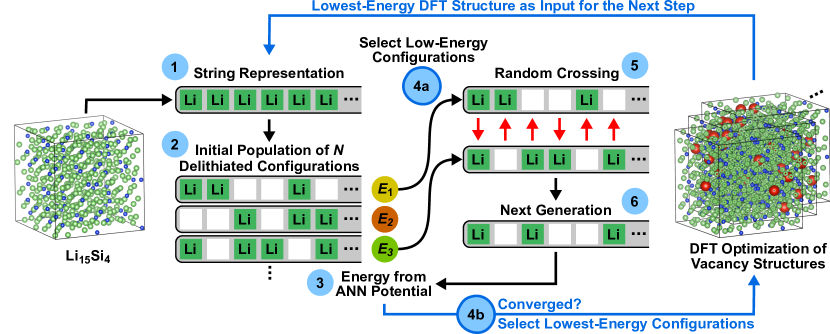
Figure 1: Schematic of the genetic algorithm (GA) sampling approach using the specialized ANN potential. The GA is used to identify the most likely Li atoms to be extracted at each delithiation step, starting with the crystalline Li15Si4 structure. The atomic positions and cell parameters of configurations with intermediate compositions are subsequently optimized using DFT. The magnitude of the energies shown in the schematic are $E_{3}<E_{1}<E_{2}$. Li atoms are shown as green balls, Si is blue, and vacancies are red. See text for details of the algorithm.

Genetic algorithms (GAs) are standard global optimization techniques Goldberg (1989) and have been routinely applied to atomic structure optimization problems.Deaven and Ho (1995); Oganov and Glass (2006); Abraham and Probert (2006); Hajinazar et al. (2017) Here, we are dealing with a simplified optimization problem in that we only seek to identify those Li atoms that are most likely to be removed at each delithiation step. The specific delithiation algorithm employed in the present work is as follows: (i) The GA is used to determine the most stable Li/vacancy configuration for a supercell of the Li_15-xSi_4 structure. (ii) The atomic coordinates and lattice parameters of at least the 30 most stable configurations as predicted by the GA are optimized with DFT. (iii) The most stable (lowest-energy) structure as determined by DFT is used as the starting point for the next delithiation step, and the scheme is continued with step (i).

A schematic of the GA method used in the present work is shown in Fig. 1. In detail, the GA involves the following individual steps:

1. Input for the GA is the structure of one particular Li_xSi composition. For the first delithiation step, a supercell of the ideal Li15Si4 structure is used.

2. The atomic configuration is represented as a vector (or string) in which only Li sites are considered;

3. An initial population of $N$ trial configurations is generated by randomly removing Li atoms from the input structure (delithiation) to realize the specific Li_x₁Si composition of the present delithiation step;

4. The energy of each trial configuration is evaluated using the ANN potential. If the optimization has converged and no lower energy was determined over a certain number of steps the algorithm is continued with step 4b, else the optimization is continued with step 4a;

5. For the following steps, each two trial configurations from the current population are selected with probabilities that are proportional to their energy such that lower energy means higher selection probability. This selection method is sometimes called roulette wheel selection; Goldberg (1989)

6. $N$ additional trials are generated by combination (crossing) of two selected trials from the current population. Each new trial configuration is further subject to random changes with a mutation probability of $p_{m}$ (not shown in Fig. 1);

7. The energies of the new trial configurations are evaluated using the ANN potential, and the algorithm continues with step 3;

8. Once the GA optimization has converged or a set number of steps have been completed, the $M$ configurations with the lowest energies are prepared for subsequent geometry optimizations with DFT.

For the present work, we used a population size of $N$ = 32 trials and a mutation rate of $p_{m}$ = 10%. At least $M=30$ configurations were optimized with DFT at each composition. A Python implementation of the above GA algorithm can be obtained from http://ga.ann.atomistic.net.

Using the GA approach described above coupled with the specialized ANN potential of section III.1, two different supercells of the c-Li15Si4 phase with compositions Li60Si16 (76 atoms) and Li480Si128 (608 atoms) were delithiated. The small Li60Si16 cell was delithiated in intervals of each 2 Li atoms, and the large Li480Si128 cell was delithiated in steps of 8 Li atoms.

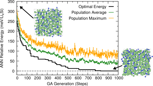
Figure 2: Energy of the Li360Si128 configurations during optimization with the genetic algorithm (GA) coupled with the specialized ANN potential. The energy of the current best configuration is shown as black line (optimal energy), the green line corresponds to the average energy of the GA population of 32 trials, and the yellow line is the current maximal energy. The insets show the initial structure and the final structure with lowest energy after optimization with DFT. Li and Si atoms are colored green and blue, respectively.

As one concrete example, the course of the energy during GA optimization of an atomic configuration with composition Li360Si128 is shown in Fig. 2. As seen in the figure, after around 500 GA steps the energy only changes by around 13 meV/Li_xSi, indicating that the optimization has reasonably converged.

A total of 1,263 structures from this GA sampling were selected for subsequent DFT evaluation and geometry optimization, and together with the initial reference set they form the basis for the first principles phase diagram discussed below.

IV Molecular dynamics sampling with a general ANN potential

The GA methodology described above makes two approximations that may intuitively not seem justified: (i) The GA sampling does not consider structural relaxations (though, the final 30 or more low-energy configurations are fully optimized), and (ii) the ANN potential is specialized for the GA sampling and would not be suitable for other applications. To verify that the GA sampling generated genuinely low-energy metastable amorphous structures, we compare the resulting phase diagram with the one obtained from heat-quench molecular dynamics (MD) simulations.

All MD simulations were carried out using the Tinker software package Ponder and Richards (1987) and a Parrinello-Bussi thermostat Bussi et al. (2007) in the $NVT$ ensemble. Generally, a time step of 2 fs was used for the integration of the equation of motion with the Verlet algorithm.Verlet (1967)

IV.1 ANN potential construction and molecular dynamics simulations

To carry out reliable MD simulations, a fully general ANN potential is required. For the training of such an ANN potential, a more extensive set of DFT reference calculations is needed that also includes local structural motifs that do not occur in near-ground-state bulk structures. This means, also unphysical bonding situations and lattice parameters as well as unusual coordinations should be present in the reference data set, so that structures that exhibit those features are not artificially overstabilized during MD simulations. Therefore, we also included clusters with up to $\approx$200 atoms, and surface slab structures that were truncated from the bulk in addition to further bulk reference structures.

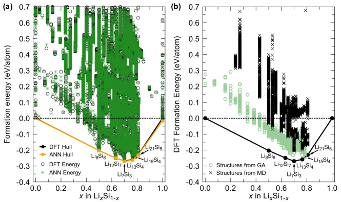
Figure 3: (a) Phase diagram based on the formation energies of all $\sim$45,000 Li_xSi structures including bulk, surface slab, and cluster structures from both training and test set. The energies predicted by the general ANN potential are shown as green stars and the DFT reference energies are black circles. (b) Only DFT formation energies of those structures sampled by the GA with the specialized ANN potential (green circles) and only those generated during MD simulations with the general ANN potential (black crosses).

The additional structures were generated by repeated MD simulations. In addition to the crystalline Li_xSi structures, the lowest energy structures from the GA sampling of section III.2 were also used as starting points for MD simulations. Hence, structures with up to 608 atoms were considered.

Short (< 10 ps) ANN potential MD simulations of the input Li_xSi structures at very high temperatures up to 3,000 K were employed to amorphize the structures. These heating simulations were followed by subsequent 2 ns long simulations at lower temperatures (between 400 K and 1200 K) to obtain equilibrated low-energy structures. 400 structures (every 5 ps) along each 2 ns long MD trajectory were recomputed with DFT single-point calculations and subsequently included in the reference data set.

MD simulations and ANN potential re-training were repeated until a low root mean squared error (RMSE) relative to the DFT energies was obtained and all Li_xSi ground states of the ANN potential and DFT energies were in agreement. Iterative ANN potential training based on MD simulations is also described in more detail in reference 52.

In total, around 45,000 reference structures were used for the training of the general ANN potential, including the reference structures of the specialized potential, the structures from GA sampling, and the additionally generated bulk, slab, and cluster structures. Ten percent of this reference data set, around 4,500 randomly selected structures, were set aside as an independent test set for cross validation and were not used in the final ANN potential training. Simultaneously, 10 different ANN potentials were trained with different random initial ANN weight parameters on the remaining 40,500 data points. Out of these potentials, the one with the smallest overall error relative to the DFT reference energies reproduces the DFT ground state phase diagram most accurately and was therefore selected for the subsequent analysis.

The selected ANN potential achieves an RMSE of 7.7 meV/atom and a mean absolute error (MAE) of 5.9 meV/atom for the test set. The RMSE and MAE for the training set are 6.3 and 5.7 meV/atom, respectively.

Figure 3a shows a comparison of the formation energies predicted by the ANN potential and their DFT references for all structures in the reference data set. As seen in the figure, all features of the DFT formation energies are correctly reproduced by the ANN potential, and the energies of the individual data points are in good agreement. In the present work, this general ANN potential is only used for the purpose of validating the results of the approximate GA sampling. However, this general potential will enable the investigation of other properties of the LiSi alloy in future projects.

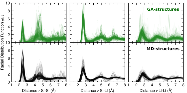
Figure 4: Superposition of the radial distribution functions (RDF) of each 1,000 randomly selected structures obtained from the GA sampling (top) and from the MD sampling (bottom).

IV.2 Comparison of the amorphous phase space sampled by GA and MD

Having at hand the two sets of independently sampled amorphous Li_xSi structures from the approximate GA sampling (section III.2) and from the extensive MD heat-quench sampling (section IV.1), we can now directly assess the differences. Figure 3b shows only those DFT formation energies belonging to structures obtained from the GA sampling (light green circles) and from the MD sampling (black crosses). Clearly, the GA sampling yielded consistently lower energy structures than the MD sampling at all considered Li_xSi compositions. Despite the approximations made in the GA sampling, the sampled structures are within a small energy range of around 100 meV/atom above the lowest energy of all a-Li_xSi for each composition. Thus, the ANN-potential-assisted GA sampling is successful in determining structure models of low-energy metastable amorphous phases, and a fully converged and general ANN potential is not required if that is the only objective.

V Discussion

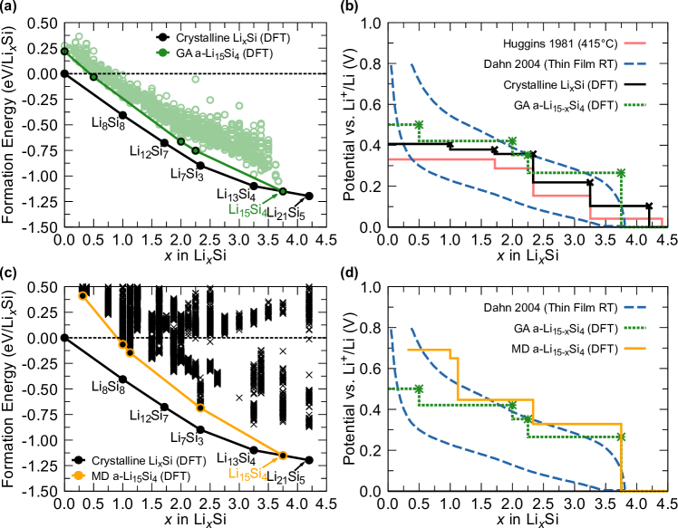
Figure 5: (a) DFT formation energies of the amorphous Li_480-xSi128 structures generated by the GA sampling (green) along with the convex hull of the crystalline LiSi phases. In this figure, the composition axis has been normalized to a constant Si content (Li_xSi) which reflects the Li storage capacity per Si atom in a Si anode. (b) Computed voltages corresponding to the lower convex hulls of the formation energies in (a) compared to measured voltage profiles from the literature. The DFT voltage profile based on the crystalline Li_xSi phases (black solid line) can be compared to the equilibrium voltages measured by Huggins et al.Wen and Huggins (1981) (light red line), while the DFT voltages of the amorphous phases (dotted green line) more closely correspond to the voltage profile by Dahn et al.Hatchard and Dahn (2004) (dashed blue line) measured for a thin film amorphous Si anode. (c) DFT formation energies of the structures from MD sampling. (d) Comparison of the computed amorphous Li_xSi voltage profiles based on the GA and MD structures.

The coupling of a GA with a specialized MLP (GA-MLP) as proposed in this work is designed to generate low-energy metastable amorphous structures, and we demonstrated that this is accomplished. However, the comparison of the GA and MD sampling results in the previous section show that the sampling strategy has a pronounced effect on the structures and energetics. In our simulations, computationally quenching a melt gives rise to energetically quite different results than computational delithiation. It should be noted that the outcome of the heat-quench simulations depends on the cooling rate of the quenching step and on the simulated time scale, as rapid quenching can trap the system in high-energy states. However, the 2 ns long MD simulations of the present work are already far beyond the time scales that can be reached with first principles methods. In practice, it depends on the concrete application which sampling strategy is most appropriate to model an amorphous phase. When modeling glasses, for example, heat-quench simulations may be most appropriate. In the present example of electrochemical amorphization, simulated delithiation more closely resembles the actual mechanism.

To better understand the differences between the structures generated by the two different sampling approaches, we evaluated the radial pair distribution functions (RDFs) for each 1,000 structures from the GA and MD sampling. A superposition of the RDFs is shown in Fig. 4. As seen in the figure, the majority of structures generated by the MD heat-quench simulations exhibit little correlations beyond the first coordination shell, and at a distance of 8 Å the RDFs approach a value of 1 indicating absence of ordering. In contrast, the structures generated using the GA sampling approach exhibit stronger long-range correlations reminiscent of the ground-state crystal structures as can be seen by comparison with the RDFs reported by Dahn et al. for the crystalline LiSi phases.Chevrier and Dahn (2009) The reason for this difference is likely that the heat-quench simulations start at high temperatures at which no long-range ordering is present, and the cooling-rate is apparently too fast to allow for the emergence of ordering. The GA sampling, on the other hand, simulates the amorphization by lithium extraction without temperature effects.

One concrete example related to the Li_xSi alloy is the voltage relative to Li+/Li. Computationally, the average conversion voltage between two Li_xSi phases at $T$ = 0 K can be well approximated based on the first-principles energy differences relative to Li metal Aydinol et al. (1997); Urban et al. (2016)

$$\overline{V}=-\frac{E(\ce{Li_{x_{1}}Si})-E(\ce{Li_{x_{2}}Si})-(x_{1}-x_{2})E(\ce{Li})}{(x_{1}-x_{2})F}$$ (9)

$$\quad\text{with}\quad x_{1}>x_{2}\quad,$$

where $F$ is Faraday’s constant. In Eq. 9, the energies E(Li_xSi_y) are obtained from the lower convex hull of the formation energy which corresponds to the T = 0 K phase diagram. At higher temperatures, the steps of the voltage profile will be smoothed out to some extend.der Ven and Ceder (2004) Figure 5a shows the formation energies of the structures from GA sampling for a lithium content that is normalized to one Si atom, so that the $x$-axis corresponds directly to the capacity in battery applications. The corresponding computational 0 K voltage profiles for the crystalline and amorphous phases are shown in Fig. 5b along with experimentally measured voltage profiles taken from the literature.Wen and Huggins (1981); Hatchard and Dahn (2004) Note that the T = 0 K voltage profile of the crystalline LiSi phases (solid black line in Fig. 5b) agrees well with the measured T = $415^{\circ}$C voltage profile showing that the 0 K voltage profile is a reasonable approximation. The formation energies and voltage profile from MD sampling are equivalently visualized in Fig. 5c and Fig. 5d. Evidently, the GA-generated formation energies shown in Fig. 5a give rise to a qualitatively and quantitatively different 0 K phase diagram as those from the MD sampling (Fig. 5c), as defined by the lower convex hull of the formation energies. The higher energies of the structures from MD sampling for low Li contents and the overall greater slope of the convex hull result in a much steeper voltage profile than the GA counterpart, as seen in Fig. 5d. The large hysteresis in the experimental voltage profile prevents a quantitative comparison with the computed voltages, though the voltage profile based on the energetics from GA sampling is closer to the experimental average.

Finally, we stress that machine-learning-assisted sampling is neither limited to the present application (delithiation) nor to genetic algorithms. The main message of the present work is instead that a specialized machine-learning potential is sufficient for structural sampling in a limited domain. Other amorphization mechanisms, such as amorphization caused by off-stoichiometries (e.g., from doping) can be modeled with an equivalent sampling setup. As an alternative to a GA for the sampling of low-energy configurations, we could have also employed other techniques such as Monte-Carlo simulations (i.e., simulated annealing).Artrith and Kolpak (2014) It should be noted that the GA sampling does not describe real-time dynamics and the present methodology assumes quasi-equilibration at each composition. The obtained voltages therefore correspond to equilibrium voltages, i.e., slow delithiation. In contrast, the MD sampling corresponds to a delithiation rate that is determined by the length of the simulated trajectories between delithiation steps (2 ns) which might provide an explanation of the higher voltages obtained from the MD sampling.

VI Conclusions

Using the example of the amorphous LiSi alloy, we showed how specialized machine-learning potentials can be used to speed up the first-principles sampling of complex structure spaces. Our methodology is based on a combination of a genetic algorithm (GA) with an artificial neural network (ANN) potential. We demonstrated that this ANN-assisted sampling is successful in determining low-energy amorphous structures and is computationally more efficient than the construction of a converged general ANN potential. Using molecular dynamics heat-quench simulations, we confirmed that the metastable structures generated by ANN-assisted GA sampling are consistently within a low energy range. The herein described method is not limited to a specific material or amorphization mechanism but is generally applicable to the modeling of amorphous and disordered materials.

VII Acknowledgments

The authors thank China Automotive Battery Research Institute Co., Ltd. and General Research Institute for NonFerrous Metals (GRINM) for financial support. This work used the computational facilities of the Extreme Science and Engineering Discovery Environment (XSEDE), which is supported by National Science Foundation grant no. ACI-1053575. Additional computational resources from the University of California Berkeley, HPC Cluster (SAVIO) are also gratefully acknowledged.

References

- Chemelewski et al. (2014) W. D. Chemelewski, H.-C. Lee, J.-F. Lin, A. J. Bard, and C. B. Mullins, J. Am. Chem. Soc. 136, 2843 (2014).
- Gu et al. (2015) J. Gu, Y. Yan, J. L. Young, K. X. Steirer, N. R. Neale, and J. A. Turner, Nat. Mater. 15, 456 (2015).
- Morales-Guio et al. (2014) C. G. Morales-Guio, S. D. Tilley, H. Vrubel, M. Grätzel, and X. Hu, Nat. Commun. 5, 3059 (2014).
- McDowell et al. (2013) M. T. McDowell, S. W. Lee, W. D. Nix, and Y. Cui, Adv. Mater. 25, 4966 (2013).
- Qian et al. (2013) J. Qian, X. Wu, Y. Cao, X. Ai, and H. Yang, Angew. Chem. 125, 4731 (2013).
- Evans et al. (2015) A. Evans, J. Martynczuk, D. Stender, C. W. Schneider, T. Lippert, and M. Prestat, Adv. Energy Mater. 5, 1400747 (2015).
- Song et al. (2017) Y. Song, W. Wang, L. Ge, X. Xu, Z. Zhang, P. S. B. Julião, W. Zhou, and Z. Shao, Adv. Sci. 4, 1700337 (2017).
- Sacci et al. (2015) R. L. Sacci, J. M. Black, N. Balke, N. J. Dudney, K. L. More, and R. R. Unocic, Nano. Lett. 15, 2011 (2015).
- Hohenberg and Kohn (1964) P. Hohenberg and W. Kohn, Phys. Rev. 136, B864 (1964).
- Kohn and Sham (1965) W. Kohn and L. J. Sham, Phys. Rev. 140, A1133 (1965).
- Burke (2012) K. Burke, J. Chem. Phys. 136, 150901 (2012).
- Urban et al. (2016) A. Urban, D.-H. Seo, and G. Ceder, npj Comput. Mater. 2, 16002 (2016).
- Behler and Parrinello (2007) J. Behler and M. Parrinello, Phys. Rev. Lett. 98, 146401 (2007).
- Bartók et al. (2010) A. P. Bartók, M. C. Payne, R. Kondor, and G. Csányi, Phys. Rev. Lett. 104, 136403 (2010).
- Rupp et al. (2012) M. Rupp, A. Tkatchenko, K.-R. Müller, and O. A. von Lilienfeld, Phys. Rev. Lett. 108, 058301 (2012).
- Faber et al. (2016) F. A. Faber, A. Lindmaa, O. A. von Lilienfeld, and R. Armiento, Phys. Rev. Lett. 117, 135502 (2016).
- Morawietz et al. (2016) T. Morawietz, A. Singraber, C. Dellago, and J. Behler, Proc. Natl. Acad. Sci. USA 113, 8368 (2016).
- Brockherde et al. (2017) F. Brockherde, L. Vogt, L. Li, M. E. Tuckerman, K. Burke, and K.-R. Müller, Nat. Commun. 8, 872 (2017).
- Artrith and Kolpak (2014) N. Artrith and A. M. Kolpak, Nano Lett. 14, 2670– (2014).
- Artrith and Kolpak (2015) N. Artrith and A. M. Kolpak, Comput. Mater. Sci. 110, 20–28 (2015).
- Elias et al. (2016) J. S. Elias, N. Artrith, M. Bugnet, L. Giordano, G. A. Botton, A. M. Kolpak, and Y. Shao-Horn, ACS Cat. 6, 1675 (2016).
- Deringer and Csányi (2017) V. L. Deringer and G. Csányi, Phys. Rev. B 95, 094203 (2017).
- Su et al. (2013) X. Su, Q. Wu, J. Li, X. Xiao, A. Lott, W. Lu, B. W. Sheldon, and J. Wu, Adv. Energy Mater. 4, 1300882 (2013).
- Zamfir et al. (2013) M. R. Zamfir, H. T. Nguyen, E. Moyen, Y. H. Lee, and D. Pribat, J. Mater. Chem. A 1, 9566 (2013).
- Wang et al. (2016) J. Wang, T. Xu, X. Huang, H. Li, and T. Ma, RSC Adv. 6, 87778 (2016).
- Chevrier and Dahn (2009) V. L. Chevrier and J. R. Dahn, J. Electrochem. Soc. 156, A454 (2009).
- Chevrier et al. (2009) V. L. Chevrier, J. W. Zwanziger, and J. R. Dahn, Can. J. Phys. 87, 625 (2009).
- Chevrier and Dahn (2010) V. L. Chevrier and J. R. Dahn, J. Electrochem. Soc. 157, A392 (2010).
- Wan et al. (2010) W. Wan, Q. Zhang, Y. Cui, and E. Wang, J. Phys.: Condens. Matter 22, 415501 (2010).
- Kim et al. (2011) H. Kim, C.-Y. Chou, J. G. Ekerdt, and G. S. Hwang, J. Phys. Chem. C 115, 2514 (2011).
- Chan et al. (2011) M. K. Y. Chan, B. R. Long, A. A. Gewirth, and J. P. Greeley, J. Phys. Chem. Lett. 2, 3092 (2011).
- Cubuk et al. (2013) E. D. Cubuk, W. L. Wang, K. Zhao, J. J. Vlassak, Z. Suo, and E. Kaxiras, Nano Lett. 13, 2011 (2013).
- Chan et al. (2012) M. K. Y. Chan, C. Wolverton, and J. P. Greeley, J. Am. Chem. Soc. 134, 14362 (2012).
- Cubuk and Kaxiras (2014) E. D. Cubuk and E. Kaxiras, Nano Lett. 14, 4065 (2014).
- Jung et al. (2015) H. Jung, M. Lee, B. C. Yeo, K.-R. Lee, and S. S. Han, J. Phys. Chem. C 119, 3447 (2015).
- Ostadhossein et al. (2015) A. Ostadhossein, E. D. Cubuk, G. A. Tritsaris, E. Kaxiras, S. Zhang, and A. C. T. van Duin, Phys. Chem. Chem. Phys. 17, 3832 (2015).
- Kresse and Furthmüller (1996a) G. Kresse and J. Furthmüller, Phys. Rev. B 54, 11169 (1996a).
- Kresse and Furthmüller (1996b) G. Kresse and J. Furthmüller, Comput. Mater. Sci. 6, 15 (1996b).
- Perdew et al. (1996) J. P. Perdew, K. Burke, and M. Ernzerhof, Phys. Rev. Lett. 77, 3865 (1996).
- Perdew et al. (1997) J. P. Perdew, K. Burke, and M. Ernzerhof, Phys. Rev. Lett. 78, 1396 (1997).
- Blöchl (1994) P. E. Blöchl, Phys. Rev. B 50, 17953 (1994).
- Jain et al. (2011) A. Jain, G. Hautier, C. J. Moore, S. P. Ong, C. C. Fischer, T. Mueller, K. A. Persson, and G. Ceder, Comput. Mater. Sci. 50, 2295 (2011).
- Ong et al. (2013) S. P. Ong, W. D. Richards, A. Jain, G. Hautier, M. Kocher, S. Cholia, D. Gunter, V. L. Chevrier, K. A. Persson, and G. Ceder, Comput. Mater. Sci. 68, 314 (2013).
- Behler (2017) J. Behler, Angew. Chem. Int. Ed. 56, 12828 (2017).
- Bartók and Csányi (2015) A. P. Bartók and G. Csányi, Int. J. Quantum Chem. 115, 1051 (2015).
- Ghasemi et al. (2015) S. A. Ghasemi, A. Hofstetter, S. Saha, and S. Goedecker, Phys. Rev. B 92, 045131 (2015).
- De et al. (2016) S. De, A. P. Bartok, G. Csanyi, and M. Ceriotti, Phys. Chem. Chem. Phys. 18, 13754 (2016).
- Artrith and Behler (2012) N. Artrith and J. Behler, Phys. Rev. B 85, 045439 (2012).
- Artrith et al. (2013) N. Artrith, B. Hiller, and J. Behler, physica status solidi (b) 250, 1191 (2013).
- Byrd et al. (1995) R. Byrd, P. Lu, J. Nocedal, and C. Zhu, SIAM J. Sci. Comput. 16, 1190 (1995).
- Zhu et al. (1997) C. Zhu, R. H. Byrd, P. Lu, and J. Nocedal, ACM T. Math Software 23, 550–560 (1997).
- Artrith and Urban (2016) N. Artrith and A. Urban, Comput. Mater. Sci. 114, 135 (2016).
- Behler (2011) J. Behler, J. Chem. Phys. 134, 074106 (2011).
- Sadeghi et al. (2013) A. Sadeghi, S. A. Ghasemi, B. Schaefer, S. Mohr, M. A. Lill, and S. Goedecker, J. Chem. Phys. 139, 184118 (2013).
- Bartók et al. (2013) A. P. Bartók, R. Kondor, and G. Csányi, Phys. Rev. B 87, 184115 (2013).
- Schütt et al. (2014) K. T. Schütt, H. Glawe, F. Brockherde, A. Sanna, K. R. Müller, and E. K. U. Gross, Phys. Rev. B 89, 205118 (2014).
- Faber et al. (2015) F. Faber, A. Lindmaa, O. A. von Lilienfeld, and R. Armiento, Int. J. Quantum Chem. 115, 1094 (2015).
- von Lilienfeld et al. (2015) O. A. von Lilienfeld, R. Ramakrishnan, M. Rupp, and A. Knoll, Int. J. Quantum Chem. 115, 1084 (2015).
- Huo and Rupp (2017) H. Huo and M. Rupp, arXiv (2017).
- Artrith et al. (2017) N. Artrith, A. Urban, and G. Ceder, Phys. Rev. B 96, 014112 (2017).
- Stearns et al. (2003) L. A. Stearns, J. Gryko, J. Diefenbacher, G. K. Ramachandran, and P. F. McMillan, J. Solid State Chem. 173, 251 (2003).
- Nesper et al. (1986) R. Nesper, H. G. von Schnering, and J. Curda, Chem. Ber. 119, 3576 (1986).
- Schnering et al. (1980) H.-G. V. Schnering, R. Nesper, J. Curda, and K.-F. Tebbe, Zeitschrift fur Metallkunde 71, 357 (1980).
- Frank et al. (2014) U. Frank, W. Müller, and H. Schäfer, Z. Naturforsch. 30, 10 (2014).
- Nesper and von Schnering (1987) R. Nesper and H. G. von Schnering, J. Solid State Chem. 70, 48 (1987).
- Wen and Huggins (1981) C. J. Wen and R. A. Huggins, J. Solid State Chem. 37, 271 (1981).
- Chevrier et al. (2010) V. Chevrier, J. Zwanziger, and J. Dahn, J. Alloys Compd. 496, 25 (2010).
- Limthongkul et al. (2003) P. Limthongkul, Y.-I. Jang, N. J. Dudney, and Y.-M. Chiang, Acta Mater. 51, 1103 (2003).
- Hatchard and Dahn (2004) T. D. Hatchard and J. R. Dahn, J. Electrochem. Soc. 151, A838 (2004).
- Obrovac and Christensen (2004) M. N. Obrovac and L. Christensen, Electrochem. Solid-State Lett. 7, A93 (2004).
- Li and Dahn (2007) J. Li and J. R. Dahn, J. Electrochem. Soc. 154, A156 (2007).
- Jain et al. (2013) A. Jain, S. P. Ong, G. Hautier, W. Chen, W. D. Richards, S. Dacek, S. Cholia, D. Gunter, D. Skinner, G. Ceder, and K. A. Persson, APL Mater. 1, 011002 (2013).
- Goldberg (1989) D. E. Goldberg, Genetic Algorithms in Search, Optimization, and Machine Learning, 1st ed. (Addison-Wesley Professional, 1989).
- Deaven and Ho (1995) D. M. Deaven and K. M. Ho, Phys. Rev. Lett. 75, 288 (1995).
- Oganov and Glass (2006) A. R. Oganov and C. W. Glass, J. Chem. Phys. 124, 244704 (2006).
- Abraham and Probert (2006) N. L. Abraham and M. I. J. Probert, Phys. Rev. B 73, 224104 (2006).
- Hajinazar et al. (2017) S. Hajinazar, J. Shao, and A. N. Kolmogorov, Phys. Rev. B 95, 014114 (2017).
- Ponder and Richards (1987) J. W. Ponder and F. M. Richards, J. Comput. Chem. 8, 1016–1024 (1987).
- Bussi et al. (2007) G. Bussi, D. Donadio, and M. Parrinello, J. Chem. Phys. 126, 014101 (2007).
- Verlet (1967) L. Verlet, Phys. Rev. 159, 98 (1967).
- Aydinol et al. (1997) M. Aydinol, A. Kohan, and G. Ceder, J. Power Sources 68, 664 (1997).
- der Ven and Ceder (2004) A. V. der Ven and G. Ceder, Electrochem. Commun. 6, 1045 (2004).