Harmonics of Solar Radio Spikes at Metric Wavelengths

1 Introduction

S-Introduction On the solar radio dynamic spectrum, spikes are narrowband bursts with typical relative bandwidth being about 1 – 3 % and duration $<$ 100 ms. Major observational features are as follows: narrowband type-III like storms, spikes, dots, sub-second clusters, groups and chains, and other narrowband structures (Benz, 1986; Bouratzis et al., 2015, 2016). Radio spikes often present as fine structures in the continuum of type IV bursts.

Radio spikes are closely related to the process of energy release in solar flares, and can be used to infer coronal parameters and the energy release process such as magnetic reconnection. Since the discovery of radio spikes in 1961, they have been extensively studied from decimeter to decameter wavelengths (e.g. Benz, 1986; Fleishman and Mel’nikov, 1998; Chernov, 2011; Melnik et al., 2014; Bouratzis et al., 2015, 2016; Shevchuk et al., 2016).

At metric wavelengths the typical duration of radio spikes is 10 – 100 ms, the bandwidth is 0.5 – 15 MHz (with a relative bandwidth being $\approx$ 2 %), the degree of circular polarization is high, and the spectral drift rate can be either positive, negative, or none. Recently, Bouratzis et al. (2016) studied 12000 metric radio spikes using observational data from ARTEMIS-Jean Louis Steinberg Radiospectrograph (ARTEMIS-IV) with the temporal resolution of 10 ms and the frequency range of 270 – 450 MHz, and found that the duration of these events was 60 ms and the average relative bandwidth was 2 %. They also presented the U-shaped, J-shaped, point-like, and cluster-chain spikes.

Harmonic structures of spikes were reported for the first time by Benz and Guedel (1987). They studied 36 events of radio spikes using observational data of the Zurich analog spectrograph with the frequency range of 100 – 1000 MHz and the time resolution of 25 – 100 ms, and found that for one event there are two emission bands at different frequencies having similar morphology. The frequency ratio of the two emission bands is 1:1.39. It is suggested that this two emission bands correspond to different harmonics. Later, Guedel (1990) and Krucker and Benz (1994) also studied the harmonic characteristics of spikes. Guedel (1990) analyzed the data observed by two frequency-agile receivers near Zurich with the frequency range of 100 – 3000 MHz and a temporal cadence of 50 – 250 ms. In the paper, the author gave an example of harmonic structures in nine episodes of solar radio spikes between 1980 and 1990. It is found that the harmonics are not limited to the second and third orders, the fifth, sixth, or even eighth harmonic orders also exist. The fundamental (not detected) frequency of these events lies in the range of 170 – 350 MHz. The intensity of the radio spikes becomes stronger with the increase of harmonic orders. The author also attempted to measure the time delay of lower harmonics relative to higher ones, and found that the delay was likely less than 50 ms. That is below the temporal resolution of the observational data. Therefore, the exact delay of the lower-relative-to higher harmonics could not be determined.

The ARTEMIS-IV data have a higher temporal resolution (10 ms). Yet, its observing band is from 270 to 450 MHz, too narrow to observe the full harmonics of radio spikes. This should be the reason why Bouratzis et al. (2015, 2016) did not observe any harmonic structures of radio spikes.

The temporal delay of the lower-relative-to higher harmonics of radio spikes is yet to be determined. So far, the observational data used in the study of radio spike harmonic structures are observed in the 1970s and 1980s. The frequency range and the time resolution of those data are somewhat insufficient to measure the relative timings of various harmonic structures.

In this paper, we use the latest data from a new solar radio dynamic spectrograph working at metric wavelengths to study solar radio spike harmonic structures. The following section is about the instrument and data. In the third section, we present the observational characteristics of the event. In the fourth section, we discuss possible causes of the time delay of lower-order harmonics. A summary is presented in the last section.

2 Observational Data and Instrument

S-general In this paper, we mainly use the data from the solar radio dynamic spectrograph at the Chashan Solar Observatory (CSO). The station is located at $122.3^{\circ}$E and $36.8^{\circ}$N, and is constructed and managed by the Institute of Space Sciences of Shandong University. On its northern side, there is the Chashan mountain extending along the east-west direction of more than 500 meters high above the sea level, and on the southern side it faces the Yellow Ocean. The mountain blocks a significant part of broadcast communication signals and other radio interferences from the city. Therefore, the radio frequency interference is at a relatively low level. This makes it a nice station to observe solar radio bursts at metric wavelengths.

The newly built solar radio observational system includes a 6-meter parabolic dish fed by a dual-polarized log-periodic antenna as shown in Figure 1. The observing band is 150 – 500 MHz and the beam size is 12^∘ at 300 MHz. The received signals are filtered, amplified, and sampled by an AD converter, and then FFT analysis is performed with a high-speed Field Programmable Gate Array (FPGA). The resolutions of the obtained radio dynamic spectral data are 10 ms in time and 160 kHz in frequency, and the dynamic range is $\approx$ 50 dB. Du et al. (2017) gives the technical details of the data acquisition and recording. In order to make sure the observational data are reliable, we also use the data of the ORFEES (http://radio-monitoring.obspm.fr/downloadOrfeesHR1.php) and the Radio Solar Telescope Network (RSTN)/Learmoth (http://www.sws.Bom.gov.au/World˙Data˙Centre/1/10) for comparison.

The solar radio burst occurred on July 18 2016. The associated active region is located at N05W03, and the soft X-ray flare class is C4.4 with the start, peak, and end time of 08:09:00 UT, 08:23:00 UT, and 08:32:00 UT. Radio spikes studied in this article were observed during 08:10:00 UT – 08:15:00 UT, in the pre-impulsive phase of the flare. Figures 2a and 2b show the solar radio dynamic spectra of these spikes recorded by both ORFEES and CSO. For comparison, ORFEES and CSO data are adjusted to the same time resolution and frequency range. Obviously, the radio dynamic spectra from this two stations are basically the same. The spectra contain lots of narrow band spikes superposed onto a type IV continuum burst.

To further confirm the accuracy of the observed data, we compared the CSO data with the calibrated RSTN/Learmoth (LEAR) data. RSNT/LEAR can provide solar observation data at 10 frequencies between 245 – 15000 MHz, and only the two frequencies of 245 MHz and 410 MHz lie in the CSO observational band. The flux density profiles from LEAR at these two frequencies are shown in Figures 2c – d as solid lines. The recorded signal values $R$ of CSO at the two corresponding frequencies are adjusted according to the relationship of

$$R^{\prime}=A\log[(R-B)C],$$ (1)

where $A$ and $C$ are mainly determined by the receiver system gain, and $B$ is mainly determined by the receiver system noise. A similar calibration method has been used by Messmer, Benz, and Monstein (1999). We adjust the values of $A$, $B$, and $C$ so as to make the CSO flux density profiles as close as possible to the LEAR profiles. The values $R^{\prime}$ are shown by dotted lines at the corresponding frequencies in Figures 2c – d. It is found that we can make the light curves of CSO data basically the same as those of LEAR at the two frequencies. This can be regarded as a preliminary calibration process. Further calibration of the system with calibrated noise sources and signals is under way.

3 Metric Radio Spikes Observed by CSO

Figure 3 shows a segment of the spectrum with the highest temporal resolution of 10 ms observed by the CSO spectrograph for the solar radio spike event. In this figure, the spike signals look like dense light-drizzle falling from the sky. The duration of each small spike burst is about tens of milliseconds with the minimum bandwidth being less than 10 MHz . Some spike clusters (formed by a group of spikes) appear in the segment, and at certain discrete frequencies the clusters have similar morphology. For example, in the figure the arrows indicate three rows of spike clusters with similar structures at the frequencies of $\approx$ 200 MHz, 300 MHz, and 400 MHz. There exist many other sets of similar clusters, e.g. the ones at $\approx$ 08:13:50 UT, at $\approx$ 270 MHz and $\approx$ 360 MHz.

3.1 Harmonic Structures of Spike Clusters

Four sets of spike clusters with similar structure at different frequencies are shown in Figures 4a – b and Figures 5a – b. Figure 4a displays a high-resolution (10 ms in time and 160 kHz in frequency) dynamic spectrum of one radio spike cluster. Obviously, in the figure there are two rows of spike clusters (also called as spike chains). The frequency ranges of these two chains are 390 – 403 MHz and 285 – 298 MHz, indicated by two dashed (H4) and two dotted line pairs (H3), respectively. Their central frequencies are 396 MHz and 291 MHz with the frequency ratio being $\approx$ 1.36. Spike clusters within the two frequency ranges correspond well to each other.

To quantitatively analyze the correlation between the H3 and H4 spike cluster chains, we integrate the signal strength of spikes within H3 and H4, and normalize the integrated intensities. The obtained light curves are shown in the upper part of Figure 4c, labeled by L3 for H3 and L4 for H4. The peaks of these two light curves basically manifest a one-to-one correspondence. The correlation coefficient CC is as high as 0.66. This indicates that the two sets of radio spikes originate from the same energy release and radiation process. In addition, the ratio of central frequency of the two groups is about 1.36, very close to 4:3, implying that the H4 and H3 spike chains are the fourth and third harmonics of a single spike emission.

Previous studies have implicated that the occurrence of lower harmonics has a certain time delay relative to higher harmonics for solar radio spikes (Guedel, 1990). The spike event observed here consists of two clear cluster chains and with a high temporal resolution, thus is suitable for further quantitative measurement of the delay. The light curve of L3 is shifted forward or backward by $\Delta T$ (due to the time resolution being 10 ms, $\Delta T$ is set to be one to several 10 ms). It is found that when the light curve of L3 is shifted forward by $\Delta T$=10 ms, the correlation coefficient between the adjusted light curve of L3 (referred to as L3^′) and L4 reaches the maximum value of CC^′=0.79. This indicates that the third harmonic emission is observed $\Delta T_{34}$ $\approx$ 10 ms later than the fourth harmonic band. Since the temporal resolution of the data is 10 ms, the time delay between the third harmonic and the fourth harmonic should be in the range of 5 ms and 15 ms. Data with a higher temporal resolution are required to further determine the exact value of the delay.

For the radio spike in Figure 4b, we conducted a similar analysis. The two dotted (H3) and dashed (H4) lines outline the frequency range of 366 – 390 MHz and 268 – 289 MHz, respectively, with the central frequency ratio being 1.37. In Figure 4d the correlation coefficient CC between the light curves of L3 and L4 is 0.69, and it becomes as high as 0.8 after L3 being shifted forward by 10 ms. For this row of spike chains, the time delay of the third relative to the fourth harmonic is also between 5 ms and 15 ms.

In the dynamic spectrum of Figure 5a, the two solid, dotted, and dashed lines indicate three rows of radio spikes, within the frequency range of 190 – 215 MHz, 290 – 330 MHz, and 380 – 430 MHz, with the ratio of the central frequency being 1:1.5:2, corresponding to the second, third, and fourth harmonic emission, respectively. The normalized light curves within the corresponding frequency band of the three groups are demonstrated by solid, dotted, and dashed lines in Figures 5c – e, respectively. The correlation coefficient between the second and third (the second and fourth, and third and fourth) harmonics is 0.29 (0.25 and 0.64). When the light curves of the second and third harmonics are shifted forward by 30 ms and 10 ms, respectively, the correlation coefficient increases to the maximum value of 0.58 (0.8), between the second and third harmonic bands (the third and fourth). When the light curve of the second harmonic is moved forward by 40 ms, the correlation between the light curves of the second and fourth harmonics is 0.54. Figure 5b shows another group of radio spikes with the second, third, and fourth harmonics. We also performed a similar analysis and showed the results in Table 1 together with those of the former three groups of harmonic structures.

From Table 1, we can see the fundamental frequencies of spikes are all $\approx$ 100 MHz (not observed). Based on the ECM mechanism, the magnetic field strength at these spike sources is about 36 gauss with

$$\Omega_{\mathrm{ce}}=\frac{eB}{m_{\mathrm{e}}c}=1.759\times 10^{7}B\quad(\textrm{rad}\ \mathrm{s}^{-1}),$$ (2)

in which $e=4.8\times 10^{-10}$ ESU(C) is the electron charge, $m_{\mathrm{e}}$=$9.1\times 10^{-28}$ g is the electron mass, $B$ represents the magnetic field strength in gauss, and $c=3.0\times 10^{10}$ cm s^-1 is the speed of light. This provides a diagnostic of magnetic field strength in the radio source region.

3.2 Periodic and Inverted V-shape Spike Clusters

In Figure 4a and Figure 4b (08:11:50 – 08:11:52 UT), the occurrence of the solar radio spikes shows a nice periodicity. Such periodicity is better seen from the light curves. There are a total of $\approx$ 10 radio peaks within 2 s in Figure 4c and $\approx$ 15 ones within 3 s in Figure 4d (08:11:50 – 08:11:53 UT). The occurrence period of peaks is $\approx$ 0.2 s. We use wavelet analysis to analyze the two series of light curves, and confirm the occurrence period to be 0.2 s. The confidence level of the periodic analysis is above 95 %.

In addition, in Figure 4a almost all of the radio spike clusters are composed of two branches of spikes and in Figure 4c the light curves also present a double-peak morphology. In Figure 4a the white rectangle indicates two sets of spike clusters with clear dual-branch structure. The radio spectrum in the white rectangular box is enlarged and shown in Figure 6a.

Figure 6a shows that in both clusters the frequency first increases and then decreases, forming an inverted V structure. The inverted V-shape spike clusters are found in both the third and fourth harmonics. The start frequency of the fourth harmonic is 365 MHz, and after 50 ms, it rises to 405 MHz; 50 ms later, the frequency decreases to 387 MHz. We can obtain that the frequency drift rate is about 800 MHz s^-1 and - 360 MHz s^-1 for the rising and decreasing parts of the spike cluster, respectively. These values are comparable to that of typical type III bursts.

The peak frequency of the fourth harmonic of the inverted V-shape spike cluster is about 400 MHz, and the corresponding electron cyclotron frequency $\Omega_{\mathrm{ce}}$ is about 100 MHz. The inferred maximum magnetic field strength at the radio spike source is also 36 gauss.

4 Discussion

Two major emission mechanisms (Benz, 1986) have been proposed to explain solar radio spikes. One is the plasma emission mechanism. This involves enhanced Langmuir waves induced by the bump-on-tail instability caused by beams of energetic electrons, through a complex wave-wave coupling process. These Langmuir waves are then converted to electromagnetic radiation escaping from the source region at the plasma oscillation frequency and its harmonics. The other one is the Electron Cyclotron Maser (ECM) mechanism. In the magnetic structure filled with energetic electrons injected by energy release processes in solar eruptions, some electrons with a relatively larger parallel velocity (smaller pitch angle) may propagate down to the solar surface and escape from the magnetic structure. This may give rise to the electron velocity distribution function that is capable of exciting the ECM (Wu and Lee, 1979; Wu, 1985; Fleishman and Mel’nikov, 1998; Ergun et al., 2000; Bingham et al., 2013), releasing electromagnetic waves with frequency close to the electron cyclotron frequency of $\Omega_{\mathrm{ce}}$ or/ and its harmonics.

The observed characteristics of spike radiation (such as the narrow bandwidth, high polarization, and high brightness temperature) can be explained by both ECM and plasma emission mechanisms. However, radio spike bursts can sometimes exhibit high-order (6 – 8) harmonics, which is very difficult to explain with the plasma emission mechanism, and is generally understood as a result of the ECM emission (Guedel, 1990). Here, we use the ECM mechanism to understand the observed time delay of the lower harmonics relative to the higher ones of the radio spike at metric wavelengths and the generation of inverted V-shape spikes.

4.1 Causes of Temporal Delay of Lower Harmonics

There are three possible factors that can lead to the delay between lower and higher harmonics (e.g. Dorovskyy et al., 2015; Kong et al., 2016). Firstly, the group speed of the lower harmonics is smaller than that of higher ones, so it takes a longer time for the lower harmonics to propagate to the Earth from the spike source as shown in Figure 6b. Secondly, assuming the ECM emission arising from a central density depleted magnetic loop as shown in Figure 6c, higher harmonics can radiate out from the lower site of the loop (near the emission exciting region), while lower harmonics have to propagate to a higher site and take a longer time to escape from the magnetic loop (like electromagnetic waves propagating in a waveguide). Last, the refraction or reflection of electromagnetic wave at different frequencies may also result in the time delay of the lower harmonics.

For the first interpretation, the group velocity $V_{\mathrm{g}}$ is determined by

$$V_{\mathrm{g}}=c\sqrt{1-(\frac{f_{\mathrm{pe}}}{f})^{2}},$$ (3)

where $c=3.0\times 10^{10}$ cm s^-1 is speed of light, and $f$ represents the observational radio frequency. This frequency is taken to be $f_{\mathrm{2H}}$=200 MHz (the second harmonic), $f_{\mathrm{3H}}$=300 MHz (third), and $f_{\mathrm{4H}}$=400 MHz (fourth). The frequency of $f_{\mathrm{pe}}$ is the plasma frequency on the radio emission propagation path. Here,

$$f_{\mathrm{pe}}\thickapprox 9000\times\sqrt{N_{\mathrm{e}}\ (\mathrm{cm}^{-3})}\quad(\mathrm{Hz}),$$ (4)

can be deduced using the solar atmosphere electron density model of Newkirk (Newkirk, 1961) at the distance less than 2 R_⊙:

$$N_{\mathrm{e}}=4.2\times 10^{4}\times 10^{\frac{4.32}{r}}\quad(\mathrm{cm}^{-3}),$$ (5)

and that given by Leblanc, Dulk, and Bougeret (1998) for the distance range of 2 – 215 R_⊙:

$$N_{\mathrm{e}}=3.3\times 10^{5}r^{-2}+4.1\times 10^{6}r^{-4}+8.0\times 10^{7}r^{-6}\quad(\mathrm{cm}^{-3}),$$ (6)

where $r$ is in unit of solar radius (R_⊙=6.955$\times 10^{10}$ cm). To remove the jump of density profiles at the connection (2 R_⊙) of the two selected density models, we have multiplied the model of Leblanc, Dulk, and Bougeret (1998) by a factor of 3.8.

The time difference of the third and fourth harmonics travelling to the Earth is then

$$\Delta T_{34}=\frac{1}{c}\int^{215R_{\odot}}_{r_{0}}[\frac{1}{\sqrt{1-(\frac{f_{\mathrm{pe}}}{f_{\mathrm{3H}}})^{2}}}-\frac{1}{\sqrt{1-(\frac{f_{\mathrm{pe}}}{f_{\mathrm{4H}}})^{2}}}]\mathrm{d}r,$$ (7)

and for the second and fourth harmonics the time difference is

$$\Delta T_{24}=\frac{1}{c}\int^{215R_{\odot}}_{r_{0}}[\frac{1}{\sqrt{1-(\frac{f_{\mathrm{pe}}}{f_{\mathrm{2H}}})^{2}}}-\frac{1}{\sqrt{1-(\frac{f_{\mathrm{pe}}}{f_{\mathrm{4H}}})^{2}}}]\mathrm{d}r.$$ (8)

In order to estimate the starting height ($r_{0}$) of the emission, the following method is used. As we know, only radio bursts with frequency being greater than the plasma oscillation frequency can escape from their source region. The local plasma oscillation frequency can be inferred from the observed radio bursts, and then, the starting heights are deduced based on the solar atmosphere density models, such as, the Newkirk (1961) density model. In the event the radio spike frequencies are above 150 MHz, corresponding to the coronal electron density at 1.15 R_⊙. The starting heights of radio spikes should be higher than 1.15 R_⊙. In addition, the fundamental bands with frequency $\approx$ 100 MHz, corresponding to 1.25 R_⊙, are not detected, therefore, the emission heights are lower than 1.25 R_⊙. So the deduced heights of radio spikes lie in a range of 1.15 – 1.25 R_⊙ from the solar center. Putting the heights and equations 4, 5, and 6 into Equations 7 and 8, $\Delta T_{34}$ and $\Delta T_{24}$ are calculated to be 20 – 10 ms and 90 – 45 ms, respectively, consistent with our observations.

It should be noted that two different coronal density models are combined to calculate the time delay. Actually, in the range of 2 – 215 R_⊙, the calculated temporal delay is about zero, which means that it is negligible in this range. The temporal delay is mainly produced in the solar atmosphere within 2 R_⊙ from the solar center.

For the second interpretation, Wu et al. (2002, 2005) have used the ECM emission within a magnetic flux tube with lower electron density in the center to explain the emission properties of type III bursts. The latest studies have shown that the radio spikes can be produced in large-scale magnetic loops in active region (Cliver, White, and Balasubramaniam, 2011, Morosan et al., 2016). Here, the cutoff frequency of the electromagnetic wave decreases with increasing altitude. Higher harmonics can radiate out from the density depleted magnetic loop at a lower site (near the emission exciting region), while lower harmonics have to propagate further out to escape and spend a longer time.

Figure 6c illustrates that the second, third, and fourth harmonics of 2 $\Omega_{\mathrm{ce}}$, 3 $\Omega_{\mathrm{ce}}$, and 4 $\Omega_{\mathrm{ce}}$ escape from the magnetic loop at different heights. From Table 1, the fundamental frequency of the spike burst is inferred to be about 100 MHz. We can get that the plasma frequencies at the three heights are 200 MHz, 300 MHz, and 400 MHz (as the mode of electromagnetic wave is unknown, we assume that the escaping frequency equals to the O-mode cut-off frequency, i.e. the plasma oscillation frequency). The corresponding electron densities are found to be 4.9$\times$10⁸ cm^-3, 1.1$\times$10⁹ cm^-3, and 2.0$\times$10⁹ cm^-3 at the corresponding escaping sites. These values are consistent with the electron density of the coronal loop given by Xie et al. (2017).

In addition to the above factors, the effect of refraction and reflection cannot be excluded. Due to the lack of information on the source of the spikes, it is not possible to determine which cause is the most relevant, or different causes may work together.

4.2 Possible Cause of the Inverted V-shape Spike Clusters

As the radio spikes appear during the flare, they should be excited by energetic electrons accelerated via magnetic reconnection. These nonthermal electrons are then injected into relevant magnetic structures such as magnetic loops. When a beam of electrons moves downward along loops, a horseshoe distribution shall be formed with the increasing magnetic field (Ergun et al., 2000; Bingham et al., 2013). It can also be expected that part of electrons will be reflected due to magnetic mirror effect of magnetic loops. During the process a ring distribution of electrons (or a loss cone) can form around the reflected point, and then a ring-beam distribution arises when the reflected electrons move upward (Dory, Guest, and Harris, 1965; Trievelpiece, Pechacek, and Kapetanakos, 1968; Wu et al., 2002). Note that nonthermal electrons with the distributions mentioned above are unstable and can efficiently drive ECM (Zhao et al., 2016a, b). In this regard, the inverted V-shape bursts reported in the present paper are possibly associated with electron reflection induced by magnetic mirroring process in magnetic loops.

5 Conclusions

This paper reports a solar radio spike event observed by the newly constructed high-performance metric wavelength solar radio spectrograph at Chashan Solar Observatory. Using the high quality observational data, we found four sets of spike cluster chains with harmonic structures in one solar radio spike event. The harmonic orders vary from the second to the fourth. For the first time, the time delay of the lower harmonics relative to the higher harmonics is determined. The time delay is about 10 ms between the third and the fourth harmonics, and 30 – 40 ms between the second and the fourth harmonics.

Based on the ECM mechanism, the cause of the time delays is discussed. It is found that the difference in group speeds and propagation time in the magnetic loop of various harmonics may cause the delay.

The coronal parameters such as the magnetic field strength in the radio spike source region and the electron density at the escaping sites of the radio waves are estimated. The deduced magnetic strength is 36 gauss at the radio source. The inferred coronal electron density at the escaping sites of the radio waves are 4.9$\times$10⁸ cm^-3, 1.1$\times$10⁹ cm^-3, and 2.0$\times$10⁹ cm^-3, based on the assumptions that the ECM emission is from a central density depleted magnetic loop and the escaping frequency equals to the plasma frequency.

Further observational study with higher temporal resolution (preferably with the millisecond level) and theoretical investigation are demanded for a more complete understanding, so as to further reveal the diagnostic potential of solar radio spike bursts.

Acknowledgments

We thank Dr. Valentin Melnik for valuable suggestions to improve the quality of this manuscript. The authors gratefully acknowledge the teams of RSTN and ORFEES for making their data available to us. This work was supported by grants NNSFC-CAS U1431103, and NNSFC 41331068, 11790303 (11790300), 11503014, 41504131, 11703017, NSF of Shandong Province (ZR201702100072, ZR2016AP13), and was supported by the Specialized Research Fund for the State Key Laboratories.

Disclosure of Potential Conflicts of Interest

The authors declare that they have no conflicts of interest.

Table 1.: Parameters of four sets of solar radio spike clusters with harmonic structures, the occurrence time, duration, central frequency, central frequency ratio, fundamental frequency and the time delay between different harmonic emissions are given in the first to the eighth columns, respectively.

Time	Duration	Central Freq	Ratio	Fund. Freq	Delay (ms)
(UT)	(s)	(MHz)		(MHz)	$\Delta T_{23}$	$\Delta T_{24}$	$\Delta T_{34}$
08:11:10	3.5	390, 395	3:4	97	$\diagdown$	$\diagdown$	10
08:11:48	7	285, 390	3:4	95	$\diagdown$	$\diagdown$	10
08:11:56	1	210, 315, 420	2:3:4	105	30	40	10
08:13:34	1	200, 300, 400	2:3:4	100	20	30	10

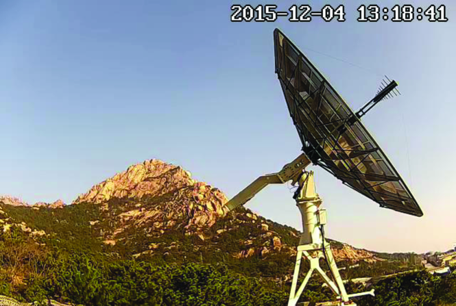
Figure 1.: The CSO 6-meter parabolic dish and the dual-polarized log-periodic antenna feed.f1

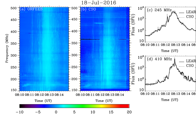
Figure 2.: (a, b) The solar radio dynamic spectra recorded by ORFEES and CSO at 150 – 500 MHz. (c, d) Solar radio burst flux density profiles observed at 245 MHz and 410 MHz by the LEAR and CSO. See text for details. The color bar indicates the relative intensity (the same below). f1

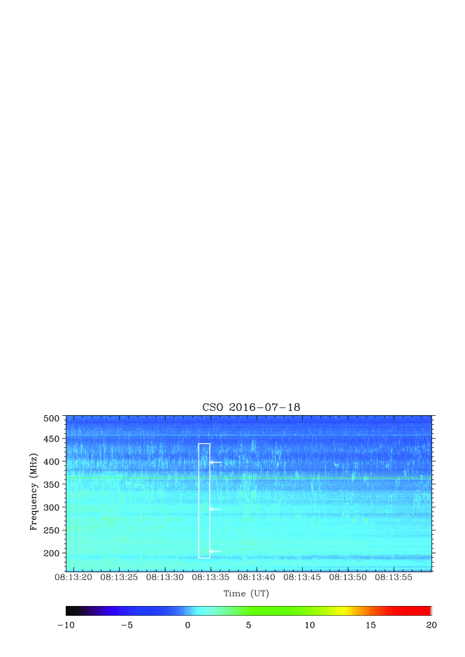
Figure 3.: The solar radio spikes observed by the CSO spectrograph at metric wavelengths. The temporal resolution of the data is 10 ms. The white rectangular box indicates three rows of solar radio spike clusters with similar structures at 200 MHz, 300 MHz, and 400 MHz, as pointed out by white arrows.f2

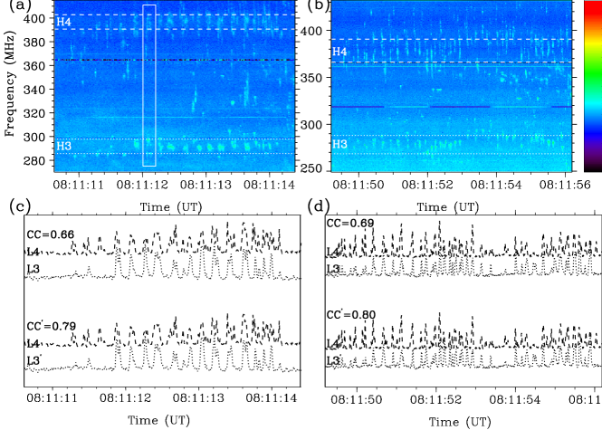
Figure 4.: (a, b) Spectra of two sets of solar radio spike clusters with the third and fourth harmonics. The dotted (H3) and dashed line pairs (H4) are used to indicate two spike clusters with similar morphology. (c) Dotted (L3) and dashed profiles (L4) are the light curves of integration and normalization of the radio spike burst intensity between the two line pairs (H3 and H4), and L3^′ is the light curve of L3 shifted forward by 10 ms. (d) Profiles are the same as those of (c) but obtained from the spectrum of (b).f3

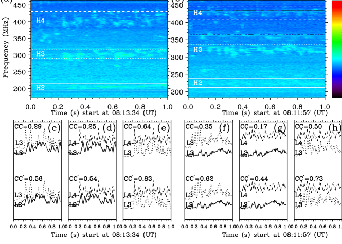
Figure 5.: (a, b) Spectra of two sets of solar radio spike clusters with the second, third, and fourth harmonics. The solid (H2), dotted (H3), and dashed line pairs (H4) are used to indicate three spike clusters with similar morphology. (c – e) solid (L2), dotted (L3), and dashed profiles (L4) are the light curves of integration and normalization of the radio spike burst intensity between the two line pairs (H2, H3, and H4), and L2^′, L2^′′, and L3^′ are the light curves of L2, L2, and L3 shifted forward by 30 ms, 40 ms, and 10 ms. (f – h) Profiles are the same as those of (c – e) but obtained from the spectrum of (b), and L2^′, L2^′′, and L3^′ are the light curves of L2, L2, and L3 shifted forward by 20 ms, 30 ms, and 10 ms.f4

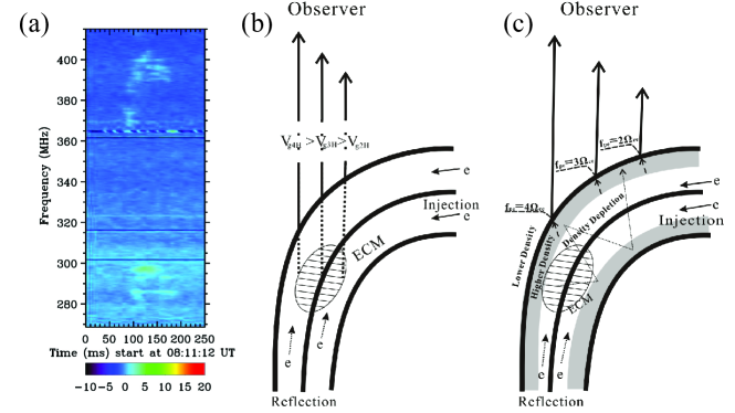
Figure 6.: (a) The radio spectrum of the inverted V-shape radio spike clusters. (b, c) The schematics for the causes of temporal delay of lower harmonics relative to higher orders and the formation of inverted V-shape clusters. The energetic electrons accelerated from magnetic field reconnection are injected into the magnetic loop system, and because of the magnetic mirror effect the electrons are reflected above the magnetic loop foot point. Electrons with different distributions are unstable and can efficiently drive ECM. The injected and reflected electrons result in the emission of the first and second branches of the inverted V-shape spike cluster, respectively. (b) The group velocities of the second, third, and fourth harmonics are different (V_g4H $>$ V_g3H $>$ V_g2H) and this difference can cause the time delay. (c) When the ECM emission propagates in a centeral density depleted magnetic loop (the surface density is higher and the surrounding density is lower), the fourth harmonic escapes at the lower site with the plasma frequency $f_{\mathrm{pe}}$=4 $\Omega_{\mathrm{ce}}$, and the third and second harmonics escape at relatively higher sites of the magnetic loop structures with the plasma frequencies being 3 $\Omega_{\mathrm{ce}}$ and 2 $\Omega_{\mathrm{ce}}$. So, the lower harmonics take a longer time to escape from the magnetic loop. f5

References

- Benz (1986) Benz, A.O.: 1986, Millisecond radio spikes. Sol. Phys. 104, 99. DOI. ADS.
- Benz and Guedel (1987) Benz, A.O., Guedel, M.: 1987, Harmonic emission and polarization of millisecond radio spikes. Sol. Phys. 111, 175. DOI. ADS.
- Bingham et al. (2013) Bingham, R., Speirs, D.C., Kellett, B.J., Vorgul, I., McConville, S.L., Cairns, R.A., Cross, A.W., Phelps, A.D.R., Ronald, K.: 2013, Laboratory astrophysics: Investigation of planetary and astrophysical maser emission. Space Sci. Rev. 178, 695. DOI. ADS.
- Bouratzis et al. (2015) Bouratzis, C., Hillaris, A., Alissandrakis, C.E., Preka-Papadema, P., Moussas, X., Caroubalos, C., Tsitsipis, P., Kontogeorgos, A.: 2015, Fine Structure of Metric Type IV Radio Bursts Observed with the ARTEMIS-IV Radio-Spectrograph: Association with Flares and Coronal Mass Ejections. Sol. Phys. 290, 219. DOI. ADS.
- Bouratzis et al. (2016) Bouratzis, C., Hillaris, A., Alissandrakis, C.E., Preka-Papadema, P., Moussas, X., Caroubalos, C., Tsitsipis, P., Kontogeorgos, A.: 2016, High resolution observations with Artemis-IV and the NRH. I. Type IV associated narrow-band bursts. A&A 586, A29. DOI. ADS.
- Chernov (2011) Chernov, G.P. (ed.): 2011, Fine Structure of Solar Radio Bursts, Astrophysics and Space Science Library 375. DOI. ADS.
- Cliver, White, and Balasubramaniam (2011) Cliver, E.W., White, S.M., Balasubramaniam, K.S.: 2011, The Solar Decimetric Spike Burst of 2006 December 6: Possible Evidence for Field-aligned Potential Drops in Post-eruption Loops. ApJ 743, 145. DOI. ADS.
- Dorovskyy et al. (2015) Dorovskyy, V.V., Melnik, V.N., Konovalenko, A.A., Bubnov, I.N., Gridin, A.A., Shevchuk, N.V., Rucker, H.O., Poedts, S., Panchenko, M.: 2015, Decameter U-burst Harmonic Pair from a High Loop. Sol. Phys. 290, 181. DOI. ADS.
- Dory, Guest, and Harris (1965) Dory, R.A., Guest, G.E., Harris, E.G.: 1965, Unstable Electrostatic Plasma Waves Propagating Perpendicular to a Magnetic Field. Physical Review Letters 14, 131. DOI. ADS.
- Du et al. (2017) Du, Q.-F., Chen, L., Zhao, Y.-C., Li, X., Zhou, Y., Zhang, J.-R., Yan, F.-B., Feng, S.-W., Li, C.-Y., Chen, Y.: 2017, A solar radio dynamic spectrograph with flexible temporal-spectral resolution. Research in Astronomy and Astrophysics 17, 098. DOI. ADS.
- Ergun et al. (2000) Ergun, R.E., Carlson, C.W., McFadden, J.P., Delory, G.T., Strangeway, R.J., Pritchett, P.L.: 2000, Electron-Cyclotron Maser Driven by Charged-Particle Acceleration from Magnetic Field-aligned Electric Fields. ApJ 538, 456. DOI. ADS.
- Fleishman and Mel’nikov (1998) Fleishman, G.D., Mel’nikov, V.F.: 1998, REVIEWS OF TOPICAL PROBLEMS: Millisecond solar radio spikes. Physics Uspekhi 41, 1157. DOI. ADS.
- Guedel (1990) Guedel, M.: 1990, Solar radio spikes - Radiation at harmonics S = 2-6. A&A 239, L1. ADS.
- Kong et al. (2016) Kong, X., Chen, Y., Feng, S., Du, G., Li, C., Koval, A., Vasanth, V., Wang, B., Guo, F., Li, G.: 2016, Observation of a Metric Type N Solar Radio Burst. ApJ 830, 37. DOI. ADS.
- Krucker and Benz (1994) Krucker, S., Benz, A.O.: 1994, The frequency ratio of bands of microwave spikes during solar flares. A&A 285, 1038. ADS.
- Leblanc, Dulk, and Bougeret (1998) Leblanc, Y., Dulk, G.A., Bougeret, J.-L.: 1998, Tracing the Electron Density from the Corona to 1au. Sol. Phys. 183, 165. DOI. ADS.
- Melnik et al. (2014) Melnik, V.N., Shevchuk, N.V., Konovalenko, A.A., Rucker, H.O., Dorovskyy, V.V., Poedts, S., Lecacheux, A.: 2014, Solar Decameter Spikes. Sol. Phys. 289, 1701. DOI. ADS.
- Messmer, Benz, and Monstein (1999) Messmer, P., Benz, A.O., Monstein, C.: 1999, PHOENIX-2: A New Broadband Spectrometer for Deci- metric and Microwave Radio Bursts First Results. Sol. Phys. 187, 335. DOI. ADS.
- Morosan et al. (2016) Morosan, D.E., Zucca, P., Bloomfield, D.S., Gallagher, P.T.: 2016, Conditions for electron-cyclotron maser emission in the solar corona. A&A 589, L8. DOI. ADS.
- Newkirk (1961) Newkirk, G. Jr.: 1961, The Solar Corona in Active Regions and the Thermal Origin of the Slowly Varying Component of Solar Radio Radiation. ApJ 133, 983. DOI. ADS.
- Shevchuk et al. (2016) Shevchuk, N.V., Melnik, V.N., Poedts, S., Dorovskyy, V.V., Magdalenic, J., Konovalenko, A.A., Brazhenko, A.I., Briand, C., Frantsuzenko, A.V., Rucker, H.O., Zarka, P.: 2016, The Storm of Decameter Spikes During the Event of 14 June 2012. Sol. Phys. 291, 211. DOI. ADS.
- Trievelpiece, Pechacek, and Kapetanakos (1968) Trievelpiece, A.W., Pechacek, R.E., Kapetanakos, C.A.: 1968, Trapping of a 0.5-MeV Electron Ring in a 15-kG Pulsed Magnetic Mirror Field. Physical Review Letters 21, 1436. DOI. ADS.
- Wu (1985) Wu, C.S.: 1985, Kinetic cyclotron and synchrotron maser instabilities - Radio emission processes by direct amplification of radiation. Space Sci. Rev. 41, 215. DOI. ADS.
- Wu and Lee (1979) Wu, C.S., Lee, L.C.: 1979, A theory of the terrestrial kilometric radiation. ApJ 230, 621. DOI. ADS.
- Wu et al. (2002) Wu, C.S., Wang, C.B., Yoon, P.H., Zheng, H.N., Wang, S.: 2002, Generation of Type III Solar Radio Bursts in the Low Corona by Direct Amplification. ApJ 575, 1094. DOI. ADS.
- Wu et al. (2005) Wu, C.S., Wang, C.B., Zhou, G.C., Wang, S., Yoon, P.H.: 2005, Altitude-dependent Emission of Type III Solar Radio Bursts. ApJ 621, 1129. DOI. ADS.
- Xie et al. (2017) Xie, H., Madjarska, M.S., Li, B., Huang, Z., Xia, L., Wiegelmann, T., Fu, H., Mou, C.: 2017, The Plasma Parameters and Geometry of Cool and Warm Active Region Loops. ApJ 842, 38. DOI. ADS.
- Zhao et al. (2016a) Zhao, G.Q., Feng, H.Q., Wu, D.J., Chen, L., Tang, J.F., Liu, Q.: 2016a, Cyclotron Maser Emission from Power-law Electrons with Strong Pitch-angle Anisotropy. ApJ 822, 58. DOI. ADS.
- Zhao et al. (2016b) Zhao, G.Q., Chu, Y.H., Feng, H.Q., Wu, D.J.: 2016b, The effect of electron holes on cyclotron maser emission driven by horseshoe distributions. Physics of Plasmas 23(11), 114505. DOI. ADS.