Hierarchy of the nonlocal advantage of quantum coherence and Bell nonlocality

Abstract

Quantum coherence and nonlocality capture nature of quantumness from different aspects. For the two-qubit states with diagonal correlation matrix, we prove strictly a hierarchy between the nonlocal advantage of quantum coherence (NAQC) and Bell nonlocality by showing geometrically that the NAQC created on one qubit by local measurement on another qubit captures quantum correlation which is stronger than Bell nonlocality. For general states, our numerical results present strong evidence that this hierarchy may still hold. So the NAQC states form a subset of the states that can exhibit Bell nonlocality. We further propose a measure of NAQC that can be used for a quantitative study of it in bipartite states.

I Introduction

Quantum correlations in states of composite systems can be characterized from different perspectives. From the applicative point of view, they are also invaluable physical resources which are recognized to be responsible for the power of those classically impossible tasks involving quantum communication and quantum computation Nielsen . Stimulated by this realization, there are a number of quantum correlation measures being put forward up to date nonlocal ; entangle ; steer ; discord . Some of the extensively studied measures include Bell nonlocality (BN) nonlocal , quantum entanglement entangle , Einstein-Podolski-Rosen steering steer , and quantum discord discord . For two-qubit states, a hierarchy of these quantum correlations has also been identified new01 ; new02 ; hierarchy ; Angelo1 ; Angelo2 ; Angelo3 . This hierarchy reveals different yet interlinked subtle nature of correlations, and broadens our understanding about the physical essence of quantumness in a state.

Quantum coherence is another basic notion in quantum theory, and recent years have witnessed an increasing interest on pursuing its quantification Plenio ; Hu . In particular, based on a seminal framework formulated by Baumgratz et al. coher , there are various coherence measures being proposed meas6 ; asym1 ; co-ski2 ; meas4 ; dist2 ; measjpa ; new1 . This stimulates one’s enthusiasm to understand them from different aspects, as for instance the distillation of coherence dist2 ; distill , the role of coherence played in quantum state merging qsm , and the characteristics of coherence under local quantum operations create1 ; create2 ; mc1 ; mc2 and noisy quantum channels fro1 ; fro2 . Moreover, some fundamental aspects of coherence such as its role in revealing the wave nature of a system path1 ; path2 , its tradeoffs under the mutually unbiased bases comple1 or incompatible bases comple2 , have also been extensively studied.

Conceptually, coherence is thought to be more fundamental than various forms of quantum correlations, hence it is natural to pursue their interrelations for bipartite and multipartite systems. In fact, it has already been shown that coherence itself can be quantified by the entanglement created between the considered system and an incoherent ancilla meas1 . There are also several works which linked coherence to quantum discord Yao ; Ma ; Hufan and measurement-induced disturbance Huxy .

In a recent work, Mondal et al. naqc explored the interrelation of quantum coherence and quantum correlations from an operational perspective. By performing local measurements on qubit $A$ of a two-qubit state $AB$, they showed that the average coherence of the conditional states of $B$ summing over the mutually unbiased bases can exceed a threshold that cannot be exceeded by any single-qubit state. They termed this as the nonlocal advantage of quantum coherence (NAQC), and proved that any two-qubit state that can achieve a NAQC (we will call it the NAQC state for short) is quantum entangled. As there are many other quantum correlation measures, it is significant to purse their connections with NAQC. We explore such a problem in this paper. For two-qubit states with diagonal correlation matrix, we showed strictly that quantum correlation responsible for NAQC is stronger than that responsible for BN, while for general states this result is conjectured based on numerical analysis. We hope this finding may shed some light on our current quest for a deep understanding of the interrelation between quantum coherence and quantum correlations in composite systems.

II Technical preliminaries

We start by recalling two well-established coherence measures known as the $l_{1}$ norm of coherence and relative entropy of coherence coher . For a state described by density operator $\rho$ in the reference basis $\{|i\rangle\}$, they are given, respectively, by

$$C_{l_{1}}(\rho)=\sum_{i\neq j}|\langle i|\rho|j\rangle|,\;C_{re}(\rho)=S(\rho_{\mathrm{diag}})-S(\rho),$$ (1)

where $S(\cdot)$ denotes the von Neumann entropy, and $\rho_{\mathrm{diag}}$ is an operator comprised of the diagonal part of $\rho$.

Using the above measures, Mondal et al. presented a “steering game” in Ref. naqc : Two players, Alice and Bob, share a two-qubit state $\rho$. They begin this game by agreeing on three observables $\{\sigma_{1},\sigma_{2},\sigma_{3}\}$, with $\sigma_{1,2,3}$ being the usual Pauli operators. Alice then measures qubit A and informs Bob of her choice $\sigma_{i}$ and outcome $a\in\{0,1\}$. Finally, Bob measures coherence of qubit B in the eigenbasis of either $\sigma_{j}$ or $\sigma_{k}$ ($j,k\neq i$) randomly. By denoting the ensemble of his conditional states as $\{p(a|\sigma_{i}),\rho_{B|\sigma_{i}^{a}}\}$, the average coherence is given by

$$\bar{C}_{\alpha}^{\sigma_{j}}(\{p(a|\sigma_{i}),\rho_{B|\sigma_{i}^{a}}\})=\sum_{a}p(a|\sigma_{i})C_{\alpha}^{\sigma_{j}}(\rho_{B|\sigma_{i}^{a}}),$$ (2)

where $p(a|\sigma_{i})=\mathrm{tr}(\Pi_{i}^{a}\rho)$, $\rho_{B|\sigma_{i}^{a}}=\mathrm{tr}_{A}(\Pi_{i}^{a}\rho)/p(a|\sigma_{i})$, $\Pi_{i}^{a}=[I_{2}+(-1)^{a}\sigma_{i}]/2$, $I_{2}$ is the identity operator, and $C_{\alpha}^{\sigma_{j}}$ ($\alpha=l_{1}$ or $re$) is the coherence defined in the eigenbasis of $\sigma_{j}$.

By further averaging over the three possible measurements of Alice and the corresponding possible reference eigenbases chosen by Bob, Mondal et al. naqc derived the criterion for achieving NAQC, which is given by

$$C_{\alpha}^{na}(\rho)=\frac{1}{2}\sum_{i,j,a\atop i\neq j}p(a|\sigma_{i})C^{\sigma_{j}}_{\alpha}(\rho_{B|\sigma_{i}^{a}})>C_{\alpha}^{m},$$ (3)

where $C_{l_{1}}^{m}=\sqrt{6}$, $C_{re}^{m}=3H(1/2+\sqrt{3}/6)\simeq 2.2320$, and $H(\cdot)$ stands for the binary Shannon entropy function.

In fact, the above critical values are also direct results of the complementarity relations of coherence under mutually unbiased bases comple1 . To be explicit, by Eq. (4) of Ref. comple1 and the mean inequality (the arithmetic mean of a list of nonnegative real numbers is not larger than the quadratic mean of the same list) one can obtain the critical value $C_{l_{1}}^{m}$, while from Eq. (24) of Ref. comple1 one can obtain the critical value $C_{re}^{m}$.

To detect nonlocality in $\rho$, one can use the Bell-CHSH inequality $|\langle B_{\mathrm{CHSH}}\rangle_{\rho}|\leqslant 2$, where $B_{\mathrm{CHSH}}$ is the Bell operator chsh . Violation of this inequality implies that $\rho$ is Bell nonlocal. The maximum of $|B_{\mathrm{CHSH}}\rangle_{\rho}|$ over all mutually orthogonal pairs of unit vectors in $\mathbb{R}^{3}$ is given by chsh2

$$B_{\max}(\rho)=2\sqrt{M(\rho)},$$ (4)

where $M(\rho)=u_{1}+u_{2}$, with $u_{i}$ ($i=1,2,3$) being the eigenvalues of $T^{\dagger}T$ arranged in nonincreasing order, and $T$ stands for the matrix formed by elements $t_{ij}=\mathrm{tr}(\rho\sigma_{i}\otimes\sigma_{j})$. Clearly, $M(\rho)>1$ is also a manifestation of BN in $\rho$.

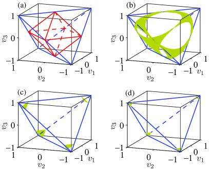
Figure 1: The tetrahedron $\mathcal{T}$ and octahedron $\mathcal{O}$ associated with $\rho_{\mathrm{Bell}}$ (a), and the level surfaces of $M(\tilde{\rho})=1$ (b), $C_{l_{1}}^{na}(\rho_{\mathrm{Bell}})=\sqrt{6}$ (c), and $C_{re}^{na}(\rho_{\mathrm{Bell}})=C_{re}^{m}$ (d). The regions of Bell nonlocal states $\tilde{\rho}$ and NAQC states $\rho_{\mathrm{Bell}}$ are those outside the level surfaces.

It has been shown that any $\rho$ that can achieve a NAQC is entangled, while the opposite case is not always true naqc . This gives rise to a hierarchy of them. To further establish the hierarchy between NAQC and BN, and based on the consideration that the BN is local unitary invariant, we first consider the representative class of two-qubit states

$$\tilde{\rho}=\frac{1}{4}\Bigl{(}I_{4}+\vec{r}\cdot\vec{\sigma}\otimes I_{2}+I_{2}\otimes\vec{s}\cdot\vec{\sigma}+\sum_{i=1}^{3}v_{i}\sigma_{i}\otimes\sigma_{i}\Bigr{)},$$ (5)

where $\{\vec{r},\vec{s},\vec{v}\}\in\mathbb{R}^{3}$ satisfy the physical requirement $\tilde{\rho}\geqslant 0$. For $\vec{r}=\vec{s}=0$, it reduces to the Bell-diagonal state $\rho_{\mathrm{Bell}}$ which is characterized by the tetrahedron $\mathcal{T}$ [see Fig. 1(a)], and the region of separable $\rho_{\mathrm{Bell}}$ is the octahedron $\mathcal{O}$ Horodecki . For $\vec{r}\cdot\vec{s}\neq 0$, physical $\tilde{\rho}$ shrinks to partial regions of $\mathcal{T}$. For this case, while the separable region is still inside $\mathcal{O}$, the entangled ones may not be limited to the four regions outside $\mathcal{O}$.

III Hierarchy of NAQC and BN

The hierarchy of entanglement, steering, and BN shows that while entanglement clearly reveals the nonclassical nature of a state, steering and BN exhibit even stronger deviations from classicality new01 ; new02 ; hierarchy ; Angelo1 ; Angelo2 ; Angelo3 . Here, we show that NAQC may be viewed as a quantum correlation which is even stronger than BN.

To begin with, we prove the convexity of NAQC,

$$C^{na}_{\alpha}\bigg{(}{\sum_{k}q_{k}\rho_{k}}\bigg{)}\leqslant\sum_{k}q_{k}C^{na}_{\alpha}(\rho_{k}),$$ (6)

that is, the NAQC is nonincreasing under mixing of states. By combining Eqs. (2) and (3), one can see that the NAQC is convex provided $\bar{C}^{\sigma_{j}}_{\alpha}$ is convex. For $\rho=\sum_{k}q_{k}\rho_{k}$, the conditional state of $B$ after Alice’s local measurements is

$$\rho_{B|\sigma_{i}^{a}}=\frac{\sum_{k}q_{k}\mathrm{tr}_{A}(\Pi_{i}^{a}\rho_{k})}{\sum_{k}q_{k}\mathrm{tr}(\Pi_{i}^{a}\rho_{k})}=\frac{\sum_{k}q_{k}p_{k}(a|\sigma_{i})\rho_{B|\sigma_{i}^{a}}^{k}}{p(a|\sigma_{i})},$$ (7)

where $\rho_{B|\sigma_{i}^{a}}^{k}=\mathrm{tr}_{A}(\Pi_{i}^{a}\rho_{k})/p_{k}(a|\sigma_{i})$, $p_{k}(a|\sigma_{i})=\mathrm{tr}(\Pi_{i}^{a}\rho_{k})$, and we have denoted by $p(a|\sigma_{i})=\sum_{k}q_{k}p_{k}(a|\sigma_{i})$. Then

$$\bar{C}^{\sigma_{j}}_{\alpha}\big{(}\{p(a|\sigma_{i}),\rho_{B|\sigma_{i}^{a}}\}\big{)} =\sum_{a}p(a|\sigma_{i})C^{\sigma_{j}}_{\alpha}(\rho_{B|\sigma_{i}^{a}})$$ (8)

$$\leqslant\sum_{k,a}p(a|\sigma_{i})\frac{q_{k}p_{k}(a|\sigma_{i})}{p(a|\sigma_{i})}C^{\sigma_{j}}_{\alpha}\bigl{(}\rho_{B|\sigma_{i}^{a}}^{k}\bigr{)}$$

$$=\sum_{k,a}q_{k}p_{k}(a|\sigma_{i})C^{\sigma_{j}}_{\alpha}\bigl{(}\rho_{B|\sigma_{i}^{a}}^{k}\bigr{)}$$

$$=\sum_{k}q_{k}\bar{C}^{\sigma_{j}}_{\alpha}\big{(}\{p_{k}(a|\sigma_{i}),\rho_{B|\sigma_{i}^{a}}^{k}\}\big{)},$$

where the first inequality is due to convexity of the coherence measure. This completes the proof of Eq. (6).

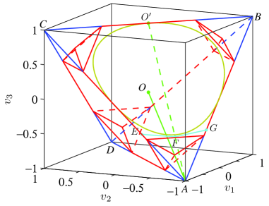
Figure 2: Geometric representation of the polyhedron $\mathcal{P}$ (the red lines) inside $\mathcal{T}$. Here, $O$ and $O^{\prime}$ are the coordinate origin and the midpoint of $BC$, respectively, while the khaki curve is the curve of constant BN $M(\tilde{\rho})=1$ at the facet $ABC$.

Next, we give the level surface $\mathcal{S}$ of constant BN $M(\tilde{\rho})=1$. It can be divided into four parts, corresponding to the four vertices of $\mathcal{T}$. For convenience of later presentation, we denote by $\mathcal{S}_{A}$ the part near vertex $A$ (see Fig. 2). It is described by

$$v_{i}=\sin\theta,~{}v_{j}=\cos\theta,$$ (9)

$$v_{k}\in[\max\{\sin\theta,\cos\theta\},1+\sin\theta+\cos\theta],~{}\theta\in[\pi,1.5\pi],$$

where $(i,j,k)=(1,2,3)$, $(2,3,1)$, and $(3,1,2)$. The equations for the other three parts of $\mathcal{S}$ can be obtained directly by their symmetry about the coordinate origin $O$. The corresponding results are showed in Fig. 1(b).

In the following, we denote by $\mathcal{N}$ the set of NAQC states and $\mathcal{B}$ the set of Bell nonlocal states. We will prove the inclusion relation $\mathcal{N}\subset\mathcal{B}$ for any $\tilde{\rho}$, meaning that the existence of NAQC implies the existence of BN.

III.1 $l_{1}$ norm of of NAQC

First, we consider the class of Bell-diagonal states. Without loss of generality, we assume $|v_{1}|\geqslant|v_{2}|\geqslant|v_{3}|$, then

$$C_{l_{1}}^{na}(\rho_{\mathrm{Bell}})=\sum_{i}|v_{i}|,~{}M(\rho_{\mathrm{Bell}})=v_{1}^{2}+v_{2}^{2},$$ (10)

from which one can obtain $|v_{1}|>\sqrt{6}/3$ and $|v_{2}|>(\sqrt{6}-1)/2$ when $C_{l_{1}}^{na}(\rho_{\mathrm{Bell}})>\sqrt{6}$. This further gives rise to $M(\rho_{\mathrm{Bell}})>1$. That is, any $\rho_{\mathrm{Bell}}$ that can achieve a NAQC is Bell nonlocal. But the converse is not true, e.g., if $v_{1,2,3}\in[-\sqrt{6}/3,-1/\sqrt{2})$, we have $M(\rho_{\mathrm{Bell}})>1$ and $C_{l_{1}}^{na}(\rho_{\mathrm{Bell}})\leqslant\sqrt{6}$. With all this, we arrived at the inclusion relation $\mathcal{N}\subset\mathcal{B}$. The level surfaces of $C_{l_{1}}^{na}(\rho_{\mathrm{Bell}})=\sqrt{6}$ can be found in Fig. 1(c).

Second, we consider $\tilde{\rho}$ sitting at the edges of $\mathcal{T}$ with general $\vec{r}$ and $\vec{s}$. We take the edge $AB$ as an example (see Fig. 2), the cases for the other edges are similar. Along this edge, we have $v_{1}=v_{3}$ and $v_{2}=-1$, then one can determine analytically the constraints imposed by $\tilde{\rho}\geqslant 0$ on the involved parameters as $r_{1,3}=s_{1,3}=0$, $r_{2}=-s_{2}$, and $s_{2}^{2}\leqslant 1-v_{1}^{2}$ (see Appendix A). Thus we have

$$C_{l_{1}}^{na}(\tilde{\rho})=1+|v_{1}|+\sqrt{v_{1}^{2}+s_{2}^{2}}.$$ (11)

It is always not larger than $\sqrt{6}$ in the region of $|v_{1}|\leqslant\sqrt{6}-2$. On the other hand, the states located at the edge $AB$ other than its midpoint are Bell nonlocal. Hence, the inclusion relation $\mathcal{N}\subset\mathcal{B}$ holds for all $\tilde{\rho}$ located at the edges of $\mathcal{T}$.

Next, we consider $\tilde{\rho}$ associated with $v_{1,2,3}=v_{0}=-1/\sqrt{2}$. As $C_{l_{1}}^{na}$ is an increasing function of $|s_{i}|$ ($i=1,2,3$), one only needs to determine the maximal $|s_{i}|$ for which $\tilde{\rho}\geqslant 0$. Without loss of generality, we assume $s_{3}=w_{0}s_{1}$ and $s_{2}=w_{1}s_{1}$, then a detailed analysis shows that the resulting maximum NAQC states belong to the set of $\tilde{\rho}$ with $r_{3}=w_{0}r_{1}$ and $r_{2}=w_{1}r_{1}$. Under this condition, one can obtain analytically the eigenvalues $\epsilon_{k}$ of $\tilde{\rho}$. Then from $\epsilon_{k}\geqslant 0$ ($\forall k$) one can obtain

$$|s_{1}+r_{1}|\leqslant c_{1}=\frac{1+v_{0}}{\sqrt{1+w_{0}^{2}+w_{1}^{2}}},$$ (12)

$$|s_{1}-r_{1}|\leqslant c_{2}=\sqrt{\frac{1-2v_{0}-3v_{0}^{2}}{1+w_{0}^{2}+w_{1}^{2}}}.$$

For state $\tilde{\rho}$ with fixed $v_{0}$, $w_{0}$, and $w_{1}$, $C_{l_{1}}^{na}$ takes its maximum when the above inequalities become equalities. That is, when

$$s_{1}=\pm\frac{1}{2}(c_{1}+c_{2}),~{}r_{1}=\pm\frac{1}{2}(c_{1}-c_{2}),$$ (13)

then by further maximizing the resulting $C_{l_{1}}^{na}$ over $w_{0}$ and $w_{1}$, we obtain $C_{l_{1},\max}^{na}\simeq 2.4405$ at the critical points $w_{0,1}=\pm 1$ (we have also checked the validity of this result with $10^{7}$ randomly generated $\tilde{\rho}$ for which $v_{1,2,3}=-1/\sqrt{2}$, and no violation was observed). As this maximum is smaller than $\sqrt{6}$, any $\tilde{\rho}$ with $v_{0}=-1/\sqrt{2}$ cannot achieve a NAQC.

To proceed, we introduce a polyhedron $\mathcal{P}$ with the set of its vertices near the vertex $A$ being given by $(v_{0},v_{0},v_{0})$, $(-1,\gamma,\gamma)$, $(\gamma,-1,\gamma)$, $(\gamma,\gamma,-1)$, and its other vertices can be obtained by using their symmetry with respect to the point $O$ (see Fig. 2). One can show that when $|\gamma|<\sqrt{2}-1$, the surface $\mathcal{S}_{A}$ is always inside $\mathcal{P}$ (see Appendix B). Finally, as $C_{l_{1},\max}^{na}\simeq 2.4405$ at the point $(v_{0},v_{0},v_{0})$, we choose $\gamma=2-\sqrt{6}$ for which $C_{l_{1}}^{na}$ is also smaller than $\sqrt{6}$ at the other three points of $\mathcal{P}$ near vertex $A$ [see Eq.(11)], then as any physical state with $\vec{v}$ inside $\mathcal{P}$ can be written as a convex combination of states with $\vec{v}$ at the vertices of $\mathcal{P}$, we complete the proof of the inclusion relation $\mathcal{N}\subset\mathcal{B}$ for general $\tilde{\rho}$ by using the convexity of NAQC.

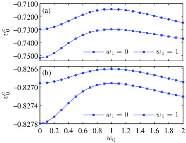
Figure 3: Critical $v_{0}^{c}$ for which (a) $C_{l_{1}}^{na}=\sqrt{6}$ and (b) $C_{re}^{na}=C_{re}^{m}$ versus $w_{0}$ with $w_{1}=0$ and 1. The other parameters are $\vec{s}=(s_{1},w_{0}s_{1},w_{1}s_{1})$ and $\vec{r}=(r_{1},w_{0}r_{1},w_{1}r_{1})$, with $s_{1}$ and $r_{1}$ being given in Eq. (13), and $v_{0}^{c}$ is plotted in the region of $v_{0}<0$.

In fact, for $\tilde{\rho}$ at the line $AO$ with fixed $w_{0}$ and $w_{1}$, one can obtain the critical $v_{0}^{c}$ at which $C_{l_{1}}^{na}=\sqrt{6}$. As $C_{l_{1}}^{na}$ and $v_{0}^{c}$ considered here are invariant under the substitution $w_{0}\leftrightarrow w_{1}$, we showed in Fig. 3(a) an exemplified plot of the $w_{0}$ dependence of $v_{0}^{c}$ with fixed $w_{1}=0$ and 1. It first increases to a peak value at $w_{0}=1$, then decreases gradually with the increase of $|\omega_{0}|$. By optimizing over $w_{0}$ and $w_{1}$, one can further obtain the region of $v_{0}^{c}\in(-0.7519,-0.7142)$, where the lower and upper bounds correspond to $w_{0,1}=0$ and $w_{0,1}=\pm 1$, respectively. Clearly, the point $(v_{0}^{c},v_{0}^{c},v_{0}^{c})$ is always outside the surface $\mathcal{S}$.

III.2 Relative entropy of NAQC

In this subsection, we consider NAQC measured by the relative entropy. First, for Bell-diagonal states, the corresponding NAQC can be obtained as naqc

$$C_{re}^{na}(\rho_{\mathrm{Bell}})=3-\sum_{i}H\Biggl{(}\frac{1+v_{i}}{2}\Biggr{)}.$$ (14)

Then by imposing $C_{re}^{na}(\rho_{\mathrm{Bell}})>C_{re}^{m}$ with the assumption $|v_{1}|\geqslant|v_{2}|\geqslant|v_{3}|$, one can obtain

$$H\Biggl{(}\frac{1+v_{1}}{2}\Biggr{)}<\frac{3-C_{re}^{m}}{3},~{}H\Biggl{(}\frac{1+v_{2}}{2}\Biggr{)}<\frac{3-C_{re}^{m}}{2},$$ (15)

which yields $M(\rho_{\mathrm{Bell}})>1$. Moreover, we have $M(\rho_{\mathrm{Bell}})>1$ and $C_{re}^{na}(\rho_{\mathrm{Bell}})<C_{re}^{m}$ for $v_{1,2,3}\in(-0.9140,-1/\sqrt{2})$. So $\mathcal{N}\subset\mathcal{B}$ holds for $\rho_{\mathrm{Bell}}$. The corresponding level surfaces were showed in Fig. 1(d). Clearly, the region of NAQC states shrinks compared with that captured by the $l_{1}$ norm.

For $\tilde{\rho}$ sitting at the edges of $\mathcal{T}$ with general $\vec{r}$ and $\vec{s}$, we take the edge $AB$ as an example. Based on the results of Sec. III.1, one can obtain

$$C_{re}^{na}=2+H\Biggl{(}\frac{1+s_{2}}{2}\Biggr{)}-2H\left(\frac{1+\sqrt{v_{1}^{2}+s_{2}^{2}}}{2}\right),$$ (16)

then it is direct to show that $C_{re}^{na}$ is always smaller than $C_{re}^{m}$ for $|v_{1}|<-b_{0}\simeq 0.3813$. So the inclusion relation $\mathcal{N}\subset\mathcal{B}$ holds for any $\tilde{\rho}$ at the edges of $\mathcal{T}$.

Based on the above preliminaries, we now consider $\tilde{\rho}$ at the surface $\mathcal{S}_{A}$ (the cases for the other parts of $\mathcal{S}$ are similar). We will show that for these $\tilde{\rho}$ the inequality $C_{re}^{na}<C_{re}^{m}$ holds. Then by further employing the convexity of NAQC and the fact that $\{\tilde{\rho}\}$ is a convex set, one can complete the proof of $\mathcal{N}\subset\mathcal{B}$. In fact, due to the structure of $\mathcal{S}_{A}$ [see Eq. (9)], it suffices to prove that we always have $C_{re}^{na}<C_{re}^{m}$ at the boundary of $\mathcal{S}_{A}$.

First, we introduce the polygon line $EFG$ over $(-1,b_{0},b_{0})$, $(a_{0},a_{0},1+2a_{0})$, and $(b_{0},-1,b_{0})$. One can prove that there is no intersection of this line and the boundary of $\mathcal{S}_{A}$ at the facet $ABC$ when $a_{0}\lesssim-0.7082$ (Appendix B). Moreover, along the line $AO^{\prime}$, $\tilde{\rho}\geqslant 0$ yields $r_{1,2}=-s_{1,2}$ and $r_{3}=s_{3}$ (Appendix A), then one can obtain that at the point $F$ with $a_{0}=-0.7082$, $C_{re}^{na}$ maximized over $\vec{r}$ and $\vec{s}$ is of about 1.4956. As $C_{re}^{na}$ is also smaller than $C_{re}^{m}$ at the points $E$ and $G$ [see Eq. (16)], we have $C_{re}^{na}<C_{re}^{m}$ for any $\tilde{\rho}$ at this boundary.

Second, if we make the substitutions $v_{0}=-0.7082$ and $\gamma=b_{0}$ to the vertices of $\mathcal{P}$, then one can show that the boundary of $\mathcal{S}_{A}$ inside $\mathcal{T}$ is also inside $\mathcal{P}$ (see Appendix B). For $\tilde{\rho}$ at the point $(v_{0},v_{0},v_{0})$, our numerical results showed that with fixed $v_{0}$, $w_{0}$, and $w_{1}$, $C_{re}^{na}$ also takes its maximum when $s_{1}$ and $r_{1}$ are given by Eq. (13). Then by further maximizing it over $w_{0}$ and $w_{1}$, we obtain $C_{re,\max}^{na}\simeq 2.0041$ at $w_{0,1}=\pm 1$. As $C_{re}^{na}$ is also smaller than $C_{re}^{m}$ for $\tilde{\rho}$ at the vertices of $\mathcal{P}$ with $\gamma=b_{0}$ [see Eq. (16)], we have $C_{re}^{na}<C_{re}^{m}$ for any $\tilde{\rho}$ at this boundary.

Similar to the $l_{1}$ norm of NAQC, one can obtain $v_{0}^{c}$ at which $C_{re}^{na}=C_{re}^{m}$ with fixed $w_{0}$ and $w_{1}$. It is $v_{0}^{c}\in(-0.8278,-0.8266)$, where the lower and upper bounds are obtained with $w_{0,1}=0$ and $w_{0,1}=\pm 1$, respectively. As is showed in Fig. 3, $v_{0}^{c}$ for the two NAQCs exhibits qualitatively the same $w_{0}$ dependence.

Before ending this section, we would like to mention here that although for the set of Bell-diagonal states, one detects a wider region of NAQC states by using the $l_{1}$ norm as a measure of coherence than that by using the relative entropy (see Fig. 1), this is not always the case. A typical example is that for $\tilde{\rho}$ at the edge $AB$ of $\mathcal{T}$ with $|v_{1,3}|\in(0.3813,\sqrt{6}-2)$, one may have $C_{l_{1}}^{na}<\sqrt{6}$ and $C_{re}^{na}>C_{re}^{m}$.

IV An explicit application of NAQC

As it is a proven fact that all Bell nonlocal states are useful for quantum teleportation telep , the hierarchy we obtained implies that any NAQC state $\tilde{\rho}$ can serve as a quantum channel for quantum teleportation. That is, it always gives rise to the average fidelity $F_{av}>2/3$. In fact, $F_{av}$ achievable with the channel state $\tilde{\rho}$ is given by telep

$$F_{av}(\tilde{\rho})=\frac{1}{2}+\frac{1}{6}\sum_{i}|v_{i}|.$$ (17)

Using this equation and the results of Sec. III, one can obtain that for any NAQC state $\tilde{\rho}$ captured by $C_{l_{1}}^{na}(\tilde{\rho})$, we always have $F_{av}>\sqrt{6}/3$, while for any NAQC state $\tilde{\rho}$ captured by $C_{re}^{na}(\tilde{\rho})$, we always have $F_{av}\gtrsim 0.7938$. Both the two critical values are larger than $2/3$, so any NAQC state $\tilde{\rho}$ can serve as a quantum channel for nonclassical teleportation.

If we focus only on the class of NAQC Bell-diagonal states, the average fidelity $F_{av}$ can be further improved. More specifically, Eqs. (10) and (14) imply that $F_{av}>(3+\sqrt{6})/6$ for any NAQC state $\rho_{\mathrm{Bell}}$ captured by $C_{l_{1}}^{na}(\rho_{\mathrm{Bell}})$, and $F_{av}\gtrsim 0.9501$ for any NAQC state $\rho_{\mathrm{Bell}}$ captured by $C_{re}^{na}(\rho_{\mathrm{Bell}})$.

V Summary and discussion

In summary, we have explored the interrelations of NAQC achievable in a two-qubit state under local measurements and BN detected by violation of the Bell-CHSH inequality. There are two different scenarios of NAQC being considered: one is characterized by the $l_{1}$ norm of coherence, and another one is characterized by the relative entropy of coherence. For both scenarios, we showed geometrically that the inclusion relation $\mathcal{N}\subset\mathcal{B}$ holds for the class of states $\tilde{\rho}$ that have diagonal correlation matrix $T$. This extends the known hierarchy in quantum correlation, viz., BN, steerability, entanglement, and quantum discord to include NAQC.

One may also concern whether the obtained hierarchy holds for $\rho$ with nondiagonal $T$. As such $\rho$ is locally unitary equivalent to $\tilde{\rho}$, that is, $\rho=U_{AB}\tilde{\rho}U_{AB}^{\dagger}$ with $U_{AB}=U_{A}\otimes U_{B}$, the proof can be completed by showing that for any $\tilde{\rho}$ with $M(\tilde{\rho})\leqslant 1$, we have $C_{\alpha}^{na}(U_{AB}\tilde{\rho}U_{AB}^{\dagger})\leqslant C_{\alpha}^{m}$ for all unitaries $U_{AB}$. But due to the so many number of state parameters involved, it is difficult to give such a strict proof. For special cases, a strict proof may be available, e.g., for the locally unitary equivalent class of $\tilde{\rho}$ with $|\vec{v}|^{2}+2|\vec{s}|^{2}\leqslant 2$, we are sure that $C_{l_{1}}^{na}\leqslant\sqrt{6}$, while for the locally unitary equivalent class of $\rho_{\mathrm{Bell}}$, we are sure that $C_{re}^{na}\leqslant C_{re}^{m}$ (see Appendix C). Moreover, for $\tilde{\rho}$ with reduced number of parameters, we performed numerical calculations with $10^{7}$ equally distributed local unitaries generated according to the Haar measure Haar1 ; Haar2 , and found that $C_{\alpha}^{na}$ is always smaller than $C_{\alpha}^{m}$ (see Appendix C). These results presented strong evidence that the hierarchy may hold for any two-qubit state, though a strict proof is still needed.

Moreover, one may argue that NAQC can be recognized as a quantum correlation. It is stronger than BN in the sense that the NAQC states form a subset of the Bell nonlocal states. But it is asymmetric, that is, in general $C^{na}_{\alpha}$ defined with the local measurements on $A$ does not equal that defined with the local measurements on $B$. This property is the same to steerability and quantum discord. The NAQC is also not locally unitary invariant. Its value may be changed by performing local unitary transformation to the mutually unbiased bases. To avoid this perplexity, one can define

$$\tilde{C}_{\alpha}^{na}(\rho)=\frac{1}{2}\max_{\{U_{A}\otimes U_{B}\}}\sum_{i,j,a\atop i\neq j}p(a|\sigma_{i,U_{A}})C^{\sigma_{j,U_{B}}}_{\alpha}(\rho_{B|\sigma_{i,U_{A}}^{a}}),$$ (18)

with $\sigma_{i,U_{A}}=U_{A}\sigma_{i}U_{A}^{\dagger}$, and likewise for $\sigma_{j,U_{B}}$. As BN is locally unitary invariant, we have $\tilde{\mathcal{N}}\subset\mathcal{B}$ provided $\mathcal{N}\subset\mathcal{B}$, where $\tilde{\mathcal{N}}$ is the set of NAQC states captured by $\tilde{C}_{\alpha}^{na}(\rho)>C_{\alpha}^{m}$ .

Finally, in light of those measures of steerability based on the maximal violation of various steering inequalities and the similar measure of Bell nonlocality Angelo1 ; Angelo2 , it is natural to quantify the degree of NAQC in a bipartite state $\rho$ by

$$\tilde{Q}_{\alpha}(\rho)=\max\left\{0,\frac{\tilde{C}_{\alpha}^{na}(\rho)-C_{\alpha}^{m}}{\tilde{C}_{\alpha,\max}^{na}-C_{\alpha}^{m}}\right\},$$ (19)

where $\tilde{C}_{\alpha,\max}^{na}=\max_{\rho}\tilde{C}_{\alpha}^{na}(\rho)$, and the factor $\tilde{C}_{\alpha,\max}^{na}-C_{\alpha}^{m}$ was introduced for normalizing $\tilde{Q}_{\alpha}(\rho)$. For two-qubit states, we have $\tilde{C}_{\alpha,\max}^{na}=3$ ($\alpha=l_{1}$ or $re$), which are obtained for the Bell states $|\Phi^{\pm}\rangle=(|00\rangle\pm|11\rangle)/\sqrt{2}$ and $|\Psi^{\pm}\rangle=(|01\rangle\pm|10\rangle)/\sqrt{2}$. Moreover, we have used the fact that $C_{\alpha}^{m}$ cannot be increased by any unitary transformation in the above definition.

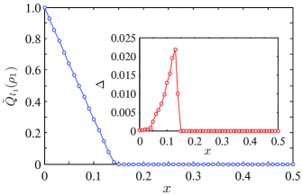
Figure 4: The $x$ dependence of $\tilde{Q}_{l_{1}}(\rho_{1})$. Here, we choose $x\in[0,0.5]$ as $\tilde{Q}_{l_{1}}(\rho_{1})$ is symmetric with respect to $x=0.5$ for $\rho_{1}$. The inset shows the $x$ dependence of $\Delta=\tilde{Q}_{l_{1}}(\rho_{1})-Q_{l_{1}}(\rho_{1})$.

Of course, one may propose to define the NAQC-based correlation measure [denoted $Q_{l_{1}}(\rho)$] by replacing $\tilde{C}_{\alpha}^{na}(\rho)$ in Eq. (19) with $C_{\alpha}^{na}(\rho)$. But if so, $Q_{l_{1}}(\rho)$ will not be locally unitary invariant, thus makes it violates the widely accepted property of a quantum correlation measure (e.g., Bell nonlocality, steerability, entanglement, and quantum discord) which should be locally unitary invariant.

As an example, we calculated numerically the NAQC-based correlation measure of the following state

$$\rho_{1}=x|\Phi^{+}\rangle\langle\Phi^{+}|+(1-x)|\Psi^{-}\rangle\langle\Psi^{-}|,~{}~{}x\in[0,1],$$ (20)

for which $\tilde{Q}_{l_{1}}(\rho_{1})$ is symmetric with respect to $x=0.5$. As was showed in Fig. 4, $\tilde{Q}_{l_{1}}(\rho_{1})>Q_{l_{1}}(\rho_{1})$ in the region of $0\lesssim x\lesssim 0.141$. In particular, we have $\tilde{Q}_{l_{1}}(\rho_{1})>0$ and $Q_{l_{1}}(\rho_{1})=0$ when $0.138\lesssim x\lesssim 0.141$, that is, $\tilde{Q}_{l_{1}}$ captures a wider region of NAQC states than $Q_{l_{1}}$.

Appendix A Constraints imposed on the parameters of $\tilde{\rho}$

At the edge $AB$ of $\mathcal{T}$, we have $v_{1}=v_{3}$ and $v_{2}=-1$. Then the positive semidefiniteness of $\tilde{\rho}$ requires

$$\tilde{\rho}_{11}\tilde{\rho}_{44}-|\tilde{\rho}_{14}|^{2}=-(r_{3}+s_{3})^{2}\geqslant 0,$$ (A1)

$$\tilde{\rho}_{22}\tilde{\rho}_{33}-|\tilde{\rho}_{23}|^{2}=-(r_{3}-s_{3})^{2}\geqslant 0,$$

from which one can obtain $r_{3}=s_{3}=0$.

Moreover, all the ith-order principal minors of $\tilde{\rho}$ should be nonnegative. Under the constraint $r_{3}=s_{3}=0$ obtained above, the second- and third-order leading principal minors $D_{2,3}$ and the principal minor $\Delta_{3}$ (determinant of the matrix obtained by removing from $\tilde{\rho}$ its third row and third column) are

$$D_{2}=1-v_{1}^{2}-s_{1}^{2}-s_{2}^{2},$$ (A2)

$$D_{3}=(v_{1}-1)[(r_{1}+s_{1})^{2}+(r_{2}+s_{2})^{2}],$$

$$\Delta_{3}=-(v_{1}+1)[(r_{1}-s_{1})^{2}+(r_{2}+s_{2})^{2}],$$

which, together with Eq. (A1), yields the following requirements

$$r_{1,3}=s_{1,3}=0,~{}r_{2}=-s_{2},~{}s_{2}^{2}\leqslant 1-v_{1}^{2}.$$ (A3)

Similarly, one can obtain constraints imposed on the parameters of $\tilde{\rho}$ at the other edges of $\mathcal{T}$. They are

$$AC\mathrm{:}~{}r_{2,3}=s_{2,3}=0,~{}r_{1}=-s_{1},~{}s_{1}^{2}\leqslant 1-v_{3}^{2},$$ (A4)

$$AD\mathrm{:}~{}r_{1,2}=s_{1,2}=0,~{}r_{3}=-s_{3},~{}s_{3}^{2}\leqslant 1-v_{2}^{2},$$

$$CD\mathrm{:}~{}r_{1,3}=s_{1,3}=0,~{}r_{2}=s_{2},~{}s_{2}^{2}\leqslant 1-v_{1}^{2},$$

$$BD\mathrm{:}~{}r_{2,3}=s_{2,3}=0,~{}r_{1}=s_{1},~{}s_{1}^{2}\leqslant 1-v_{3}^{2},$$

$$BC\mathrm{:}~{}r_{1,2}=s_{1,2}=0,~{}r_{3}=s_{3},~{}s_{3}^{2}\leqslant 1-v_{2}^{2}.$$

For $\tilde{\rho}$ associated with $\vec{v}$ at the line $AO^{\prime}$, we have $v_{1,2}=a_{0}$ and $v_{3}=1+2a_{0}$ ($-1\leqslant a_{0}\leqslant 0$), then a similar derivation gives

$$r_{1,2}=-s_{1,2},~{}r_{3}=s_{3}\in[-1-a_{0},1+a_{0}],$$ (A5)

$$|s_{1}|\leqslant\min\Big{\{}1+\frac{1}{2}a_{0},\frac{1}{2}(1-a_{0})\Big{\}},$$

$$s_{1}^{2}+s_{2}^{2}\leqslant-4a_{0}(1+a_{0}).$$

Appendix B Intersection of two surfaces

Due to the symmetry, one only needs to consider the intersections of the level surface $\mathcal{S}_{A}$ described by Eq. (9) and the facet of $\mathcal{P}$ with the vertices $(v_{0},v_{0},v_{0})$, $(-1,\gamma,\gamma)$, $(\gamma,-1,\gamma)$. The plane equation for this facet is

$$av_{1}+av_{2}+cv_{3}+1=0,$$ (B1)

where

$$a=\frac{v_{0}-\gamma}{v_{0}(1+\gamma)},~{}c=-\frac{1}{v_{0}}-2a.$$ (B2)

Without loss of generality, we fix $(i,j,k)=(1,2,3)$ in Eq. (9). Then by plugging $v_{1}=\sin\theta$ and $v_{2}=\cos\theta$ into Eq. (B1), we obtain

$$v_{3}=\frac{(v_{0}-\gamma)(\sin\theta+\cos\theta)+v_{0}(1+\gamma)}{1+2v_{0}-\gamma},$$ (B3)

and for given $v_{0}$ and $\gamma$, one can check whether there are intersections for the two surfaces by checking whether $v_{3}$ obtained in Eq. (B3) belongs to the region $[\max\{\sin\theta,\cos\theta\},1+\sin\theta+\cos\theta]$. If there exists such $v_{3}$, then there are intersection of $\mathcal{S}_{A}$ and $\mathcal{P}$. Otherwise, $\mathcal{S}_{A}$ is totally inside or outside of $\mathcal{P}$.

One can also determine whether there are intersections of $\mathcal{S}_{A}$ and $\mathcal{P}$ by plugging Eq. (9) into Eq. (B1), and checking the resulting $\mathrm{sgn}(av_{1}+av_{2}+cv_{3}+1)$. The surface $\mathcal{S}_{A}$ is inside $\mathcal{P}$ if it is always nonnegative. In fact, here one only needs to check the points at the boundary of $\mathcal{S}_{A}$.

Based on the above methods, it is direct to show that when $v_{0}=-1/\sqrt{2}$ and $|\gamma|<\sqrt{2}-1$, the level surface $\mathcal{S}_{A}$ is always inside $\mathcal{P}$. When $v_{0}\lesssim-0.7082$ and $\gamma=b_{0}$, the boundary of $\mathcal{S}_{A}$ inside the tetrahedron $\mathcal{T}$ is also inside the polyhedron $\mathcal{P}$.

Similarly, by substituting $v_{1}=\sin\theta$, $v_{2}=\cos\theta$, and $v_{3}=1+\sin\theta+\cos\theta$ into the equation of the straight line $FG$ (see Fig. 2), one can obtain

$$(1+a_{0})\sin\theta+(b_{0}-a_{0})\cos\theta=a_{0}(1+b_{0}).$$ (B4)

For given $a_{0}$ and $b_{0}$, if there are solutions for Eq. (B4) in the region of $\theta\in[\pi,1.5\pi]$, there are intersections of $FG$ and the boundary of $\mathcal{S}_{A}$ described by $v_{3}=1+\sin\theta+\cos\theta$. In this way, one can check that when $b_{0}\simeq-0.3813$ and $a_{0}\lesssim-0.7082$, there are no intersections of $FG$ and the boundary of $\mathcal{S}_{A}$.

Appendix C NAQC of general two-qubit states

Suppose $U_{AB}=U_{A}\otimes U_{B}$ gives the map $\vec{r}\mapsto\vec{x}$, $\vec{s}\mapsto\vec{y}$, and $\vec{v}\mapsto T=(t_{ij})$, then the transformed state of $\tilde{\rho}$ is given by

$$\rho=\frac{1}{4}\Big{(}I_{4}+\vec{x}\cdot\vec{\sigma}\otimes I_{2}+I_{2}\otimes\vec{y}\cdot\vec{\sigma}+\sum_{i,j=1}^{3}t_{ij}\sigma_{i}\otimes\sigma_{j}\Big{)},$$ (C1)

and we have the following equalities

$$|\vec{r}|=|\vec{x}|,~{}|\vec{s}|=|\vec{y}|,~{}|\vec{v}|^{2}=\sum_{ij}t_{ij}^{2}.$$ (C2)

By further using the mean inequality and the analytical solution of $C_{l_{1}}^{na}(\rho)$ given in Ref. naqc , we obtain

$$C_{l_{1}}^{na}(U_{AB}\tilde{\rho}U_{AB}^{\dagger}) \leqslant\sqrt{\frac{3}{2}\Big{(}|\vec{v}|^{2}+\sum_{i}t_{ii}^{2}\Big{)}+6|\vec{s}|^{2}},$$ (C3)

$$\leqslant\sqrt{3|\vec{v}|^{2}+6|\vec{s}|^{2}},$$

hence for the class of $\tilde{\rho}$ with $|\vec{v}|^{2}+2|\vec{s}|^{2}\leqslant 2$, we are sure that $C_{l_{1}}^{na}(U_{AB}\tilde{\rho}U_{AB}^{\dagger})\leqslant\sqrt{6}$. This class of $\tilde{\rho}$ includes (but not limited to) all $\tilde{\rho}$ with $|\vec{s}|^{2}\leqslant 1/4$ as we have $|\vec{v}|^{2}\leqslant 3/2$ for $M(\tilde{\rho})\leqslant 1$.

For the relative entropy of NAQC, due to its complexity, we consider only the case of $\rho_{\mathrm{Bell}}$, for which we have

$$C_{re}^{na}(U_{AB}\rho_{\mathrm{Bell}}U_{AB}^{\dagger})= \frac{1}{2}\sum_{i\neq j}H\Biggl{(}\frac{1+t_{ij}}{2}\Biggr{)}$$ (C4)

$$-\sum_{i}H\left(\frac{1+\sqrt{\sum_{j}t_{ij}^{2}}}{2}\right),$$

then by using $|\vec{v}|^{2}\leqslant 3/2$ when $M(\tilde{\rho})\leqslant 1$, one can show that the maximum of the right-hand side of Eq. (C4) is of about 1.1974, which is achieved when $T=\mathrm{diag}\{v_{0},v_{0},v_{0}\}$, with $v_{0}=-1/\sqrt{2}$. Hence $C_{re}^{na}(U_{AB}\rho_{\mathrm{Bell}}U_{AB}^{\dagger})<C_{re}^{m}$ for this class of $\tilde{\rho}$.

For general $\tilde{\rho}$ inside the level surface $\mathcal{S}$, it is hard even to give a numerical simulation as the derivation of the constraints imposed on $\vec{r}$ and $\vec{s}$ is also a difficult task. But if the number of the involved parameters can be reduced, a numerical verification may also be possible. Several examples where such a verification can be performed are as follows:

(1) For the class of $\tilde{\rho}$ at the vertex $(0,-1,0)$ of $\mathcal{O}$ (the cases for the other vertices of $\mathcal{O}$ are similar), we have $r_{1,3}=s_{1,3}=0$ and $r_{2}=-s_{2}$, i.e., there is only one variable. We performed numerical calculation with $10^{7}$ equally distributed local unitaries generated according to the Haar measure Haar1 ; Haar2 , and found that the maximal $C_{l_{1}}^{na}$ and $C_{re}^{na}$ achievable by optimizing over $U_{A}\otimes U_{B}$ increase with the increase of $|s_{2}|$. When $|s_{2}|=1$, their maximal values are $\sqrt{6}$ and $C_{re}^{m}$, respectively. The corresponding optimal $U_{AB}\tilde{\rho}U_{AB}^{\dagger}$ is of the form of Eq. (C1), with

$$\vec{x}=-\vec{y}=\biggl{(}\pm\frac{1}{\sqrt{3}},\pm\frac{1}{\sqrt{3}},\pm\frac{1}{\sqrt{3}}\biggr{)},~{}~{}t_{ij}=-\frac{1}{3}~{}(\forall i,j).$$ (C5)

(2) For the class of $\tilde{\rho}$ associated with $v_{1,2,3}=-1/\sqrt{2}$ (the cases for $v_{i}=v_{j}=-v_{k}=1/\sqrt{2}$ are similar), the parameter regions can be reduced via $r_{3}^{2}+s_{3}^{2}\leqslant 1-v_{1}^{2}$ and $|r_{1,3}\pm s_{1,3}|\leqslant 1\pm v_{1}$. The numerical results show that $C_{\alpha}^{na}(U_{AB}\tilde{\rho}U_{AB}^{\dagger})$ is still smaller than $C_{\alpha}^{m}$ ($\alpha=l_{1}$ or $re$). Specifically, when $w_{0,1}=\pm 1$, $s_{1}$ and $r_{1}$ take the values of Eq. (13), the NAQC of $\tilde{\rho}$ cannot be enhanced by $U_{AB}$, i.e., $C_{l_{1}}^{na}(\tilde{\rho})\simeq 2.4405$ and $C_{re}^{na}(\tilde{\rho})\simeq 2.0026$ are already the maximum values.

(3) For the class of $\tilde{\rho}$ with $v_{1,2}=-1/\sqrt{2}$ and $v_{3}=1-\sqrt{2}$ [an intersection of $AO^{\prime}$ and the curve of $M(\tilde{\rho})=1$], one can obtain $|\vec{s}|^{2}\leqslant\sqrt{2}-1$ by using Eq. (A5). Hence $|\vec{v}|^{2}+2|\vec{s}|^{2}<2$, and $C_{l_{1}}^{na}(U_{AB}\tilde{\rho}U_{AB}^{\dagger})$ cannot exceed $\sqrt{6}$ due to Eq. (C3). For NAQC characterized by the relative entropy, we performed numerical calculation with $10^{3}$ equally distributed $\tilde{\rho}$ of this class, while every $\tilde{\rho}$ is further optimized over $10^{7}$ equally distributed local unitaries. From these calculation we still have not found the case for which $C_{re}^{na}(U_{AB}\tilde{\rho}U_{AB}^{\dagger})>C_{re}^{m}$.

References

- (1) M. A. Nielsen and I. L. Chuang, Quantum Computation and Quantum Information (Cambridge University Press, Cambridge, UK, 2000).
- (2) M. Genovese, Phys. Rep. 413, 319 (2005).
- (3) R. Horodecki, P. Horodecki, M. Horodecki, and K. Horodecki, Rev. Mod. Phys. 81, 865 (2009).
- (4) D. Cavalcanti and P. Skrzypczyk, Rep. Prog. Phys. 80, 024001 (2017).
- (5) K. Modi, A. Brodutch, H. Cable, T. Paterek, and V. Vedral, Rev. Mod. Phys. 84, 1655 (2012).
- (6) H. M. Wiseman, S. J. Jones, and A. C. Doherty, Phys. Rev. Lett. 98, 140402 (2007).
- (7) S. J. Jones, H. M. Wiseman, and A. C. Doherty, Phys. Rev. A 76, 052116 (2007).
- (8) G. Adesso, T. R. Bromley, and M. Cianciaruso, J. Phys. A 49, 473001 (2016).
- (9) A. C. S. Costa and R. M. Angelo, Phys. Rev. A 93, 020103 (2016).
- (10) A. C. S. Costa, M. W. Beims, and R. M. Angelo, Physica A 461, 469 (2016).
- (11) V. S. Gomes and R. M. Angelo, Phys. Rev. A 97, 012123 (2018).
- (12) A. Streltsov, G. Adesso, and M. B. Plenio, Rev. Mod. Phys. 89, 041003 (2017).
- (13) M. L. Hu, X. Hu, J. C. Wang, Y. Peng, Y. R. Zhang, and H. Fan, Phys. Rep., https://doi.org/10.1016/j.physrep.2018.07.004.
- (14) T. Baumgratz, M. Cramer, and M. B. Plenio, Phys. Rev. Lett. 113, 140401 (2014).
- (15) C. Napoli, T. R. Bromley, M. Cianciaruso, M. Piani, N. Johnston, and G. Adesso, Phys. Rev. Lett. 116, 150502 (2016).
- (16) M. Piani, M. Cianciaruso, T. R. Bromley, C. Napoli, N. Johnston, and G. Adesso, Phys. Rev. A 93, 042107 (2016).
- (17) C. S. Yu, Phys. Rev. A 95, 042337 (2017).
- (18) X. Yuan, H. Zhou, Z. Cao, and X. Ma, Phys. Rev. A 92, 022124 (2015).
- (19) A. Winter and D. Yang, Phys. Rev. Lett. 116, 120404 (2016).
- (20) X. Qi, T. Gao, and F. Yan, J. Phys. A 50, 285301 (2017).
- (21) K. Bu, U. Singh, S. M. Fei, A. K. Pati, and J. Wu, Phys. Rev. Lett. 119, 150405 (2017).
- (22) E. Chitambar, A. Streltsov, S. Rana, M. N. Bera, G. Adesso, and M. Lewenstein, Phys. Rev. Lett. 116, 070402 (2016).
- (23) A. Streltsov, E. Chitambar, S. Rana, M. N. Bera, A. Winter, and M. Lewenstein, Phys. Rev. Lett. 116, 240405 (2016).
- (24) A. Mani and V. Karimipour, Phys. Rev. A 92, 032331 (2015).
- (25) X. Hu, A. Milne, B. Zhang, and H. Fan, Sci. Rep. 6, 19365 (2016).
- (26) Y. Yao, G. H. Dong, L. Ge, M. Li, and C. P. Sun, Phys. Rev. A 94, 062339 (2016).
- (27) M. L. Hu, S. Q. Shen, and H. Fan, Phys. Rev. A 96, 052309 (2017).
- (28) T. R. Bromley, M. Cianciaruso, and G. Adesso, Phys. Rev. Lett. 114, 210401 (2015).
- (29) M. L. Hu and H. Fan, Sci. Rep. 6, 29260 (2016).
- (30) M. N. Bera, T. Qureshi, M. A. Siddiqui, and A. K. Pati, Phys. Rev. A 92, 012118 (2015).
- (31) E. Bagan, J. A. Bergou, S. S. Cottrell, and M. Hillery, Phys. Rev. Lett. 116, 160406 (2016).
- (32) S. Cheng and M. J. W. Hall, Phys. Rev. A 92, 042101 (2015).
- (33) U. Singh, M. N. Bera, H. S. Dhar, and A. K. Pati, Phys. Rev. A 91, 052115 (2015).
- (34) A. Streltsov, U. Singh, H. S. Dhar, M. N. Bera, and G. Adesso, Phys. Rev. Lett. 115, 020403 (2015).
- (35) Y. Yao, X. Xiao, L. Ge, and C. P. Sun, Phys. Rev. A 92, 022112 (2015).
- (36) J. Ma, B. Yadin, D. Girolami, V. Vedral, and M. Gu, Phys. Rev. Lett. 116, 160407 (2016).
- (37) M. L. Hu and H. Fan, Phys. Rev. A 95, 052106 (2017).
- (38) X. Hu and H. Fan, Sci. Rep. 6, 34380 (2016).
- (39) D. Mondal, T. Pramanik, and A. K. Pati, Phys. Rev. A 95, 010301 (2017).
- (40) J. F. Clauser, M. A. Horne, A. Shimony, and R. A. Holt, Phys. Rev. Lett. 23, 880 (1969).
- (41) R. Horodecki, P. Horodecki, and M. Horodecki, Phys. Lett. A 200, 340 (1995).
- (42) R. Horodecki and M. Horodecki, Phys. Rev. A 54, 1838 (1996).
- (43) R. Horodecki, M. Horodecki, and P. Horodecki, Phys. Lett. A 222, 21 (1996).
- (44) F. Mezzadri, Not. Am. Math. Soc. 54, 592 (2007).
- (45) M. L. Mehta, Random Matrices (Elsevier, Amsterdam, 2004).