The onset of low Prandtl number thermal convection in thin spherical shells

Abstract

This study considers the onset of stress-free Boussinesq thermal convection in rotating spherical shells with aspect ratio $\eta=r_{i}/r_{o}=0.9$ ($r_{i}$ and $r_{o}$ being the inner and outer radius), Prandtl numbers $\Pr\in[10^{-4},10^{-1}]$, and Taylor numbers ${\rm Ta}\in[10^{4},10^{12}]$. We are particularly interested in the form of the convective cell pattern that develops, and in its time scales, since this may have observational consequences. For a fixed ${\rm Ta}<10^{9}$ and by decreasing $\Pr$ from 0.1 to $10^{-4}$ a transition between spiralling columnar (SC) and equatorially-attached (EA) modes, and a transition between EA and equatorially antisymmetric or symmetric polar (AP/SP) weakly multicellular modes are found. The latter modes are preferred at very low $\Pr$. Surprisingly, for ${\rm Ta}>3\times 10^{9}$ the unicellular polar modes become also preferred at moderate $\Pr\sim 10^{-2}$ because two new transition curves between EA and AP/SP and between AP/SP and SC modes are born at a triple-point bifurcation. The dependence on $\Pr$ and ${\rm Ta}$ of the transitions is studied to estimate the type of modes, and their critical parameters, preferred at different stellar regimes.

I Introduction

Convection is believed to occur in many geophysical and astrophysical objects such as planets and stars. Compressible convection develops, for example in main sequence stars (including our Sun), and during thermonuclear flashes in Asymptotic Giant Branch stars and in the accreted oceans of white dwarfs and neutron stars. These convective regions may be formed by very thin spherical layers ($r_{i}>0.8r_{o}$) of Helium or Hydrogen which are subject to the influence of strong temperature gradients and rotation. From nuclear physics theory the physical properties, such as kinematic viscosity or thermal conductivity, can be estimated and may give rise to very low Prandtl and large Taylor numbers (dimensionless numbers characterising the relative importance of viscous (momentum) diffusivity to thermal diffusivity, and rotational and viscous forces, respectively). This parameter regime, in combination with very thin spherical shells, makes the study of convection extremely challenging, even in the incompressible case (Boussinesq).

The study of thermal convection is important because it represents a common mechanism for transporting energy. In the case of rotating planets and stars it is also essential to maintain their magnetic fields via the dynamo effect Dormy and Soward (2007) or to explain the differential rotation observed in the sun Busse (1970a) or in the major planets Christensen (2002). The basic ingredients occuring in these situations are convection, rotation and spherical geometry. Due to its relevance, thermal convection in rotating spherical geometries has been widely studied using numerical, analytic and experimental approaches. The reviews Jones (2007) and Gilman (2000) give a nice description of them, with application to the Earth’s outer core, or convective stellar interiors, respectively.

One of the most basic steps in the field is the study of the onset of convection in rotating spherical shells at large Taylor numbers, ${\rm Ta}$. This is important because it reveals the convective patterns and the critical parameters when the conductive or basic state becomes unstable in a regime of astrophysical interest. Much work has been done since Roberts (1968); Busse (1970b) stated the nonaxisymmetric nature of the instability giving rise to waves travelling in the azimuthal direction. The previous theories were successively improved Soward (1977); Yano (1992); Jones et al. (2000), and finally Dormy et al. (2004) completed the asymptotic theory for the onset of spiralling columnar convection in spherical shells that are differentially heated.

Numerical studies Zhang and Busse (1987); Zhang (1992) have shown the relevance of the Prandtl number, $\Pr$, to the onset of convection. Spiralling columnar (SC) patterns are preferred at moderate and large $\Pr$ while convection is trapped in an equatorial band near the outer boundary when $\Pr$ is sufficiently small (equatorially attached modes, EA). The study of low Prandtl number fluids is important because they are likely to occur in stellar convective layers Massaguer (1991), where thermal diffusion dominates and kinematic viscosities are very low. This is illustrated, for example, in Garaud et al. (2015), with the help of nuclear physics theories, for stars at various evolutionary stages. For instance in the case of main-sequence stars, where the stellar material is nondegenerate, thermal diffusivity was approximated by its radiative contribution, and for the viscosity the collisional contribution was also included. With the estimates of $\nu$ and $\kappa$ they obtanied $\Pr<10^{-3}$ for a sequence of ten different stellar models.

EA modes were described in Zhang (1993, 1994) as a solutions of the Poincaré equation with stress-free boundary condition and low $\Pr$ in rapidly rotating spheres. They are thermo-inertial waves with azimuthal symmetry $m>0$ travelling in the azimuthal direction, eastward but also westward for sufficiently low $\Pr$, and trapped in a thin equatorial band of characteristic latitudinal radius $(2/m)^{1/2}$. Several theoretical studies Zhang et al. (2001); Busse and Simitev (2004) have appeared in the last years focused on these waves, which are characteristic of low $\Pr$ numbers. By expanding the EA modes as a single and the SC modes as a superposition of quasi-geostrophic modes, the inertial and convective instability problems were unified Zhang and Liao (2004); Zhang et al. (2007) for $0\leq\Pr{\rm Ta}^{1/2}<\infty$ either with the stress-free or nonslip condition. Very recently, in the zero-Prandtl limit, a torsional axisymmetric and equatorially antisymmetric mode have been found numerically Sánchez et al. (2016) and the asymptotic theory has been developed Zhang et al. (2017).

Although most of the asymptotic studies agree that the preferred mode of convective instabilities in rapidly rotating spheres is equatorially symmetric, there exist some regions in $({\rm Ta},\Pr)$ parameter space where equatorially antisymmetric modes may be preferred Zhang (1993); Net et al. (2008); Garcia et al. (2008). The latter study showed that at high ${\rm Ta}$ antisymmetric convection is confined inside a cylinder tangent to the inner sphere at the equator (antisymmetric polar mode, AP) in contrast with the equatorially antisymmetric modes of EA type found in Zhang (1995). In addition, at the same range of parameters Garcia et al. (2008) found that the preferred mode can also be of polar type, but equatorially symmetric (symmetric polar mode, SP).

The case of very thin shells ($\eta>0.8$) is especially relevant for convection occurring in the interiors or accreted ocean layers of stars, and strongly different from the case of thick shells ($\eta<0.3$). In first place, it is numerically challenging because the azimuthal length scale is strongly decreased. Most of the studies mentioned above consider a full sphere or thick spherical shell, but only a few of them address thin shells:  Zhang (1992); Dormy et al. (2004) for instance, address the problem in the case of relatively thin shells with $r_{i}=0.65r_{o}$, and Ardes et al. (1997) consider a thinner shell with $r_{i}=0.8r_{o}$ but by assuming equatorial symmetry of the flow. In the study Al-Shamali et al. (2004), the effect of increasing the inner radius was studied in depth in the case of SC convection up to $r_{i}=0.92r_{o}$ providing an estimation of the dependence of the critical Rayleigh number on $r_{i}/r_{o}$ showing that the critical azimuthal wave number increases proportionally. The small azimuthal length scale of the eigenfunctions imposed severe numerical restrictions, and the previous study only considered $\Pr=1$ and ${\rm Ta}$ up to $10^{8}$. A second difference of the very thin shell case is that the number of relevant marginal stability curves becomes large, and they are closer than for smaller aspect ratios. Because of the numerical constraints, a simplified model of a rotating cylindrical annulus in the small-gap limit has been adopted in the past Busse and Or (1986), but without including spherical curvature spiralling convection is impeded Zhang (1992). In addition at $\Pr=7$, multiarmed spiral waves were found in Li et al. (2010) only for the thin shell case, in the slowly rotating regime.

This paper is devoted to the numerical computation of the onset of stress-free convection at small $\Pr$ in a thin spherical rotating layer. The dependence of the critical parameters on ${\rm Ta}$ and $\Pr$ is addressed by an exhaustive exploration of the parameter space. The types of instabilities characteristic of different regions of the parameter space are described, and their transitions traced. We have found SC, EA and SP or AP modes, the latter being dominant at large ${\rm Ta}$ in two separated regions, at low $\Pr$ (where they are multicellular) but also unexpectedly at moderate $\Pr$. A triple point in $({\rm Ta},\Pr)$ space, where several EA, SC and P modes become marginally stable, is also found for the first time in a regime of astrophysical relevance. The possible application of the results to convection occurring in several types of stars is also discussed.

In § II we introduce the formulation of the problem, and the numerical method used for the linear stability analysis. In § III the dependence on ${\rm Ta}$ is studied and that on $\Pr$ in § IV. The regions of dominance of the different instabilities are obtained in § V and their transition boundaries are analysed. The applicability of the results to stellar convection is addressed in § VI and finally, the paper ends with a brief summary of the results obtained in § VII.

II Mathematical model and numerical set up

Thermal convection of a spherical fluid layer differentially heated, rotating about an axis of symmetry with constant angular velocity ${\bf\Omega}=\Omega{\mathbf{k}}$, and subject to radial gravity ${\bf g}=-\gamma\mathbf{r}$ (with $\gamma$ being a constant and $\mathbf{r}=r{\bf\hat{e}}_{r}$ the position vector), is considered (at this stage we assume Newtonian gravity and neglect oblateness due to rotation; for some of the astrophysical applications that we discuss later, these assumptions may eventually need to be relaxed). The mass, momentum and energy equations are written in the rotating frame of reference. We use scaled variables, with units of $d=r_{o}-r_{i}$ for distance, $\nu^{2}/\gamma\alpha d^{4}$ for temperature, and $d^{2}/\nu$ for time. In the previous definitions $\nu$ is the kinematic viscosity and $\alpha$ the thermal expansion coefficient.

We assume an incompressible fluid by using the Boussinesq approximation. The Boussinesq approximation is a useful simplification that renders the problem more tractable, and allows us to relate our results to previous studies that were carried out in the regime of smaller ${\rm Ta}$ and larger $\Pr$. It will not be entirely appropriate for all of the astrophysical problems of interest, but is nonetheless useful as a first step towards the full general problem. We discuss this in more detail in Section VI.

The velocity field $\mathbf{v}$ is expressed in terms of toroidal, $\Psi$, and poloidal, $\Phi$, potentials

$$\mathbf{v}=\bm{\nabla}\times\left(\Psi\mathbf{r}\right)+\bm{\nabla}\times\bm{\nabla}\times\left(\Phi\mathbf{r}\right).$$ (1)

The linearised equations for both potentials, and the temperature perturbation, $\Theta=T-T_{c}$, from the conduction state (which has ${\bf v}={\bf 0}$ and temperature $T_{c}\equiv T_{c}(r)=T_{0}+{\rm Ra}\,\eta/\Pr(1-\eta)^{2}r$, with $T_{0}=T_{i}-r_{o}\Delta T/d$ being a reference temperature and $\Delta T=T_{i}-T_{o}>0$ the imposed difference in temperature between the inner and outer boundaries, with $r=|\mathbf{r}|$, see  Chandrasekhar (1981)), are

$$\left[(\partial_{t}-\nabla^{2})L_{2}-2{\rm Ta}^{1/2}\,\partial_{\varphi}\right]\Psi~{}= ~{}-2{\rm Ta}^{1/2}\mathcal{Q}\Phi,$$ (2a)

$$\left[(\partial_{t}-\nabla^{2})L_{2}-2{\rm Ta}^{1/2}\,\partial_{\varphi}\right]\nabla^{2}\Phi+L_{2}\Theta~{}= ~{}2{\rm Ta}^{1/2}\mathcal{Q}\Psi,$$ (2b)

$$\left(\Pr\partial_{t}-\nabla^{2}\right)\Theta-{\rm Ra}\,\eta\,(1-\eta)^{-2}r^{-3}L_{2}\Phi~{}= 0.$$ (2c)

The parameters of the problem are the Rayleigh number ${\rm Ra}$, the Prandtl number $\Pr$, the Taylor number ${\rm Ta}$, and the aspect ratio $\eta$. They are defined by

$${\rm Ra}=\frac{\gamma\alpha\Delta Td^{4}}{\kappa\nu},\quad{\rm Ta}=\frac{\Omega^{2}d^{4}}{\nu^{2}},\quad\Pr=\frac{\nu}{\kappa},\quad\eta=\frac{r_{i}}{r_{o}},$$ (3)

where $\kappa$ is the thermal diffusivity. Notice that this effectively constitutes the Rayleigh-Bénard problem in a spherical rotating geometry.

The operators $L_{2}$ and $\mathcal{Q}$ are defined by $L_{2}\equiv-r^{2}\nabla^{2}+\partial_{r}(r^{2}\partial_{r})$ and $\mathcal{Q}\equiv r\cos\theta\nabla^{2}-(L_{2}+r\partial_{r})(\cos\theta\partial_{r}-r^{-1}\sin\theta\partial_{\theta})$, $(r,\theta,\varphi)$ being the spherical coordinates, with $\theta$ measuring the colatitude, and $\varphi$ the longitude. When stress-free perfect thermally conducting boundaries are used

$$\Phi=\partial^{2}_{rr}\Phi=\partial_{r}(\Psi/r)=\Theta=0\quad\text{at}\quad r=r_{i},r_{o}.$$ (4)

The equations are discretised and integrated as described in Net et al. (2008). The potentials and the temperature perturbation are expanded in spherical harmonics in the angular coordinates, and in the radial direction a collocation method on a Gauss–Lobatto mesh is used. The leading eigenvalues are found by means of an algorithm, based on subspace or Arnoldi iteration (see Lehoucq et al. (1998)), in which the time-stepping of the linearised equations, which decouple for each azimuthal wave number $m$, is required. For the time integration high order implicit-explicit backward differentiation formulas (IMEX–BDF) Garcia et al. (2010) are used. In the multi-step IMEX method we treat the discretised version of the operator $\mathcal{Q}$ explicitly in order to minimise storage requirements when solving linear systems at each time step. To obtain the initial conditions a fully implicit variable size and variable order (VSVO) high order BDF method Garcia et al. (2010) is used.

With respect to previous versions, the code use is parallelised in the spectral space by using OpenMP directives in a similar way as in Garcia et al. (2014a) for the fully nonlinear solver. In the case of the linear problem, the spherical harmonics mesh is no longer triangular and thus the parallelism of the code is better. The code is also based on optimised libraries of matrix-matrix products (dgemm GOTO Goto and van de Geijn (2008)). The code has been validated Net et al. (2008) by reproducing several results previously published, for instance in Al-Shamali et al. (2004). For the larger Taylor number considered in this study, the computations use $n_{r}=30-60$ radial collocation points and a spherical harmonic truncation parameter of $L=160-600$, depending on the azimuthal wave number $m$ considered. With these choices we obtain errors for the critical parameters below $2\%$ when increasing the resolution up to $n_{r}=100$ and $L=1000$.

Given a set of ${\rm Ta}$, $\Pr$ and $\eta$ and for sufficiently small ${\rm Ra}$ the conductive state is stable against temperature and velocity field perturbations. At the critical Rayleigh number ${\rm Ra_{c}}$, the perturbations can no longer be dissipated and thus convection sets in, usually breaking the axisymmetry of the conduction state by imposing an $m_{c}$-azimuthal symmetry ($m_{c}$ is the critical wave number). Then, according to Ecke et al. (1992), it is a Hopf bifurcation giving rise to a wave travelling (propagating) in the azimuthal direction. In the rotating frame of reference, negative critical frequencies $\omega_{c}$ give positive drifting (phase) velocities $c=-\omega_{c}/m_{c}$ and the waves drift in the prograde direction (eastward). These waves are also usually called rotating waves in the context of bifurcation theory Golubitsky et al. (2000); Sánchez et al. (2013) and have temporal dependence $u(t,r,\theta,\varphi)=\tilde{u}(r,\theta,\varphi-ct)$ (where $u=(\Psi_{l}^{m}(r_{i}),\Phi_{l}^{m}(r_{i}),\Theta_{l}^{m}(r_{i}))$ is the vector containing the values of the spherical harmonic coefficients at the inner radial collocation points). Then, these solutions are periodic in time but their azimuthally averaged properties (such as zonal flow) are constant. Notice that in an inertial reference frame the waves have frequencies $\omega_{\text{I}}=\omega_{c}\pm m_{c}\Omega$. Typically, the critical waves maintain the $\mathcal{Z}_{2}$ symmetry with respect to the equatorial plane, i. e., they are symmetric with respect to the equator, but as it was shown in Garcia et al. (2008), equatorially antisymmetric solutions can also be preferred depending on the parameters and thus fixed symmetry codes should be avoided when exploring the parameter space. As it will be shown in next sections, antisymmetric critical solutions are typical when moderate and low $\Pr$ are considered in thin spherical shells.

III Taylor number dependence

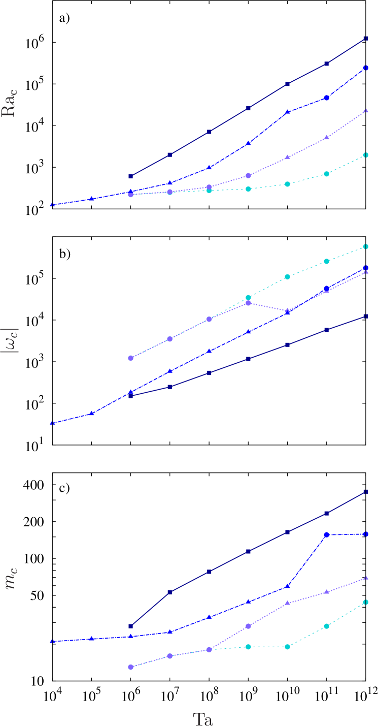
Figure 1: (a) Critical Rayleigh numbers ${\rm Ra_{c}}$, (b) critical drifting frequencies $|\omega_{c}|$ and (c) critical azimuthal wave number $m_{c}$ versus the Taylor number ${\rm Ta}$ for $\Pr=10^{-4},10^{-3},10^{-2},10^{-1}$ with dashed, dotted, dashed-dotted and solid line, respectively (Blue darkness increasing with $\Pr$ online). The symbols mean: $\bullet$ AP/SP mode, $\blacktriangle$ EA mode and $\blacksquare$ SC mode. This figure roughly explores the $({\rm Ta},\Pr)$ space as only few points are considered. Details for the interchange between EA and AP/SP modes (jumps in the figure) at $\Pr=10^{-3},10^{-2}$ are provided in Fig. 2.

Different types of instabilities have been found by varying the Taylor number in the range ${\rm Ta}\in[10^{4},10^{12}]$ for low and moderate Prandtl numbers $\Pr=10^{-4},10^{-3},10^{-2},10^{-1}$. The critical Rayleigh number, ${\rm Ra}_{c}$, drifting frequencies, $|\omega_{c}|$, and azimuthal wave number, $m_{c}$, are displayed versus ${\rm Ta}$ in Fig. 1 and Fig. 2. For the largest Prandtl number studied, $\Pr=0.1$, only spiralling columnar modes, with ${\rm Ra_{c}}=0.2{\rm Ta}^{0.57}$, become dominant (see Fig. 1(a)). This power law, coming from a fit to the points of the figure, is in close agreement with the results of Al-Shamali et al. (2004), obtained with $\Pr=1$ and non-slip boundary conditions also in thin spherical shells, and not so far from the leading order $2/3$ given by the asymptotic theories Roberts (1965); Busse (1970b); Dormy et al. (2004). In the case of $|\omega_{c}|$ (Fig. 1(b)) or $m_{c}$ (Fig. 1(c)) the agreement with the previous theories Roberts (1965); Busse (1970b); Dormy et al. (2004) is quite good giving $|\omega_{c}|={\rm Ta}^{0.34}$ and $m_{c}=4{\rm Ta}^{0.16}$. Spiralling modes always drift in the prograde direction.

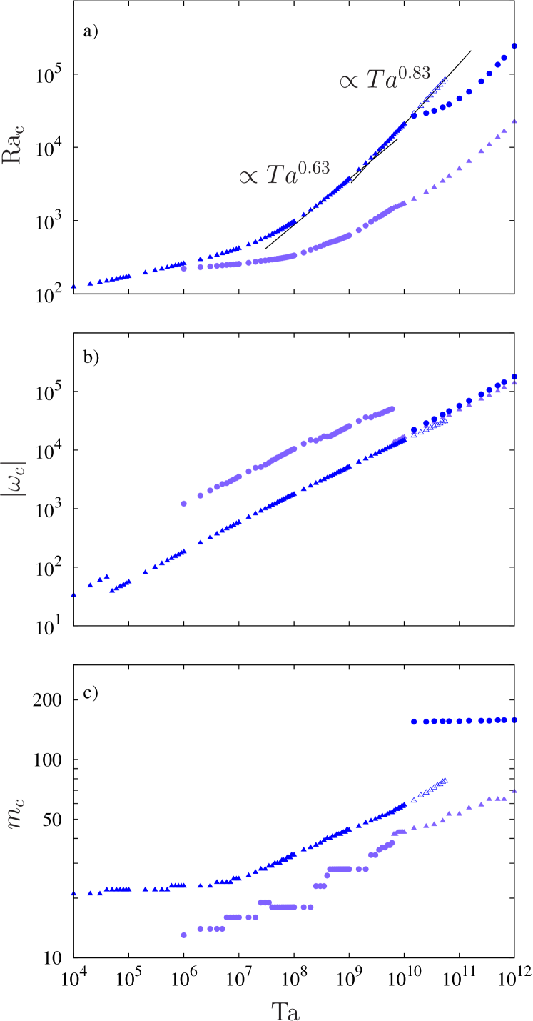
Figure 2: (a) Critical Rayleigh numbers ${\rm Ra_{c}}$, (b) critical drifting frequencies $|\omega_{c}|$ and (c) critical azimuthal wave number $m_{c}$ versus the Taylor number ${\rm Ta}$ for $\Pr=10^{-3},10^{-2}$ with light and dark grey (blue online), respectively. The symbols mean: $\bullet$ AP/SP mode and $\blacktriangle$ EA mode. Full/open points are used for dominant/nondominant modes. This figure shows in detail the ${\rm Ta}$ dependence and the interchange between EA and AP/SP modes found only at $\Pr=10^{-3},10^{-2}$ and roughly displayed in Fig. 1. In the case of $\Pr=10^{-2}$, nondominant EA modes ($\triangle$) are also displayed. The power law fits from the results are represented by a solid line.

The flow structure of the spiral columnar modes (SC) is displayed in the fourth row of contourplots shown in Fig. 3. The left group are for the temperature perturbation (from left to right: spherical, equatorial and meridional sections) and the right group are for the kinetic energy density ${\mathbf{v}}^{2}/2$. Notice in each section the black lines showing the position of the other two. The position of the spherical section is chosen to be close to a relative maximum. In the case of ${\mathbf{v}}^{2}/2$ it corresponds to the outer boundary. This figure shows that SC modes are equatorially symmetric and typically elongated in the axial direction (see the contour lines almost parallel to the vertical axis in the meridional section of ${\mathbf{v}}^{2}/2$), spiralling eastward in the azimuthal direction (slightly noticeable in each small cell of ${\mathbf{v}}^{2}/2$ in the equatorial section) and nearly tangent to the inner sphere. See also the 4th (from left to right) meridional section of the azimuthal velocity shown in Fig. 4.

Antisymmetric Polar (AP) mode
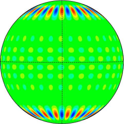
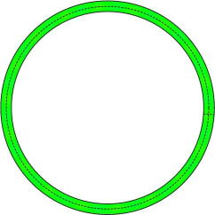
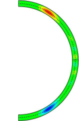
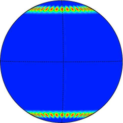
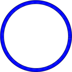
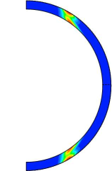
Symmetric Polar (SP) mode
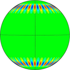
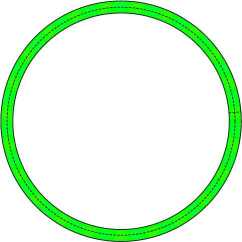
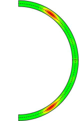
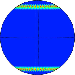
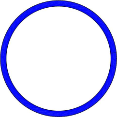
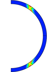
Equatorially Attached (EA) mode
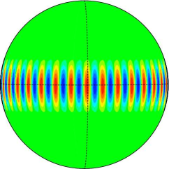
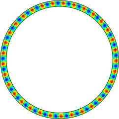
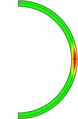
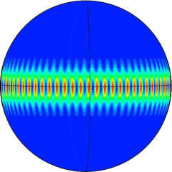
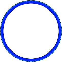
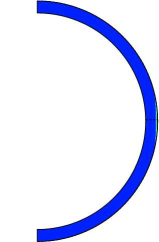
Spiralling Columnar (SC) mode
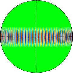
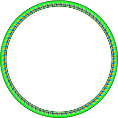
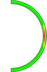
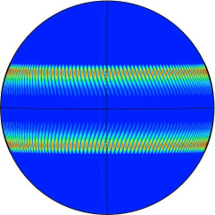
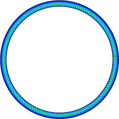
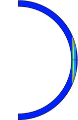
Antisymmetric Polar (AP) mode

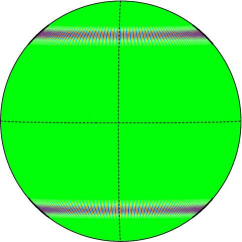
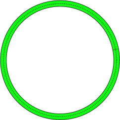
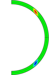
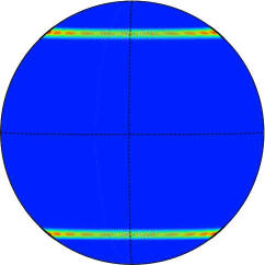
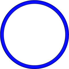
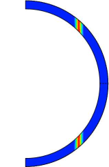
Figure 3: Spherical, equatorial and meridional sections of the temperature perturbation $\Theta$ (left) and of the kinetic energy density ${\mathbf{v}}^{2}/2$ (right) for the preferred modes of convection at $\Pr=10^{-3},{\rm Ta}=10^{8}$ with $m_{c}=18$ (1st row), $\Pr=2\times 10^{-3},{\rm Ta}=10^{8}$ with $m_{c}=23$ (2nd row), $\Pr=10^{-2},{\rm Ta}=10^{8}$ with $m_{c}=33$ (3rd row), $\Pr=10^{-1},{\rm Ta}=10^{8}$ with $m_{c}=78$ (4th row), and $\Pr=3\times 10^{-2},{\rm Ta}=10^{10}$ with $m_{c}=156$ (5th row). Color scale is not quantitative: $\Theta$: Red/blue means hottest/coldest fluid, respectively (green is for zero). ${\mathbf{v}}^{2}/2$: Red/blue means most/less energetic fluid, respectively. Contour plots of low azimuthal wave number SC, EA and AP modes can be found in Zhang (1992), Net et al. (2008) and Garcia et al. (2008), respectively.

AP	SP	EA	SC	AP

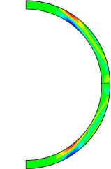
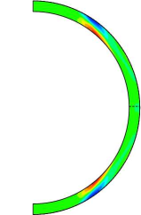
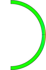
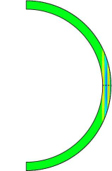
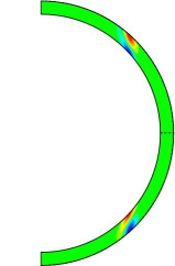
Figure 4: Meridional sections of the azimuthal velocity $v_{\varphi}$ for the preferred modes of convection at (from left to right) $(\Pr=10^{-3},{\rm Ta}=10^{8})$, $(\Pr=2\times 10^{-3},{\rm Ta}=10^{8})$), $(\Pr=10^{-2},{\rm Ta}=10^{8})$, $(\Pr=10^{-1},{\rm Ta}=10^{8})$, and $(\Pr=3\times 10^{-2},{\rm Ta}=10^{10})$. Color scale is not quantitative: Red/blue means positive/negative $v_{\varphi}$, respectively (green is for zero).

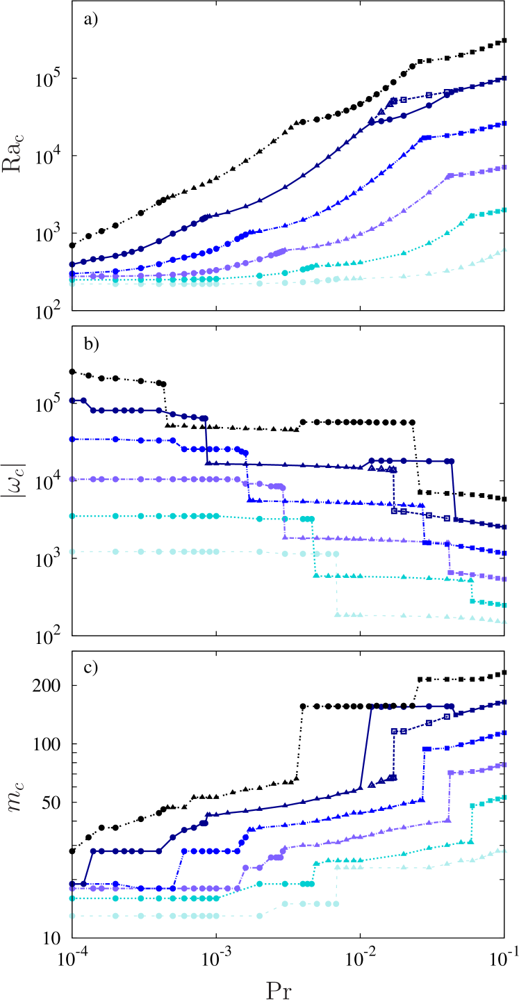
Figure 5: (a) Critical Rayleigh numbers ${\rm Ra_{c}}$, (b) critical drifting frequencies $|\omega_{c}|$ and (c) critical azimuthal wave number $m_{c}$ versus the Prandtl number $\Pr$ for ${\rm Ta}=10^{6},10^{7},10^{8},10^{9},10^{10},10^{11}$ (thin dashed, dotted, dashed-dotted, dashed-double-dotted, solid and double-dotted line style, respectively (blue darkness increases with ${\rm Ta}$ online)). The symbols mean: $\bullet$ AP/SP mode, $\blacktriangle$ EA mode and $\blacksquare$ SC mode. Full/open points are used for dominant/nondominant modes. The thick dashed line marks the transition between nondominant EA and SC modes at ${\rm Ta}=10^{10}$. This figure shows the tendency of AP/SP, EA and SC modes to be preferred at smaller $\Pr$ when ${\rm Ta}$ increases. For the largest ${\rm Ta}$, AP/SP modes are preferred at very small but also at relatively high $\Pr$.

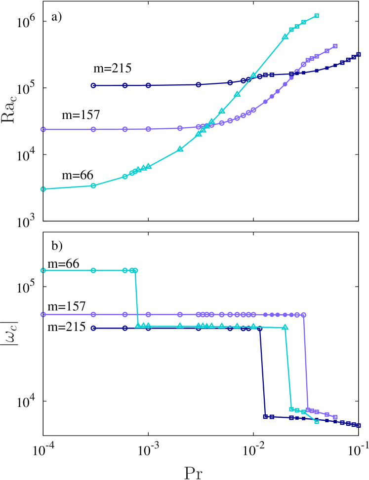
Figure 6: (a) Critical Rayleigh numbers ${\rm Ra_{c}}$ and (b) critical drifting frequencies $|\omega_{c}|$ versus the Prandtl number ${\rm Pr}$ for ${\rm Ta}=10^{11}$ and azimuthal wave numbers $m=66$, $m=157$ and $m=215$. The symbols mean: $\bullet$ AP/SP mode, $\blacktriangle$ EA mode and $\blacksquare$ SC mode. Full/open points are used for dominant/nondominant modes. While for $m=66$ the three types of modes are found, for $m=157,215$ only AP/SP or SC are obtained.

The situation is quite different for $\Pr=10^{-2}$ and $\Pr=10^{-3}$. In this case thermo inertial modes become preferred, which can be either equatorial (EA) Zhang and Liao (2004); Net et al. (2008); Sánchez et al. (2016) or polar (P) Garcia et al. (2008) depending on ${\rm Ta}$. This is shown in Fig. 2 where the critical parameters are plotted versus ${\rm Ta}$. At $\Pr=10^{-2}$ and ${\rm Ta}<1.25\times 10^{10}$ the instability takes the form of equatorial waves in which convection is nearly absent in the bulk of the fluid except for a very thin region near the outer surface at equatorial latitudes (see 3rd row of Fig. 3 or the 3rd (from left to right) meridional section of Fig. 4.). While for the lowest ${\rm Ta}$ the increasing of ${\rm Ra}_{c}$ is quite slow (see Fig. 2(a)), at ${\rm Ta}\in[10^{8},5\times 10^{9}]$ the power law fits well with ${\rm Ra_{c}}=0.008{\rm Ta}^{0.63}$, also found in Net et al. (2008) for the EA modes at $\Pr=0.005$ in a non-slip thick internally heated shell. From around ${\rm Ta}=5\times 10^{9}$ the ${\rm Ra_{c}}$ of EA modes follow a power law with a slightly larger exponent $\propto{\rm Ta}^{0.83}$ as found in Sánchez et al. (2016) for the EA modes in a stress-free sphere at the same $\Pr$ and up to ${\rm Ta}=10^{14}$. Nevertheless, the only difference observed between modes following the two different power laws is that at high ${\rm Ta}$ the patterns of $\Theta$ and $v_{r}$ are significantly more attached to the outer boundary.

Although at $\Pr=10^{-2}$ the modes are mostly prograde, for the lowest ${\rm Ta}$, retrograde waves have been found (see the jump in Fig. 2(b) at ${\rm Ta}=4\times 10^{4}$). This is typical and has been reported before for EA in thick shells. At ${\rm Ta}\in[10^{6},5\times 10^{9}]$ the variation of $|\omega_{c}|$ with ${\rm Ta}$ can be reasonably well approximated by $|\omega_{c}|=0.25{\rm Ta}^{0.48}$ while from ${\rm Ta}=5\times 10^{9}$ (i.e, when EA become non dominant) it is better to use $|\omega_{c}|\propto{\rm Ta}^{0.43}$. Both have an exponent a bit larger than predicted by asymptotic theories but in close agreement with the case of EA modes on a full sphere Sánchez et al. (2016).

The dependence of the critical azimuthal wave number $m_{c}$ displayed in Fig. 2(c) for the EA modes is a little bit lower than theoretical predictions, following $m_{c}=3{\rm Ta}^{0.13}$ in the interval ${\rm Ta}\in[10^{7},10^{10}]$. For lower ${\rm Ta}<10^{7}$, $m_{c}$ remains nearly constant while for ${\rm Ta}>10^{10}$ (where EA are non dominant) the exponent seems to increase to $m_{c}\propto{\rm Ta}^{0.18}$. At higher ${\rm Ta}>10^{11}$ the exponent found for EA modes in a full sphere was 0.25.

Surprisingly, and in contrast to what is found in full spheres, at ${\rm Ta}\approx 1.25\times 10^{10}$ EA modes are no longer preferred and either equatorially symmetric or antisymmetric polar modes, as in Garcia et al. (2008), are selected. Unlike the latter study with $\eta=0.4$, this antisymmetric modes have a very large $m_{c}$ and are dominant in a significantly larger interval ${\rm Ta}\in[1.5\times 10^{10},10^{12}]$. By comparing our results at $\eta=0.9$ with those of Garcia et al. (2008) at $\eta=0.4$ and those of Sánchez et al. (2016) at $\eta=0$, it seems that the thinner the shell, the more probable it is that AP or SP modes become dominant at high ${\rm Ta}$ and moderate $\Pr$. As it will be shown in the next section, AP or SP modes of relatively small azimuthal wave number are the most typical at low $\Pr$.

In the range explored ${\rm Ta}\in[1.25\times 10^{10},10^{12}]$ the critical azimuthal wave number of the polar mode remains almost unchanged $m_{c}\in[155,158]$ (see Fig. 2(c)) and the frequency follows $|\omega_{c}|\propto{\rm Ta}^{0.5}$. The dependence of ${\rm Ra}_{c}$ is not so clear and no power law can be fitted. When high azimuthal wave number AP or SP modes become preferred, convection is located in a narrow band parallel to the equator at very high latitudes, and ${\mathbf{v}}^{2}/2$ is almost $z$-independent. This is displayed in last row of Fig. 3 or the rightest meridional section of Fig. 4. The latter figure also shows the existence of a strong shear layer corresponding to a cone which is tangent to the inner sphere at latitudes close to $30^{\text{o}}$.

At $\Pr=10^{-3}$ inertial prograde modes also become preferred, but in this case EA modes are dominant at high ${\rm Ta}>6.13\times 10^{9}$ and AP or SP are dominant at low ${\rm Ta}<6.13\times 10^{9}$ (i.e the situation is reversed when compared with that at $\Pr=10^{-2}$). The transition can be clearly seen in the jump (from $|\omega_{c}|\approx 5\times 10^{4}$ to $|\omega_{c}|\approx 10^{4}$) of Fig. 2(b). At such small $\Pr$ the ${\rm Ra}_{c}$ increases slowly with ${\rm Ta}$. Only when EA modes become selected, does the dependence seem to approach to $\propto{\rm Ta}^{0.63}$, and $|\omega_{c}|$ is roughly $\propto{\rm Ta}^{0.5}$ in the whole ${\rm Ta}$ interval. The dependence of $m_{c}$ is of staircase type but globally is increasing slowly up to ${\rm Ta}\sim 10^{8}$, and beyond this with a slope $\propto{\rm Ta}^{0.18}$. While the patterns of convection of EA modes at $\Pr=10^{-3}$ are quite similar to those at $\Pr=10^{-2}$, those of AP or SP modes exhibit differences. The first noticeable difference is the azimuthal length scale (compare 1st/2nd with last row in Fig. 3). A second difference is that at $\Pr=10^{-2}$ the $z$-dependence of ${\mathbf{v}}^{2}/2$ is enhanced. This is not surprising because these polar modes are dominant at larger ${\rm Ta}$. In addition, at $\Pr=10^{-3}$ the modes are weakly multicellular (see spherical and meridional sections of $\Theta$) with convection present at larger latitudes and with shear layers extending from polar latitudes to close to the equator (see 1st/2nd plot (from left to right) of Fig. 4). Notice that there are no fundamental differences in the patterns of the AP and SP modes. For such a thin shell, any link between the high latitudes on both hemispheres practically disappears, and an AP mode can be obtained by azimuthally shifting an SP mode on one of the hemispheres.

Finally, at $\Pr=10^{-4}$ only SP or AP modes like those at $\Pr=10^{-3}$ are preferred up to ${\rm Ta}=10^{12}$. Up to ${\rm Ta}\approx 10^{8}$ there is almost no difference in the critical parameters between $\Pr=10^{-3}$ or $\Pr=10^{-4}$ (see Fig. 1). In addition, ${\rm Ra}_{c}$ starts to increase very slowly from ${\rm Ta}>10^{10}$ and no power law can be fit. Polar modes drift with very large (up to $10^{6}$) frequencies, that follow $|\omega_{c}|=1.5{\rm Ta}^{0.48}$. For such small $\Pr=10^{-4}$, the modes can be prograde but also retrogade as it happens for ${\rm Ta}=10^{9},10^{10}$ and $m_{c}=19$. The azimuthal wave number $m_{c}$ also starts to increase from ${\rm Ta}>10^{10}$ with $m_{c}=0.3{\rm Ta}^{0.18}$, i.e, with the same slope as for $\Pr=10^{-3}$ from ${\rm Ta}>10^{8}$ ((see Fig. 1(c)). Then, for the polar modes the large ${\rm Ta}$ limit (where $m_{c}$ starts to increase) seems to be reached at $\Pr{\rm Ta}^{1/2}\sim 10$.

IV Prandtl number dependence

According to the previous section, different types of modes may be preferred depending on $\Pr$. The aim of this section is to find the transitions between these modes in the parameter space $({\rm Ta},\Pr)$. To that end, further exploration by varying $\Pr$ is needed.

Figure 5 shows ${\rm Ra}_{c}$, $|\omega_{c}|$ and $m_{c}$ as a function of $\Pr\in[10^{-4},10^{-1}]$ for a set of 6 Taylor numbers from ${\rm Ta}=10^{6}$ to ${\rm Ta}=10^{11}$. In this figure the transition between spiralling, equatorial and polar modes can be identified by the cusps in the ${\rm Ra}_{c}$ curves (Fig. 5(a)) and jumps in the $|\omega_{c}|$ (Fig. 5(b)) or $m_{c}$ (Fig. 5(c)) curves. By increasing $\Pr$ from $10^{-4}$ there exist first one or several transitions among SP and AP modes for all ${\rm Ta}$ explored (some of them can be retrograde at $\Pr\sim 10^{-4}$). This is clearly noticeable from Fig. 5(c) in the jumps in each of the $m_{c}$ curves at the left of the plot. The convection patterns of these polar modes were described in previous section and are shown in the 1st (AP) and 2nd (SP) rows of Fig. 3 and in the 1st (AP) and 2nd (SP) plot of Fig. 4. For transitions between polar modes (either symmetric or antisymmetric) the jumps in $|\omega_{c}|$ are very small as are the cusps in ${\rm Ra}_{c}$.

The second transition, observed at a critical $\Pr$ number which tends to decrease with increasing ${\rm Ta}$, is between polar and equatorial modes. At the transition, $|\omega_{c}|$ decreases sharply by roughly one order of magnitude and ${\rm Ra}_{c}$ increases, with smaller slope. There exists also a jump in $m_{c}$, and the jump tends to decrease with ${\rm Ta}$.

For ${\rm Ta}\leq 10^{9}$ and larger $\Pr$ a third transition between EA and SC modes is found. As for the transition between SP/AP and EA modes, the critical $\Pr$ of this transition tends to decrease with increasing ${\rm Ta}$ although at a slightly slower rate. This transition is also characterised by a decrease of $|\omega_{c}|$ but is not so pronounced. When the new modes become preferred ${\rm Ra}_{c}$ increases at a lower rate, and they have a very small azimuthal length scale (seen as a big jump in $m_{c}$).

As mentioned in previous section, we have found very high azimuthal wave number polar modes preferred at moderate $\Pr$ and large ${\rm Ta}$. They are clearly dominant at ${\rm Ta}=10^{10},10^{11}$ around $\Pr=10^{-2}$ (see right top part of Fig. 5) and their region of stability tends to increase with ${\rm Ta}$. In the curve for ${\rm Ta}=10^{10}$ the transition between the non dominant EA and SC modes is shown (the open symbols on the right part of that curve). To visualise how these polar modes become dominant ${\rm Ra}_{c}$ and $|\omega_{c}|$ are plotted in Fig. 6 versus $\Pr$ for the azimuthal wave numbers $m=66,157,215$ at ${\rm Ta}=10^{11}$. While for $\Pr\in[10^{-4},10^{-1}]$ the $m=66$ mode can be polar, equatorial or spiralling (notice the two transitions in jumps of $|\omega_{c}|$), the $m=157,215$ modes only show a transition between AP/SP and SC modes. When decreasing $\Pr$ beyond the transition, ${\rm Ra}_{c}$ starts to decrease faster. The fact that the transition occurs at larger $\Pr$ for the $m=157$ polar mode allows it to be dominant.

We confirm the trend occurring in thicker shells. The smaller the $\Pr$ the smaller ${\rm Ra}_{c}$ and $m_{c}$ and the larger $|\omega_{c}|$. In the $\Pr$ interval explored, due to the multiple transitions, ${\rm Ra}_{c}$ cannot be fit by simple power laws. The drifting frequencies remain nearly constant for each type of mode, with the SC modes having a slightly steeper decrease. The dependence of $m_{c}$ with $\Pr$ can be approximated as roughly $\propto\Pr^{0.14}$ when ${\rm Ta}>10^{6}$ for the EA modes and $\propto\Pr^{0.2}$ for the SC modes and the larger $\Pr$. This contrast with the results on the full sphere Sánchez et al. (2016) where an exponent of $0.54$ was found for the EA modes.

V Transitions in the $({\rm Ta},\Pr)$ parameter space

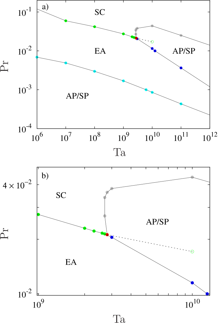
Figure 7: (a) Transitions between the different types of preferred modes (the points are obtained from Fig. 2 and Fig. 5 by means of linear interpolation). (b) Detail of (a) showing the triple point. The dashed line and the open circle mark the transition between nondominant EA and SC modes shown in Fig. 5.

From Fig. 2 and Fig. 5 and some additional computations, not shown in those figures, the locations of the different transitions in the $({\rm Ta},\Pr)$ parameter space have been obtained by linear interpolation, and the regions of stability of the different modes have also been roughly established. This is shown in Fig. 7 where the transitions from AP/SP to EA modes, from EA to SC modes, from EA to high $m$ AP/SP modes, and from high $m$ AP/SP to SC modes, correspond to the $4$ different curves containing cyan, green, blue and gray points, respectively. The general trend of this figure is that polar modes are preferred at very low $\Pr$, equatorial modes at moderate $\Pr$ and spiral modes at larger $\Pr$, but polar modes with high azimuthal wave number can also be preferred at moderate $\Pr$. As ${\rm Ta}$ is increased the position of the transitions tend to be located at lower $\Pr$. For instance we have obtained $\Pr_{\text{P/EA}}=0.68{\rm Ta}^{-0.29}$ (cyan points) and $\Pr_{\text{EA/SC}}=1.67{\rm Ta}^{-0.2}$ (green points), both power laws for ${\rm Ta}>10^{8}$. At approximately $({\rm Ta}_{3},\Pr_{3})=(2.8\times 10^{9},2.12\times 10^{-2})$ there is a transition between EA, AP and SC modes, giving rise to a triple Hopf bifurcation. At this point an equatorial, a polar and a spiralling mode have equal critical Rayleigh numbers within $1\%$ of precision (Table 1), i.e, of the same order of the spatial truncation errors. To the best knowledge of the authors this is the first time a triple point has been reported in the context of thermal convection in rotating spherical geometry. Choosing parameters near $({\rm Ta}_{3},\Pr_{3})$ will give rise to a very rich variety of travelling and modulated waves with very different azimuthal wave numbers, convective patterns and energy balances.

The region of stability of the high $m$ polar modes seems to widen with ${\rm Ta}$ making the region of stability of equatorial modes thinner. By extrapolating the EA/SC transition curve to larger ${\rm Ta}>10^{12}$ (by continuing the dashed line through the empty circle and so on in Fig. 7) one might expect the EA/SC transition curve to appear again, arising at another triple point. This is likely to happen because the slope of the P/SC transition curve seems to be larger than that of the EA/SC modes. A similar argument can be applied to conclude that the region of equatorial modes confined between the two regions of polar modes will probably disappear, so that at some fixed ${\rm Ta}>10^{12}$ there will exist only 3 types of modes when $\Pr$ is varied, namely (from low to large $\Pr$) AP/SP, EA and SC modes. An interesting question then arises: could it be that for some ${\rm Ta}>10^{12}$ high wave number AP/SP modes become preferred again between EA and SC modes?

	Type		$m_{c}$	${\rm Ra}_{c}$	$\omega_{c}$
	EA		$57$	$2.5564\times 10^{4}$	$-7.6968\times 10^{3}$
	SC		$92$	$2.5662\times 10^{4}$	$-2.6474\times 10^{3}$
	AP		$154$	$2.5699\times 10^{4}$	$-9.6376\times 10^{4}$

Table 1: Critical parameters for equatorial, spiralling and polar modes of convection at ${\rm Ta}=2.8\times 10^{9}$ and $\Pr=2.12\times 10^{-2}$. The differences between all ${\rm Ra}_{c}$ are less than $1\%$ (assumed for spatial resolution errors). Then, at this $({\rm Ta},\Pr)$ an AP, EA and SC mode are preferred at the same time.

VI Application to convection in stars and stellar oceans

For the sake of curiosity, the critical parameters of the onset of convection for three different type of astrophysical applications will be estimated in the following with the help of the power law scalings obtained in previous sections. They are:

• Spiralling modes: ${\rm Ra_{c}}\sim 0.2{\rm Ta}^{0.57}$, $|\omega_{c}|\sim{\rm Ta}^{0.34}$ and $m_{c}\sim 4{\rm Ta}^{0.16}$.

• Equatorial modes: ${\rm Ra_{c}}\sim 0.008{\rm Ta}^{0.63}$, $|\omega_{c}|\sim 0.25{\rm Ta}^{0.48}$ and $m_{c}\sim 3{\rm Ta}^{0.13}$.

• Polar modes: $|\omega_{c}|\sim 1.5{\rm Ta}^{0.48}$ and $m_{c}\sim 0.3{\rm Ta}^{0.18}$ for $\Pr{\rm Ta}^{1/2}>10$.

In addition, the type of instability (SC,EA or P) can be predicted using $\Pr_{\text{P/EA}}=0.68{\rm Ta}^{-0.29}$ and $\Pr_{\text{EA/SC}}=1.67{\rm Ta}^{-0.2}$ obtained in § V. The Taylor number, ${\rm Ta}=\Omega^{2}d^{4}/\nu^{2}$, and Prandtl number, $\Pr=\nu/\kappa$, come from values of physical properties (see Table 2) obtained in previous studies, details of which are given below. We also estimate the period of the waves from $P=(2\pi m_{c}/|\omega_{c}|)d^{2}/\nu$ in seconds. Recall that negative frequencies give positive drifting (phase) velocities $c=-\omega_{c}/m_{c}$ and the waves drift in the prograde direction.

At this point, it is worth mentioning the applicability of these results to stellar convection. In our Boussinesq model, density variations are neglected, except in the buoyancy term. This is far from stellar conditions, where the scale height of density variations Spiegel and Veronis (1960) can be three orders of magnitude smaller than the gap width of the convective layer. However, this simplification can be justified when the focus is to study the basic but relevant mechanisms of rotation, buoyancy and thin spherical geometry, and their interconnections.

In addition, it is often stated that qualitative dynamical properties of Boussinesq flows are inherited by compressible flows at the same parameter conditions, provided the velocities remain subsonic. For instance, quite similar large scale two vortex turbulent structures have been found in Chen and Glatzmaier (2005) in a rectangular box both with and without strong stratification, in both cases with kinetic energy scaling as $k^{-3}$ ($k$ is the Kolmogorov wave number). In the specific case of rotating spherical shells, the linear theory of anelastic convection was formulated in Jones et al. (2009). They found that with stratification, convection tends to be moved to near the outer shell with larger ${\rm Ra_{c}}$, $m_{c}$ and $|\omega_{c}|$ for $\Pr=0.1,1,10$. Specifically, with the strongest stratification, $\rho_{r_{i}}/\rho_{r_{o}}\approx 150$, the critical parameters increase, with respect to the Boussinesq case, by around an order of magnitude in the worse case. With these considerations, the linear theory of Boussinesq convection may be used to obtain reasonable bounds for the critical parameters for compressible flows in a regime where the compressible formulation is still numerically unfeasible. Further support for this result is given in Calkins et al. (2015). The same scaling laws for the critical parameters, in both Boussinesq and compressible linear analysis, are valid in the limit of large rotation in a rotating plane layer geometry with very low $\Pr$. As the authors of Calkins et al. (2015) stated in their study, further research at the very low $\Pr$ number regime is needed. Recently Wood and Bushby (2016), also in a rotating plane layer geometry, found restrictions on the Boussinesq approximations at very low $\Pr$. In this study, asymptotic scalings for the Boussinesq and compressible onset of convection were compared with numerical computations of the compressible case. For a perfect gas, with moderate ratio between the domain and the temperature scale heights, differences of less than one order of magnitude in ${\rm Ra}_{c}$ were found between the two approximations, at $\Pr=10^{-4}$.

Although convection in stars is believed to be fully turbulent Brummell and Toomre (1995); Brandenburg et al. (2000), the analysis of the onset of convection is worthwhile because patterns and characteristics at the onset may be able to persist even in strongly nonlinear regimes. This was argued to happen in Landeau and Aubert (2011) even in the case of nondominant inertial and axisymmetric modes. A previous study Garcia et al. (2014b) also suggests that the mean period of a fully developed turbulent solution does not change drastically from that of the onset of convection. In that study at $\Pr=0.1$, the frequency spectrum of time series from turbulent solutions that are 100 times supercritical have a maximum peak at a frequency roughly 3 times larger than the corresponding value at the onset of convection.

Property	Sun(1)	Accreting white	Accreting neutron	Molecular region
		dwarf ocean(2)	star ocean(3)	Jupiter(4)
$\kappa$ (cm2s-1)	$10^{7}-10^{9}$	$10^{1}-10^{5}$	$10^{6}$	$10^{-5}$
$\nu$ (cm2s-1)	$10^{0}-10^{4}$	$10^{-4}-10^{-2}$	$10^{6}$	$10^{-6}$
$d$ (cm)	$10^{10}$	$10^{8}$	$10^{3}-10^{4}$	$10^{8}$
$\Omega$ (s-1)	$2.6\times 10^{-6}$	$7\times 10^{-5}$	$10^{2}$	$2\times 10^{-4}$

Table 2: Physical parameters of three example astrophysical convection scenarios. Jupiter is included for comparison purposes. Thermal diffusivity $\kappa$, kinematic viscosity $\nu$, layer width $d$ and rotation rate $\Omega$. Values are taken: (1) from Brandenburg et al. (2000) and the references therein. (2) from Nandkumar and Pethick (1984); Garaud et al. (2015); Isern et al. (2017). (3) from Yakovlev and Urpin (1980); Nandkumar and Pethick (1984); Watts (2012). (4) from Bagenal et al. (2004); Showman et al. (2011)

For illustration, we shall now consider a selection of different astrophysical scenarios where convection is important, to assess how the results of our study would apply. Shell or envelope convection can arise in many different astrophysical scenarios. Low mass main sequence stars burning hydrogen to helium in their cores, for example, are expected to have convective zones in their envelopes. In Section VI.1 we consider this scenario and look at the parameter space appropriate to the Sun. Shell convection can also occur during post main sequence evolution, via shell burning or as elements heavier than hydrogen are burned. This may occur on the Red Giant Branch, Horizontal Branch, and Asympotic Giant Branch (see for example Herwig et al. (2006); Meakin and Arnett (2007); Mocák et al. (2009); Kippenhahn et al. (2013)). We do not examine these scenarios in this paper, but note them for reference. White dwarfs can also develop convection in various ways. Isolated white dwarfs develop convective zones as they cool, and we examine this scenario in Section VI.2. Accreting white dwarfs and neutron stars can also develop convective zones as accreted material from a companion star undergoes thermonuclear burning. When this burning is unstable, this can manifest in bright transient bursts: classical novae on accreting white dwarfs, and Type I X-ray bursts on accreting neutron stars. We do not study the convective zones of accreting white dwarfs further in this paper, but refer the interested reader to, for example, Shankar et al. (1992); Glasner and Livne (1995); Kercek et al. (1999); Starrfield et al. (2016). However in Section VI.3 we consider the parameter space appropriate for accreting neutron star oceans.

VI.1 Sun

For convection occurring in the Sun (Miesch (2000); Paternò (2010) provide good reviews focusing on the role of rotation), kinematic viscosities range from $\nu=1$ cm²s^-1 near the surface to $\nu=10^{4}$ cm²s^-1 in the deeper layers, due to radiative viscosity (see Brandenburg et al. (2000) and the references therein). This gives rise to very low Prandtl numbers $\Pr\in[10^{-9},10^{-3}]$ and, depending on the size $d$ of the convective layer, to quite large Rayleigh numbers ${\rm Ra}\in[10^{18},10^{24}]$ (see Sec. 2.4 of Gilman (2000), Sec. 2.3 of Brun et al. (2015) or Hanasoge et al. (2016)). By assuming a size $d=10^{10}$ cm ($\eta>0.8$) Brandenburg et al. (2000), one expects ${\rm Ta}\in[10^{21},10^{29}]$. Our predictions are shown in Table 3. According to this table, given the low Prandtl number of the Sun, the most probable type of mode is equatorial. This type of Boussinesq solar convection was first studied in Busse (1970a) by considering only the radial dependence for small amplitude convection at small ${\rm Ta}$. Recent studies on solar convection in the context of rotating spherical shells incorporate more complex physics by using the anelastic approximation Glatzmaier (1984). More realistic parameters (${\rm Ta}=10^{6}$ and $\eta\approx 0.7$) have been considered in Miesch et al. (2000), and weak lateral entropy variations at the inner boundary have been imposed in Miesch et al. (2006). Nevertheless, they are restricted to moderate $\Pr\sim 0.1$. According to our results, and assuming the lowest $\Pr<10^{-6},$ it is also possible that polar modes become preferred, or at least become relevant when nonlinearities are included.

At this point it is interesting to see which time scales come from our results at the above estimated range of ${\rm Ta}$. Considering an equatorial mode, a long timescale, $P\sim 10^{3}-10^{4}$ years, is obtained. In the case of polar modes, the timescale is a little bit shorter, at $10^{2}-10^{4}$ years. These orders of magnitude estimates are not dissimilar to the long term variability timescales of the Sun, the Gleissber and Suess (also named the de Vries) cycles of $50-140$ years and $170-260$ yrs, respectively Ogurtsov et al. (2002), an unnamed $500$ and $1000$ yrs cycle and the Hallstatt cycle ($2300$ years) Kern et al. (2012), or the evidence of millenial periods of $6000$ yrs Xapsos and Burke (2009) and $9500$ years Sánchez-Sesma (2016) suggested recently. Notice the robustness of the predictions: although ${\rm Ta}$ spans 8 orders of magnitude, the periods obtained vary by only 2 orders of magnitude. Many of the principal features of the well-known 11-year Schwabe period can basically be explained in terms of dynamo theory Parker (1955); Choudhuri et al. (2007). However, its origin is still not well understood because the fields are strongly influenced by rotation and turbulent convection Strugarek et al. (2017). Moreover, the long-term solar-activity variation described above imposes several constraints on current solar dynamo models (either deterministic or including chaotic drivers). See the very recent review Usoskin (2017) Sec. 4.4 for further details. Because convection is believed to be the main driver of natural dynamos Dormy and Soward (2007), and the different dynamo branches first bifurcate from purely convective flows, the time scales predicted from our results may be present in dynamos bifurcated from convective flows at similar range of parameters. Simulating such self-excited dynamos at the parameter regime covered in our study is still numerically unattainable.

Type of mode	Property	Sun	Accreting white	Accreting neutron
			dwarf ocean	star ocean
	${\rm Ta}$	$10^{21}-10^{29}$	$10^{28}-10^{32}$	$10^{4}-10^{8}$
	$\Pr$	$10^{-9}-10^{-3}$	$10^{-9}-10^{-3}$	$10^{1}-10^{2}$
	$\Pr_{\text{P/EA}}$	$10^{-9}-10^{-6}$	$10^{-10}-10^{-8}$	$10^{-3}-10^{-1}$
	$\Pr_{\text{EA/SC}}$	$10^{-6}-10^{-4}$	$10^{-6}-10^{-5}$	$10^{-2}-10^{0}$
	${\rm Ra_{c}}$	$10^{11}-10^{16}$	$10^{15}-10^{17}$	$10^{3}-10^{6}$
	$|\omega_{c}|$	$10^{7}-10^{10}$	$10^{9}-10^{11}$	$10^{0}-10^{1}$
SP	$m_{c}$	$10^{4}-10^{5}$	$10^{5}-10^{6}$	$10^{0}-10^{1}$
	$P$)(years)	$10^{6}-10^{9}$	$10^{7}-10^{8}$	$10^{-8}-10^{-6}$
	${\rm Ra_{c}}$	$10^{11}-10^{16}$	$10^{15}-10^{18}$
	$|\omega_{c}|$	$10^{9}-10^{13}$	$10^{13}-10^{14}$
EA	$m_{c}$	$10^{3}-10^{4}$	$10^{4}$
	$P$ (years)	$10^{3}-10^{4}$	$10^{2}-10^{3}$
	${\rm Ra_{c}}$
	$|\omega_{c}|$	$10^{10}-10^{14}$	$10^{13}-10^{15}$
P	$m_{c}$	$10^{3}-10^{4}$	$10^{4}-10^{5}$
	$P$ (years)	$10^{2}-10^{4}$	$10^{2}-10^{3}$

Table 3: Estimation of the critical parameters and a typical time scale $P=(2\pi m_{c}/|\omega_{c}|)d^{2}/\nu$ in seconds (this is the timescale associated with the drifting phase velocity as computed in the rotating frame) for the Sun, a white dwarf and a neutron star depending on the type of mode, spiralling (SC), equatorial (EA) or polar (P). In the case of neutron stars only SC modes are considered since they are the only ones that can be preferred for the range of parameters. For the Sun and the white dwarf scenario considered, all of them could be preferred depending on appropriate particular choice of $\Pr$. This is indicated by the critical $\Pr$ at the P/EA and EA/SC transitions, which are also shown.

VI.2 Cooling White Dwarfs

White dwarfs are highly degenerate, except in a thin layer close to the surface. The idea that cooling white dwarfs may have a convective mantle is a long-established one (see for example Schatzman (1958); Fontaine and van Horn (1976); Tremblay et al. (2013)). Very recently,  Isern et al. (2017) suggested that associated dynamo action might explain the magnetic field observed in isolated white dwarfs. The authors focused on a heavy ($1.0M_{\odot}$) white dwarf because magnetic white dwarfs are typically observed to be more massive. Here we consider a cooling white dwarf with properties similar to the one studied in that paper, noting however that convective envelopes of white dwarfs could occupy a much wider range of parameter space.

Following Nandkumar and Pethick (1984) a kinematic viscosity of $\nu=3.13\times 10^{-2}$ cm²s^-1 was used in Isern et al. (2017). We consider the range $\nu=10^{-4}-10^{-2}$ cm²s^-1 of possible viscosities, take $d=10^{8}$cm as the size of the convective layer (see Figure 1 of Isern et al. (2017)), and a total stellar radius roughly $R=5\times 10^{8}$cm for our estimations. These values give rise to $\eta\approx 0.8$. However, as the white dwarf cools, the size of the convective layer decreases towards zero, giving rise larger values of $\eta$. Although periods of white dwarfs range from hours to days or longer Kawaler (2004), we assume a period of one day. Results are shown in table 3. As in the case of the Sun, the expected low Prandtl number makes equatorial modes more feasible, but polar modes are also possible. Convection sets in at a critical Rayleigh number $10^{15}-10^{18}$, with drifting periods $\sim 10^{2}-10^{3}$ years. Further work would be required to investigate the potential consequences.

VI.3 Accreting Neutron Stars

The case of convection in very thin oceans of accreting neutron stars covers quite a different region in Ta, Pr parameter space compared to the Sun and white dwarfs. Neutron stars typically have radii $\sim 10$ km and rotation rates up to $\lesssim 1$ kHz. Accreting neutron stars build up very thin oceans (which are, in the zones where burning and convection occur, composed primarily of hydrogen, helium and carbon) with $d<10^{4}$ cm, making the aspect ratio very large $\eta=r_{i}/r_{o}\geq 0.999$. Convection is expected to be triggered due to thermonuclear burning of the accreted material, which can take place in an unstable fashion due to the extreme temperature dependence of the nuclear reactions, giving rise to the phenomenon of Type I X-ray bursts (see Strohmayer and Bildsten (2006) for a general review of Type I X-ray bursts and Malone et al. (2011, 2014); Keek and Heger (2017) for more specific discussions of convection). Surface patterns known as burst oscillations are observed to develop frequently during thermonuclear bursts, motivating our interest in convective patterns Watts (2012). Due to the high densities of matter in the neutron star ocean, the main contribution to microphysics is from highly degenerate electrons. The heat capacity can be estimated using the formula for a degenerate gas of fermions: $c_{P}=(\pi^{2}k_{b}/2\mu_{e}m_{p})k_{b}T/E_{F}\sim 10^{8}$ ergs g^-1 K^-1Hook and Hall (1991). Conductivity, $K\sim 10^{16}$ ergs cm^-1 s^-1 K^-1 , and kinematic viscosity, $\nu\sim 10^{6}$ cm²s^-1, are estimated from expressions in Yakovlev and Urpin (1980); Nandkumar and Pethick (1984), thus the Prandtl number is of the order $\Pr\sim 10^{2}$. These high viscosities and extremely thin convective layers combine to ensure that the Taylor number is not so high, ranging from ${\rm Ta}=10^{8}$ for $d=10^{4}$ cm (the expected ignition depth for Carbon), and ${\rm Ta}=1$ for $d=10^{2}$ cm (the expected ignition depth for hydrogen/helium). The full accreted ocean extends to a depth of a few times $10^{4}$ cm. Given this range of possible values for ${\rm Ta}$, very different flow regimes might be expected, and further research is needed into the physical conditions of neutron star oceans (our current study does not fully cover this range of parameter space). In what follows, and in Tables 2 and 3, we discuss a more restricted range ${\rm Ta}\in[10^{4},10^{8}]$, so as not to extrapolate too far beyond the bounds our study.

If we assume $\Pr=10^{2}$ and ${\rm Ta}\in[10^{4},10^{8}]$ to be the valid regime of a neutron star ocean, it is clear from extrapolating Fig. 7 that the preferred mode of convection will be SC. The $\Pr$ values are beyond the range covered in our study, however the numerical computations of Zhang (1992) just fall in to the neutron star regime, albeit in a thicker shell (geometric effects are believed to be of secondary importance with respect to $\Pr$). At $\Pr=10^{2}$ these authors obtained following power laws: ${\rm Ra_{c}}=1.99{\rm Ta}^{0.66}$, $|\omega_{c}|=0.0190{\rm Ta}^{0.33}$ and $m_{c}=0.0687{\rm Ta}^{0.16}$ if we use the analytic formulas, and ${\rm Ra_{c}}=4.057{\rm Ta}^{0.66}$, $|\omega_{c}|=0.0683{\rm Ta}^{0.33}$ and $m_{c}=0.0819{\rm Ta}^{0.16}$ if we use the numerical values at ${\rm Ta}=10^{8}$ given in Table 2 of Zhang (1992) (it should be noted that the definition of ${\rm Ta}$ used in Zhang (1992) is different to the one used here). Then, ${\rm Ra_{c}}\sim 10^{3}-10^{6}$, $|\omega_{c}|\sim 10^{0}-10^{1}$ and $m_{c}\sim 10^{0}-10^{1}$, which gives rise to a period $P\sim 1-10$ s.

One of the less well understood phenomena occuring on neutron stars are burst oscillations (for a review see Watts (2012)). These occur on accreting neutron stars in the aftermath of a Type I X-ray burst, and are observed as modulation of the X-ray luminosity at a frequency very close to that of the spin frequency, sometimes drifting by up to a few Hz in the tail of a burst as the ocean cools. They are caused by pattern formation in the burning ocean. Currently the two leading explanations of this phenomena involve flame spreading Spitkovsky et al. (2002); Cavecchi et al. (2013, 2015, 2016); Mahmoodifar and Strohmayer (2016), or global modes of oscillation of the ocean Heyl (2004); Piro and Bildsten (2005), but no model yet fits the data precisely, and both mechanisms may be involved. Convection is expected to occur in many bursts, however, and the possible role of convection in pattern formation has yet to be fully investigated. With a rotating frame frequency of 0.1 - 1 Hz, the timescales associated with the convective patterns computed above are certainly compatible with those required to explain burst oscillations (where a small rotating frame frequency would required to keep the observed frequency within a few Hz of the spin frequency).

It should be noted that in these computations we have only accounted for temperature differences, and do not take into account burning physics or compositional gradients. This would not affect estimated dimensionless parameters $\Pr,{\rm Ta}$ but does mean that there is much work to do before direct comparison with astrophysical phenomena since non-linear effects would become relevant. To illustrate more easily the parameter regime into which the astrophysical scenarios mentioned above fall, Fig. 8(a) and (b) highlight the region occupied by each (in $(1-\eta,{\rm Ta})$ and $(\Pr,{\rm Ta})$ parameter space, respectively), together with the region covered by current and previous numerical studies. In addition, Fig. 8(b) includes the region of preference of each convective instability AP/SP, EA, and SC extrapolated from Fig. 7. While the Sun and white dwarfs have aspect ratios $\eta$ that are numerically attainable, they have ${\rm Ta}$ numbers which are impossible to handle with current simulations. The latter does not occur in the case of neutron stars, but in contrast, very thin layers, demanding prohibitive spatial resolutions, must be considered.

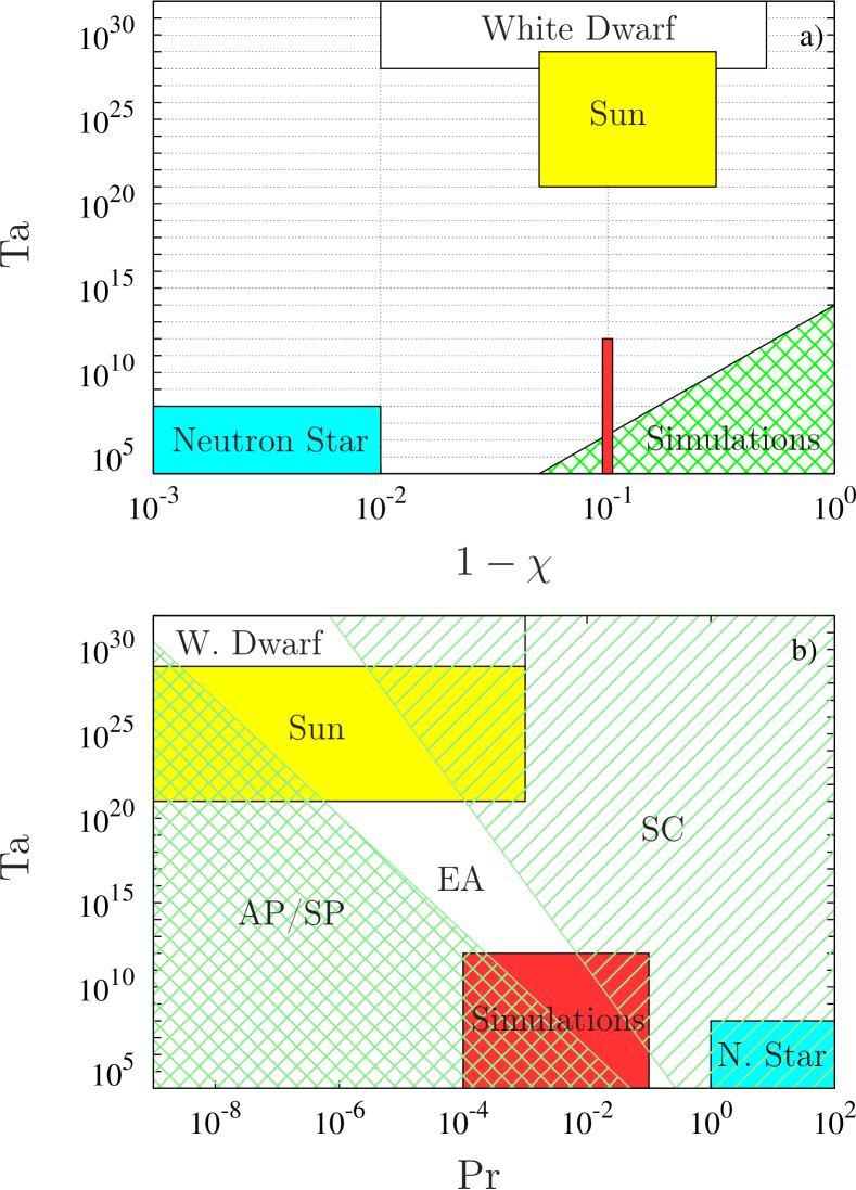
Figure 8: a) Estimates of ${\rm Ta}$ and $1-\chi$ for stars convective oceans and parameter values of the current (red) and previous (green) numerical studies of thermal convection which are clearly still far from stellar conditions. b) Same as a) but for ${\rm Ta}$ and $\Pr$. The estimated region of stability of the different convective instabilities SC (with stripes), EA (plain) and AP/SP (cross-hatched) is also shown.

VII Conclusions

The onset of low Prandtl number Boussinesq thermal convection in fast rotating very thin spherical shells is investigated carefully in this paper, by means of detailed numerical computations. A massive exploration of the parameter space $({\rm Ta},\Pr)$ is performed in a range of astrophysical interest characterised by low $\Pr$ and high ${\rm Ta}$ and very thin spherical shell $\eta=0.9$ with stress-free conditions. The use of efficient time integration methods has been useful for integrating the short temporal scales exhibited by the flows at high ${\rm Ta}$ and low $\Pr$. The parallelism of the code allows us to cope with the high resolutions needed to follow the marginal stability curves for a wide range of azimuthal wave numbers $m\in[10,500]$. This is necessary because the curves of quite different $m$ are very close in the case of very thin shells. In comparison with previous linear numerical studies in such thin ($\eta>0.8$) geometry Al-Shamali et al. (2004), the present study considers several orders of magnitude larger ${\rm Ta}$ and smaller $\Pr$ numbers. The region of the parameter space covered is even wider than most of the linear studies in thicker shells. Such very low $\Pr$ and large ${\rm Ta}$ number have previously been reached only in the recent numerical Sánchez et al. (2016) and analytic Zhang et al. (2017) studies, and then only for the case of a full sphere.

A first exploration at four fixed $\Pr<1$ reveals the existence of three types of preferred modes as ${\rm Ta}$ is varied. Prograde spiralling columnar (SC) convection occurs at larger $\Pr$ and the power laws obtained for the critical parameters agree quite well with previous results. For intermediate $\Pr$, equatorial (EA) modes, which can be retrograde for small ${\rm Ta}$, are found to be consistent with former studies considering thicker shells but, surprisingly, prograde equatorial antisymmetric or symmetric polar (AP/SP) modes with high wave number can also dominate at $\Pr=10^{-2}$ and ${\rm Ta}=10^{12}$. The latter type of modes are the only ones preferred at the lowest $\Pr=10^{-4}$, but in this case they can also be retrograde and show multicellular structures and strong shear layers which extend in the latitudinal direction. Antisymmetric polar modes, with convection confined inside the inner cylinder, were found for first time in Garcia et al. (2008) considering a shell with $\eta=0.4$, but they are dominant in a substantially smaller range of ${\rm Ta}$ when compared with our results at $\eta=0.9$. The latter fact increases the relevance of polar antisymmetric convection since low Prandtl number fluids convecting in very thin shells are common in stellar interiors.

With further exploration, by varying $\Pr$, the transitions among SC, EA and AP/SP modes are computed and traced in the $({\rm Ta},\Pr)$ space. This is the first time that this has been done: previous studies Ardes et al. (1997); Net et al. (2008) provided only a qualitative sketch in a smaller parameter region. At the lowest $\Pr$ values, polar modes become the only ones that are preferred and the critical parameters become nearly constant, suggesting the zero-Prandtl-limit is not far. The transition between AP/SP and EA modes takes place at $\Pr_{\text{P/EA}}=0.68{\rm Ta}^{-0.29}$, giving rise to a sharp step in the drifting frequency $|\omega_{c}|$ and a jump in $m_{c}$. The step and the jump tend to decrease with ${\rm Ta}$. Equatorial modes are superseded by SC at $\Pr_{\text{EA/SC}}=1.67{\rm Ta}^{-0.2}$ but only for ${\rm Ta}<2.8\times 10^{9}$. The transition between EA and SC modes is also characterised by a sharp step in the drifting frequency $|\omega_{c}|$ and a big jump in the azimuthal wave number.

At larger ${\rm Ta}$ and moderate $\Pr$ we have found two additional transitions not described previously. One is between EA and AP/SP modes and the other is between AP/SP and SC modes, taking place at larger $\Pr$. The frequencies $|\omega_{c}|$ are slightly increased for the former but strongly decreased for the latter. The situation for $m_{c}$ is different: it increases substantially when AP/SP polar modes become selected but only slightly when SC overcomes the AP/SP modes. The two transition curves intercept at $({\rm Ta}_{3},\Pr_{3})=(2.8\times 10^{9},2.12\times 0^{-2})$ giving rise to a triple-point bifurcation that, to the best knowledge of the authors, has never been reported before in the context of thermal convection in rotating spherical geometry. At this triple-point, AP/SP, EA and SC modes are dominant and have very different $|\omega_{c}|$ and $m_{c}$. This is relevant because when nonlinearities are included, a rich variety of chaotic dynamics may be expected almost at the onset. In addition, as the three types of modes are characterised by different physical mechanisms, nonlinear solutions driven by different force balances are expected to coexist at the triple-point. The study of the associated zonal flows and the magnitude of any differential rotation that arise in these different nonlinear regimes is important for the understanding of stellar ocean convection.

Finally, the fit formulae computed are used to estimate the critical parameters, the characteristic time scales and the most likely mode for the onset of convection occurring in the Sun, white dwarfs and accreting neutron stars. Although Boussinesq thermal convection in thin rotating spherical shells fails to reproduce the compressibility effects in stellars fluids, it captures the essential features of rotation and spherical geometry and thus gives valuable insight for further studies of more realistic models. Using known values of the physical properties, reasonable results for the critical Rayleigh number and the time scales are achieved, which are of similar order to observational phenomena reported in the literature.

According to our results equatorial modes (and polar modes with less degree) are the best candidates in the case of Sun and cooling white dwarf convection because of their low $\Pr$. Their time scales are about $10^{2}-10^{4}$ years for the Sun, encompassing the well-known long term periods Gleissber and Suess or Hallstatt cycles, and slightly lower at ($10^{2}-10^{3}$) years for white dwarfs. In the case of accreting neutron star oceans the situation seems to be quite different. It is not clear which regime they will belong to, because they have very viscous (electron degeneracy) fluids. Our results suggest ${\rm Ta}=10^{0}-10^{8}$ depending on the size of the shell considered and $\Pr=10^{2}$. If we assume ${\rm Ta}>10^{3}$ then convection will take the form of spiralling columns drifting very rapidly (on time scales of $1-10$ seconds). These timescales are consistent with some of the timescales seen in thermonuclear bursts where the accreted ocean develops patterns known as burst oscillations, and may therefore be of interest to studies of this as yet unexplained phenomenon.

Erratum: The onset of low Prandtl number thermal convection in thin spherical shells [Phys. rev. Fluids 3, 024801 (2018)]

Property	Accreting neutron
	star ocean
$\kappa$ (cm2s-1)	$10^{3}-10^{5}$
$\nu$ (cm2s-1)	$10^{0}$
$d$ (cm)	$10^{2}-10^{4}$
$\Omega$ (s-1)	$10^{2}$

Table 4: Physical parameters corresponding to an accreting neutron star ocean. Thermal diffusivity $\kappa$, kinematic viscosity $\nu$, layer width $d$ and rotation rate $\Omega$. Values are taken from Yakovlev and Urpin (1980); Nandkumar and Pethick (1984); Watts (2012).

We have performed the linear stability analysis in thin rotating spherical shell thermal convection models at low Prandtl number. The results have been used to extrapolate to several astrophysical scenarios, namely, the sun, cooling white dwarfs and accreting neutron stars. Unfortunately there was an error in the estimation of the kinematic viscosity for the case of accreting neutron star oceans, which we correct here. This erratum concerns only a small part of the paper in Sec. VI involving one column in Tables II and III, and Fig. 8. The changes are discussed in the following.

Tables 4 and 5 (corresponding to Tables II and III of the original paper) provide the correct values for the accreting neutron star ocean scenario. A valid estimation for the kinematic viscosity $\nu$ is $\nu\sim 1$ cm² s^-1 rather than $\nu\sim 10^{6}$ cm² s^-1 stated in the original paper. The new value of $\nu$, and slightly amended values for the thermal conductivity $\kappa=10^{3}-10^{5}$ cm² s^-1 and gap width $d=10^{2}-10^{4}$ cm ($\kappa=10^{6}$ cm² s^-1 and $d=10^{3}-10^{4}$ cm were supposed in our paper) give rise to new estimations of the parameters [Prandtl number ($\Pr$) and Taylor numbers (${\rm Ta}$)], critical parameters [critical Rayleigh number (${\rm Ra_{c}}$), wave number $m_{c}$, and frequency $\omega_{c}$] and typical time scale $P=(2\pi m_{c}/|\omega_{c}|)d^{2}/\nu$. They are shown in Table 5.

Type of mode	Property	Accreting neutron
		star ocean
	${\rm Ta}$	$10^{12}-10^{20}$
	$\Pr$	$10^{-5}-10^{-3}$
	$\Pr_{\text{P/EA}}$	$10^{-4}-10^{-6}$
	$\Pr_{\text{EA/SC}}$	$10^{-2}-10^{-4}$
	${\rm Ra_{c}}$	$10^{6}-10^{10}$
	$|\omega_{c}|$	$10^{4}-10^{7}$
SP	$m_{c}$	$10^{2}-10^{4}$
	$P$ (years)	$10^{-5}-10^{-2}$
	${\rm Ra_{c}}$	$10^{5}-10^{10}$
	$|\omega_{c}|$	$10^{5}-10^{9}$
EA	$m_{c}$	$10^{2}-10^{3}$
	$P$ (years)	$10^{-6}-10^{-5}$
	${\rm Ra_{c}}$
	$|\omega_{c}|$	$10^{6}-10^{9}$
P	$m_{c}$	$10^{1}-10^{3}$
	$P$ (years)	$10^{-7}-10^{-6}$

Table 5: Estimation of the critical parameters and a typical time scale $P=(2\pi m_{c}/|\omega_{c}|)d^{2}/\nu$ in seconds (this is the timescale associated with the drifting phase velocity as computed in the rotating frame) for the Sun, a white dwarf and a neutron star depending on the type of mode, spiralling (SC), equatorial (EA) or polar (P). All of them could be preferred depending on appropriate particular choice of $\Pr$. This is indicated by the critical $\Pr$ at the P/EA and EA/SC transitions, which are also shown.

As a result of the new viscosity the Prandtl number of an accreting neutron star ocean becomes very low $\Pr\in[10^{-5},10^{-3}]$ and the Taylor number moderately large ${\rm Ta}\in[10^{12},10^{20}]$, and thus our linear stability analysis falls quite close to this regime. This is shown in Fig. 9 (corresponding to Fig. 8 of our paper). At this regime, according to our extrapolation in the original paper for the critical $\Pr$ marking the transition among modes the most feasible mode is of equatorial (EA) type instead of spiralling (the result reported in the original paper). However it may also be of polar (P) type, due to the new estimation of very low $\Pr$ and moderately large ${\rm Ta}$.

Comparing the new Table 5 (EA and P modes) with Table III of our paper, the new critical parameters and time scales have not increased substantially. For instance, we have obtained time scales on the order of 10-100 s for EA modes, and on the order of 1-10 s for P modes. These are similar to those obtained in the original paper for spiralling modes at $\Pr=10^{2}$ using the estimations provided in Zhang (1992), but this should not be surprising because two parameters ($\Pr$ and ${\rm Ta}$) have changed.

The main conclusion of this erratum is that accreting neutron star oceans are characterized by low Prandtl numbers, rather than larger ones, as for the cooling white dwarfs and the sun scenarios. Thus low Prandtl numbers in thin shells (the regime our paper addresses) should be considered for their modeling. Then, because the main difference between neutron star oceans and white dwarfs or solar convective zones is now their width, different ${\rm Ta}$ regimes, giving rise to very different time scales, should be expected. As concluded in our original paper these time scales could be linked with some observational properties in the three astrophysical scenarios considered.

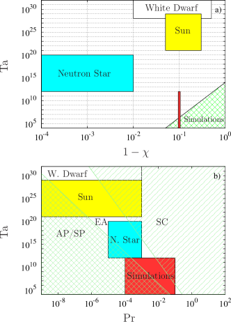
Figure 9: a) Estimates of ${\rm Ta}$ and $1-\chi$ for stellar convective oceans and parameter values of the current (red) and previous (green) numerical studies of thermal convection, which are clearly still far from stellar conditions. b) Same as a) but for ${\rm Ta}$ and $\Pr$. The estimated region of stability of the different convective instabilities SC (with stripes), EA (plain) and AP/SP (cross-hatched) is also shown.

References

- Dormy and Soward (2007) E. Dormy and A. M. Soward, eds., Mathematical Aspects of Natural Dynamos, The Fluid Mechanics of Astrophysics and Geophysics, Vol. 13 (Chapman & Hall/CRC, 2007).
- Busse (1970a) F. H. Busse, “Differential rotation in stellar convection zones,” Astrophys. J. 159, 629–639 (1970a).
- Christensen (2002) U.R. Christensen, “Zonal flow driven by strongly supercritical convection in rotating spherical shells,” J. Fluid Mech. 470, 115–133 (2002).
- Jones (2007) C. A. Jones, “Thermal and compositional convection in the outer core,” Treat. Geophys. 8, 131–185 (2007).
- Gilman (2000) P. A. Gilman, “Solar and Stellar Convection: A Perspective for Geophysical Fluid Dynamicists,” in Geophysical and Astrophysical Convection, Contributions from a workshop spinsored by the Geophysical Turbulence Program at the National Center for Atmospheric Research, October, 1995. Edited by Peter A. Fox and Robert M. Kerr. Published by Gordon and Breach Science Publishers, The Netherlands., edited by P. A. Fox and R. M. Kerr (2000) pp. 37–58.
- Roberts (1968) P. H. Roberts, “On the thermal instability of a rotating fluid sphere containing heat sources,” Phil. Trans. R. Soc. Lond. A 263, 93–117 (1968).
- Busse (1970b) F. H. Busse, “Thermal instabilities in rapidly rotating systems,” J. Fluid Mech. 44, 441–460 (1970b).
- Soward (1977) A. M. Soward, “On the finite amplitude thermal instability in a rapidly rotating fluid sphere,” Geophys. Astrophys. Fluid Dynamics 9, 19–74 (1977).
- Yano (1992) J. I. Yano, “Asymptotic theory of thermal convection in a rapidly rotating system,” J. Fluid Mech. 243, 103–131 (1992).
- Jones et al. (2000) C. A. Jones, A. M. Soward, and A. I. Mussa, “The onset of thermal convection in a rapidly rotating sphere,” J. Fluid Mech. 405, 157–179 (2000).
- Dormy et al. (2004) E. Dormy, A. M. Soward, C. A. Jones, D. Jault, and P. Cardin, “The onset of thermal convection in rotating spherical shells,” J. Fluid Mech. 501, 43–70 (2004).
- Zhang and Busse (1987) K. K. Zhang and F. H. Busse, “On the onset of convection in rotating spherical shells,” Geophys. Astrophys. Fluid Dynamics 39, 119–147 (1987).
- Zhang (1992) K. Zhang, “Spiralling columnar convection in rapidly rotating spherical fluid shells,” J. Fluid Mech. 236, 535–556 (1992).
- Massaguer (1991) J. M. Massaguer, “Stellar convection as a low Prandtl number flow,” in The Sun and Cool Stars: activity, magnetism, dynamos: Proceedings of Colloquium No. 130 of the International Astronomical Union Held in Helsinki, Finland, 17–20 July 1990, edited by I. Tuominen, D. Moss, and G. Rüdiger (Springer Berlin Heidelberg, 1991) pp. 57–61.
- Garaud et al. (2015) P. Garaud, M. Medrano, J. M. Brown, C. Mankovich, and K. Moore, “Excitation of Gravity Waves by Fingering Convection, and the Formation of Compositional Staircases in Stellar Interiors,” Astrophys. J. 808, 89 (2015).
- Zhang (1993) K. Zhang, “On equatorially trapped boundary inertial waves,” J. Fluid Mech. 248, 203–217 (1993).
- Zhang (1994) K. Zhang, “On coupling between the Poincaré equation and the heat equation,” J. Fluid Mech. 268, 211–229 (1994).
- Zhang et al. (2001) K. Zhang, P. Earnshaw, X. Liao, and Busse F.H., “On inertial waves in a rotating fluid sphere,” JFM 437, 103–119 (2001).
- Busse and Simitev (2004) F. H. Busse and R. Simitev, “Inertial convection in rotating fluid spheres,” J. Fluid Mech. 498, 23–30 (2004).
- Zhang and Liao (2004) K. Zhang and X. Liao, “A new asymptotic method for the analysis of convection in a rapidly rotating sphere,” J. Fluid Mech. 518, 319–346 (2004).
- Zhang et al. (2007) K. Zhang, X. Liao, and F.H. Busse, “Asymptotic solutions of convection in rapidly rotating non-slip spheres,” J. Fluid Mech. 578, 371–380 (2007).
- Sánchez et al. (2016) J. Sánchez, F. Garcia, and M. Net, “Radial collocation methods for the onset of convection in rotating spheres,” J. Comput. Phys. 308, 273–288 (2016).
- Zhang et al. (2017) K. Zhang, K. Lam, and D. Kong, “Asymptotic theory for torsional convection in rotating fluid spheres,” Journal of Fluid Mechanics 813 (2017), 10.1017/jfm.2017.9.
- Net et al. (2008) M. Net, F. Garcia, and J. Sánchez, “On the onset of low-Prandtl-number convection in rotating spherical shells: non-slip boundary conditions,” J. Fluid Mech. 601, 317–337 (2008).
- Garcia et al. (2008) F. Garcia, J. Sánchez, and M. Net, “Antisymmetric polar modes of thermal convection in rotating spherical fluid shells at high Taylor numbers,” Phys. Rev. Lett. 101, 194501–(1–4) (2008).
- Zhang (1995) K. Zhang, “On coupling between the Poincaré equation and the heat equation: non-slip boundary condition,” J. Fluid Mech. 284, 239–256 (1995).
- Ardes et al. (1997) M. Ardes, F. H. Busse, and J. Wicht, “Thermal convection in rotating spherical shells,” Phys. Earth Planet. Inter. 99, 55–67 (1997).
- Al-Shamali et al. (2004) F.M. Al-Shamali, M.H. Heimpel, and J.M. Aurnou, “Varying the spherical shell geometry in rotating thermal convection,” Geophys. Astrophys. Fluid Dynamics 98, 153–169 (2004).
- Busse and Or (1986) F. H. Busse and A. C. Or, “Convection in a rotating cylindrical annulus: thermal Rossby waves,” J. Fluid Mech. 166, 173–187 (1986).
- Li et al. (2010) L. Li, X. Liao, H. C. Kit, and K. Zhang, “On nonlinear multiarmed spiral waves in slowly rotating fluid systems,” PF 149 (2010).
- Chandrasekhar (1981) S. Chandrasekhar, Hydrodynamic And Hydromagnetic Stability (Dover, New York, 1981).
- Lehoucq et al. (1998) R. B. Lehoucq, D. C. Sorensen, and C. Yang, ARPACK User’s Guide: Solution of Large-Scale Eigenvalue Problems with Implicitly Restarted Arnoldi Methods (SIAM, 1998).
- Garcia et al. (2010) F. Garcia, M. Net, B. García-Archilla, and J. Sánchez, “A comparison of high-order time integrators for thermal convection in rotating spherical shells,” J. Comput. Phys. 229, 7997–8010 (2010).
- Garcia et al. (2014a) F. Garcia, E. Dormy, J. Sánchez, and M. Net, “Two computational approaches for the simulation of fluid problems in rotating spherical shells,” in Proc. of the 5th International Conference on Computational Methods - ICCM2014. Cambridge, England, Vol. 1, edited by G. R. Liu and Z. W. Guan (2014).
- Goto and van de Geijn (2008) Kazushige Goto and Robert A. van de Geijn, “Anatomy of high-performance matrix multiplication,” ACM Trans. Math. Softw. 34, 1–25 (2008).
- Ecke et al. (1992) R. E. Ecke, F. Zhong, and E. Knobloch, “Hopf bifurcation with broken reflection symmetry in rotating Rayleigh-Bénard convection,” Europhys. Lett. 19, 177–182 (1992).
- Golubitsky et al. (2000) M. Golubitsky, V. G. LeBlanc, and I. Melbourne, “Hopf bifurcation from rotating waves and patterns in physical space,” J. Nonlinear Sci. 10, 69–101 (2000).
- Sánchez et al. (2013) J. Sánchez, F. Garcia, and M. Net, “Computation of azimuthal waves and their stability in thermal convection in rotating spherical shells with application to the study of a double-Hopf bifurcation,” Phys. Rev. E 87, 033014/ 1–11 (2013).
- Roberts (1965) P. H. Roberts, “On the thermal instability of a highly rotating fluid sphere,” Astrophys. J. 141, 240–250 (1965).
- Spiegel and Veronis (1960) E. A. Spiegel and G. Veronis, “On the boussinesq approximation for a compressible fluid,” Astrophys. J. 131, 442–447 (1960).
- Chen and Glatzmaier (2005) Q. Chen and G.A. Glatzmaier, “Large eddy simulations of two-dimensional turbulent convection in a density-stratified fluid,” Geophys. Astrophys. Fluid Dynamics 99, 355–375 (2005).
- Jones et al. (2009) C. A. Jones, K. M. Kuzayan, and R. H. Mitchell, “Linear theory of compressible convection in rapidly rotating spherical shells, using the anelastic approximation,” J. Fluid Mech. 634, 291–319 (2009).
- Calkins et al. (2015) Michael A. Calkins, Keith Julien, and Philippe Marti, “The breakdown of the anelastic approximation in rotating compressible convection: implications for astrophysical systems,” Proceedings of the Royal Society of London A: Mathematical, Physical and Engineering Sciences 471 (2015).
- Wood and Bushby (2016) T. S. Wood and P. J. Bushby, “Oscillatory convection and limitations of the Boussinesq approximation,” J. Fluid Mech. 803, 502–515 (2016).
- Brummell and Toomre (1995) N. Brummell and J. Toomre, “Modelling astrophysical turbulent convection,” in Astronomical Data Analysis Software and Systems IV, ASP Conference Series, Vol. 77, edited by R. A. Shaw, H. E. Payne, and J. J. E. Hayes (1995) pp. 15–24.
- Brandenburg et al. (2000) A. Brandenburg, A. Nordlund, and R. F. Stein, “Astrophysical convection and dynamos,” in Geophysical and Astrophysical Convection, Contributions from a workshop spinsored by the Geophysical Turbulence Program at the National Center for Atmospheric Research, October, 1995. Edited by Peter A. Fox and Robert M. Kerr. Published by Gordon and Breach Science Publishers, The Netherlands, 2000, p. 85-105, edited by P. A. Fox and R. M. Kerr (2000) pp. 85–105.
- Landeau and Aubert (2011) M. Landeau and J. Aubert, “Equatorially asymmetric convection inducing a hemispherical magnetic field in rotating spheres and implications for the past martian dynamo,” Physics of the Earth and Planetary Interiors 185, 61 – 73 (2011).
- Garcia et al. (2014b) F. Garcia, L. Bonaventura, M. Net, and J. Sánchez, “Exponential versus imex high-order time integrators for thermal convection in rotating spherical shells,” J. Comput. Phys. 264, 41–54 (2014b).
- Nandkumar and Pethick (1984) R. Nandkumar and C. J. Pethick, “Transport coefficients of dense matter in the liquid metal regime,” Mon. Not. R. astr. Soc. 209, 511–524 (1984).
- Isern et al. (2017) J. Isern, E. García-Berro, B. Külebi, and P. Lorén-Aguilar, “A Common Origin of Magnetism from Planets to White Dwarfs,” Astrophys. J. Lett. 836, L28 (2017).
- Yakovlev and Urpin (1980) D. G. Yakovlev and V. A. Urpin, “Thermal and Electrical Conductivity in White Dwarfs and Neutron Stars,” Soviet Ast. 24, 303 (1980).
- Watts (2012) A. L. Watts, “Thermonuclear Burst Oscillations,” Ann. Rev. Astron. Astrophys. 50, 609–640 (2012).
- Bagenal et al. (2004) F. Bagenal, T. E. Dowling, and W. McKinnon, Jupiter: The planet, satellites and magnetosphere (Cambridge University press, Cambridge, 2004).
- Showman et al. (2011) A. P. Showman, Y. Kaspi, and G. R. Flierl, “Scaling laws for convection and jet speeds in the giant planets,” ICARUS 211, 1258–1273 (2011).
- Herwig et al. (2006) F. Herwig, B. Freytag, R. M. Hueckstaedt, and F. X. Timmes, “Hydrodynamic Simulations of He Shell Flash Convection,” Astrophys. J. 642, 1057–1074 (2006), astro-ph/0601164 .
- Meakin and Arnett (2007) C. A. Meakin and D. Arnett, “Turbulent Convection in Stellar Interiors. I. Hydrodynamic Simulation,” Astrophys. J. 667, 448–475 (2007), astro-ph/0611315 .
- Mocák et al. (2009) M. Mocák, E. Müller, A. Weiss, and K. Kifonidis, “The core helium flash revisited. II. Two and three-dimensional hydrodynamic simulations,” Astronomy & Astrophysics 501, 659–677 (2009), arXiv:0811.4083 .
- Kippenhahn et al. (2013) Rudolf Kippenhahn, Alfred Weigert, and Achim Weiss, Stellar Structure and Evolution; 2nd ed., Astronomy and Astrophysics Library (Springer, Berlin, 2013).
- Shankar et al. (1992) A. Shankar, D. Arnett, and B. A. Fryxell, “Thermonuclear runaways in nova outbursts,” Astrophysical Journal Letters 394, L13–L15 (1992).
- Glasner and Livne (1995) S. A. Glasner and E. Livne, “Convective hydrogen burning down a nova outburst,” Astrophysical Journal Letters 445, L149–L151 (1995).
- Kercek et al. (1999) A. Kercek, W. Hillebrandt, and J. W. Truran, “Three-dimensional simulations of classical novae,” Astronomy & Astrophysics 345, 831–840 (1999), astro-ph/9811259 .
- Starrfield et al. (2016) S. Starrfield, C. Iliadis, and W. R. Hix, “The Thermonuclear Runaway and the Classical Nova Outburst,” Publications of the Astronomical Society of the Pacific 128, 051001 (2016), arXiv:1605.04294 [astro-ph.SR] .
- Miesch (2000) M.S. Miesch, “The coupling of solar convection and rotation,” Solar Physics 192, 59–89 (2000).
- Paternò (2010) L. Paternò, “The solar differential rotation: a historical view,” Astrophysics and Space Science 328, 269–277 (2010).
- Brun et al. (2015) A. S. Brun, R. A. García, G. Houdek, D. Nandy, and M. Pinsonneault, “The Solar-Stellar Connection,” Space Sci. Rev. 196, 303–356 (2015).
- Hanasoge et al. (2016) S. Hanasoge, L. Gizon, and K. R. Sreenivasan, “Seismic sounding of convection in the sun,” Ann. Rev. Fluid Mech. 48, 191–217 (2016).
- Glatzmaier (1984) G.A. Glatzmaier, “Numerical simulations of stellar convective dynamos. I. The model and method,” J. Comput. Phys. 55, 461–484 (1984).
- Miesch et al. (2000) M. S. Miesch, J. R. Elliot, J. Toomre, T. L. Clune, G. A. Glatzmaier, and P. A. Gilman, “Three-dimensional spherical simulation of solar convection. I. Diferential rotation and pattern evolution achieved with laminar and turbulent states,” The Astrophysical Journal 532, 593–615 (2000).
- Miesch et al. (2006) M. S. Miesch, A. S. Brun, and J. Toomre, “Solar differential rotation influenced by latitudinal entropy variations in the tachocline,” The Astrophysical Journal 641, 618 (2006).
- Ogurtsov et al. (2002) M.G. Ogurtsov, Yu.A. Nagovitsyn, G.E. Kocharov, and H. Jungner, “Long-period cycles of the sun’s activity recorded in direct solar data and proxies,” Solar Physics 211, 371–394 (2002).
- Kern et al. (2012) A.K. Kern, M. Harzhauser, W.E. Piller, O. Mandic, and A. Soliman, “Strong evidence for the influence of solar cycles on a late miocene lake system revealed by biotic and abiotic proxies,” Palaeogeography, Palaeoclimatology, Palaeoecology 329, 124 – 136 (2012).
- Xapsos and Burke (2009) M. A. Xapsos and E. A. Burke, “Evidence of 6 000-year periodicity in reconstructed sunspot numbers,” Solar Physics 257, 363–369 (2009).
- Sánchez-Sesma (2016) J. Sánchez-Sesma, “Evidence of cosmic recurrent and lagged millennia-scale patterns and consequent forecasts: multi-scale responses of solar activity (sa) to planetary gravitational forcing (pgf),” Earth System Dynamics 7, 583–595 (2016).
- Parker (1955) E. N. Parker, “Hydromagnetic Dynamo Models,” Astrophys. J. 122, 293 (1955).
- Choudhuri et al. (2007) A. R. Choudhuri, P. Chatterjee, and J. Jiang, “Predicting solar cycle 24 with a solar dynamo model,” Phys. Rev. Lett. 98, 131103 (2007).
- Strugarek et al. (2017) A. Strugarek, P. Beaudoin, P. Charbonneau, A. S. Brun, and J.-D. do Nascimento, “Reconciling solar and stellar magnetic cycles with nonlinear dynamo simulations,” Science 357, 185–187 (2017).
- Usoskin (2017) I. G. Usoskin, “A history of solar activity over millennia,” Living Reviews in Solar Physics 14, 3 (2017).
- Schatzman (1958) E. L. Schatzman, Amsterdam, North-Holland Pub. Co.; New York, Interscience Publishers, 1958. (1958).
- Fontaine and van Horn (1976) G. Fontaine and H. M. van Horn, “Convective white-dwarf envelope model grids for H-, He-, and C-rich compositions,” Astrophysical Journal Supplement Series 31, 467–487 (1976).
- Tremblay et al. (2013) P.-E. Tremblay, H.-G. Ludwig, M. Steffen, and B. Freytag, “Pure-hydrogen 3D model atmospheres of cool white dwarfs,” Astronomy & Astrophysics 552, A13 (2013), arXiv:1302.2013 [astro-ph.SR] .
- Kawaler (2004) S. D. Kawaler, “White Dwarf Rotation: Observations and Theory (Invited Review),” in Stellar Rotation, IAU Symposium, Vol. 215, edited by A. Maeder and P. Eenens (2004) p. 561.
- Strohmayer and Bildsten (2006) T. Strohmayer and L. Bildsten, “New views of thermonuclear bursts,” in Compact stellar X-ray sources (2006) pp. 113–156.
- Malone et al. (2011) C. M. Malone, A. Nonaka, A. S. Almgren, J. B. Bell, and M. Zingale, “Multidimensional Modeling of Type I X-ray Bursts. I. Two-dimensional Convection Prior to the Outburst of a Pure 4He Accretor,” ApJ 728, 118 (2011), arXiv:1012.0609 [astro-ph.HE] .
- Malone et al. (2014) C. M. Malone, M. Zingale, A. Nonaka, A. S. Almgren, and J. B. Bell, “Multidimensional Modeling of Type I X-Ray Bursts. II. Two-dimensional Convection in a Mixed H/He Accretor,” ApJ 788, 115 (2014), arXiv:1404.6286 [astro-ph.HE] .
- Keek and Heger (2017) L. Keek and A. Heger, “Thermonuclear Bursts with Short Recurrence Times from Neutron Stars Explained by Opacity-driven Convection,” ApJ 842, 113 (2017), arXiv:1706.00786 [astro-ph.HE] .
- Hook and Hall (1991) J.R. Hook and H.E. Hall, Solid state physics, The Manchester physics series (Wiley, 1991).
- Spitkovsky et al. (2002) A. Spitkovsky, Y. Levin, and G. Ushomirsky, “Propagation of Thermonuclear Flames on Rapidly Rotating Neutron Stars: Extreme Weather during Type I X-Ray Bursts,” Astrophys. J. 566, 1018–1038 (2002), astro-ph/0108074 .
- Cavecchi et al. (2013) Y. Cavecchi, A. L. Watts, J. Braithwaite, and Y. Levin, “Flame propagation on the surfaces of rapidly rotating neutron stars during Type I X-ray bursts,” MNRAS 434, 3526–3541 (2013), arXiv:1212.2872 [astro-ph.HE] .
- Cavecchi et al. (2015) Y. Cavecchi, A. L. Watts, Y. Levin, and J. Braithwaite, “Rotational effects in thermonuclear type I bursts: equatorial crossing and directionality of flame spreading,” MNRAS 448, 445–455 (2015), arXiv:1411.2284 [astro-ph.HE] .
- Cavecchi et al. (2016) Y. Cavecchi, Y. Levin, A. L. Watts, and J. Braithwaite, “Fast and slow magnetic deflagration fronts in type I X-ray bursts,” MNRAS 459, 1259–1275 (2016), arXiv:1509.02497 [astro-ph.HE] .
- Mahmoodifar and Strohmayer (2016) S. Mahmoodifar and T. Strohmayer, “X-Ray Burst Oscillations: From Flame Spreading to the Cooling Wake,” Astrophys. J. 818, 93 (2016), arXiv:1510.05005 [astro-ph.HE] .
- Heyl (2004) J. S. Heyl, “r-Modes on Rapidly Rotating, Relativistic Stars. I. Do Type I Bursts Excite Modes in the Neutron Star Ocean?” Astrophys. J. 600, 939–945 (2004), astro-ph/0108450 .
- Piro and Bildsten (2005) A. L. Piro and L. Bildsten, “Surface Modes on Bursting Neutron Stars and X-Ray Burst Oscillations,” Astrophys. J. 629, 438–450 (2005), astro-ph/0502546 .

References

- Zhang (1992) K. Zhang, “Spiralling columnar convection in rapidly rotating spherical fluid shells,” J. Fluid Mech. 236, 535–556 (1992).
- Nandkumar and Pethick (1984) R. Nandkumar and C. J. Pethick, “Transport coefficients of dense matter in the liquid metal regime,” Mon. Not. R. astr. Soc. 209, 511–524 (1984).
- Yakovlev and Urpin (1980) D. G. Yakovlev and V. A. Urpin, “Thermal and Electrical Conductivity in White Dwarfs and Neutron Stars,” Soviet Ast. 24, 303 (1980).
- Watts (2012) A. L. Watts, “Thermonuclear Burst Oscillations,” Ann. Rev. Astron. Astrophys. 50, 609–640 (2012).