Iterative Sparse Asymptotic Minimum Variance Based Approaches for Array Processing

Abstract

This paper presents a series of user parameter-free iterative Sparse Asymptotic Minimum Variance (SAMV) approaches for array processing applications based on the asymptotically minimum variance (AMV) criterion. With the assumption of abundant snapshots in the direction-of-arrival (DOA) estimation problem, the signal powers and noise variance are jointly estimated by the proposed iterative AMV approach, which is later proved to coincide with the Maximum Likelihood (ML) estimator. We then propose a series of power-based iterative SAMV approaches, which are robust against insufficient snapshots, coherent sources and arbitrary array geometries. Moreover, to overcome the direction grid limitation on the estimation accuracy, the SAMV-Stochastic ML (SAMV-SML) approaches are derived by explicitly minimizing a closed form stochastic ML cost function with respect to one scalar parameter, eliminating the need of any additional grid refinement techniques. To assist the performance evaluation, approximate solutions to the SAMV approaches are also provided at high signal-to-noise ratio (SNR) and low SNR, respectively. Finally, numerical examples are generated to compare the performance of the proposed approaches with existing approaches.

Index terms: Array Processing, AMV estimator, Direction-Of-Arrival (DOA) estimation, Sparse parameter estimation, Covariance matrix, Iterative methods, Vectors, Arrays, Maximum likelihood estimation, Signal to noise ratio, SAMV approach.

Preprint version PDF available on arXiv. Official version: Abeida Habti, Qilin Zhang, Jian Li, and Nadjim Merabtine. “Iterative sparse asymptotic minimum variance based approaches for array processing.” IEEE Transactions on Signal Processing 61, no. 4 (2013): 933-944.
Matlab implementation codes available online, https://qilin-zhang.github.io/publications/

 

I Introduction

Sparse signal representation has attracted a lot of attention in recent years and it has been successfully used for solving inverse problems in various applications such as channel equalization (e.g., [7, 8, 9, 10]), source localization (e.g., [15, 16, 35, 34]) and radar imaging (e.g., [11, 12, 13, 14]). In its basic form, it attempts to find the sparsest signal ${\bf x}$ satisfying the constrain ${\bf y}={\bf A}{\bf x}$ or ${\bf y}={\bf A}{\bf x}+{\bf e}$ where ${\bf A}\in\mathbb{C}^{M\times K}$ is an overcomplete basis (i.e., $K>M$), ${\bf y}$ is the observation data, and ${\bf e}$ is the noise term. Theoretically, this problem is underdetermined and has multiple solutions. However, the additional constraint that ${\bf x}$ should be sparse allows one to eliminate the ill-posedness (e.g., [1, 2]). In recent years, a number of practical algorithms such as $\ell_{1}$ norm minimization (e.g., [3, 4]) and focal underdetermined system solution (FOCUSS) (e.g., [5, 6]) have been proposed to approximate the sparse solution.

Conventional subspace-based source localization algorithms such as multiple signal classification (MUSIC) and estimation of signal parameters via a rotational invariance technique (ESPRIT) [17, 18] are only applicable when $M>K$, and they require sufficient snapshots and high signal-to-noise ratio (SNR) to achieve high spatial resolution. However, it is often unpractical to collect a large number of snapshots, especially in fast time-varying environment, which deteriorates the construction accuracy of the subspaces and degrades the localization performance. In addition, even with appropriate array calibration, subspace-based methods are incapable of handling the source coherence due to their sensitivity to subspace orthogonality (e.g., [17, 19]).

Recently, a user parameter-free non-parametric algorithm, the iterative adaptive approach (IAA), has been proposed in [16] and employed in various applications (e.g., [12, 13]). It is demonstrated in these works that the least square fitting-based IAA algorithm provides accurate DOA and signal power estimates, and it is insensitive to practical impairments such as few (even one) snapshots, arbitrary array geometries and coherent sources. However, the iterative steps are based on the IAA covariance matrix ${\bf R}={\bf A}{{\rm Diag}({\bf p})}{\bf A}^{H}$, which could be singular in the noise-free scenarios when only a few components of the power vector ${\bf p}$ are non-zero. In addition, a regularized version of the IAA algorithm (IAA-R) is later proposed in [13] for single-snapshot and nonuniform white noise cases. Stoica et al. have recently proposed a user parameter-free SParse Iterative Covariance-based Estimation (SPICE) approach in [20, 21] based on minimizing a covariance matrix fitting criterion. However, the SPICE approach proposed in [20] for the multiple-snapshot case depends on the inverse of the sample covariance matrix, which exists only if the number of snapshot $N$ is larger than $M$ [31]. Therefore, this approach also suffers from insufficient snapshots when $N<M$. We note that the source localization performance of the power-based algorithms is mostly limited by the fineness of the direction grid [15].

In this paper, we propose a series of iterative Sparse Asymptotic Minimum Variance (SAMV) approaches based on the asymptotically minimum variance (AMV) approach (also called asymptotically best consistent (ABC) estimators in [23]), which is initially proposed for DOA estimation in [28, 27]. After presenting the sparse signal representation data model for the DOA estimation problem in Section II, we first propose an iterative AMV approach in Section III, which is later proven to be identical to the stochastic Maximum Likelihood (ML) estimator. Based on this approach, we then propose the user parameter-free iterative SAMV approaches that can handle arbitrary number of snapshots ($N<M$ or $N>M$), and only a few non-zero components in the power estimates vector ${\bf p}$ in Section IV. In addition, A series of SAMV-Stochastic ML (SAMV-SML) approaches are proposed in Section V to alleviate the direction grid limitation and enhance the performance of the power-based SAMV approaches. In Section VI, we derive approximate expressions for the SAMV powers-iteration formulas at both high and low SNR. In Section VII, numerical examples are generated to compare the performances of the proposed approaches with existing approaches. Finally, conclusions are given in Section VIII.

The following notations are used throughout the paper. Matrices and vectors are represented by bold upper case and bold lower case characters, respectively. Vectors are by default in column orientation, while $T$, $H$, and $*$ stand for transpose, conjugate transpose, and conjugate, respectively. ${\rm E}(\cdot)$, ${\rm Tr}(\cdot)$ and $\det(\cdot)$ are the expectation, trace and determinant operators, respectively. ${\rm vec}(\cdot)$ is the “vectorization” operator that turns a matrix into a vector by stacking all columns on top of one another, $\otimes$ denotes the Kronecker product, ${\bf I}$ is the identity matrix of appropriate dimension, and ${\bf e}_{m}$ denotes the $m$th column of ${\bf I}$.

II Problem Formation and Data Model

Consider an array of $M$ omnidirectional sensors receiving $K$ narrowband signals impinging from the sources located at $\boldsymbol{\theta}\stackrel{{\scriptstyle{\rm def}}}{{=}}(\theta_{1},\ldots,\theta_{K})$ where $\theta_{k}$ denotes the location parameter of the $k$th signal, $k=1,\ldots,K$. The $M\times 1$ array snapshot vectors can be modeled as (see e.g., [16, 20])

$${\bf y}(n)={\bf A}{\bf x}(n)+{\bf e}(n),\;n=1,\ldots,N,$$ (1)

where ${\bf A}\stackrel{{\scriptstyle{\rm def}}}{{=}}[{\bf a}(\theta_{1}),\ldots,{\bf a}(\theta_{K})]$ is the steering matrix with each column being a steering vector ${\bf a}_{k}\stackrel{{\scriptstyle{\rm def}}}{{=}}{\bf a}(\theta_{k})$, a known function of $\theta_{k}$. The vector ${\bf x}(n)\stackrel{{\scriptstyle{\rm def}}}{{=}}[{\bf x}_{1}(n),\ldots,{\bf x}_{K}(n)]^{T}$ contains the source waveforms, and ${\bf e}(n)$ is the noise term. Assume that ${\rm E}\left({\bf e}(n){\bf e}^{H}(\bar{n})\right)=\sigma{\bf I}_{M}\delta_{n,\bar{n}}$, where $\delta_{n,\bar{n}}$ is the Dirac delta and it equals to $1$ only if $n=\bar{n}$ and $0$ otherwise. We also assume first that ${\bf e}(n)$ and ${\bf x}(n)$ are independent, and that ${\rm E}\left({\bf x}(n){\bf x}^{H}(\bar{n})\right)={\bf P}\delta_{n,\bar{n}}$, where ${\bf P}\stackrel{{\scriptstyle{\rm def}}}{{=}}{\rm Diag}({p_{1},\ldots,p_{K}})$. Let ${\bf p}$ be a vector containing the unknown signal powers and noise variance, ${\bf p}\stackrel{{\scriptstyle{\rm def}}}{{=}}[p_{1},\ldots,p_{K},\sigma]^{T}$.

The covariance matrix of ${\bf y}(n)$ that conveys information about $\boldsymbol{\bf p}$ is given by

$${\bf R}\stackrel{{\scriptstyle{\rm def}}}{{=}}{\bf A}{\bf P}{\bf A}^{H}+\sigma{\bf I}.$$

This covariance matrix is traditionally estimated by the sample covariance matrix ${\bf R}_{N}\stackrel{{\scriptstyle{\rm def}}}{{=}}{\bf Y}{\bf Y}^{H}/N$ where ${\bf Y}\stackrel{{\scriptstyle{\rm def}}}{{=}}[{\bf y}(1),\ldots,{\bf y}(N)]$. After applying the vectorization operator to the matrix ${\bf R}$, the obtained vector ${\bf r}(\boldsymbol{\bf p})\stackrel{{\scriptstyle{\rm def}}}{{=}}{\rm vec}({\bf R})$ is linearly related to the unknown parameter $\boldsymbol{\bf p}$ as

$${\bf r}(\boldsymbol{\bf p})\stackrel{{\scriptstyle{\rm def}}}{{=}}{\rm vec}({\bf R})={\bf S}\boldsymbol{\bf p},$$ (2)

where ${\bf S}\stackrel{{\scriptstyle{\rm def}}}{{=}}[{\bf S}_{1},\bar{\bf a}_{K+1}]$, ${\bf S}_{1}=[\bar{\bf a}_{1},\ldots,\bar{\bf a}_{K}]$, $\bar{\bf a}_{k}\stackrel{{\scriptstyle{\rm def}}}{{=}}{\bf a}^{*}_{k}\otimes{\bf a}_{k}$, $k=1,\ldots K$, and $\bar{\bf a}_{K+1}\stackrel{{\scriptstyle{\rm def}}}{{=}}{\rm vec}({\bf I})$.

We note that the Gaussian circular asymptotic covariance matrix ${\bf r}_{N}\stackrel{{\scriptstyle{\rm def}}}{{=}}{\rm vec}({\bf R}_{N})$ is given by [29, Appendix B], [28]

$${\bf C}_{r}={\bf R}^{*}\otimes{\bf R}.$$

The number of sources, $K$, is usually unknown. The power-based algorithms, such as the proposed SAMV approaches, use a predefined scanning direction grid $\{\theta_{k}\}_{k=1}^{K}$ to cover the entire region-of-interest $\bf\Omega$, and every point in this grid is considered as a potential source whose power is to be estimated. Consequently, $K$ is the number of points in the grid and it is usually much larger than the actual number of sources present, and only a few components of $\boldsymbol{\bf p}$ will be non-zero. This is the main reason why sparse algorithms can be used in array processing applications [20, 21].

To estimate the parameter $\boldsymbol{\bf p}$ from the statistic ${\bf r}_{N}$, we develop a series of iterative SAMV approaches based on the AMV approach introduced by Porat and Fridelander in [22], Stoica et al. in [23] with their asymptotically best consistent (ABC) estimator, and Delmas and Abeida in [28, 27].

III The asymptotically minimum variance approach

In this section, we develop a recursive approach to estimate the signal powers and noise variance (i.e., $\boldsymbol{\bf p}$) based on the AMV criterion using the statistic ${\bf r}_{N}$. We assume that $\boldsymbol{\bf p}$ is identifiable from ${\bf r}(\boldsymbol{\bf p})$. Exploiting the similarities to the works in [28, 27], it is straightforward to prove that the covariance matrix ${\bf Cov}^{\rm Alg}_{\boldsymbol{p}}$ of an arbitrary consistent estimator of $\boldsymbol{p}$ based on the second-order statistic ${\bf r}_{N}$ is bounded below by the following real symmetric positive definite matrix:

$${\bf Cov}^{\rm Alg}_{\boldsymbol{p}}\geq[{\bf S}^{H}_{d}{\bf C}^{-1}_{r}{\bf S}_{d}]^{-1},$$

where ${\bf S}_{d}\stackrel{{\scriptstyle{\rm def}}}{{=}}{\rm d}{\bf r}(\boldsymbol{p})/{\rm d}\boldsymbol{p}$. In addition, this lower bound is attained by the covariance matrix of the asymptotic distribution of $\hat{\bf p}$ obtained by minimizing the following AMV criterion:

$$\hat{\boldsymbol{p}}=\arg\min_{\boldsymbol{p}}f(\boldsymbol{p}),$$

where

$$f(\boldsymbol{p})\stackrel{{\scriptstyle{\rm def}}}{{=}}[{\bf r}_{N}-{\bf r}(\boldsymbol{p})]^{H}{\bf C}_{r}^{-1}[{\bf r}_{N}-{\bf r}(\boldsymbol{p})].$$ (3)

From (3) and using (2), the estimate of $\boldsymbol{\bf p}$ is given by the following results proved in Appendix A:

Result 1.

The $\{\hat{p}_{k}\}_{k=1}^{K}$ and $\hat{\sigma}$ that minimize (3) can be computed iteratively. Assume $\hat{p}^{(i)}_{k}$ and $\hat{\sigma}^{(i)}$ have been obtained in the $i$th iteration, they can be updated at the $(i+1)$th iteration as:

$$\hat{p}^{(i+1)}_{k} = \frac{{\bf a}^{H}_{k}{\bf R}^{-1{(i)}}{\bf R}_{N}{\bf R}^{-1{(i)}}{\bf a}_{k}}{({\bf a}^{H}_{k}{\bf R}^{-1{(i)}}{\bf a}_{k})^{2}}+\hat{p}^{(i)}_{k}-\frac{1}{{\bf a}^{H}_{k}{\bf R}^{-1{(i)}}{\bf a}_{k}},\;\;k=1\ldots,K,$$ (4)

$$\hat{\sigma}^{(i+1)} = \left({\rm Tr}({\bf R}^{-2^{(i)}}{\bf R}_{N})+\hat{\sigma}^{(i)}{\rm Tr}({\bf R}^{-2^{(i)}})-{\rm Tr}({\bf R}^{-1^{(i)}})\right)/{{\rm Tr}{({\bf R}^{-2^{(i)}})}},$$ (5)

where the estimate of ${\bf R}$ at the $i$th iteration is given by ${\bf R}^{(i)}={\bf A}{\bf P}^{(i)}{\bf A}^{H}+\hat{\sigma}^{(i)}{\bf I}$ with ${\bf P}^{(i)}={\rm Diag}(\hat{p}^{(i)}_{1},\ldots,\hat{p}^{(i)}_{K}).$

Assume that ${\bf x}(n)$ and ${\bf e}(n)$ are both circularly Gaussian distributed, ${\bf y}(n)$ also has a circular Gaussian distribution with zero-mean and covariance matrix ${\bf R}$. The stochastic negative log-likelihood function of $\{{\bf y}(n)\}_{n=1}^{N}$ can be expressed as (see, e.g., [26, 16])

$$L(\boldsymbol{\bf p})=\ln(\det({\bf R}))+{\rm Tr}({\bf R}^{-1}{\bf R}_{N}).$$ (6)

In lieu of the cost function (3) that depends linearly on $\boldsymbol{\bf p}$ (see (2)), this ML cost-function (6) depends non-linearly on the signal powers and noise variance embedded in ${\bf R}$. Despite this difficulty and reminiscent of [16], we prove in Appendix B that the following result holds:

Result 2.

The estimates given by (4) and (5) are identical to the ML estimates.

Consequently, there always exists approaches that gives the same performance as the ML estimator which is asymptotically efficient. Returning to the Result 1, first we notice that the expression given by (4) remains valid regardless of $K>M$ or $K<M$. In the scenario where $K>M$, we observe from numerical calculations that the $\hat{p}_{k}$ and $\hat{\sigma}$ given by (4) and (5) may be negative; therefore, the nonnegativity of the power estimates can be enforced at each iteration by forcing the negative estimates to zero as [16, Eq. (30)],

$$\hat{p}^{(i+1)}_{k} = \max\left(0,\frac{{\bf a}^{H}_{k}{\bf R}^{-1{(i)}}{\bf R}_{N}{\bf R}^{-1{(i)}}{\bf a}_{k}}{({\bf a}^{H}_{k}{\bf R}^{-1{(i)}}{\bf a}_{k})^{2}}+\hat{p}^{(i)}_{k}-\frac{1}{{\bf a}^{H}_{k}{\bf R}^{-1{(i)}}{\bf a}_{k}}\right),\;\;k=1\ldots,K,$$ (7)

$$\hat{\sigma}^{(i+1)} = \max\left(0,\left({\rm Tr}({\bf R}^{-2^{(i)}}{\bf R}_{N})+\hat{\sigma}^{(i)}{\rm Tr}({\bf R}^{-2^{(i)}})-{\rm Tr}({\bf R}^{-1^{(i)}})\right)/{{\rm Tr}{({\bf R}^{-2^{(i)}})}}\right).$$

The above updating formulas of $\hat{p}_{k}$ and $\hat{\sigma}$ at $(i+1)$th iteration require knowledge of ${\bf R}$, $\hat{p}_{k}$ and $\hat{\sigma}$ at the $i$th iteration, hence this algorithm must be implemented iteratively. The initialization of $\hat{p}_{k}$ can be done with the periodogram (PER) power estimates (see, e.g., [30])

$$\hat{p}^{(0)}_{k,{\rm PER}}=\frac{{\bf a}^{H}_{k}{\bf R}_{N}{\bf a}_{k}}{\|{\bf a}_{k}\|^{4}}.$$ (8)

The noise variance estimator $\hat{\sigma}$ can be initialized as, for instance,

$$\hat{\sigma}=\frac{1}{MN}\sum_{n=1}^{N}\|{\bf y}(n)\|^{2}.$$ (9)

Remark 1.

In the classical scenario where there are more sensors than sources (i.e., $K\leq M$), closed form approximate ML estimates of a single source power and noise variance are derived in [25] and [24] assuming uniform white noise and nonuniform white noise, respectively. However, these approximate expressions are derived at high and low SNR regimes separately, compared to the unified expressions (4) and (5) regardless of SNR or number of sources.

Remark 2.

Result 1 can be extended easily to the nonuniform white Gaussian noise case where the covariance matrix is given by

$${\rm E}\left({\bf e}(n){\bf e}^{H}(n)\right)={\rm Diag}(\sigma_{1},\ldots,\sigma_{M})\stackrel{{\scriptstyle{\rm def}}}{{=}}\sum_{m=1}^{M}\sigma_{m}{\bf a}_{K+m}{\bf a}^{T}_{K+m},$$ (10)

where ${\bf a}_{K+m}\stackrel{{\scriptstyle{\rm def}}}{{=}}{\bf e}_{m}$, $m=1,\ldots,M$, denote the canonical vectors. Under these assumptions and from Result 1, the estimates of ${\bf p}$ at $(i+1)$th iteration are given by

$$\hat{p}^{(i+1)}_{k}=\frac{{\bf a}^{H}_{k}{\bf R}^{-1{(i)}}{\bf R}_{N}{\bf R}^{-1{(i)}}{\bf a}_{k}}{({\bf a}^{H}_{k}{\bf R}^{-1{(i)}}{\bf a}_{k})^{2}}+\hat{p}^{(i)}_{k}-\frac{1}{{\bf a}^{H}_{k}{\bf R}^{-1{(i)}}{\bf a}_{k}},\;k=1\ldots,K+M,$$ (11)

where ${\bf R}^{{(i)}}={\bf A}{\bf P}^{{(i)}}{\bf A}^{H}+\sum_{m=1}^{M}\hat{\sigma}^{{(i)}}_{m}{\bf a}_{K+m}{\bf a}^{T}_{K+m}$, ${\bf P}^{(i)}={\rm Diag}(\hat{p}^{(i)}_{1},\ldots,\hat{p}^{(i)}_{K})$ and $\hat{\sigma}^{{(i)}}_{m}=\hat{p}^{{(i)}}_{K+m}$, $m=1,\ldots,M$.

As mentioned before, the $\hat{p}_{k}$ may be negative when $K>M$, therefore, the power estimates can be iterated similar to (7) by forcing the negative values to zero.

IV The sparse asymptotic minimum variance Approaches

In this section, we propose the iterative SAMV approaches to estimate $\boldsymbol{\bf p}$ even when $K$ exceeds the number of sources $K$(i.e., when the steering matrix ${\bf A}$ can be viewed as an overcomplete basis for ${\bf y}(n)$) and only a few non-zero components are present in ${\bf p}$. This is the common case encountered in many spectral analysis applications, where only the estimation of ${\bf p}$ is deemed relevant (e.g., [20, 21]).

As mentioned in Result 2, the estimates given by (4) and (5) may give irrational negative values due to the presence of the non-zero terms $p_{k}-1/({\bf a}^{H}_{k}{\bf R}^{-1}{\bf a}_{k})$ and $\sigma-{\rm Tr}({\bf R}^{-1})/{\rm Tr}({\bf R}^{-2})$. To resolve this difficulty, we assume that $p_{k}=1/({\bf a}^{H}_{k}{\bf R}^{-1}{\bf a}_{k})$ and $\sigma={\rm Tr}({\bf R}^{-1})/{\rm Tr}({\bf R}^{-2})$, and propose the following SAMV approaches based on Result 1:

SAMV-0 approach:
The estimates of $p_{k}$ and ${\sigma}$ are updated at $(i+1)$th iteration as:

$$\hat{p}^{(i+1)}_{k} = \hat{p}^{2(i)}_{k}({\bf a}^{H}_{k}{\bf R}^{-1(i)}{\bf R}_{N}{\bf R}^{-1(i)}{\bf a}_{k}),\;k=1,\ldots,K,$$ (12)

$$\noindent\hat{\sigma}^{(i+1)} = \frac{{\rm Tr}({\bf R}^{-2(i)}{\bf R}_{N})}{{\rm Tr}({\bf R}^{-2(i)})}.$$ (13)

SAMV-1 approach:
The estimates of $p_{k}$ and ${\sigma}$ are updated at $(i+1)$th iteration as:

$$\hat{p}^{(i+1)}_{k} = \frac{{\bf a}^{H}_{k}{\bf R}^{-1(i)}{\bf R}_{N}{\bf R}^{-1(i)}{\bf a}_{k}}{({\bf a}^{H}_{k}{\bf R}^{-1(i)}{\bf a}_{k})^{2}},\;k=1,\ldots,K,$$ (14)

$$\hat{\sigma}^{(i+1)} = \frac{{\rm Tr}({\bf R}^{-2(i)}{\bf R}_{N})}{{\rm Tr}({\bf R}^{-2(i)})}.$$ (15)

SAMV-2 approach:
The estimates of $p_{k}$ and ${\sigma}$ are updated at $(i+1)$th iteration as:

$$\hat{p}^{(i+1)}_{k} = \hat{p}^{(i)}_{k}\frac{{\bf a}^{H}_{k}{\bf R}^{-1(i)}{\bf R}_{N}{\bf R}^{-1(i)}{\bf a}_{k}}{{\bf a}^{H}_{k}{\bf R}^{-1(i)}{\bf a}_{k}},\;k=1,\ldots,K,$$ (16)

$$\hat{\sigma}^{(i+1)} = \frac{{\rm Tr}({\bf R}^{-2(i)}{\bf R}_{N})}{{\rm Tr}({\bf R}^{-2(i)})}.$$

In the case of nonuniform white Gaussian noise with covariance matrix given in Remark 2, the SAMV noise powers estimates can be updated alternatively as

$$\hat{\sigma}^{(i+1)}_{m}=\frac{{\bf e}^{H}_{m}{\bf R}^{-1{(i)}}{\bf R}_{N}{\bf R}^{-1{(i)}}{\bf e}_{m}}{({\bf e}^{H}_{m}{\bf R}^{-1{(i)}}{\bf e}_{m})^{2}},\;\;m=1\ldots,M,$$ (17)

where ${\bf R}^{{(i)}}={\bf A}{\bf P}^{{(i)}}{\bf A}^{H}+\sum_{m=1}^{M}\hat{\sigma}^{{(i)}}_{m}{\bf e}_{m}{\bf e}^{T}_{m}$, ${\bf P}^{(i)}={\rm Diag}(\hat{p}^{(i)}_{1},\ldots,\hat{p}^{(i)}_{K})$ and ${\bf e}_{m}$ are the canonical vectors, $m=1,\ldots,M$.

In the following Result 3 proved in Appendix C, we show that the SAMV-1 signal power and noise variance updating formulas given by (14) and (15) can also be obtained by minimizing a weighted least square (WLS) cost function.

Result 3.

The SAMV-1 estimate is also the minimizer of the following WLS cost function:

$$\hat{p}_{k}=\arg\min_{p_{k}}g(p_{k}),$$

where

$$g(p_{k})\stackrel{{\scriptstyle{\rm def}}}{{=}}\arg\min_{p_{k}}[{\bf r}_{N}-p_{k}\bar{\bf a}_{k}]^{H}{\bf C}^{\prime-1}_{k}[{\bf r}_{N}-p_{k}\bar{\bf a}_{k}].$$ (18)

and ${\bf C}^{\prime}_{k}\stackrel{{\scriptstyle{\rm def}}}{{=}}{\bf C}_{r}-p^{2}_{k}\bar{\bf a}_{k}\bar{\bf a}^{H}_{k}$, $k=1,\ldots,K+1$.

The implementation steps of the these SAMV approaches are summarized in Table 1.

TABLE 1

The SAMV approaches

Initialization: $\{{p}^{(0)}_{k}\}_{k=1}^{K}$ and $\hat{\sigma}^{(0)}$ using e.g., (8) and (9).

repeat

$\bullet$  Update ${\bf R}^{(i)}={\bf A}{\bf P}^{(i)}{\bf A}^{H}+\sigma^{(i)}{\bf I}$,

$\bullet$  Update $\hat{p}^{(i+1)}_{k}$ using SAMV formulas (12) or (14) or (16),

$\bullet$  Update $\hat{\sigma}^{(i+1)}$ using (15).

Remark 3.

Since ${\bf R}_{N}=\frac{1}{N}\sum_{n=1}^{N}{\bf y}(n){\bf y}^{H}(n)$, the SAMV-1 source power updating formula (14) becomes

$$p^{(i+1)}_{k}=\frac{1}{N{({\bf a}^{H}_{k}{\bf R}^{-1(i)}{\bf a}_{k})^{2}}}\sum_{n=1}^{N}{|{\bf a}^{H}_{k}{\bf R}^{-1(i)}{\bf y}(n)|^{2}}.$$ (19)

Comparing this expression with its IAA counterpart ([16, Table II]), we can see that the difference is that the IAA power estimate is obtained by adding up the signal magnitude estimates $\{x_{k}(n)\}_{n=1}^{N}$. The matrix ${\bf R}$ in the IAA approach is obtained as ${\bf A}{\bf P}{\bf A}^{H}$, where ${\bf P}={\rm Diag}(p_{1},\ldots,p_{K})$. This ${\bf R}$ can suffer from matrix singularity when only a few elements of $\{p_{k}\}_{k=1}^{K}$ are non-zero (i.e., the noise-free case).

Remark 4.

We note that the SPICE+ algorithm derived in [20] for the multiple snapshots case requires that the matrix ${\bf R}_{N}$ be nonsingular, which is true with probability 1 if $N\geq M$ [31]. This implies that this algorithm can not be applied when $N<M$. On contrary, this condition is not required for the proposed SAMV approaches, which do not depend on the inverse of ${\bf R}_{N}$. In addition, these SAMV approaches provide good spatial estimates even with a few snapshots, as is shown in section VII.

V DOA estimation: The Sparse Asymptotic Minimum Variance-Stochastic Maximum Likelihood approaches

It has been noticed in [15] that the resolution of most power-based sparse source localization techniques is limited by the fineness of the direction grid that covers the location parameter space. In the sparse signal recovery model, the sparsity of the truth is actually dependent on the distance between the adjacent element in the overcomplete dictionary, therefore, the difficulty of choosing the optimum overcomplete dictionary (i.e., particularly, the DOA scanning direction grid) arises. Since the computational complexity is proportional to the fineness of the direction grid, a highly dense grid is not computational practical. To overcome this resolution limitation imposed by the grid, we propose the grid-free SAMV-SML approaches, which refine the location estimates $\boldsymbol{\bf\theta}=(\theta_{1},\ldots,\theta_{K})^{T}$ by iteratively minimizing a stochastic ML cost function with respect to a single scalar parameter $\theta_{k}$.

Using (47), the ML objective function can be decomposed into $\mathcal{L}(\boldsymbol{\bf\theta}_{-k})$, the marginal likelihood function with parameter $\theta_{k}$ excluded, and $l(\theta_{k})$ with terms concerning $\theta_{k}$:

$$l(\theta_{k})\stackrel{{\scriptstyle{\rm def}}}{{=}}\ln\left(\frac{1}{1+p_{k}\alpha_{1,k}}\right)+p_{k}\frac{\alpha^{N}_{2,k}}{1+p_{k}\alpha_{1,k}},$$ (20)

where the $\alpha_{1,k}$ and $\alpha^{N}_{2,k}$ are defined in Appendix B. Therefore, assuming that the parameter $\{p_{k}\}_{k=1}^{K}$ and $\sigma$ are estimated using the SAMV approaches, the estimate of $\theta_{k}$ can be obtained by minimizing (20) with respect to the scalar parameter $\theta_{k}$.

The classical stochastic ML estimates are obtained by minimizing the cost function with respect to a multi-dimensional vector $\{\theta_{k}\}_{k=1}^{K}$, (see e.g., [26, Appendix B, Eq. (B.1)]). The computational complexity of the multi-dimensional optimization is so high that the classical stochastic ML estimation problem is usually unsolvable. On contrary, the proposed SAMV-SML algorithms only require minimizing (20) with respect to a scalar $\theta_{k}$, which can be efficiently implemented using derivative-free uphill search methods such as the Nelder-Mead algorithm [33].

The SAMV-SML approaches are summarized in Table 2.

TABLE 2

The SAMV-SML approaches

Initialization: $\{{p}^{(0)}_{k}\}_{k=1}^{K}$, $\hat{\sigma}^{(0)}$ and $\{\hat{\theta}^{(0)}_{k}\}_{k=1}^{K}$ based on the result of SAMV approaches,

e.g., SAMV-3 estimates, (16) and (15).

repeat

$\bullet$  Compute ${\bf R}^{(i)}$ and ${\bf Q}^{(i)}_{k}$ given by (43),

$\bullet$  Update $p_{k}$ using (4) or (14) or (16), update $\sigma$ using (5) or (15),

$\bullet$  Minimizing (20) with respect to $\theta_{k}$ to obtain the stochastic ML estimates $\hat{\theta}_{k}$.

VI High and low SNR approximation

To get more insights into the SAMV approaches, we derive the following approximate expressions for the SAMV approaches at high and low SNR, respectively.

VI-1 Zero-Order Low SNR Approximation

Note that the inverse of the matrix ${\bf R}$ can be written as:

$${\bf R}^{-1}=\left(\bar{\bf R}+\sigma{\bf I}\right)^{-1}=\bar{\bf R}^{-1}-\bar{\bf R}^{-1}\left(\frac{1}{\sigma}{\bf I}+\bar{\bf R}^{-1}\right)^{-1}\bar{\bf R}^{-1},\;\;\mbox{where}\;\;\bar{\bf R}\stackrel{{\scriptstyle{\rm def}}}{{=}}{\bf A}{\bf P}{\bf A}^{H}.$$ (21)

At low SNR (i.e., $\frac{p_{k}}{\sigma}\ll 1$), from (21), we obtain ${\bf R}^{-1}\approx\frac{1}{\sigma}{\bf I}$. Thus,

$${\bf a}^{H}_{k}{\bf R}^{-1}{\bf R}_{N}{\bf R}^{-1}{\bf a}_{k} \approx \frac{1}{\sigma^{2}}({\bf a}^{H}_{k}{\bf R}_{N}{\bf a}_{k}),$$ (22)

$${\bf a}^{H}_{k}{\bf R}^{-1}{\bf a}_{k} \approx \frac{M^{2}}{\sigma},$$ (23)

$${\rm Tr}({\bf R}^{-2}{\bf R}_{N}) \approx \frac{1}{N\sigma^{2}}\sum_{n=1}^{N}\|{\bf y}(n)\|^{2},$$ (24)

$${\rm Tr}({\bf R}^{-2(i)}) \approx \frac{M}{\sigma^{2}}.$$ (25)

Substituting (22) and (23) into the SAMV updating formulas (12)-(16), we obtain

$$\hat{p}^{(i+1)}_{k,{\rm SAMV-0}} = \frac{M^{2}}{\hat{\sigma}^{2}}\hat{p}^{2(i)}_{k,{\rm SAMV-0}}\hat{p}_{k,{\rm PER}},$$ (26)

$$\hat{p}_{k,{\rm SAMV-1}} = \hat{p}_{k,{\rm PER}},$$ (27)

$$\hat{p}^{(i+1)}_{k,{\rm SAMV-2}} = \frac{M}{\hat{\sigma}}\hat{p}^{(i)}_{k,{\rm SAMV-2}}\hat{p}_{k,{\rm PER}},$$ (28)

where $\hat{p}_{k,{\rm PER}}$ is given by (8). Using (24) and (25), the common SAMV noise updating equation (15) is approximated as

$$\hat{\sigma}=\frac{1}{MN}\sum_{n=1}^{N}\|{\bf y}(n)\|^{2}.$$

From (27), we comment that the SAMV-1 approach is equivalent to the PER method at low SNR. In addition, we remark that at very low SNR, the SAMV-0 and SAMV-2 power estimates given by (26) and (28) are scaled versions of the PER estimate $\hat{p}_{k,{\rm PER}}$, provided that they are both initialized by PER.

VI-2 Zero-Order High SNR Approximation

At high SNR (i.e., $\frac{p_{k}}{\sigma}\gg 1$), from (21), we obtain ${\bf R}^{-1}\approx\bar{\bf R}^{-1}$. Thus,

$${\bf a}^{H}_{k}{\bf R}^{-1}{\bf R}_{N}{\bf R}^{-1}{\bf a}_{k} \approx {\bf a}^{H}_{k}\bar{\bf R}^{-1}{\bf R}_{N}\bar{\bf R}^{-1}{\bf a}_{k},$$ (29)

$${\bf a}^{H}_{k}{\bf R}^{-1}{\bf a}_{k} \approx {\bf a}^{H}_{k}\bar{\bf R}^{-1}{\bf a}_{k}.$$ (30)

Substituting (29) and (30) into the SAMV formulas (12)–(16) yields:

$$p^{(i+1)}_{k,\;{\rm SAMV-0}} = p^{2(i)}_{k,{\rm SAMV-0}}({\bf a}^{H}_{k}\bar{\bf R}^{-1(i)}{\bf R}_{N}\bar{\bf R}^{-1(i)}{\bf a}_{k}),$$ (31)

$$p^{(i+1)}_{k,\;{\rm SAMV-1}} = \frac{{\bf a}^{H}_{k}\bar{\bf R}^{-1(i)}{\bf R}_{N}\bar{\bf R}^{-1(i)}{\bf a}_{k}}{({\bf a}^{H}_{k}\bar{\bf R}^{-1(i)}{\bf a}_{k})^{2}},$$ (32)

$$p^{(i+1)}_{k,\;{\rm SAMV-2}} = p^{(i)}_{k,{\rm SAMV-2}}\frac{{\bf a}^{H}_{k}\bar{\bf R}^{-1(i)}{\bf R}_{N}\bar{\bf R}^{-1(i)}{\bf a}_{k}}{{\bf a}^{H}_{k}\bar{\bf R}^{-1(i)}{\bf a}_{k}}.$$ (33)

From (32), we get

$$p^{(i+1)}_{k}=\frac{{\bf a}^{H}_{k}\bar{\bf R}^{-1(i)}{\bf R}_{N}\bar{\bf R}^{-1(i)}{\bf a}_{k}}{({\bf a}^{H}_{k}\bar{\bf R}^{-1(i)}{\bf a}_{k})^{2}}=\frac{1}{N}\sum_{n=1}^{N}|x^{(i)}_{k,{\rm IAA}}(n)|^{2},$$ (34)

where $x^{(i)}_{k,{\rm IAA}}(n)\stackrel{{\scriptstyle{\rm def}}}{{=}}\frac{{\bf a}^{H}_{k}\bar{\bf R}^{-1(i)}{\bf y}(n)}{{\bf a}^{H}_{k}\bar{\bf R}^{-1(i)}{\bf a}_{k}}$ is the the signal waveform estimate at the direction $\theta_{k}$ and $n$th snapshot[16, Eq. (7)]. From (34), we comment that SAMV-1 and IAA are equivalent at high SNR. The only difference is that the IAA powers estimates are obtained by summing up the signal magnitude estimates $\{x_{k,{\rm IAA}}(n)\}_{n=1}^{N}$.

VII Simulation Results

VII-A Source Localization

This subsection focuses on evaluating the performances of the proposed SAMV and SAMV-SML algorithms using an $M=12$ element uniform linear array (ULA) with half-wavelength inter-element spacing, since the application of the proposed algorithms to arbitrary arrays is straightforward. For all the considered power-based approaches, the scanning direction grid $\{\theta_{k}\}_{k=1}^{K}$ is chosen to uniformly cover the entire region-of-interest ${\hbox{$\bf\Omega$}}=[0^{\circ}\;180^{\circ})$ with the step size of $0.2^{\circ}$. The various SNR values are achieved by adjusting the noise variance $\sigma$, and the SNR is defined as:

$$\textrm{SNR}\triangleq 10\log_{10}\left(\frac{p_{\textrm{avg}}}{\sigma}\right)\;[\textrm{dB}],$$ (35)

where $p_{\textrm{avg}}$ denotes the average power of all sources. For $K$ sources, $p_{\textrm{avg}}\triangleq\frac{1}{K}\sum_{k=1}^{K}p_{k}.$

First, DOA estimation results using a $12$ element ULA and $N=120$ snapshots of both independent and coherent sources are given in Figure 1 and Figure 2, respectively. Three sources with $5$ dB, $3$ dB and $4$ dB power at location $\theta_{1}=35.11^{\circ}$, $\theta_{2}=50.15^{\circ}$ and $\theta_{3}=55.05^{\circ}$ are present in the region-of-interest. For the coherent sources case in Figure 2, the sources at $\theta_{1}$ and $\theta_{3}$ share the same phases but the source at $\theta_{2}$ are independent of them. The true source locations and powers are represented by the circles and vertical dashed lines that align with these circles. In each plot, the estimation results of $10$ Monte Carlo trials for each algorithm are shown together.

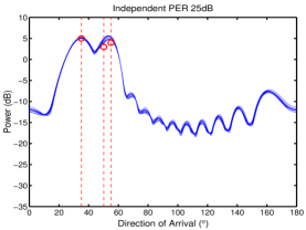
(a)	(b)
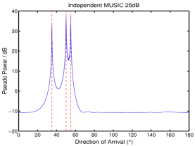
(c)	(d)

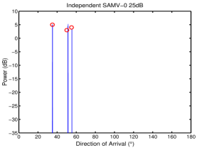
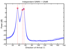
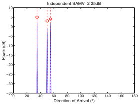
(e)	(f)	(g)
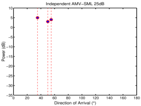
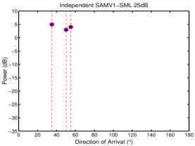
(h)	(i)	(j)

Figure 1: Source localization with a ULA of $M=12$ sensors and $N=120$ snapshots, SNR = $25$ dB: Three uncorrelated sources at $35.11^{\circ}$, $50.15^{\circ}$ and $55.05^{\circ}$, respectively, as represented by the red circles and vertical dashed lines in each plot. $10$ Monte Carlo trials are shown in each plot. Spatial estimates are shown with (a) Periodogram (PER), (b) IAA, (c) SPICE+, (d) MUSIC, (e) SAMV-0, (f) SAMV-1, (g) SAMV-2, (h) AMV-SML, (i) SAMV1-SML and (j) SAMV2-SML.

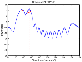
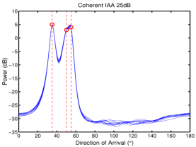
(a)	(b)
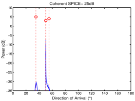
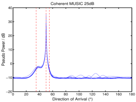
(c)	(d)

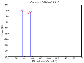
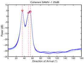
(e)	(f)	(g)
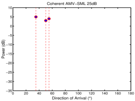
(h)	(i)	(j)

Figure 2: Source localization with a ULA of $M=12$ sensors and $N=120$ snapshots, SNR = $25$ dB: Three sources at $35.11^{\circ}$, $50.15^{\circ}$ and $55.05^{\circ}$, respectively. The first and the last source are coherent. These sources are represented by the red circles and vertical dashed lines in each plot. $10$ Monte Carlo trials are shown in each plot. Spatial estimates are shown with (a) Periodogram (PER), (b) IAA, (c) SPICE+, (d) MUSIC, (e) SAMV-0, (f) SAMV-1, (g) SAMV-2, (h) AMV-SML, (i) SAMV1-SML and (j) SAMV2-SML.

Due to the strong smearing effects and limited resolution, the PER approach fails to correctly separate the close sources at $\theta_{2}$ and $\theta_{3}$ (Figure 1(a) and Figure 2(a)). The IAA algorithm has reduced the smearing effects significantly, resulting lower sidelobe levels in Figure 1(b) and Figure 2(b). However, the resolution provided by IAA is still not high enough to separate the two close sources at $\theta_{2}$ and $\theta_{3}$.

In the scenario with independent sources, the eigen-analysis based MUSIC algorithm and existing sparse methods such as the SPICE+ algorithm, are capable of resolving all three sources in Figure 1(c)–(d), thanks to their superior resolution. However, the source coherence degrades their performances dramatically in Figure 2(c)–(d). On contrary, the proposed SAMV algorithms depicted in Figure 2(e)–(g), are much more robust against signal coherence. We observe in Figure 1–2 that the SAMV-1 approach generally provides identical spatial estimates to its IAA counterpart and this phenomenon is again revealed in Figure 3–4, which verifies the comments in Section VI. In Figure 1–2, the SAMV-0 and SAMV-2 algorithm generate high resolution sparse spatial estimates for both the independent and coherent sources. However, we notice in our simulations that the sparsest SAMV-0 algorithm requires a high SNR to work properly. Therefore, SAMV-0 is not included when comparing angle estimation mean-square-error over a wide range of SNR in Figure 3–4. From Figure 1–2, we comment that the SAMV-SML algorithms (AMV-SML, SAMV1-SML and SAMV2-SML) provide the most accurate estimates of the source locations and powers simultaneously.

Next, Figures 3–4 compare the total angle mean-square-error (MSE) of each algorithm with respect to varying SNR values for both independent and coherent sources. These DOA localization results are obtained using a $12$ element ULA and $N=16\textrm{ or }120$ snapshots. Two sources with $5$ dB and $3$ dB power at location $\theta_{1}=35.11^{\circ}$ and $\theta_{2}=50.15^{\circ}$ are present.

While calculating the MSEs for the power-based grid-dependent algorithms, only the highest two peaks in $\{\hat{p}_{k}\}_{k=1}^{K}$ are selected as the estimates of the source locations. The grid-independent SAMV-SML algorithms (AMV-SML, SAMV1-SML and SAMV2-SML) are all initialized by the SAMV-2 algorithm. Each point in Figure 3–4 is the average of $1000$ Monte Carlo trials.

Due to the severe smearing effects (already shown in Figure 1–2), the PER approach gives high total angle MSEs in Figure 3–4. Figure 3(b) shows that the SPICE+ algorithm has favorable angle estimation variance characteristics for independent sources, especially with sufficient snapshots. However, the source coherence degrades the SPICE+ performance dramatically in Figure 4. On contrary, the SAMV-2 approach offers lower total angle estimation MSE, especially for the coherent sources case, and this is also the main reason why we initialize the SAMV-SML approaches with the SAMV-2 result. Note that in Figure 3, the IAA, SAMV-1 and SAMV-2 provide similar MSEs at very low SNR, which has already been investigated in Section VI. The zero-order low SNR approximation shows that the SAMV-1 and SAMV-2 estimates are equivalent to the PER result or a scaled version of it.

We also observe that there exist the plateau effects for the power-based grid-dependent algorithms (IAA, SAMV-1, SAMV-2, SPICE+) in Figure 3–4 when the SNR are sufficiently high. These phenomena reflect the resolution limitation imposed by the direction grid detailed in Section V. Since the power-based grid-dependent algorithms estimate each source location $\theta_{\textrm{source}}$ by selecting one element from a fixed set of discrete values (i.e., the direction grid values, $\{\theta_{k}\}_{k=1}^{K}$), there always exists an estimation bias provided that the sources are not located precisely on the direction grid. Theoretically, this bias can be reduced if the adjacent distance between the grid is reduced. However, a uniformly fine direction grid with large $K$ values incurs prohibitive computational costs and is not applicable for practical applications. In lieu of increasing the value of $K$, some adaptive grid refinement postprocessing techniques have been developed (e.g., [15]) by refining this grid locally. To combat the resolution limitation without relying on additional grid refinement postprocessing, the SAMV-SML approaches employ a grid-independent one-dimensional minimization scheme, and the resulted angle estimation MSEs are significantly reduced at high SNR compared to the SAMV approaches in Figure 3–4. We also note that the MSE performances of the SAMV1-SML and SAMV2-SML approaches are identical to their AMV-SML counterpart, which verifies that the SAMV signal powers and noise variance updating formulas (Eq. 14–16) are good approximations to the ML estimates (Eq. 4–5). In the independent sources scenario in Figure 3, the MSE curves of the SAMV-SML approaches agree well with the stochastic Cramér-Rao lower bound (CRB, see, e.g., [26]) over most of the indicated range of SNR. Even with coherent sources, these SAMV-SML approaches are still asymptotically efficient and they provide lower angle estimation MSEs than competing algorithms over a wide range of SNR.

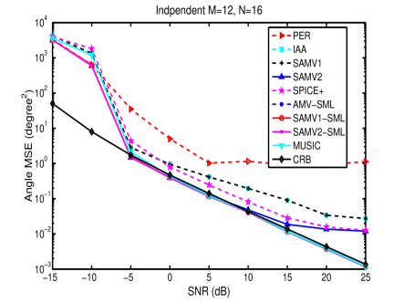
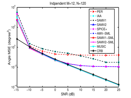
(a)	(b)

Figure 3: Source localization: Two uncorrelated sources at $35.11^{\circ}$ and $50.15^{\circ}$ with a ULA of $M=12$ sensors. (a) Total angle estimation MSE with $N=16$ snapshots and (b) total angle estimation MSE with $N=120$ snapshots.

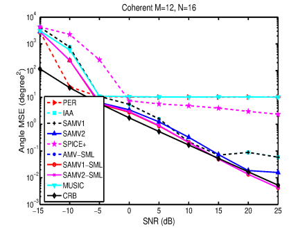
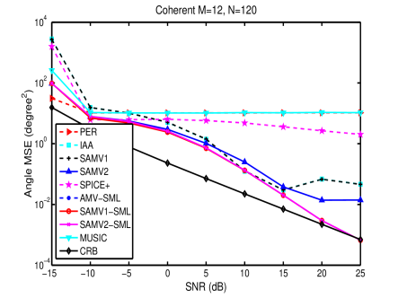
(a)	(b)

Figure 4: Source localization: Two coherent sources at $35.11^{\circ}$ and $50.15^{\circ}$ with a ULA of $M=12$ sensors. (a) Total angle estimation MSE with $N=16$ snapshots and (b) total angle estimation MSE with $N=120$ snapshots.

VII-B Active Sensing: Range-Doppler Imaging Examples

This subsection focuses on numerical examples for the SISO radar/sonar Range-Doppler imaging problem. Since this imaging problem is essentially a single-snapshot application, only algorithms that work with single snapshot are included in this comparison, namely, Matched Filter (MF, another alias of the periodogram approach), IAA, SAMV-0, SAMV-1 and SAMV-2. First, we follow the same simulation conditions as in [16]. A $30$-element P3 code is employed as the transmitted pulse, and a total of nine moving targets are simulated. Of all the moving targets, three are of $5$ dB power and the rest six are of $25$ dB power, as depicted in Figure 5(a). The received signals are assumed to be contaminated with uniform white Gaussian noise of $0$ dB power. Figure 5 shows the comparison of the imaging results produced by the aforementioned algorithms.

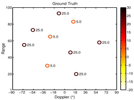
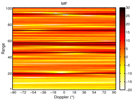
(a)	(b)
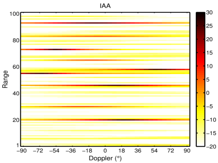
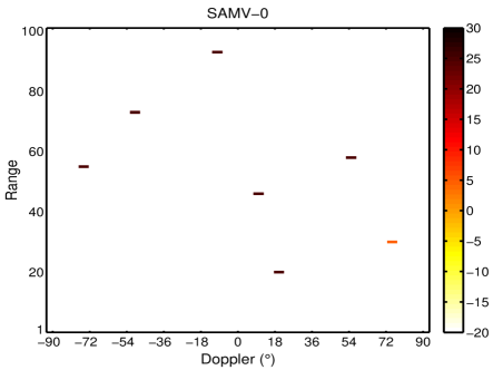
(c)	(d)
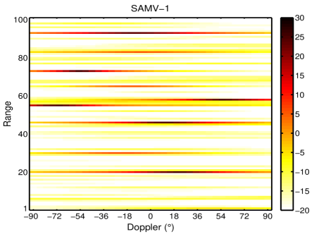
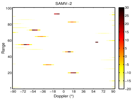
(e)	(f)

Figure 5: SISO range-Doppler imaging with three $5$ dB and six $25$ dB targets. (a) Ground Truth with power levels, (b) Matched Filter (MF), (c) IAA, (d) SAMV-0, (e) SAMV-1 and (f) SAMV-2. Power levels are all in dB.

The Matched Filter (MF) result in Figure 5(b) suffers from severe smearing and leakage effects both in the Doppler and range domain, hence it is impossible to distinguish the $5$ dB targets. On contrary, the IAA algorithm in Figure 5(c) and SAMV-1 in Figure 5(e) offer similar and greatly enhanced imaging results with observable target range estimates and Doppler frequencie. The SAMV-0 approach provides highly sparse result and eliminates the smearing effects completely, but it misses the weak $5$ dB targets in Figure 5(d), which agree well with our previous comment on its sensitivity to SNR. In Figure 5(f), the smearing effects (especially in the Doppler domain) are further attenuated by SAMV-2, compared with the IAA/SAMV-1 results. We comment that among all the competing algorithms, the SAMV-2 approach provides the best balanced result, providing sufficiently sparse images without missing weak targets.

In Figure 5(d), the three $5$ dB sources are not resolved by the SAMV-0 approach due to the excessive low SNR. After increasing the power levels of these sources to $15$ dB (the rest conditions are kept the same as in Figure 5), all the sources can be accurately resolved by the SAMV-0 approach in Figure 6(d). We comment that the SAMV-0 approach provides the most accurate imaging result provided that all sources have adequately high SNR.

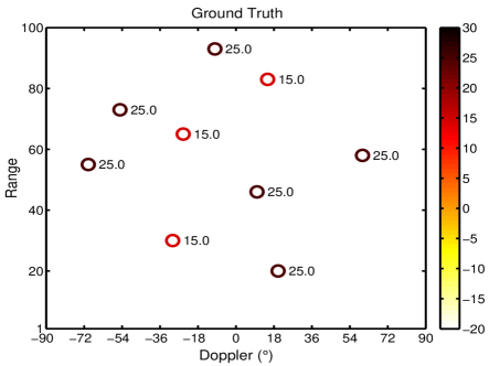
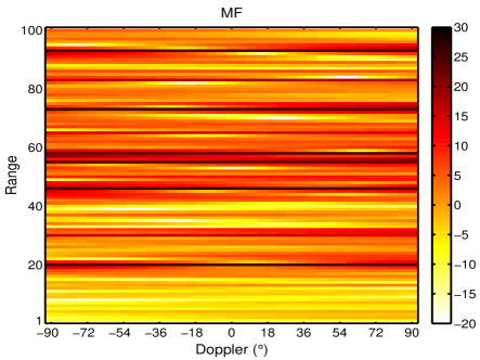
(a)	(b)
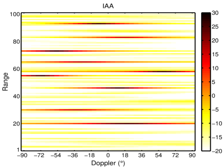
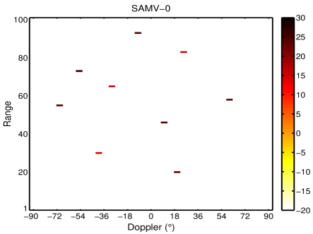
(c)	(d)
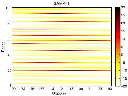
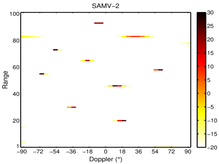
(e)	(f)

Figure 6: SISO range-Doppler imaging with three $15$ dB and six $25$ dB targets. (a) Ground Truth with power levels, (b) Matched Filter (MF), (c) IAA, (d) SAMV-0, (e) SAMV-1 and (f) SAMV-2. Power levels are all in dB.

VIII Conclusions

We have presented a series of user parameter-free array processing algorithms, the iterative SAMV algorithms, based on the AMV criterion. It has been shown that these algorithms have superior resolution and sidelobe suppression ability and are robust to practical difficulties such as insufficient snapshots, coherent source signals, without the need of any decorrelation preprocessing. Moreover, a series of grid-independent SAMV-SML approaches are proposed to combat the limitation of the direction grid. It is shown that these approaches provide grid-independent asymptotically efficient estimates without any additional grid refinement postprocessing.

Appendix A Proof of Result 1

Given $\{{\hat{p}_{k}}^{(i)}\}_{k=1}^{K}$ and $\hat{\sigma}^{(i)}$, which are the estimates of the first $K$ components and the last element of ${\bf p}$ at $i$th iteration, the matrix ${\bf R}^{(i)}={\bf A}{\bf P}^{(i)}{\bf A}^{H}+\sigma^{(i)}{\bf I}$ is known, thus the matrix ${\bf C}^{(i)}_{r}={\bf R}^{*(i)}\otimes{\bf R}^{(i)}$ is also known. For the notational simplicity, we omit the iteration index and use ${\bf C}_{r}$ instead in this section.

Define the vectorized covariance matrix of the interference and noise as

$${\bf r}^{\prime}_{k}\stackrel{{\scriptstyle{\rm def}}}{{=}}{\bf r}-p_{k}\bar{\bf a}_{k},\;k=1,\ldots,K.$$

Assume that ${\bf r}^{\prime}_{k}$ is known and substitute ${\bf r}^{\prime}_{k}+p_{k}\bar{\bf a}_{k}$ for ${\bf r}$ in (3), minimizing (3) is equivalent to minimizing the following cost function

$$f(p_{k})=[{\bf r}_{N}-p_{k}\bar{\bf a}_{k}]^{H}{\bf C}_{r}^{-1}[{\bf r}_{N}-p_{k}\bar{\bf a}_{k}]-[{\bf r}_{N}-p_{k}\bar{\bf a}_{k}]^{H}{\bf C}_{r}^{-1}{\bf r}^{\prime}_{k}-{\bf r}^{{}^{\prime}H}_{k}{\bf C}_{r}^{-1}[{\bf r}_{N}-p_{k}\bar{\bf a}_{k}]+{\bf r}^{{}^{\prime}H}_{k}{\bf C}_{r}^{-1}{\bf r}^{{}^{\prime}}_{k}$$ (36)

Note that ${\bf r}^{{}^{\prime}}_{k}$ does not depend on $p_{k}$. Differentiating (3) with respect to ${p}_{k}$ and setting the results to zero, we get

$$\hat{p}_{k}=\frac{1}{\bar{\bf a}^{H}_{k}{\bf C}_{r}^{-1}\bar{\bf a}_{k}}\left(\bar{\bf a}^{H}_{k}{\bf C}_{r}^{-1}{\bf r}_{N}-\bar{\bf a}^{H}_{k}{\bf C}_{r}^{-1}{\bf r}^{\prime}_{k}\right),\;k=1,\ldots,K+1.$$ (37)

Replacing ${\bf r}^{\prime}_{k}$ with its definition in (37) yields

$$\hat{p}_{k}=\frac{1}{\bar{\bf a}^{H}_{k}{\bf C}_{r}^{-1}\bar{\bf a}_{k}}\left(\bar{\bf a}^{H}_{k}{\bf C}_{r}^{-1}{\bf r}_{N}+p_{k}\bar{\bf a}^{H}_{k}{\bf C}_{r}^{-1}\bar{\bf a}_{k}-\bar{\bf a}^{H}_{k}{\bf C}_{r}^{-1}{\bf r}\right).$$ (38)

Using the following identities (see, e.g., [32, Th. 7.7, 7.16]),

$${\rm vec}({\bf A}{\bf B}{\bf C}) = ({\bf C}^{T}\otimes{\bf A}){\rm vec}({\bf B}),$$ (39)

$$({\bf A}\otimes{\bf B})\otimes({\bf C}\otimes{\bf D}) = {\bf A}{\bf C}\otimes{\bf B}{\bf D},$$ (40)

Eq. (38) can be simplified as

$$\hat{p}_{k} = \frac{{\bf a}^{H}_{k}{\bf R}^{-1{}}{\bf R}_{N}{\bf R}^{-1{}}{\bf a}_{k}}{({\bf a}^{H}_{k}{\bf R}^{-1{}}{\bf a}_{k})^{2}}+{p}_{k}-\frac{1}{{\bf a}^{H}_{k}{\bf R}^{-1{}}{\bf a}_{k}},\;k=1,\ldots,K,$$ (41)

$$\hat{\sigma}=\hat{p}_{K+1} = \frac{1}{{\rm Tr}({\bf R}^{-2})}\left({\rm Tr}({\bf R}^{-2}{\bf R}_{N})+\sigma{\rm Tr}({\bf R}^{-2})-{\rm Tr}({\bf R}^{-1})\right).$$ (42)

Computing $\hat{p}_{k}$ and $\hat{\sigma}$ requires the knowledge of $p_{k}$, $\sigma$, and ${\bf R}$. Therefore, this algorithm must be implemented iteratively as is detailed in Table 1.

Appendix B Proof of Result 2

Define the covariance matrix of the interference and noise as

$${\bf Q}_{k}\stackrel{{\scriptstyle{\rm def}}}{{=}}{\bf R}-p_{k}{\bf a}_{k}{\bf a}^{H}_{k},\;k=1,\ldots,K.$$ (43)

Applying the matrix inversion lemma to (43) yields

$${\bf R}^{-1}={\bf Q}^{-1}_{k}-p_{k}\beta_{k}{\bf b}_{k}{\bf b}^{H}_{k},\;k=1,\ldots,K,$$ (44)

where ${\bf b}_{k}\stackrel{{\scriptstyle{\rm def}}}{{=}}{\bf Q}^{-1}_{k}{\bf a}_{k}$ and $\beta_{k}\stackrel{{\scriptstyle{\rm def}}}{{=}}(1+p_{k}{\bf a}^{H}_{k}{\bf Q}^{-1}_{k}{\bf a}_{k})^{-1}$. Since

$${\rm Tr}({\bf R}^{-1}{\bf R}_{N}) = {\rm Tr}({\bf Q}^{-1}_{k}{\bf R}_{N})-p_{k}\beta_{k}{\bf b}^{H}_{k}{\bf R}_{N}{\bf b}_{k},$$ (45)

and using the algebraic identity $\det({\bf I}+{\bf A}{\bf B})=\det({\bf I}+{\bf B}{\bf A})$, we obtain

$$\ln(\det({\bf R})) = \ln(\det({\bf Q}_{k}+p_{k}{\bf a}_{k}{\bf a}^{H}_{k}))=\ln\left[(1+p_{k}{\bf a}^{H}_{k}{\bf Q}^{-1}_{k}{\bf a}_{k})\det({\bf Q}_{k})\right]$$

$$= \ln(\det({\bf Q}_{k}))-\ln(\beta_{k}).$$

Substituting (45) and (B) into the ML function (6) yields

$$\mathcal{L}({\bf p}) = \ln(\det({\bf Q}_{k}))+{\rm Tr}({\bf Q}^{-1}_{k}{\bf R}_{N})-\left(\ln(\beta_{k})+p_{k}\beta_{k}({\bf b}^{H}_{k}{\bf R}_{N}{\bf b}_{k})\right)$$ (47)

$$= \mathcal{L}({\bf p}_{-k})-l(p_{k}),$$

with

$$l(p_{k})\stackrel{{\scriptstyle{\rm def}}}{{=}}\ln\left(\frac{1}{1+p_{k}\alpha_{1,k}}\right)+p_{k}\frac{\alpha^{N}_{2,k}}{1+p_{k}\alpha_{1,k}},$$ (48)

where $\alpha_{1,k}\stackrel{{\scriptstyle{\rm def}}}{{=}}({\bf a}^{H}_{k}{\bf Q}^{-1}_{k}{\bf a}_{k})^{-1}$ and $\alpha^{N}_{2,k}\stackrel{{\scriptstyle{\rm def}}}{{=}}({\bf a}^{H}_{k}{\bf Q}^{-1}_{k}{\bf R}_{N}{\bf Q}^{-1}_{k}{\bf a}_{k})^{-1}$. The objective function has now been decomposed into $\mathcal{L}({\bf p}_{-k})$, the marginal likelihood with $p_{k}$ excluded, and $l(p_{k})$, where terms concerning $p_{k}$ are conveniently isolated. Consequently, minimizing (6) with respect to $p_{k}$ is equivalent to minimizing the function (48) with respect to the parameter $p_{k}$.

It has been proved in [16, Appendix, Eqs. (27) and (28)] that the unique minimizer of the cost function (48) is

$$\hat{p}_{k}=\frac{{\bf a}^{H}_{k}{\bf Q}^{-1}_{k}({\bf R}_{N}-{\bf Q}_{k}){\bf Q}^{-1}_{k}{\bf a}_{k}}{({\bf a}^{H}_{k}{\bf Q}^{-1}_{k}{\bf a}_{k})^{2}},\;k=1,\ldots,K.$$ (49)

We note that $\hat{\bf p}$ is strictly positive if ${\bf a}^{H}_{k}{\bf Q}^{-1}_{k}{\bf R}_{N}{\bf Q}^{-1}_{k}{\bf a}_{k}>{\bf a}^{H}_{k}{\bf Q}^{-1}_{k}{\bf a}_{k}$. Using (44), we have

$${\bf a}^{H}_{k}{\bf Q}^{-1}_{k}{\bf a}_{k} = \gamma_{k}({\bf a}^{H}_{k}{\bf R}^{-1}{\bf a}_{k}),$$ (50)

$${\bf a}^{H}_{k}{\bf Q}^{-1}_{k}{\bf R}_{N}{\bf Q}^{-1}_{k}{\bf a}_{k} = \gamma^{2}_{k}({\bf a}^{H}_{k}{\bf R}^{-1}{\bf R}_{N}{\bf R}^{-1}{\bf a}_{k}),$$ (51)

where $\gamma_{k}\stackrel{{\scriptstyle{\rm def}}}{{=}}1+p_{k}{\bf a}^{H}_{k}{\bf Q}^{-1}_{k}{\bf a}_{k}$. Substituting (50) and (51) into (49), we obtain the desired expression

$$\hat{p}_{k}=\frac{{\bf a}^{H}_{k}{\bf R}^{-1}({\bf R}_{N}-{\bf R}){\bf R}^{-1}{\bf a}_{k}}{({\bf a}^{H}_{k}{\bf R}^{-1}{\bf a}_{k})^{2}}+p_{k}=\frac{{\bf a}^{H}_{k}{\bf R}^{-1}{\bf R}_{N}{\bf R}^{-1}{\bf a}_{k}}{({\bf a}^{H}_{k}{\bf R}^{-1}{\bf a}_{k})^{2}}+p_{k}-\frac{1}{{\bf a}^{H}_{k}{\bf R}^{-1}{\bf a}_{k}}.$$ (52)

Differentiating (6) with respect to $\sigma$ and setting the result to zero, we obtain

$$\hat{\sigma}=\frac{{\rm Tr}{({\bf R}^{-1}({\bf R}_{N}-\bar{\bf R}){\bf R}^{-1}})}{{\rm Tr}{({\bf R}^{-2})}},$$ (53)

and after substituting ${\bf R}-\sigma{\bf I}$ for $\bar{\bf R}$ in the above equation,

$$\hat{\sigma}=\frac{{\rm Tr}({\bf R}^{-1}({\bf R}_{N}-{\bf R}){\bf R}^{-1})}{{\rm Tr}({\bf R}^{-2})}+\sigma={\rm Tr}({\bf R}^{-2}{\bf R}_{N})/{{\rm Tr}{({\bf R}^{-2})}}+{\sigma}-{\rm Tr}({\bf R}^{-1})/{{\rm Tr}{({\bf R}^{-2})}}.$$ (54)

Computing $\hat{p}_{k}$ and $\hat{\sigma}$ requires the knowledge of $p_{k}$, $\sigma$, and ${\bf R}$. Therefore, the algorithm must be implemented iteratively as is detailed in Result 1.

Appendix C Proof of Result 3

Differentiating (18) with respect to ${p}_{k}$ and setting the result to zero, we get

$${p}^{(i+1)}_{k}=\frac{\bar{\bf a}^{H}_{k}{\bf C^{\prime}}^{-1}_{k}{\bf r}_{N}}{\bar{\bf a}^{H}_{k}{\bf C^{\prime}}^{-1}_{k}\bar{\bf a}_{k}}.$$ (55)

Applying the matrix inversion lemma to ${\bf C^{\prime}}_{k}$, the numerator and denominator of Eq. (55) can be expressed respectively, as

$$\bar{\bf a}^{H}_{k}{\bf C^{\prime}}^{-1}_{k}{\bf r}_{N} = w_{k}(\bar{\bf a}^{H}_{k}{\bf C}^{-1}_{r}{\bf r}_{N}),$$

$$\bar{\bf a}^{H}_{k}{\bf C^{\prime}}^{-1}_{k}\bar{\bf a}_{k} = w_{k}(\bar{\bf a}^{H}_{k}{\bf C}^{-1}_{r}\bar{\bf a}_{k}),$$

where $w_{k}\stackrel{{\scriptstyle{\rm def}}}{{=}}1+\frac{\bar{\bf a}^{H}_{k}{\bf C}^{-1}_{r}\bar{\bf a}_{k}}{1/p^{2}_{k}+\bar{\bf a}^{H}_{k}{\bf C}^{-1}_{r}\bar{\bf a}_{k}}$.

Thus,

$${p}^{(i+1)}_{k} = \frac{\bar{\bf a}^{H}_{k}{\bf C^{\prime}}^{-1}_{k}{\bf r}_{N}}{\bar{\bf a}^{H}_{k}{\bf C^{\prime}}^{-1}_{k}\bar{\bf a}_{k}}=\frac{\bar{\bf a}^{H}_{k}{\bf C}^{-1}_{r}{\bf r}_{N}}{\bar{\bf a}^{H}_{k}{\bf C}^{-1}_{r}\bar{\bf a}_{k}},\;k=1,\ldots,K+1.$$ (56)

Using the Kronecker product properties and the identities (39) and (40), with ${\bf A}={\bf B}={\bf R}$ and ${\bf C}={\bf R}_{N}$, the numerator and denominator of Eq. (56) can be expressed respectively, as

$$\bar{\bf a}^{H}_{k}{\bf C}^{-1}_{r}{\bf r}_{N} = {\bf a}^{H}_{k}{\bf R}^{-1}{\bf R}_{N}{\bf R}^{-1}{\bf a}_{k},\;k=1,\ldots,K,$$ (57)

$$\bar{\bf a}^{H}_{k}{\bf C}^{-1}_{r}\bar{\bf a}_{k} = ({\bf a}^{H}_{k}{\bf R}^{-1}{\bf a}_{k})^{2},\;k=1,\ldots,K,$$ (58)

and

$$\bar{\bf a}^{H}_{K+1}{\bf C}^{-1}_{r}{\bf r}_{N} = {\rm Tr}({\bf R}^{-2}{\bf R}_{N}),$$ (59)

$$\bar{\bf a}^{H}_{K+1}{\bf C}^{-1}_{r}\bar{\bf a}_{K+1} = {\rm Tr}({\bf R}^{-2}).$$ (60)

Therefore, dividing (57) by (58) gives (14), and dividing (59) by (60) yields (15).

References

- [1] D. L. Donoho, M. Elad, and V. N. Temlyakov, “Stable recovery of sparse overcomplete representations in the presence of noise,” IEEE Trans. on Infor.Theory, vol. 52, no. 1, pp. 6–18, Jan. 2006.
- [2] E. Candes, J. Romberg, T. Tao, “Stable signal recovery from incomplete and inaccurate measurements,” Communications on Pure and Applied Mathematics, vol. 59, pp. 1207–1223, 2006.
- [3] J. A. Tropp, “Just relax: convex programming methods for identifying sparse signals in noise,” IEEE Trans. Infor. Theory, vol. 52, no. 3, pp. 1030–1051, Mar. 2006.
- [4] D. L. Donoho and M. Elad, “Optimally sparse representation in general (nonorthogonal) dictionaries via minimization,” Proc. Nat. Acad. Sci., vol. 100, pp. 2197–2202, 2003.
- [5] I. F. Gorodnitsky and B. D. Rao, “Sparse signal reconstruction from limited data using FOCUSS: A re-weighted minimum norm algorithm,” IEEE Trans. Signal Process., vol. 45, no. 3, pp. 600–616, Mar. 1997.
- [6] B. D. Rao, K. Engan, S. F. Cotter, J. Palmer, K. Kreutz-Delgado, “Subset selection in noise based on diversity measure minimization,” IEEE Trans. on Signal. Process., vol. 51, no. 3, pp. 760–770, 2003.
- [7] I. J. Fevrier, S. B. Gelfand, and M. P. Fitz, “Reduced complexity decision feedback equalization for multipath channels with large delay spreads,” IEEE Trans. Commun., vol. 47, pp. 927–937, June 1999.
- [8] S. F. Cotter and B. D. Rao, “Sparse channel estimation via Matching Pursuit with application to equalization,” IEEE Trans. Commun., vol. 50, pp. 374–377, Mar. 2002.
- [9] J. Ling, T. Yardibi, X. Su, H. He, and J. Li, “Enhanced channel estimation and symbol detection for high speed Multi-Input Multi-Output underwater acoustic communications,” Journal of the Acoustical Society of America, vol. 125, pp. 3067–3078, May 2009.
- [10] C. R. Berger, S. Zhou, J. Preisig, and P. Willett, “Sparse channel estimation for multicarrier underwater acoustic communication: From subspace methods to compressed sensing,” IEEE Trans. on Signal. Process., vol. 58, no. 3, pp. 1708–1721, March 2010.
- [11] M. Cetin and W. C. Karl, “Feature-enhanced synthetic aperture radar image formation based on nonquadratic regularization,” IEEE Trans. Image Process., vol. 10, no. 4, pp. 623–631, April 2001.
- [12] Z. Chen, X. Tan, M. Xue, and J. Li, “Bayesian SAR imaging,” In Proc. of SPIE on Technologies and Systems for Defense and Security, Orlando, FL, April 2010.
- [13] W. Roberts, P. Stoica, J. Li, T. Yardibi, and F. A. Sadjadi, “Iterative adaptive approaches to MIMO radar imaging,” IEEE Journal on Selected Topics in Signal Proc., vol. 4, no. 1, pp. 5–20, 2010.
- [14] C. D. Austin, E. Ertin, and R. L. Moses, “Sparse signal methods for 3-D radar imaging,” IEEE Trans. Signal Process. vol. 5, no. 3, pp. 408–423, June 2011.
- [15] D. M. Malioutov, M. Cetin, and A. S. Willsky, “A sparse signal reconstruction perspective for source localization with sensor arrays,” IEEE Trans. Signal Processing, vol. 53, no. 8, pp. 3010–3022, August 2005.
- [16] T. Yardibi, J. Li, P. Stoica, M. Xue, and A. B. Baggeroer, “Source localization and sensing: A nonparametric iterative adaptive approach based on weighted least squares,” IEEE Trans. Aerosp. Electron. Syst., vol. 46, pp. 425–443, 2010.
- [17] R. O. Schmidt, “Multiple emitter location and signal parameter estimation,” IEEE Trans. on Antennas and Prop., vol. 34, no. 3, pp. 276–280, 1986.
- [18] R. Roy, A. Paulraj, and T. Kailath, “ESPRIT–A subspace rotation approach to estimation of parameters of cisoids in noise,” IEEE Transactions on Acoustics, Speech and Signal Processing, vol. 34, no. 5, pp. 1340–1342, 1986.
- [19] S. U. Pillai and B. H. Kwon, “Forward/backward spatial smoothing techniques for coherent signal identification,” IEEE Trans. Acoustic, Speech, Signal Processing, vol. 37, pp. 8–15, 1989.
- [20] P. Stoica, P. Babu, and J. Li, “SPICE: A sparse covariance-based estimation method for array processing,” IEEE Trans. Signal Processing, vol. 59, no. 2, pp. 629–638, Feb. 2011.
- [21] P. Stoica, P. Babu, and J. Li, “New method of sparse parameter estimation in separable models and its use for spectral analysis of irregularly sampled data,” IEEE Transactions on Signal Processing, vol. 59, no. 1, pp. 35–47, 2011.
- [22] B. Porat and B. Friedlander, “Asymptotic accuracy of ARMA parameter estimation methods based on sample covariances,” Proc.7th IFAC/IFORS Symposium on Identification and System Parameter Estimation, York, 1985.
- [23] P. Stoica, B. Friedlander and T. Söderström, “An approximate maximum approach to ARMA spectral estimation,” in Proc. Decision and control, Fort Lauderdale, 1985.
- [24] A. B. Gershman, A. L. Matveyev, and J. F. Bohme, “ML estimation of signal power in the presence of unknown noise field–simple approximate estimator and explicit Cramer-Rao bound,” Proc. IEEE Int. Conf. on Acoust., Speech, and Signal Processing (ICASSP’95), pp. 1824–1827, Detroit, Apr. 1995.
- [25] A. B. Gershman, V. I. Turchin, and R. A. Ugrinovsky, “Simple maximum likelihood estimator for structured covariance parameters,” Electron. Lett., vol. 28, no. 18, pp. 1677–1678, Aug. 1992.
- [26] P. Stoica and A. Nehorai, “Performance study of conditional and unconditional direction of arrival estimation,” IEEE Trans. Acoust., Speech, Signal Processing, vol. 38, pp. 1783–1795, Oct. 1990.
- [27] H. Abeida and J. P. Delmas, “Efficiency of subspace-based DOA estimators,” Signal Process., vol. 87, pp. 2075–2084, 2007.
- [28] J. P. Delmas, “Asymptotically minimum variance second-order estimation for non-circular signals with application to DOA estimation,” IEEE Trans. Signal Processing, vol. 52, no. 5, pp. 1235–1241, May 2004.
- [29] H. Abeida and J. P. Delmas, “MUSIC-like estimation of direction of arrival for non-circular sources,” IEEE Trans. Signal Processing, vol. 54, no. 7, pp. 2678–2690, Jul. 2006.
- [30] P. Stoica and R. Moses, Spectral Analysis of Signals, Upper Saddle River, NJ: Prentice-Hall, 2005.
- [31] T. W. Anderson, An Introduction to Multivariate Statistical Analysis, John Wiley & Sons, Inc., 1958.
- [32] J. R. Schott, Matrix Analysis for Statistics, New York: Wiley, 1980.
- [33] J. A. Nelder and R. Mead, “A simplex method for function minimization,” Computer Journal, vol. 7, pp. 308–313, 1965.
- [34] Q. Zhang, H. Abeida, M. Xue, W. Rowe, and J. Li, “Fast implementation of sparse iterative covariance-based estimation for array processing,” in Signals, Systems and Computers (ASILOMAR), 2011 Conference Record of the Forty Fifth Asilomar Conference on. IEEE, 2011, pp. 2031–2035.
- [35] Q. Zhang, H. Abeida, M. Xue, W. Rowe, and J. Li, “Fast implementation of sparse iterative covariance-based estimation for source localization,” The Journal of the Acoustical Society of America, vol. 131, no. 2, pp. 1249–1259, 2012.