Generating Realistic Geology Conditioned on Physical Measurements
with Generative Adversarial Networks
Abstract
An important problem in geostatistics is to build models of the subsurface of the Earth given physical measurements at sparse spatial locations. Typically, this is done using spatial interpolation methods or by reproducing patterns from a reference image. However, these algorithms fail to produce realistic patterns and do not exhibit the wide range of uncertainty inherent in the prediction of geology. In this paper, we show how semantic inpainting with Generative Adversarial Networks can be used to generate varied realizations of geology which honor physical measurements while matching the expected geological patterns. In contrast to other algorithms, our method scales well with the number of data points and mimics a distribution of patterns as opposed to a single pattern or image. The generated conditional samples are state of the art.
1 Introduction
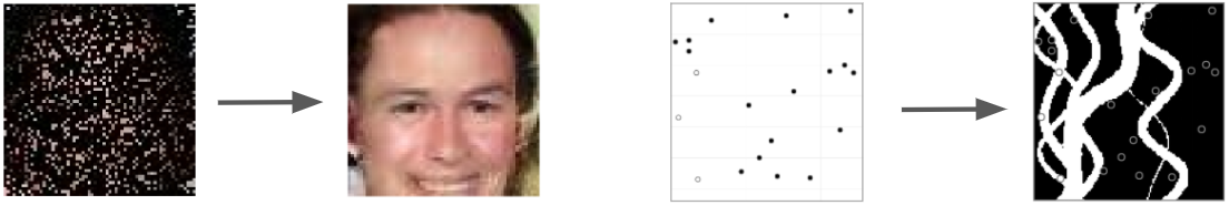
Modeling geology based on sparse physical measurements is key for several use cases including natural resource management, natural hazard identification and geological process quantification. The modeling process involves inferring geological properties, such as rock type, over a wide area given measurements at only a small number of locations. Several tools exist for creating geological models, one of the most important being geostatistics (Deutsch et al. (1992)). Early geostatistics algorithms mainly used spatial linear interpolation or performed simulation of geological attributes by assuming these attributes follow Gaussian distributions (Cressie (1990)). Most geological patterns, however, are non Gaussian and highly non linear (Fig. 1). To overcome these limitations, geostatistical approaches have been developed to simulate complex geological patterns based on a training image (Strebelle (2002); Zhang et al. (2006)). These methods aim to generate geological models by extracting patterns from the training image and anchoring them to physical measurements at known locations. However, these algorithms fail to produce realistic non linear patterns and do not exhibit the variability and uncertainty of geological inference.

In this paper, we propose a novel approach, based on deep generative models, for generating realistic geological models that can model a distribution of images and reproduce geological patterns while having the flexibility to honor physical measurements. Despite the recent progress in generative modeling, there have only been few examples of geological applications, all of which aim to generate data in an unconstrained fashion (Mosser et al. (2017a, b); Chan and Elsheikh (2017)). By establishing a connection between semantic inpainting and modeling geology, we show how we can generate realistic geological realizations constrained by physical measurements at various spatial locations. To the best of our knowledge, this is the first time the connection between semantic inpainting algorithms and geomodelling has been made. We hope this opens an avenue for generating realistic subsurface geological models constrained by a variety of physical measurements in a seamless fashion.
While the problem we study is one of geology, we believe our approach is applicable to many fields. Specifically, several tasks in spatio-temporal statistics (Cressie and Wikle (2015)) could benefit from our method, with applications to energy, climate, the environment and agriculture. In general, our algorithm can be used to solve the task of inferring geospatial patterns of quantities such as temperature, pressure, humidity and porosity from sparse measurements. As an example of an alternative use case we have applied our algorithm to satellite images of river deltas.
2 Method
2.1 Problem Statement
Given a number of true physical measurements and a distribution of geological patterns (e.g. a large set of images), we would like to generate realizations of the geology which honor the physical measurements while producing realistic geological patterns. More specifically, suppose that a specific area is known to have, for example, fluvial geological patterns (see Fig. 1). Suppose also that, at various spatial locations , the type of the rock has been measured, i.e. we have set of tuples of the form . Given these measurements, we wish to infer the rock type at all locations such that:
-
1.
The resulting realizations are realistic (i.e. match the distribution of geological patterns)
-
2.
The resulting realizations honor the physical measurements
In this paper we restrict ourselves to the case of fluvial patterns with binary measurements (i.e. there are only two types of rock present), although it is easy to extend this to the general case. Specifically, we have a distribution of binary images where and a set of binary measurements where . Our goal is to generate samples such that for . This approach is illustrated in Fig. 2.

2.2 Combining Semantic Inpainting and Geology
The above problem is closely related to semantic inpainting. Semantic inpainting is the task of filling in missing regions of an image using the surrounding pixels and a prior on what the images should look like. Recent semantic inpainting algorithms have taken advantage of deep generative models to create realistic infillings of various types of images (Pathak et al. (2016); Yeh et al. (2016); Li et al. (2017)). Yeh et al. (2016) in particular propose a framework for semantic inpainting based on Generative Adversarial Networks (GAN) (Goodfellow et al. (2014)). GANs are generative models composed of a generator and discriminator each parametrized by a neural network. is trained to map a latent vector into an image , while is trained to map an image to the probability of it being real (as opposed to generated). The networks are trained adversarially by optimizing the loss
After training on data drawn from a distribution , will be able to generate samples similar to those from , by sampling and mapping . Using a trained and , we would like to generate realistic images conditioned on a set of known pixel values . This can be achieved by fixing the weights of and and optimizing to generate realistic samples based on the known pixel values. In order to generate realistic samples we would like the samples to be close to , i.e. we would like to generate samples such that the discriminator assigns high probability to . This idea is formalized through the prior loss. We would also like the samples to honor the pixel values , i.e. we want the generated to match at the known pixel locations. This is formalized through the context loss.

Prior loss: The prior loss penalizes unrealistic images. Since was trained to assign high probability to realistic samples, the prior loss is chosen as
Context loss: The context loss penalizes mismatch between generated samples and known pixels . Denoting by the masking matrix (which has value 1 at the known points and 0 otherwise), the context loss is defined by Yeh et al. (2016) as
Since the set of known pixels is very sparse, we modify the objective by expanding the mask . Specifically, for every unmasked value, i.e. for every such that , we modify the neighboring pixels within a set radius to have value
which can be thought of as changing the mask from imposing a hard constraint to a smooth constraint. We perform a corresponding expansion for the set of known pixel values (see Fig. 3). This encourages the generator to output samples which not only match the known pixels but also produce similar values around the known pixels. This modification was found to facilitate the optimization of , especially when and were very sparse. Denoting by the expanded weighted masking matrix and by the expanded pixels, the modified context loss can be written as
Total loss The total loss is defined as the weighted sum of the prior loss and context loss
| (1) |
where controls the tradeoff between generating realistic images and matching the known pixel values.
We can now establish a connection between semantic inpainting and generating realizations of geology conditioned on physical measurements. We let be the distribution of fluvial patterns and we let the set of known pixel values be the set of known physical measurements at various locations. By randomly initializing and minimizing we can then obtain various realizations of the geology that are realistic while honoring the physical measurements (the relationship between using different initializations of and generating different realizations of the geology is discussed in more detail in Section 3.2). The final algorithm for generating a realization conditioned on physical measurements can then be described as follows. Given distribution of fluvial patterns , measurements :
-
1.
Train and on
-
2.
Initialize randomly
-
3.
Compute by minimizing
-
4.
Return sample
.
2.3 Generating Data
To train and we require a large dataset of geological patterns. In order to create such a dataset we take advantage of another family of geomodelling approaches called object-based models (OBM). OBMs are capable of generating very realistic geobodies based on distributions of geometric shapes using marked point processes (Deutsch and Wang (1996)). Note that these models can also be conditioned to physical measurements using Markov Chain Monte Carlo (MCMC) algorithms (Holden et al. (1998)). Even though OBMs are good at producing realistic geobodies, conditioning on dense data locations is very difficult and extremely slow and often fails to converge in MCMC (Skorstad et al. (1999); Hauge et al. (2007)).
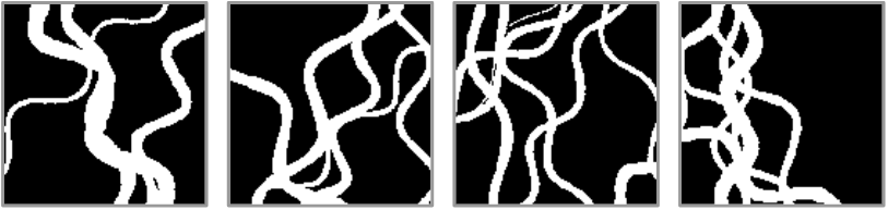
We use OBM to generate a training set of 5000 images of fluvial patterns. Each image has dimension 128 by 128 and is binary, with 1 corresponding to channels and 0 corresponding to background (i.e. two different types of rock). More details on data generation are described in the appendix. Examples of the training data are shown in Fig. 5(a).

3 Experiments
3.1 Unconditional model
We use a DC-GAN architecture (Radford et al. (2015)) for the discriminator and generator and train an unconditional model (i.e. a model that freely generates fluvial patterns without being restricted by physical measurements) on the dataset of 5000 images (see appendix for details of model architecture and training).
In order to verify that the model has learnt to generate realistic and varied samples, we perform several checks. Firstly, we visually inspect samples from the model (see Fig. 5(b)). The samples are almost indistinguishable from the true data and embody a lot of the properties of the data, e.g. the channels remain connected, the patterns are meandering and there is a large diversity suggesting the model has learnt a wide distribution of the data. Secondly, since the training images were generated by OBM, we know some of the statistics the model should satisfy (see appendix). For example, the ratio of white pixels to black pixels is a generative factor (and was chosen to be 0.25). Sampling a 1000 images from , and calculating the ratio of white to black pixels we obtain the same ratio within 1%. In addition, to ensure the channels are well distributed, we average a 1000 generated images and check that the pixel values are approximately 0.25 everywhere (see Fig. 6(a)). Finally, we can also perform traversals in latent space to ensure the model has learnt a good approximation of the data manifold. We would for example expect the changes over the latent space to be smooth and not disconnect any channels. This is shown in Fig. 6(b).


3.2 Conditional model
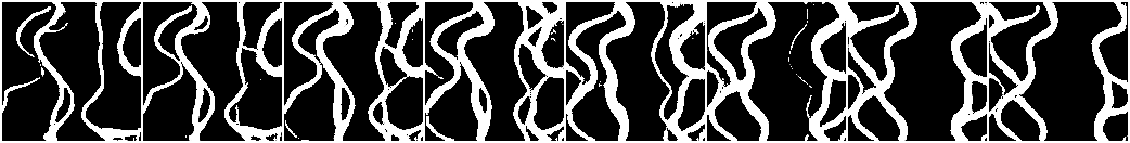
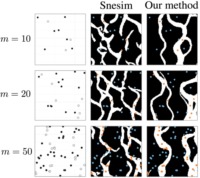
Using the unconditional GAN, we can create samples conditioned on measurements by minimizing the loss specified in equation (1). To do this, we take a fluvial image and randomly select measurement locations and mask the rest of the input. We then randomly initialize several and minimize for each of them using Adam (Kingma and Ba (2014)). This results in a set of each corresponding to a local minimum of . Each of the is mapped to a realization such that the honor the physical measurements, have realistic geological patterns and each correspond to different realizations. The idea is that different initializations will lead to different minima of and in turn a variety of samples all satisfying the constraints. Examples of this are shown in Fig. 7. As can be seen, the samples produced have high quality (the channels remain connected, the images look realistic) and satisfy the constraints while being fairly diverse. The samples produced are at least comparable to the current state of the art (see Fig. 8). Further, since the model captures patterns from a distribution of images as opposed to a single training image, the generated samples exhibit a variety of channel widths and curvatures which current algorithms cannot achieve.

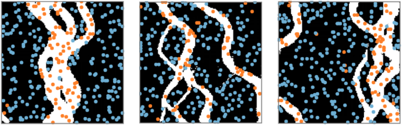
3.2.1 Large number of measurements
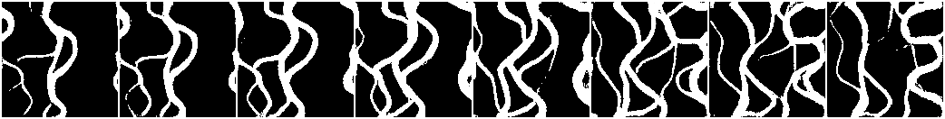
For most geostatistical modeling algorithms, increasing the number of measurements to condition on, degrades performance and increases runtime (Strebelle (2002); Zhang et al. (2006)). In particular, the generated images often become unrealistic as more data constraints are added. This is not the case for our algorithm and we are able to generate realistic patterns over a wide number of measurements from sparse to dense. Results are shown in Fig. 9(a).
3.2.2 Failure cases
Minimizing can sometimes lead to poor minima and in turn samples that are either unrealistic or do not satisfy the measurement constraints. We have included examples of this in Fig. 9(b).

3.2.3 Sample diversity
While the unconditional model exhibits large sample diversity, this is not always the case for the conditional samples. The conditional samples created are realistic and honor the physical measurements but may lack diversity. The variety of samples is based on the variety of local minima of and random initializations of may end up in the same local minimum, resulting in the same sample. It would be interesting to build semantic inpainting algorithms based on true sampling and not on solving an optimization problem. To the best of our knowledge, creating models that can simultaneously (a) generate realistic images, (b) honor constraints, (c) exhibit high sample diversity is an open problem.
3.2.4 Application to Satellite Images

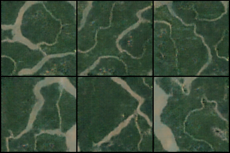

To demonstrate the wide applicability of our method we also trained a model on satellite images from the Landsat dataset (USGS (2018)). We collected 3000 satellite images from the Ganges delta in Bangladesh and India, which is a region containing a wide variety of fluvial patterns. We trained the same model that was used for the geological application on 128 by 128 versions of these satellite images. Examples of real and generated images are shown in Fig. 10(a) and 10(b).
We then randomly fixed the location of a number of known measurements. For example, a certain latitude and longitude would correspond to a point containing water and another to a point containing land. In a similar fashion to the geological application, we then minimized the loss to match the generated patterns with the known measurements. Results are shown in Fig. 11. As can be seen, the results are convincing: the generated samples look realistic while honoring the sparse measurement constraints.
While we have applied our method to generate constrained geological and satellite data, we believe the applicability of our method goes beyond this and we hope it will be used on other types of geospatial data in fields such as energy, climate, environment and agriculture.
4 Related Work
Strebelle (2002) proposed an algorithm, called snesim, based on a single training image. The algorithm works by scanning a training image and storing all the training patterns in a search tree. The simulation then proceeds by reproducing the complex patterns from the training image by inferring a local probability density function from scanning the search tree.
Zhang et al. (2006) proposed another approach based on filters. The algorithm simulates patterns from a training image by matching them with filters. A fixed set of filters is used to scan the training image, classifying training patterns by their filter scores (corresponding to convolutions of the filter with a patch of the training image). Each filter sees different aspects of the patterns in the image, e.g. an average filter for pattern location, a gradient filter for boundary detection and a curvature filter for second order changes. The simulation then proceeds in a sequential manner by visiting each pixel randomly and patching the patterns closest to the training image while honoring the previously simulated patches and measurements.
These algorithms have the flexibility of honoring measurements while reasonably capturing patterns from a training image. However, it is impractical to use these algorithms with several training images and so the simulations fail to correctly reflect the inherent uncertainty of geological predictions. Additionally, the generated samples are often not realistic, for example containing broken channels even when the training image contains only connected channels.
Chan and Elsheikh (2017) propose an approach for parameterizing a geological model using GANs. The authors use a single training image and split it into smaller patches to be used as a training set. In contrast, we use several training images with wide uncertainty and generate large coherent realizations of the geology as opposed to small patches. More importantly, our approach allows for conditioning on physical measurements. The ability to condition on measurements while generating realistic work is the key contribution of our work since other methods, such as OBM, already exist for generating unconditioned samples (Deutsch and Wang (1996)).
5 Conclusion
We have proposed a powerful and flexible framework for generating realizations of geology conditioned on physical measurements. It is superior to existing geological modeling tools in several aspects. Firstly, it is able to generate realistic geological realizations with a wide range of uncertainty by capturing a distribution of patterns as opposed to a single pattern or image. Furthermore, it is able to condition on a much larger number of physical measurements than previous algorithms, while still generating realistic samples.
In future work we plan to expand this to generate subsurface geological models in 3D and to include more than two types of rock. While we have applied this framework to geostatistics, we believe that such an approach could be useful for other scientific problems where sparse measurements and a prior on patterns are available.
Acknowledgments
The authors would like to thank Erik Burton, José Celaya, Suhas Suresha and Vishakh Hegde for helpful suggestions and comments.
References
- (1)
- Chan and Elsheikh (2017) Shing Chan and Ahmed H Elsheikh. 2017. Parametrization and Generation of Geological Models with Generative Adversarial Networks. arXiv preprint arXiv:1708.01810 (2017).
- Cressie (1990) Noel Cressie. 1990. The origins of kriging. Mathematical geology 22, 3 (1990), 239–252.
- Cressie and Wikle (2015) Noel Cressie and Christopher K Wikle. 2015. Statistics for spatio-temporal data. John Wiley & Sons.
- Deutsch et al. (1992) Clayton V Deutsch, Andre G Journel, and others. 1992. Geostatistical software library and user’s guide. New York 119 (1992), 147.
- Deutsch and Wang (1996) Clayton V Deutsch and Libing Wang. 1996. Hierarchical object-based stochastic modeling of fluvial reservoirs. Mathematical Geology 28, 7 (1996), 857–880.
- Goodfellow et al. (2014) Ian Goodfellow, Jean Pouget-Abadie, Mehdi Mirza, Bing Xu, David Warde-Farley, Sherjil Ozair, Aaron Courville, and Yoshua Bengio. 2014. Generative adversarial nets. In Advances in neural information processing systems. 2672–2680.
- Hauge et al. (2007) Ragnar Hauge, Lars Holden, and Anne Randi Syversveen. 2007. Well conditioning in object models. Mathematical Geology 39, 4 (2007), 383–398.
- Holden et al. (1998) Lars Holden, Ragnar Hauge, Øivind Skare, and Arne Skorstad. 1998. Modeling of fluvial reservoirs with object models. Mathematical Geology 30, 5 (1998), 473–496.
- Kingma and Ba (2014) Diederik P Kingma and Jimmy Ba. 2014. Adam: A method for stochastic optimization. arXiv preprint arXiv:1412.6980 (2014).
- Li et al. (2017) Haofeng Li, Guanbin Li, Liang Lin, and Yizhou Yu. 2017. Context-Aware Semantic Inpainting. arXiv preprint arXiv:1712.07778 (2017).
- Mosser et al. (2017a) Lukas Mosser, Olivier Dubrule, and Martin J Blunt. 2017a. Reconstruction of three-dimensional porous media using generative adversarial neural networks. Physical Review E 96, 4 (2017), 043309.
- Mosser et al. (2017b) Lukas Mosser, Olivier Dubrule, and Martin J Blunt. 2017b. Stochastic reconstruction of an oolitic limestone by generative adversarial networks. arXiv preprint arXiv:1712.02854 (2017).
- Pathak et al. (2016) Deepak Pathak, Philipp Krahenbuhl, Jeff Donahue, Trevor Darrell, and Alexei A Efros. 2016. Context encoders: Feature learning by inpainting. In Proceedings of the IEEE Conference on Computer Vision and Pattern Recognition. 2536–2544.
- Radford et al. (2015) Alec Radford, Luke Metz, and Soumith Chintala. 2015. Unsupervised representation learning with deep convolutional generative adversarial networks. arXiv preprint arXiv:1511.06434 (2015).
- Skorstad et al. (1999) Arne Skorstad, Ragnar Hauge, and Lars Holden. 1999. Well conditioning in a fluvial reservoir model. Mathematical Geology 31, 7 (1999), 857–872.
- Strebelle (2002) Sebastien Strebelle. 2002. Conditional simulation of complex geological structures using multiple-point statistics. Mathematical Geology 34, 1 (2002), 1–21.
- USGS (2018) USGS. 2018. LANDSAT dataset. https://landsat.usgs.gov/project-documentation. (2018). [Online; accessed 23-May-2018].
- Yeh et al. (2016) Raymond Yeh, Chen Chen, Teck Yian Lim, Mark Hasegawa-Johnson, and Minh N Do. 2016. Semantic image inpainting with perceptual and contextual losses. arXiv preprint arXiv:1607.07539 (2016).
- Zhang et al. (2006) Tuanfeng Zhang, Paul Switzer, and Andre Journel. 2006. Filter-based classification of training image patterns for spatial simulation. Mathematical Geology 38, 1 (2006), 63–80.
Appendix A Generated samples
![[Uncaptioned image]](/html/1802.03065/assets/model_samples.png)
![[Uncaptioned image]](/html/1802.03065/assets/sat_large_gen_data.png)
Appendix B Training data generation
The data was generated with OBM using three channel parameters: orientation, amplitude and wavelength. Each of these follow a triangular distribution. The orientation was varied from -60 to 60 degrees; the amplitude from 10 to 30; and the wavelength from 50 to 100. The channel proportion for each image was controlled to be 25% (i.e. on average 25% of the pixels are white). See Deutsch and Wang (1996) for further details on OBM.
Appendix C Model and training
The architecture of the model is shown in the below table. The non linearities in the discriminator are LeakyReLU(0.2) except for the output layer which is a sigmoid. The non linearities in the generator are ReLU except for the output layer which is a tanh. The models were trained for 500 epochs with Adam with a learning rate of 1e-4, and .
| Discriminator | Generator |
|---|---|
| 64 Conv , stride 2 | Linear |
| 128 Conv , stride 2 | 256 Conv Transpose , stride 2 |
| 256 Conv , stride 2 | 128 Conv Transpose , stride 2 |
| 32 Conv , stride 2 | 64 Conv Transpose , stride 2 |
| Linear | 1 Conv Transpose , stride 2 |
When optimizing to honor the conditional pixels, we used Adam with a learning rate of 1e-2 and default parameters. We used and trained for 1500 iterations. The expansion radius of the mask was varied between 1 and 10 depending on the density of the measurements and the model was found to be fairly robust to variation of this radius. In our experiments, we used a radius of 10 for , a radius of 7 for , a radius of 5 for and a radius of 1 for .