Comparison of data-driven uncertainty quantification methods for a carbon dioxide storage benchmark scenario

Abstract

A variety of methods is available to quantify uncertainties arising within the modeling of flow and transport in carbon dioxide storage, but there is a lack of thorough comparisons. Usually, raw data from such storage sites can hardly be described by theoretical statistical distributions since only very limited data is available. Hence, exact information on distribution shapes for all uncertain parameters is very rare in realistic applications. We discuss and compare four different methods tested for data-driven uncertainty quantification based on a benchmark scenario of carbon dioxide storage. In the benchmark, for which we provide data and code, carbon dioxide is injected into a saline aquifer modeled by the nonlinear capillarity-free fractional flow formulation for two incompressible fluid phases, namely carbon dioxide and brine. To cover different aspects of uncertainty quantification, we incorporate various sources of uncertainty such as uncertainty of boundary conditions, of conceptual model definitions and of material properties. We consider recent versions of the following non-intrusive and intrusive uncertainty quantification methods: arbitary polynomial chaos, spatially adaptive sparse grids, kernel-based greedy interpolation and hybrid stochastic Galerkin. The performance of each approach is demonstrated assessing expectation value and standard deviation of the carbon dioxide saturation against a reference statistic based on Monte Carlo sampling. We compare the convergence of all methods reporting on accuracy with respect to the number of model runs and resolution. Finally we offer suggestions about the methods’ advantages and disadvantages that can guide the modeler for uncertainty quantification in carbon dioxide storage and beyond.

1 Introduction

Strong industrial development of the last century has led to a significant increase in public demand for different types of energy and, as a consequence, to an enormous increase in demand for natural resources. The subsurface is being used as storage plan for carbon dioxide (CO₂), nuclear waste or energy. In order to ensure efficient, safe and sustainable resource management, our society needs a better understanding and improved predictive capabilities for subsurface problems. In particular, the ability to predict how the subsurface will react to planned interventions is indispensable. However, subsurface flow and transport phenomena are complex and nonlinear. Moreover most subsurface systems are dominated by uncertainty where external driving forces and material properties are observable only to a limited extent at high costs. Overall, this leads to an inherent uncertainty in all modeling endeavors and in model-based predictions or decision support.

1.1 Modeling carbon dioxide storage

Great research efforts have been directed towards understanding the processes of CO₂ storage in geological formation (GCS). It is currently being discussed intensively as an interim technology with high potential for mitigating CO₂ emissions (e.g. IPCC-Special ). GCS comprises capturing CO₂ at industrial facilities, compressing it into a fluid or supercritical state and disposing it in deep underground formations. The multiphase flow and transport processes involved are strongly nonlinear. They include phase changes in the region of the critical point, effects such as gravity-induced fingering and convective mixing as well as geo-chemical and geo-mechanical processes, etc. In order to describe the space-time evolution of injected CO₂ plumes and to investigate possible failure mechanisms of subsurface CO₂, (semi-)analytical solutions have been derived in Nordbotten2005 . A study that compares various simplifying semi-analytical models with complex numerical simulation tools was performed in Ebigbo2007 . The analysis in Birkholzer2009 focused on the effects of large-scale CO₂ leakage through low-permeability layers. Changes in pressure due to migration of fluids into the Above Zone Monitoring Interval of a geologic CO₂ site was studied in namhata2016probabilistic . These studies are cited here merely to provide a few examples. More detailed reviews are provided in, e.g., Bench ; Ebigbo2007 ; IPCC-Special . The current status of CO₂ storage in deep saline aquifers with emphasis on modeling approaches and practical simulations is presented in celia2015status . However, modeling underground CO₂ storage involves uncertainty Hansson2009 due to the limited knowledge on subsurface properties (porosity, permeability, etc.), uncertainty in physical conceptualization, uncertainty in boundary conditions and also human subjectivity in data interpretation OladNowak_AWR2010 . Thus, quantification of uncertainty plays a key role in the development of CO₂ storage as a large-scale interim solution.

1.2 Uncertainty quantification

The main challenge in uncertainty quantification (UQ) is that brute-force stochastic simulation techniques (e.g. Helton2003 ) are infeasible for large-scale problems. Attempting to speed up uncertainty quantification can be subdivided into two principal ways: (1) developing analytical solutions, semi-analytical solutions, conceptual simplifications, etc.; or (2) accelerating the forward modeling itself, e.g., using surrogate forward models such as response surfaces, emulators, meta-models, reduced-order models, etc. The current paper focusses on the 2^nd way. A reasonably fast and attractive approach to quantify uncertainty in CO₂ storage was pioneered in Olad_al_CG2009 via polynomial chaos expansion (PCE). This approach was further exploited during the last years. However, there are other promising alternatives such as kernel methods and sparse grids that are discussed and employed in our current study. The polynomial chaos expansion gained its popularity during the last decades due to an efficient massive reduction of computational costs in uncertainty quantification, see e.g. foo_pcm_JCP2010 ; Ghanem_Spanos_1991_SFEM_book ; Lin2009 ; zhang2016evaluation . The key idea of PCE theory has been established by Wiener Wiener1938 and consists of projecting a full-complexity model onto orthogonal or orthonormal polynomial bases over the parameter space. Intrusive and non-intrusive approaches can be applied to estimate the involved projection integral in order to determine the form of the PCE. The non-intrusive approaches can be directly applied to the system of governing equations without any changes in simulation codes, however the intrusive approach demands rearranging of the governing equations.

Non-intrusive approaches like sparse quadrature Keese2003 and the probabilistic collocation method (Isukapalli1998 ; Li2007 ) were applied to complex and computationally demanding applications. PCE was combined with sparse integration rules blatman2008sparse , and an optimal sampling rule for PCE was proposed sinsbeckoptimal . The adaptive multi-element polynomial chaos approach MR2151997 was used to assure flexibility in treating the input distribution. A generalization of classical PCE was introduced in OladNowak_RESS2012 as arbitrary polynomial chaos (aPC) and provides a highly parsimonic and yet purely data-driven description of uncertainty. A recent extension to sparse approximation via the moment-based aPC was presented in ahlfeld2016samba and a multi-element aPC was introduced in alkhateeb2017data . Additionally, a stochastic model calibration framework was developed elsheikh2014efficient ; OladClasNow_CG2013 ; Olad_EP2013 for CO₂ storage based on strict Bayesian principles combined with aPC.

Not only the approximation of models via various expansions, but also sampling of the parameter space is a challenging procedure when the parameter space is high-dimensional. Sampling is directly addressed via adaptive sparse grid techniques in the literature Franzelin16Data ; Jakeman11Characterization ; Ma09adaptive . Sparse grids construct a potentially high-dimensional surrogate model using Archimedes’ hierarchical idea for quadrature. Each degree of freedom adds the difference between the current approximation and the true solution at the actual grid point to the approximation. In contrast to global PCE techniques, for example, each degree of freedom has local effect and the approximation does not suffer from the Gibbs phenomenon even for basis functions of high polynomial order Bungartz98Finite . Moreover, highly efficient and parallel implementations for the construction and the evaluation of the sparse grid approximation are available Pfander16New ; Pflueger10Spatially . Sparse grids are very flexible and, hence, attractive to a large variety of applications that arise in the context of uncertainty quantification: density estimation Franzelin16Data ; Peherstorfer13Model , optimization Valentin16Hierarchical , etc.

As an alternative to polynomial or grid-based representation of the original physical model, other functions or kernels can be used. Kernel methods are well established techniques that found broad application in applied mathematics Wendland2005 and machine learning SS02 . They are employed, e.g., for function approximation, classification and regression. Since they are capable of working with meshless, i.e., scattered data in very high dimension, such methods are particularly attractive in the construction of surrogate models, where no restriction at all is imposed on the arbitrary location of the input data. In this context, greedy methods DeMarchi2005 ; SchWen2000 have the additional advantage of providing sparse and thus fast-to-evaluate surrogate models SH2017a ; Wirtz2015a , while having provable error bounds and convergence rates SH16b ; Wirtz2013 .

The most well-known intrusive approach is the stochastic Galerkin technique, which originated from structural mechanics Ghanem_Spanos_1991_SFEM_book and has been applied in studies for modeling uncertainties in flow problems (see e.g., Ghanem_Spanos_1991_SFEM_book ; Matthies2005 ). Several authors applied stochastic Galerkin methods to hyperbolic problems. Apart from the hyperbolicity of the stochastic Galerkin system MR2501693 , extensions to multi-element or multi-wavelet based stochastic discretizations MR1199538 ; MR2151997 and also adaptivity for the multi-wavelet discretization were provided  tryoen2012 . The multi-element based hybrid stochastic Galerkin (HSG) discretization used in this work and related stochastic adaptivity methods were introduced in Barth201611 ; Buerger2012 . The application of HSG to two-phase flow problems in two spatial dimensions was addressed in knr2012 and extended to hyperbolic-elliptic systems in Koeppel2017 . In Pettersson2016367 further improvements of intrusive stochastic Galerkin methods were suggested for the multi-wavelet discretization.

1.3 Scope of the paper

This work studies uncertainty quantification analysis for CO₂ storage using the modeling approaches discussed above. It seeks to offer a comparison that could be useful for further develepment considering uncertainty of boundary conditions, uncertainty of conceptual model definition and uncertainty of material properties. Section 2 describes the physical model and Section 3 presents the case study setup employed for the analysis. The key ideas of arbitrary polynomial chaos expansion, spatially adaptive sparse grids, kernel greedy interpolation and hybrid stochastic Galerkin are briefly described in Section 4, which also demonstrates the performance of the introduced approaches against a reference solution. All mentioned methods have different nature and have their origins in different research areas. However, we expect the identification of similarities in their performance. Additionally, Section 5 presents the comparison between the methods in terms of precision and corresponding computational effort.

We would like to invite the scientific community to participate and follow up on this work by comparing and evaluating other available methods in this field based on the presented benchmark. Therefore, we provide the corresponding input data and result files as well as the executables of the deterministic code in uqBenchmarkData .

2 Physical problem formulation

We consider a multiphase flow problem in porous media, where $\mathrm{CO}_{2}$ is injected into a deep aquifer and then spreads in a geological formation. This leads to a pressure build-up and a plume evolution. In the current paper we consider a relatively simple model based on a benchmark problem defined by Class et al. Bench and reduce it considering the radial flow in the vicinity of the injection well to illustrate the performance of different methods for uncertainty quantification. The simplicity of the physical model is solely motivated by the high computational demand of our reference statistics based on Monte Carlo simulations, which we use for validation purposes. We assume that fluid properties such as density and viscosity are constant, all processes are isothermal, $\mathrm{CO}_{2}$ and brine are two separate and immiscible phases, mutual dissolution is neglected, the formation is isotropic rigid and chemically inert, and capillary pressure is negligible. In the following we describe the deterministic base model in more detail.

The initial conditions in the fully saturated domain include a hydrostatic pressure distribution which depends on the brine density. The aquifer is initially filled with brine and CO₂ is injected at a constant rate at the center of the domain. The lateral boundary conditions are constant Dirichlet conditions and equal to the initial conditions. All other boundaries are no-flow boundaries. All relevant parameters used for the simulation are given in Table 1.

Parameter	Value
CO2 density, $\varrho_{g}$	479 kg/m3
Brine density, $\varrho_{w}$	1045 kg/m3
CO2 viscosity, $\mu_{g}$	3.950$\cdot 10^{-5}$ Pa$\cdot$s
Brine viscosity, $\mu_{w}$	2.535$\cdot 10^{-4}$ Pa$\cdot$s
Aquifer permeability, $K_{A}$	2$\cdot$10-14 m2
Porosity, $\phi$	0.15
Brine residual saturation, $S_{\mathrm{res},w}$	0.2
CO2 residual saturation, $S_{\mathrm{res},g}$	0.05
Injection well radius	0.15 m
Injection rate, $q_{\mathrm{CO}_{2}}$	8.87 kg/s (1600m3/d)
Dimension of model domain, $r_{\max}$	$500$ m
Simulation time, $t$	100 days
Saturation on the left boundary	$0.8$
Injection pressure $p_{\max}$	320 bar
Pressure right boundary $p_{\min}$	300 bar
Mean mobility value $\lambda$	$1.0\cdot 10^{4}$ (Pa$\cdot$s)-1

Table 1: Simulation parameters.

For time $T>0$, domain $D\subset{\mathbb{R}}^{3}$ and $(\mathbf{x},t)\in D_{T}:=D\times(0,T)$, the well-known two-phase flow equations obtained from mass balances of both fluid phases and the multiphase version of Darcy’s law can be reformulated by means of the fractional flow formulation Nordbotten2011 given by the following system of equations

$$\displaystyle\phi\frac{\partial S_{\alpha}}{\partial t}+\nabla\cdot(\mathbf{v}f_{\alpha})-q_{\alpha}=0, \quad\mbox{ in }D_{T},$$ (1)

$$\displaystyle\mathbf{v}=-\lambda{\mathbf{K_{A}}}\nabla p, \quad\mbox{ in }D_{T},$$ (2)

$$\displaystyle\nabla\cdot\mathbf{v}=q_{w}+q_{g}, \quad\mbox{ in }D_{T},$$ (3)

$$\displaystyle S_{\alpha}(\cdot,0)=S_{0,\alpha}, \quad\mbox{ in }D,$$ (4)

where the subscript $\alpha\in\{w,\,g\}$ stands for the brine (water) phase ($\alpha=w)$ and the $\mathrm{CO}_{2}$-rich (gas) phase ($\alpha=g)$, respectively, and the absolute permeability ${\mathbf{K_{A}}}$, porosity $\phi$ and the sources/sinks $q_{\alpha}$ are given parameters. Combined with the contraint $S_{w}+S_{g}=1$, the primary variables of the system (1)-(3) are the phase saturation $S_{\alpha}$, the total velocity $\mathbf{v}$ and the global pressure $p$. The fractional flow function $f_{\alpha}:=\lambda_{\alpha}/\lambda$ and the mean mobility function $\lambda:=\lambda_{w}+\lambda_{g}$ are nonlinear functions of the saturation $S_{\alpha}$. Both are defined via the mobilities $\lambda_{\alpha}:=k_{r,\alpha}(S_{\alpha}^{\ast})/\mu_{\alpha}$, $\alpha=w,\,g$, with dynamic viscosities $\mu_{\alpha}$ and the relative permeabilities $k_{r,w}$ and $k_{r,g}$ given by

$$k_{r,g}(S_{g}^{\ast}) := \left(S_{g}^{\ast}(S_{g})\right)^{2},$$ (5)

$$k_{r,w}(S_{w}^{\ast}) := \left(1-S_{w}^{\ast}(S_{w})\right)^{2}.$$ (6)

Moreover, $S_{\alpha}^{\ast}=(S_{\alpha}-S_{\mathrm{res},\alpha})/(1-S_{\mathrm{res},\alpha})$ is the effective saturation, where $S_{\mathrm{res},\alpha}$ denotes the residual saturations of the fluid phases. Insertion of (2) in (3) yields

$$\displaystyle\nabla\cdot\left(\lambda{\mathbf{K_{A}}}\nabla p\right)=q_{w}+q_{g}.$$ (7)

2.1 Radial flow equations

We consider radial flow in the vicinity of the injection well in the homogeneous reservoir with scalar absolute permeability $K_{A}$. Hence, the governing equation for pressure (7) can be written in the following form

$$\frac{1}{r}\frac{\partial}{\partial r}\left(-r\lambda K_{A}\frac{\partial p}{\partial r}\right) =q_{w}+q_{g},$$ (8)

where $r$ is the radial coordinate and $q_{w}+q_{g}$ controls the injection rate in the well. Since only $\mathrm{CO}_{2}$ is injected, i.e. $q_{w}+q_{g}=q_{\mathrm{CO}_{2}}$, equation (8) can be integrated as

$$-r\lambda K_{A}\frac{\partial p}{\partial r}=q_{\mathrm{CO}_{2}}C_{p},$$ (9)

with constant $C_{p}$. The solution of equation (8) can be written in the closed analytical form

$$p(r)=p_{\max}-\frac{q_{\mathrm{CO}_{2}}C_{p}}{\lambda K_{A}}\mathrm{ln\;}r,\quad r\in[1,r_{\max}],$$ (10)

with injection pressure $p_{\max}$ and $C_{p}$ given by

$$C_{p}:=\frac{p_{\max}-p_{\min}}{q_{\mathrm{CO}_{2}}\mathrm{ln\;}r_{\max}}K_{A}\lambda.$$

Using the parameters in Table 1, we get $C_{p}=3.48\cdot 10^{-3}$. We reformulate equation (1) for the gas phase using the radial coordinate system and (9) to obtain

$$\displaystyle\phi\frac{\partial S_{g}}{\partial t}-\frac{1}{r}\frac{\partial}{\partial r}\left(q_{\mathrm{CO}_{2}}C_{p}f_{g}\right)-q_{\mathrm{CO}_{2}}=0.$$ (11)

Because the velocity is constant, equation (11) does not depend on the absolute permeability as the porous medium is assumed to be homogeneous.

2.2 Hyperbolic solver

In order to discretize the hyperbolic transport equation (11) in the physical space, we apply a semi-discrete central-upwind finite volume scheme introduced in NUM:NUM20049 . Central-upwind schemes are typically characterized by robustness and high accuracy up to second order. In contrast to, e.g., Godunov-type solvers leveque1992 , where analytical knowledge about the front propagation is essential, central-upwind schemes only require information about propagation speeds. By construction, the artifical viscosity inherent to the scheme is adapted to the discrete solution and thus leads to lower numerical dissipation compared to other schemes such as Lax-Friedrichs leveque1992 . For the temporal discretization the Runge-Kutta method of second order is applied.

Let $r_{j}=j\Delta r,\;r_{j\pm 1/2}=(j\pm 1/2)\Delta r$, $j=1,\ldots,N_{e}$, with the number of elements $N_{e}$ and $E_{j+\frac{1}{2}}=(r_{j},r_{j+1})$, where $\Delta r=1$ represents the uniform, radial mesh size in the physical space. For the sake of brevity we will denote the unknown by $S:=S_{g}^{\ast}$ and $Q:=q_{\mathrm{CO}_{2}}C_{p}$. Then the semi-discrete scheme reads

$$\phi\frac{d}{dt}\bar{S}_{j+\frac{1}{2}}(t):=-\frac{Q}{r}\,\frac{H_{j+1}(t)-H_{j}(t)}{\Delta r}+q_{\mathrm{CO}_{2}},$$ (12)

and the numerical flux function $H_{j}(t)$ is given by

$$H_{j}(t):=\frac{a_{j}^{+}f(S_{j}^{-})-a_{j}^{-}f(S_{j}^{+})}{a_{j}^{+}-a_{j}^{-}}+\frac{a_{j}^{+}a_{j}^{-}}{a_{j}^{+}-a_{j}^{-}}(S_{j}^{+}-S_{j}^{-}),$$

with the cell averages $\bar{S}_{j+\frac{1}{2}}(t)$, the right- and left-sided local speeds $a_{j}^{\pm}$, and the piecewise linear reconstructions $S_{j}^{\pm}$ at the interface points $\{r_{j}\}$. The initial values of the cell averages can be computed by $\bar{S}_{j+\frac{1}{2}}^{0}=\frac{1}{\Delta r}\int_{E_{j+\frac{1}{2}}}S_{0}(x)dx$. Note that the CFL condition and the local speeds depend on the derivative of the flux function $f$. For a more detailed description of the used finite volume scheme we refer to NUM:NUM20049 .

3 Benchmark case study setup: modeling parameters and quantity of interest

In our benchmark case, we analyze the joint effect of various sources of uncertainty. Typically, the following types of uncertainty can occur during the reservoir screening stage: uncertainty of boundary conditions, uncertainty of conceptual model definition and uncertainty of material properties.

We consider the uncertainty of boundary conditions via the injection rate $q_{\mathrm{CO}_{2}}$. The reservoir pressure can thus be seen as a function of the injection rate $q_{\mathrm{CO}_{2}}$,

$$\displaystyle p(r,\theta_{1}) =p_{\max}-\frac{Q(\theta_{1})}{\lambda K_{A}}\mathrm{ln\;}r,\quad r\in[1,r_{\max}]\,,$$ (13)

where $Q(\theta_{1}):=C_{p}q_{\mathrm{CO}_{2}}\left(1+\theta_{1}\right)$ and $\theta_{1}$ denotes the random variable. Conceptual model uncertainty is introduced via uncertainty in the relative permeability definitions $k_{r,g}$ and $k_{r,w}$ (see Court2012134 ) which we extend to

$$k_{r,g}(S_{g}^{\ast},\theta_{2}) :={(S_{g}^{\ast})}^{\theta_{2}},$$ (14)

$$k_{r,w}(S_{w}^{\ast},\theta_{2}) :=\left(1-S_{w}^{\ast}\right)^{\theta_{2}},$$ (15)

with random variable $\theta_{2}$. Generally, variations of the relative permeability degree have a strong impact on the fractional flow function. Uncertainty of material properties are represented via uncertainty of reservoir porosity. In the current study, we have aligned the distribution of the reservoir porosity with data from the U.S. National Petroleum Council Public Database (see also Kopp2009 ). Thus, the reservoir porosity can be written in the form $\phi(\theta_{3}):=\theta_{3}$ with random variable $\theta_{3}$.

The uncertain parameters represent the input parameters of equation (11) and can be written as an $M$-dimensional random vector $\boldsymbol{\theta}:=\{\theta_{1},\ldots,\theta_{M}\}$, $M\in{\mathbb{N}}$ with $M=3$ for the current case study. We will assume that each random variable $\theta_{i}$ ($i\,=\,1,\ldots,M$) is independent and $\boldsymbol{\theta}\in L^{2}(\Omega)$ on the probability space $\left(\Omega,\mathcal{F},{\mathbb{P}}\right)$, where $\Omega$ is a sample space with a $\sigma$-algebra $\mathcal{F}$ and probability measure ${\mathbb{P}}$. The distributions are chosen to reflect the situation of site screening, where site-specific data and data that allow detailed description of injection strategy, fluid properties and geology are not yet available. In this stage, one has to resort to databases and expert elicitation that represent properties of supposedly similar sites as prior knowledge.

From the random vector $\boldsymbol{\theta}$, we generate a set of 10.000 samples denoted $\Theta\subset{\mathbb{R}}^{3}$ to construct an exact reference solution for the moments of the quantity of interest via the statistics, and to construct a data-driven framework for the methods of consideration. Fig. 1 shows univariate histograms of $\Theta$. We stress that the data set $\Theta$ is deployed by all methods without prior knowledge on the distribution.

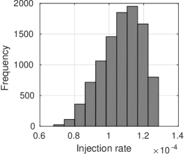
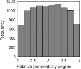
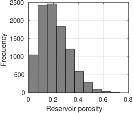
Figure 1: Parameter distributions of injection rate [m³/s], relative permeability degree [-] and reservoir porosity [-].

This study quantifies stochastic characteristics of the flow using mean value $\mu_{S_{g}}$ and standard deviation $\sigma_{S_{g}}$ of $\mathrm{CO}_{2}$ saturation as a function of space and time. Fig. 2 shows the statistical reference solution for the mean value and standard deviation of the $\mathrm{CO}_{2}$ saturation after $100$ days based on the set of samples $\Theta$. Apart from the global influence of the uncertain parameters onto the output statistics, Fig. 2 also illustrates the individual impact of each analyzed parameter. One can observe that the uncertainty in the degree of the relative permeability does not influence the dynamics of the saturation significantly. The injection rate and the reservoir porosity are the main cause of uncertainty in the $\mathrm{CO}_{2}$ saturation.

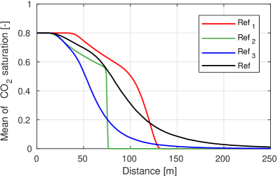
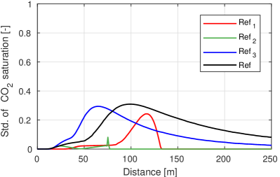
Figure 2: Mean and standard deviation of CO₂ saturation at $t=100$ days based on Monte Carlo sampling using $10^{4}$ samples: Ref₁ - uncertain injection rate; Ref₂ - uncertain relative permeability degree; Ref₃ - uncertain porosity; Ref - joint uncertainty.

4 Uncertainty quantification methods

In this section we briefly introduce four different methods for uncertainty quantification and discuss some of their properties. We compare them with the data-based statistics generated by Monte Carlo sampling for mean value and standard deviation of the quantity of interest (black line in Fig. 2).

4.1 Non-intrusive arbitrary polynomial chaos expansion

We briefly introduce arbitrary polynomial chaos (aPC) techniques that are employed to construct a global response surface which captures the dependence of the model on the data set. We consider space and time dependent model response $S(r,t;\boldsymbol{\theta})$ of the $\mathrm{CO}_{2}$ saturation. According to Wiener Wiener1938 the dependence of the model output on all input parameters is expressed via projection onto a multi-variate polynomial basis (see e.g. Ghanem_Spanos_1991_SFEM_book ), such that the model output $S$ can be approximated by the polynomial chaos expansion

$$S(r,t;\boldsymbol{\theta})\approx\sum_{i=0}^{N_{P}}S_{i}(r,t)\Phi_{i}(\boldsymbol{\theta}),$$ (16)

where $N_{P}$ is the number of multi-variate polynomial basis functions $\Phi_{i}(\boldsymbol{\theta})$ (see e.g. Ghanem_Spanos_1991_SFEM_book ) and corresponding coefficients $S_{i}(r,t)$. It depends on the total number of input parameters $M$ and on the order $N_{o}$ of the polynomial representation: $N_{P}=(M+N_{o})!/(M!N_{o}!)-1$. The coefficients $S_{i}(r,t)$ in equation (16) quantify the dependence of the model response $S(r,t;\boldsymbol{\theta})$ on the input parameters for each desired point in space $r$ and time $t$.

We follow a recent generalization of the polynomial chaos expansion known as the arbitrary polynomial chaos (aPC). The aPC technique adapts to arbitrary probability distribution shapes of the input parameters and can be inferred from limited data through a few statistical moments OladNowak_RESS2012 . The necessity to adapt to arbitrary distributions in practical tasks is discussed in more detail in OladNowak_AWR2010 . Thus, we explore a highly parsimonic and purely data-driven description of uncertainty via aPC and directly incorporate the available data set of size $10^{4}$ illustrated in Fig. 1 without any use of exact forms of probability density functions. For that, we compute $2N_{o}$ raw statistical moments from $10^{4}$ realisations and then we construct the orthonormal polynomial basis of order $N_{o}$ according to the matrix equation introduced in OladNowak_RESS2012 . Note that the orthonormal basis can be also obtained via recursive relations (see Chapter 22 of Abramowitz1965 ), via Gram-Schmidt orthogonalization (see Witteveen2007 ) or via the Stieltjes procedure Stieltjes1884 .

The polynomial representation in equation (16) is fully defined via the unknown expansion coefficients $S_{i}(r,t)$. These coefficients can be determined using intrusive or non-intrusive approaches. The intrusive approach requires manipulation of the governing equations and will be discussed in Section 4.4 via hybrid stochastic Galerkin. In the current Section 4.1 we follow the non-intrusive way where no modifications are required for the system of governing equations

As the computationally cheapest version we apply the non-intrusive probabilistic collocation method (PCM) Li2007 ; Olad_al_CG2009 . The method is based on a minimal chosen set of model evaluations, each with a defined set of model parameters (called collocation points) that is related to the roots of the polynomial basis via optimal integration theory Villadsen1978 . Fig. 3 shows mean and standard deviation of the CO₂ saturation estimated via aPC expansion based on the probabilistic collocation method and also shows the statistical reference solution. As expected, the strong discontinuity of the original physical model introduced due to the CO₂ displacement front poses challenges for the global polynomial representation. Nevertheless, the estimation of the mean value is acceptable. However, increasing the expansion order does not necessary lead to improvement of the results, especially for the variance estimation. Hence, a moderate expansion order can be seen as adequate compromise between accuracy and computational efforts. Additionally, the expansion order is only justified if accompanied by reliable statistical information, because incomplete statistical information limits the utility of polynomial chaos expansions oladyshkin2018incomplete .

As a computationally very demanding alternative to the probabilistic collocation method, we also employ the least-squares collocation method (e.g. Moritz1978 ) for constructing the expansion coefficients on a full tensor grid of collocation points. Fig. 3 also shows mean and standard deviation of CO₂ saturation estimated via aPC expansion based on the least-squares collocation method against the statistical reference solution. The least-squares collocation method based on the full tensor (FT) grid helps to overcome the typical oscillation problem of polynomials for high order expansions. However, due to the curse of dimensionality for tensor grids, this approach has an extremely high computational effort if more than a single parameter is of interest.

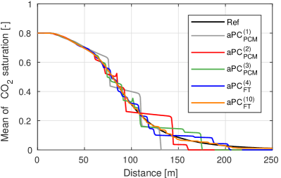
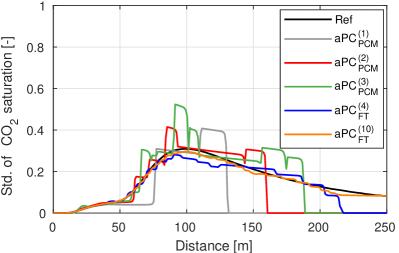
Figure 3: Mean and standard deviation of CO₂ saturation estimated via aPC expansion with probabilistic (PCM) and least-squares collocation method (FT): aPC${}^{(1)}_{PCM}$ - $1^{st}$ order expansion; aPC${}^{(2)}_{PCM}$ - $2^{nd}$ order expansion; aPC${}^{(3)}_{PCM}$ - $3^{rd}$ order expansion; aPC${}^{(4)}_{FT}$ - $4^{th}$ order expansion; aPC${}^{(10)}_{FT}$ - $10^{th}$ order expansion; Numbers in $(\cdot)$ indicate the number of model runs.

4.2 Spatially adaptive sparse grids

In this section we introduce regular sparse grids according to Zenger91Sparse . We follow the approach of higher-order basis functions that have been presented in Bungartz98Finite and extended in Pflueger10Spatially with proper extrapolation schemes. Furthermore, we present the concept of spatially adaptive refinement following Pflueger12Spatially and provide refinement criteria in the context of data-driven uncertainty quantification Franzelin15Non ; Ma09adaptive .

Let $\mathfrak{l}:=\{\mathfrak{l}_{1},\dots,\mathfrak{l}_{M}\}$ be a multi-index with $\mathfrak{l}_{j}>0$ and dimensionality $0<M$. We define a level-index set for some $\mathfrak{l}$ as

$$\mathcal{I}_{\mathfrak{l}}:=\{\mathfrak{i}\in{\mathbb{N}}^{M}\colon 1\leq\mathfrak{i}_{j}<2^{\mathfrak{l}_{j}},\mathfrak{i}_{j}\text{ odd},j=1,\dots,M\},$$ (17)

that defines grid points located at $\theta_{\mathfrak{l}_{j},\mathfrak{i}_{j}}:=2^{-\mathfrak{l}_{j}}\mathfrak{i}_{j}$. The multivariate basis functions are centered at the grid points and are defined as the tensor product of one-dimensional, local polynomials

$$\Phi_{\mathfrak{l},\mathfrak{i}}(\boldsymbol{\theta}):=\begin{cases}\prod_{j=1}^{M}\phi^{(\mathfrak{l}_{j}+1)}_{\mathfrak{l}_{j},\mathfrak{i}_{j}}(\theta_{j})&\text{for }\boldsymbol{\theta}\in X_{\mathfrak{l},\mathfrak{i}}\\ 0&\text{else}\;,\end{cases}$$ (18)

where $X_{\mathfrak{l},\mathfrak{i}}:=\bigtimes_{j=1,\dots,M}[2^{-\mathfrak{l}_{j}}(\mathfrak{i}_{j}-1),2^{-\mathfrak{l}_{j}}(\mathfrak{i}_{j}+1)]$ and $\mathfrak{l}_{j}+1$ is the polynomial degree in direction $j$.

Sparse grids use these functions to form a hierarchical basis in order to overcome the curse of dimensionality to some extent. The level-index sets $\mathcal{I}_{\mathfrak{l}}$ define a unique set of hierarchical increment spaces $W_{\mathfrak{l}}:=\textrm{span}\{\Phi_{\mathfrak{l},\mathfrak{i}}(\boldsymbol{\theta})\colon\mathfrak{i}\in\mathcal{I}_{\mathfrak{l}}\}$ that add the difference between the approximation on smaller levels (componentwise) and the actual level. Due to this hierarchical character, one can sort the increment spaces according to their benefit to the approximation of functions from various function spaces and leave out the less important ones. If the contribution of each $W_{\mathfrak{l}}$ to the approximation is measured with respect to the $L^{2}$-norm, then the optimal sparse grid level-index set is obtained as

$$\mathcal{I}_{\ell}:=\bigcup_{\mathfrak{l}\in{\mathbb{N}}^{M}\colon|\mathfrak{l}|_{1}\leq\ell+M-1}\{(\mathfrak{l},\mathfrak{i})\colon\mathfrak{i}\in\mathcal{I}_{\mathfrak{l}}\}\;,|\mathfrak{l}|_{1}:=\sum_{j=1}^{M}\mathfrak{l}_{j}\;,$$ (19)

with $\ell\in\mathbb{N}$ being the regular level of the grid. A regular sparse grid function $S_{\mathcal{I}_{\ell}}\in V_{\ell}:=\bigoplus_{|\mathfrak{l}|_{1}\leq\ell+M-1}W_{\mathfrak{l}}$ that approximates the model output $S$ is written as

$$S(r,t;\boldsymbol{\theta})\approx S_{\mathcal{I}_{\ell}}(r,t;\boldsymbol{\theta}):=\sum_{({\mathfrak{l},\mathfrak{i}})\in\mathcal{I}_{\ell}}v_{\mathfrak{l},\mathfrak{i}}(r,t)\Phi_{\mathfrak{l},\mathfrak{i}}(\boldsymbol{\theta})\;,$$ (20)

where the $v_{\mathfrak{l},\mathfrak{i}}(r,t)\in{\mathbb{R}}$ are called hierarchical coefficients.

The number of grid points $|\mathcal{I}_{\ell}|$ is significantly reduced compared to a full grid with the same spatial resolution in each direction. At the same time the interpolation error of a sparse grid differs just by a logarithmic factor compared to a full grid and is, hence, only slightly worse Bungartz98Finite ; Zenger91Sparse .

One can interpret such a regular sparse grid as the result of an a-priori adaptivity. Spatially adaptive sparse grids add a second level of refinement: Grid points are added iteratively where the local error of the approximation is largest. Refinement criteria estimate these local errors with respect to some target quantity. In this paper we use a weighted $L^{2}$-refinement method and enforce balancing Bungartz03Multivariate . It defines a ranking for all level-index pairs as

$$\max_{({\mathfrak{l},\mathfrak{i}})\in\mathcal{I}}\|S-S_{\mathcal{I}_{\ell}\setminus\{({\mathfrak{l},\mathfrak{i}})\}}\|_{L^{2}(\Omega)}\approx\max_{({\mathfrak{l},\mathfrak{i}})\in\mathcal{I}}|v_{\mathfrak{l},\mathfrak{i}}|\|\Phi_{\mathfrak{l},\mathfrak{i}}\|_{L^{2}(\Omega)}\;,$$ (21)

where $\mathcal{I}$ is an adaptive sparse grid index set. To refine, we add all the hierarchical successors of $({\mathfrak{l},\mathfrak{i}})\in\mathcal{I}$,

$$\{ ((\dots,\mathfrak{l}_{m}+1,\dots),(\dots,2\mathfrak{i}_{m}+1,\dots)),$$ (22)

$$((\dots,\mathfrak{l}_{m}+1,\dots),(\dots,2\mathfrak{i}_{m}-1,\dots))\}_{m=1}^{M}\;,$$

that are not yet part of $\mathcal{I}$ starting with the one that has the largest rank.

To describe the uncertainty, we use a sparse grid probability density function Franzelin16Data based on the input data to approximate $\|\Phi_{\mathfrak{l},\mathfrak{i}}\|_{L^{2}(\Omega)}$. This way, we can start with a purely data-driven description and arbitrary densities without any need for derived analytical forms or independence of the respective probability functions.

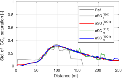
Figure 4: Mean and standard deviation of CO₂ saturation estimated via adaptive sparse grids with boundary points (aSG_b) and modified basis (aSG_m): aSG${}^{(101)}_{\textrm{b}}$ - after $3$ refinement steps; aSG${}^{(1021)}_{\textrm{b}}$ - after last refinement iteration; aSG${}^{(111)}_{\textrm{m}}$ - after $5$ refinement steps; aSG${}^{(1001)}_{\textrm{m}}$ - after last refinement iteration; Numbers in $(\cdot)$ indicate the number of model runs / grid points.

For this model problem we distinguish two types of sparse grids: The first model spends grid points directly at the boundary (Pflueger10Spatially, , p.15) to which we refer to as aSG_b. As a second model, we consider modified piecewise polynomial basis functions (Pflueger10Spatially, , p.24) with linear extrapolation, which we write as aSG_m. Both sparse grid surrogates are constructed as follows:

Step 1:

Start with a regular sparse grid $\mathcal{I}$ of $\ell=1$.

Step 2:

Compute the ranking (21) of all sparse grid points for which not all successors (22) exist. Add the successors of the two highest ranked level-index pairs to $\mathcal{I}$.

Step 3:

Make sure that all hierarchical ancestors of each grid point exist and that each grid point has either none or two hierarchical successors in each direction.

Step 4:

Run the model problem at the new grid points and construct the new interpolant.

Step 5:

Continue with step 2 until a maximum number of grid points is reached.

Sample results for the expectation value and the variance of the model problem are shown in Fig. 4. Both estimated quantities using a sparse grid with, for example, $101$ boundary points differ significantly from the statistical reference value. Most of the grid points are located at the boundary of the domain, which makes this approach unfeasible for problems with small computational budget. This problem can be solved with aSG_m . Hence, we observe a better approximation of the expectation value and the variance already for smaller grids. Nevertheless, the accuracy of the moments with respect to the reference solution increase with increasing grid size in both cases.

4.3 Kernel greedy interpolation

To start, we emphasize that we work here with the discretization of the saturation provided by the hyperbolic solver, thus we understand $S(r,t,\boldsymbol{\theta})$ as a function $X\to{\mathbb{R}}^{d}$, $X\subset{\mathbb{R}}^{3}$, $d:=250$, mapping the uncertain parameters to the spatial discretization consisting of 250 cells at final time. Kernel-based approximation methods construct a surrogate $S_{N}(\boldsymbol{\theta})$ of $S(r,t,\boldsymbol{\theta})$ based on a set $X_{N}\subset X$ of $N\in{\mathbb{N}}$ input parameters and the corresponding output computed by the solver. The surrogate model can then be rapidly evaluated on the large set $\Theta\subset X$ of input parameters of the reference solution, and the mean and variance are calculated as the mean and variance of these evaluations.

We give only a brief overview of kernel methods, and refer to Wendland2005 for a detailed treatment. The saturation is approximated as a vector-valued linear combination

$$S(r,t,\boldsymbol{\theta})\approx S_{N}(\boldsymbol{\theta}):=\sum\limits_{i=1}^{N}k(\boldsymbol{\theta},\boldsymbol{\theta}_{i})\boldsymbol{\alpha}_{i},\quad\boldsymbol{\theta}\in X,$$ (23)

where $k:X\times X\rightarrow{\mathbb{R}}$ is a symmetric kernel function, $\boldsymbol{\theta}_{i}\in X_{N}\subset X$ are the centers, and the coefficient vectors $\boldsymbol{\alpha}_{i}\in{\mathbb{R}}^{d}$ are determined by imposing interpolation conditions on $X_{N}$, i.e., (23) is exact when evaluated at $\boldsymbol{\theta}\in X_{N}$. These conditions result in a linear system, which has a unique solution whenever the kernel function is chosen to be strictly positive definite, i.e., for any choice of pairwise distinct points $X_{N}$ the matrix $K_{ij}:=k(\boldsymbol{\theta}_{i},\boldsymbol{\theta}_{j})$ is positive definite. Therefore, it is possible to construct an approximation (23) for arbitrary sample locations $X_{N}$ and input and output dimensions. In practice, orders of hundreds for input and output dimensions are realistic.

We use in the following a $C^{2}$ Wendland kernel Wendland1995a , which is a compactly supported radial kernel of polynomial type, and where the radius of the support is controlled by a shape parameter $\delta>0$. Each kernel is associated to a native Hilbert space $\mathcal{H}(X)$, which is in this case a Sobolev space.

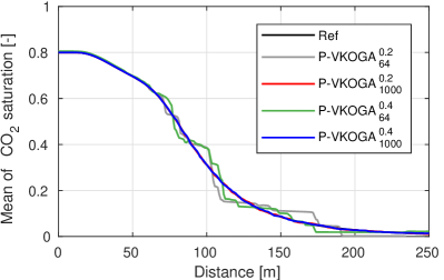
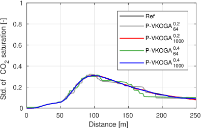
Figure 5: Mean and standard deviation of CO₂ saturation obtained via kernel interpolation with $P$-VKOGA${}_{n}^{\delta}$ for the shape parameters $\delta=0.2$, $\delta=0.4$, and number of model runs $n=64,1000$.

The quality of the kernel approximation in (23) depends on both the choice of $k$ and the set of centers $X_{N}$. Given a large set of possible sample locations $X_{N}$, we want to select of a subset $X_{n}\subset X_{N}$ such that the surrogate $S_{n}(\boldsymbol{\theta})$ based on $X_{n}$ is as good as $S_{N}(\boldsymbol{\theta})$, while ${n}\ll{N}$. This ensures that the evaluation of the approximation (23) is as fast as possible, so that it can be efficiently used in surrogate modeling.

For this, we apply $P$-VKOGA DeMarchi2005 ; Wirtz2013 (Vectorial Kernel Orthogonal Greedy Algorithm with $P$-greedy), to iteratively generate a nested sequence of centers $X_{n-1}\subset X_{n}\subset X_{N}$, $X_{0}:=\emptyset$. We give a rough outline for the motivation and structure of $P$-VKOGA and refer to the aforementioned references for further details: The interpolation error can be bounded by means of the power function $P_{X_{n}}:X\rightarrow[0,\infty)$ as

$$\|S(r,t,\boldsymbol{\theta})-S_{n}(\boldsymbol{\theta})\|_{\infty}\leq P_{X_{n}}(\boldsymbol{\theta})\|f\|_{\mathcal{H}(X)}\quad\forall\boldsymbol{\theta}\in X,$$ (24)

where the norm on the left-hand side is the maximal absolute value of all entries of the $d$-dimensional vector $S(r,t,\boldsymbol{\theta})-S_{n}(\boldsymbol{\theta})$. Observe that, when the kernel $k$ is understood as a covariance function, $P_{X_{n}}$ is precisely the expected prediction error of the corresponding simple Kriging, as discussed in scheuerer2013 .

Motivated by (24) we chose the centers iteratively by adding $\boldsymbol{\theta}^{\ast}=\arg\max\limits_{\boldsymbol{\theta}\in X_{N}\setminus X_{n}}P_{X_{n}}(\boldsymbol{\theta})$ to the previous set of centers, i.e. $X_{{n}+1}:=X_{{n}}\cup\{\boldsymbol{\theta}^{\ast}\}$. Using the Newton basis $\{v_{i}\}_{i=1}^{n}$ Muller2009 of the space $\textrm{span}(k(\cdot,\boldsymbol{\theta}_{i}),\boldsymbol{\theta}_{i}\in X_{n})$, the power function can be efficiently updated via $P_{X_{n}}(\boldsymbol{\theta})^{2}=k(\boldsymbol{\theta},\boldsymbol{\theta})-\sum\limits_{i=1}^{n}v_{i}(\boldsymbol{\theta})^{2}.$ Once a sufficient set $X_{n}$ is generated, the coefficients $\boldsymbol{\alpha}_{i}\in{\mathbb{R}}^{d}$ can be computed by solving the system (23) with interpolation conditions restricted to the points $X_{n}$. This method requires only the knowledge of a sampling $X_{N}$ of the input space $X$ to select the few sampling points $X_{n}$, and the solver is run only on the parameters in $X_{n}$. We remark that it has been recently proven that $P$-VKOGA, although simple, has a quasi-optimal convergence order in Sobolev spaces SH16b , i.e., it gives the same approximation order of full interpolation.

In the present setting, the surrogate model is constructed on the set $X$ defined as the convex hull of the reference data points $\Theta$. We run $P$-VKOGA starting from a fine discretization $X_{N}$ of $X$ obtained by intersecting $X$ with a uniform grid of $50\times 50\times 50$ equally spaced points in the minimum box enclosing $\Theta$. The resulting set $X_{N}$ contains $N=86021$ data points. We remark again that this set is used to perform the greedy optimization, and no function evaluation (i.e., no model run) on $X_{N}$ is needed at this stage. Since in this setting the number of model runs is the crucial computational constraint, we avoid to select the kernel width parameter $\delta$ via validation, and instead train different models for values $\delta=0.1,0.2,0.3,0.4,0.5$.

Each run of the algorithm selects incremental sets $X_{n}$ of point locations, and for each of the $5$ parameters $\delta$ we consider $6$ log-spaced values of $n$ in $[1,1000]$, i.e., $n=1,4,16,64,252,1000$. On these sets $X_{n}$ of input parameters, the full model is evaluated and for each of them the interpolant is computed. The resulting $30$ different models are denoted as $P$-VKOGA${}_{n}^{\delta}$, where the lower index is the number of model runs and the upper one is the kernel shape parameter. Sample results are shown in Fig. 5 for values $\delta=0.2,0.4$ and for an increasing number $n$. Although the surrogates are not accurate when using only $n=4$ model runs, it is evident that an increase in $n$ leads to a satisfactory convergence of the approximate mean and standard deviation to the reference ones. Indeed, the surrogates obtained with $64$ model runs are close enough to the reference solution, with some oscillations around the exact values. For $1000$ runs, the reference and the surrogates are almost equal. A more quantitative error analysis is discussed in the next sections.

4.4 Hybrid stochastic Galerkin

Contrary to the previous methods, the hybrid stochastic Galerkin (HSG) approach is an intrusive method which changes the deterministic system by means of the polynomial chaos expansion and a multi-element decomposition of the stochastic space, hence, does not construct a surrogate. We briefly summarize the discretization following Buerger2012 ; Koeppel2017 . For the sake of brevity we again use $S:=S_{g}^{\ast}$.

If all sources of uncertainty are considered, c.f. Section 3, the radial transport equation (11) yields the following randomized partial differential equation

$$\phi(\boldsymbol{\theta})\frac{\partial S(\boldsymbol{\theta})}{\partial t}-\frac{1}{r}\frac{\partial}{\partial r}\big{(}Q(\boldsymbol{\theta})f_{g}(S,\boldsymbol{\theta})\big{)}-q_{\mathrm{CO}_{2}}=0.$$ (25)

For the multi-element discretization we decompose the stochastic domain into $2^{MN_{r}}$ stochastic elements with refinement level $N_{r}\in{\mathbb{N}}_{0}$. For reasons of readability we describe the discretization based on the domain $[0,1]^{M}$. By rescaling, the method can be easily extended to arbitrary domains. Let $\tilde{\mathcal{I}}:=\{0,1,\ldots,2^{N_{r}}-1\}$ be a set of indices and $\mathcal{I}:=\tilde{\mathcal{I}}^{M}$ with multi-index $\mathfrak{l}=(\mathfrak{l}_{1},\ldots,\mathfrak{l}_{M})\in\mathcal{I}$. Then we define the $M$-dimensional stochastic element $\mathsf{I}^{N_{r}}_{M,\mathfrak{l}}:=\mathsf{I}^{N_{r}}_{\mathfrak{l}_{1}}\,\times\ldots\times\,\mathsf{I}^{N_{r}}_{\mathfrak{l}_{M}}$ with support $\mathsf{I}^{N_{r}}_{\mathfrak{l}_{i}}:=[2^{-N_{r}}\mathfrak{l}_{i},\,2^{-N_{r}}(\mathfrak{l}_{i}+1)]$, for $\mathfrak{l}_{i}\in\tilde{\mathcal{I}}$, $i\,=\,1,\dots,M$. Furthermore let $\mathcal{X}^{N_{o},\,N_{r}}_{M}$ be the space of piecewise polynomial functions on each stochastic element $\mathsf{I}^{N_{r}}_{M,\mathfrak{l}}$ with maximal polynomial order $N_{o}$. The space $\mathcal{X}^{N_{o},\,N_{r}}_{M}$ is spanned by the multivariate polynomials

$$\Phi_{\mathfrak{p},\mathfrak{l}}^{N_{r}}(\boldsymbol{\theta}):=\begin{cases}2^{MN_{r}/2}\prod_{k=1}^{M}\varphi_{\mathfrak{p}_{k}}(2^{N_{r}}\theta_{k}-\mathfrak{l}_{k}),&\mbox{for}\;\boldsymbol{\theta}\in\mathsf{I}^{N_{r}}_{M,\mathfrak{l}},\\ 0,&\text{otherwise},\end{cases}$$

with $\mathfrak{p}:=(\mathfrak{p}_{1},\ldots,\mathfrak{p}_{M})\in{\mathbb{N}}_{0}^{M},\;\left|\mathfrak{p}\right|\leq N_{o}$, $\mathfrak{l}\in\mathcal{I}$, and the truncated polynomial chaos polynomials $\varphi_{\mathfrak{p}_{k}}(\theta_{k})$. For the latter we use Legendre polynomials. The polynomials $\Phi_{\mathfrak{p},\mathfrak{l}}^{N_{r}}(\boldsymbol{\theta})$ satisfy the following orthonormality relation $\left\langle\Phi_{\mathfrak{p},\mathfrak{l}}^{N_{r}},\,\Phi_{\mathfrak{q},\mathfrak{m}}^{N_{r}}\right\rangle_{L^{2}(\Omega)}:=\delta_{\mathfrak{p},\mathfrak{q}}\delta_{\mathfrak{l},\mathfrak{m}},$where $\delta_{\mathfrak{p},\mathfrak{q}},\,\delta_{\mathfrak{l},\mathfrak{m}}$ denote the Kronecker delta symbol for $\mathfrak{p},\mathfrak{q}\in{\mathbb{N}}_{0}^{M},\;\left|\mathfrak{p}\right|,\left|\mathfrak{q}\right|\leq N_{o}$, and $\mathfrak{l},\mathfrak{m}\in\mathcal{I}$. The finite number of basis functions is given by $\tilde{P}:=2^{MN_{r}}(N_{o}+M)!/(N_{o}!M!)$. Based on these considerations the projection of a random field $S(r,t,\boldsymbol{\theta})$, $(r,t)\in D_{T}$ is obtained by

$$S(r,t,\boldsymbol{\theta})\approx\,\Pi^{{N_{r}},{N_{o}}}\left[{S}\right](r,t,\boldsymbol{\theta})\\ :=\sum_{\mathfrak{l}\in\mathcal{I}}\sum_{p=0}^{N_{o}}\sum_{\left|\mathfrak{p}\right|=p}{S}^{N_{r}}_{\mathfrak{p},\mathfrak{l}}(r,t)\Phi_{\mathfrak{p},\mathfrak{l}}^{N_{r}}(\boldsymbol{\theta}),\qquad$$ (26)

with deterministic coefficients ${S}^{N_{r}}_{\mathfrak{p},\mathfrak{l}}:=\left\langle S,\,\Phi_{\mathfrak{p},\mathfrak{l}}^{N_{r}}\right\rangle_{L^{2}(\Omega)}$, for $0\leq\left|\mathfrak{p}\right|\leq N_{o}$ and $\mathfrak{l}\in\mathcal{I}$. We note that without the multi-element decomposition the expansion (26) would be similar to (16). For more details concerning the convergence of $\Pi^{{N_{r}},{N_{o}}}\left[{S}\right]$ for $N_{o},\,N_{r}\to\infty$, we refer to MR1199538 . Moreover, we refer to Buerger2012 ; Koeppel2017 for a more detailed description of the HSG method.

We apply the stochastic discretization to (25) by replacing the unknown random field, i.e. the saturation $S(x,t,\boldsymbol{\theta})$, with its HSG projection $\Pi^{{N_{r}},{N_{o}}}\left[{S}\right]$ and by testing the equation with the HSG basis functions $\Phi_{\mathfrak{p},\mathfrak{l}}^{N_{r}}$. Then we obtain a partly decoupled system for the deterministic coefficients ${S}^{N_{r}}_{\mathfrak{p},\mathfrak{l}}$ which reads

$$\partial_{t}{S}^{N_{r}}_{\mathfrak{p},\mathfrak{l}}+(1/r)\;\mathrm{div}\left\langle Qf_{g}\big{(}\Pi^{{N_{r}},{N_{o}}}\left[{S}\right]\big{)}/\phi,\,\Phi_{\mathfrak{p},\mathfrak{l}}^{N_{r}}\right\rangle_{L^{2}(\Omega)}\\ -\left\langle q_{\mathrm{CO}_{2}}/\phi,\,\Phi_{\mathfrak{p},\mathfrak{l}}^{N_{r}}\right\rangle_{L^{2}(\Omega)}=0,\quad$$ (27)

with initial values ${S}^{N_{r}}_{\mathfrak{p},\mathfrak{l}}(\cdot,0)=\left\langle S_{0},\,\Phi_{\mathfrak{p},\mathfrak{l}}^{N_{r}}\right\rangle_{L^{2}(\Omega)}$. On $\partial D$ we impose deterministic boundary conditions.

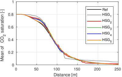
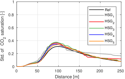
Figure 6: Mean and standard deviation of CO₂ saturation obtained via reconstruction of HSG discretization wihtout and with decomposed stochastic space. HSG₁: $N_{r}=2$, $N_{o}=1$. HSG₂: $N_{r}=3$, $N_{o}=1$. HSG₃: $N_{r}=2$, $N_{o}=2$, and $N_{r}=3$, $N_{o}=3$. HSG₄: $N_{r}=3$, $N_{o}=1$, and $N_{r}=3$, $N_{o}=1$. HSG₅: $N_{r}=3$, $N_{o}=1$, and $N_{r}=4$, $N_{o}=1$.

Mean and standard deviation are then computed during the post-processing. In contrast to the common SG/HSG ansatz, in this work the simulations are performed with Legendre polynomials representing a uniform distribution even if the actual distribution might be different. In view of data-driven UQ this guarantees that every point is uniformly approximated. Instead of using the coefficients of (26) directly mean and standard deviation are obtained by a reconstruction using the parameters provided in the data set $\Theta$. This is possible since equation (26) allows to compute the approximation of the unknown random field for an arbitrary parameter set. However this approach is likely to be at the expense of the accuracy. On the other hand we obtain mean and standard deviation for arbitrary input data without a rerun of the simulation.

Fig. 6 shows the results of the HSG method compared with the reference solution. An increase of $N_{r}$ leads to a greater improvement of the results than an increase of $N_{o}$ only. Since in the test case the value of the perturbed porosity $\phi$ has a significant influence on the dynamics of the system, some of the shown simulations are decoupled in two parts w.r.t. the value of $\phi$. By merging the decoupled results during the post-processing the accuracy can be improved. Even though the time steps on different stochastic elements differ from each other, the time step size on each stochastic element of the considered problem does not change during the whole computation time. Therefore, we improved the computational efficiency significantly by rearranging the stochastic elements on several Message Passing Interface (MPI) ranks in terms of the expected number of time steps.

5 Discussion

This section discusses the results obtained by the four different methods in more detail and compares them with respect to five different criteria. The results are visualized in Fig. 7 to facilitate the reading. Moreover we report in Table 2 a summary of the discussion to provide the reader with an immediate comparison of the strengths and weaknesses of the different techniques. However we emphasize that the comparison needs to be evaluated with caution due to the inherent differences of the methods.

5.1 Usage for UQ in geosciences

The polynomial chaos expansion is a known technique in the field of uncertainty quantification and its generalization to arbitrary distributions has been applied already to CO₂ storage problems. Similarly, spatially adaptive sparse grids are a common stochastic collocation method in uncertainty quantification that has been applied to a large variety of real-world problems. Kernel-based methods are successfully applied in a variety of data-based tasks, in particular in function approximation, but still novel in uncertainty quantification in geosciences. The use of kernel models in the context of uncertainty quantification in principle poses no particular issues, as the mean and variance predictions can be simply obtained by evaluating the surrogate model and computing the corresponding empirical mean and variance.

By construction, intrusive stochastic Galerkin methods change the structure of the problem. Consequently, the quantification of uncertainties goes along with the underlying deterministic problem to be solved. In the early 90’s, intrusive stochastic Galerkin methods have been successfully used for the quantification of uncertainties of elliptic problems, e.g. by Ghanem and Spanos Ghanem_Spanos_1991_SFEM_book . In the last decades these methods have been extended further to cope with several applications of different complexity. In particular, nonlinear hyperbolic problems require an additional stochastic discretization, such as the multi-wavelet approach or the HSG method, involving the decomposition of the stochastic space in order to avoid or reduce the generally occurring Gibbs phenomenon.

5.2 Comput. costs to evaluate & reconstruct surrogate

Polynomial chaos expansions and its recent data-driven aPC generalization can be seen as a cheap way for the estimation of uncertainty. Therefore the computational costs involved are comparatively low.

Due to its nature, the same applies to sparse grid methods. All sparse grid methods used in this paper are publicly available in SG⁺⁺ Pflueger10Spatially . This toolbox includes state-of-the-art sparse-grid algorithms that allow for very efficient and parallel construction, evaluation and quadrature of sparse grid surrogates.

Greedy methods prove to be particularly effective in general surrogate modeling since they produce sparse, hence cheap-to-evaluate models. This is the case also in the present setting, while greedy data-independent methods, as the presently used $P$-greedy algorithm, have the further advantage of not requiring an a-priori knowledge of the full model evaluations. Indeed, one of the measures for the success of a method is the number of model runs required to construct the surrogate.

The results of the HSG method with low resolution can be computed with appropriate computational effort, but the complexity of the problem and also the computational costs increase rapidly with increasing resolution. However, the method facilitates a change of the probability distribution provided that it is still defined on the same interval, almost without any computational costs during the postprocessing. Furthermore the partially decoupled structure of the HSG-discretized problem allows for efficient parallelization on MPI and Open Multi-Processing clusters. Additional improvements of the computational efficiency can be achieved by the stochastic adaptivity Barth201611 ; Buerger2012 and load balancing based on the stochastic elements. It is also promising to exploit the vector structure of the discretization by using GPU-based architectures.

5.3 Accuracy for low number of model runs/resolution

Low-order aPC representations such as 1^st and 2^nd order seem to be efficient in terms of computational costs and corresponding accuracy (see Fig. 7). However, the aPC approach covers the parameter space globally and as a consequence has not enough flexibility to represent special features in parameter space such as strong discontinuities, shocks, etc.

As shown in Fig. 7, sparse grids are efficient with respect to accuracy and the corresponding computational costs. For a very limited computational budget with less than $20$ model runs, the convergence of the sparse grid with the modified basis is limited by the grid structure from which the interpolation points are taken.

The results of the $P$-greedy method show that a certain minimal number of data is required to have meaningful predictions (at least $50$ model runs). This is motivated by two factors: first, the model does not incorporate any knowledge on the input space distribution. Second, the $P$-greedy algorithm selects the input points in a target-function-independent way, so it is not specialized on the approximation of this specific model.

The HSG method provides suitable accuracy for low resolutions of mean and standard deviation, cf. Fig. 7. This applies in particular to the bisection level $N_{r}$, i.e. the number of stochastic elements. The choice of the polynomial order $N_{o}$ has no significant bearing on the accuracy of the considered problem.

5.4 Accuracy for high numb. of model runs/resolution

As pointed out in Section 4.1, an increase of the expansion order in aPC does not necessarily lead to an improvement. This fact is very well illustrated in Fig. 7. Apparently the 0^th order estimation of the standard deviation which suggests by definition a value of $0$ and demands one run of the original model only, is more accurate than the 5^th order expansion. Alternatively, this artifact can be mitigated via least-squares projection onto the full tensor grid, as presented in Fig. 7. The aPC based on least-squares collocation helps to overcome the problem of representing discontinuities and assures the reduction of the error. However this is at the expense of the computational costs involved.

The efficiency of the sparse grids method with modified basis increases significantly when the adaptive refinement comes into play, as both the level of the grid and the accuracy of the surrogate increase in the regions of high probability. The error keeps converging as expected with an increasing number of model runs. Sparse grids with boundary points converge as well, however with higher computational costs (see Fig. 7). Consequently, they should not be considered for data-driven uncertainty quantification problems in higher dimensions or with small computational budgets.

The results and comparisons of Fig. 7 demonstrate a good behavior of the $P$-greedy algorithm in the present task and, in particular, suitable numerical convergence as the size of the dataset increases. This behavior is particularly evident for larger datasets (i.e. when at least $50$ model runs are utilized), as the surrogate model improves its accuracy, which turns out to be an advantage over other methods.

The HSG method provides fair accuracy for high resolutions of mean and standard deviation for increasing $N_{r}$ and $N_{o}$. An increase of the bisection level $N_{r}$ usually leads to higher accuracy than the increase of the highest polynomial order $N_{o}$, cf. Fig. 7. Because of the considered setup, numerical quadrature needs to be performed in each time step. Depending on the desired accuracy, the discretization of the setup includes up to several hundreds of thousands time steps. This may result in numerical difficulties and also accuracy limitations.

5.5 Applicability for large number of parameters

In general, the different aPC approaches used in this work are not very suitable for high-dimensional problems due to the curse of dimensionality. Only an extension to sparse polynomial representation can be feasible for applied tasks ahlfeld2016samba .

In contrast, spatially adaptive sparse grids have three main advantages compared to the other approaches. First, as pointed out in Section 4.2, they are suited for higher-dimensional problems. Second, they adaptively allow to change the approximation locally wherever local features in the parameter space appear. Large hierarchical coefficients describe large local changes and, hence, serve as a basis for refinement criteria. It is even possible to cope with functions that include kinks or jumps. And third, they are very flexible and allow $p$-adaptive refinement. This means one can choose the polynomial degree of each basis function separately in order to exploit local smoothness of the model function.

The $P$-greedy method can potentially work on problems with many more input dimensions, although a slower convergence rate should be expected due to the curse of dimensionality. Nevertheless, the complexity of the model construction and evaluation remain essentially the same, up to the computation of Euclidean distances between points in a larger input space.

As mentioned, all intrusive techniques base on a transformation of the randomized problem into a deterministic system of equations and, at least in the general case, they require the application of a quadrature in each time step. Compared to non-intrusive methods this methodology therefore changes the structure of the problem. Consequently, intrusive methods including HSG suffer from the curse of the dimensionality.

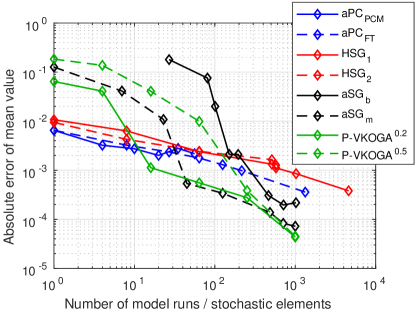
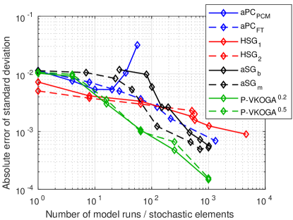
Figure 7: Absolute error of mean and standard deviation versus the number of model runs / stochastic elements (cf. HSG): aPC_PCM - aPC expansion based on the probabilistic collocation method; aPC_FT - aPC expansion based on the least-squares collocation method; HSG₁ - HSG method with maximal polynomial order $N_{o}=1$; HSG₂ - HSG method with maximal polynomial order $N_{o}=2$; aSG_b - adaptive sparse grids with boundary points; aSG_m - adaptive sparse grids without boundary points but with a modified basis; $P$-VKOGA^δ - kernel greedy interpolation with shape parameter $\delta=0.2,0.5$.

	Usage in geoscience UQ	Comput. costs to reconstruct & evaluate surrogate	Accuracy for low number of model runs/resolution	Accuracy for high number of model runs/resolution	High-dimensional applicability
aPCPCM	Very common	Suitable	Suitable	Not Suitable	Not Suitable
aPCFT	Common	Suitable	Suitable	Acceptable	Not Suitable
aSG	Common	Suitable	Acceptable	Acceptable	Acceptable
$P$-VKOGA	Uncommon	Suitable	Acceptable	Suitable	Acceptable
HSG	Very common	Acceptable	Suitable	Acceptable	Not Suitable

Table 2: Comparison of the methods w.r.t. the five criteria of Section 5. The different colors reflect the behavior of the methods

6 Summary and Conclusions

In this benchmark study we have compared four promising techniques for data-driven uncertainty quantification of nonlinear two-phase flow in porous media. The flow problem is motivated by an injection scenario of supercritical $\mathrm{CO}_{2}$ into a porous and saline aquifer where the consideration of uncertainty in the boundary conditions, uncertainty in material parameters as well as conceptual model uncertainty has a significant bearing on the overall flow and storage behavior of the system. Therefore, we have considered uncertainty in the injection rate related to boundary value uncertainty, uncertain porosity related to the limited data availablity of field-scale storage sites and uncertainty of the relative permeability degree associated with the nonlinearity of the conceptual model. To account for the arising uncertainties, we considered the non-intrusive methods arbitrary polynomial chaos, spatially adaptive sparse grids and kernel greedy interpolation as well as the intrusive hybrid stochastic Galerkin method. They were compared by means of the absolute error of the moments mean and standard deviation of the $\mathrm{CO}_{2}$ saturation after 100 days based on a statistical reference solution.

The numerical results show that all methods provide a good representation of the considered moments of the quantity of interest, despite the inherent complexity stemming from the distribution and the impact of the uncertain parameters. Small changes of these parameters may strongly influence the nonlinearity of the flow problem and may cause large variability of the simulation time of the hyperbolic solver resulting in significant changes of the $\mathrm{CO}_{2}$ saturation and the shape of the plume. This usually leads to Gibbs phenomena and oscillations of response surfaces in UQ methods. The arbitary polynomial chaos method and the hybrid stochastic Galerkin method overcome these difficulties already for low number of model runs/resolution, whereas adaptive sparse grids and the kernel greedy method are characterized by improved accuracy at higher number of model runs/resolution. The applicability to high dimensionalities needs to be taken into account. Our discussion indicates that the arbitary polynomial chaos method and the hybrid stochastic Galerkin method are generally less efficient and typically suffer more from the curse of dimensionality compared to adaptive sparse grids and the kernel greedy interpolation technique. The particular method of choice therefore depends on the specific problem and specific goal to be achieved. Taking this fact into consideration we have classified the methods regarding five relevant properties which are presented in Table 2. The classification reflects the main features we deem to be useful for further uncertainty quantification for $\mathrm{CO}_{2}$ storage and beyond.

The authors would like to thank the German Research Foundation (DFG) for financial support of the project within the Cluster of Excellence in Simulation Technology (EXC 310/2) at the University of Stuttgart.

References

- (1) Abramowitz, M., Stegun, I.A.: Handbook of Mathematical Functions with Formulas, Graphs, and Mathematical Tables. New York: Dover (1965)
- (2) Ahlfeld, R., Belkouchi, B., Montomoli, F.: SAMBA: sparse approximation of moment-based arbitrary polynomial chaos. J. Comput. Phys. 320, 1–16 (2016)
- (3) Alkhateeb, O., Ida, N.: Data-Driven Multi-Element Arbitrary Polynomial Chaos for Uncertainty Quantification in Sensors. IEEE Trans. Magn. (2017)
- (4) Alpert, B.K.: A class of bases in for the sparse representation of integral operators. SIAM J. Math. Anal. 24(1), 246–262 (1993)
- (5) Barth, A., Bürger, R., Kröker, I., Rohde, C.: Computational uncertainty quantification for a clarifier-thickener model with several random perturbations: A hybrid stochastic Galerkin approach. Comput. Chem. Eng. 89, 11 – 26 (2016)
- (6) Birkholzer, J.T., Zhou, Q., Tsang, C.F.: Large-scale impact of CO2 storage in deep saline aquifers: A sensitivity study on pressure response in stratified systems. Int. J. Greenh. Gas Control 3, 181–194 (2009)
- (7) Blatman, G., Sudret, B.: Sparse polynomial chaos expansions and adaptive stochastic finite elements using a regression approach. C. R. Mécanique 336(6), 518–523 (2008)
- (8) Bungartz, H.J.: Finite Elements of Higher Order on Sparse Grids. Habilitation, Technische Universität München (1998)
- (9) Bungartz, H.J., Dirnstorfer, S.: Multivariate Quadrature on Adaptive Sparse Grids. Computing 71(1), 89–114 (2003)
- (10) Bürger, R., Kröker, I., Rohde, C.: A hybrid stochastic Galerkin method for uncertainty quantification applied to a conservation law modelling a clarifier-thickener unit. ZAMM Z. Angew. Math. Mech. 77(10), 793–817 (2014)
- (11) Celia, M., Bachu, S., Nordbotten, J., Bandilla, K.: Status of CO2 storage in deep saline aquifers with emphasis on modeling approaches and practical simulations. Water Resour. Res. 51(9), 6846–6892 (2015)
- (12) Class, H., Ebigbo, A., Helmig, R., Dahle, H., Nordbotten, J.N., Celia, M.A., Audigane, P., Darcis, M., Ennis-King, J., Fan, Y., Flemisch, B., Gasda, S., Jin, M., Krug, S., Labregere, D., Naderi, A., Pawar, R.J., Sbai, A., Sunil, G.T., Trenty, L., Wei, L.: Abenchmark-study on problems related to CO2 storage in geologic formations. Comput. Geosci. 13, 451֭467 (2009)
- (13) Court, B., Bandilla, K.W., Celia, M.A., Janzen, A., Dobossy, M., Nordbotten, J.M.: Applicability of vertical-equilibrium and sharp-interface assumptions in CO2 sequestration modeling. Int. J. Greenh. Gas Control 10, 134–147 (2012)
- (14) De Marchi, S., Schaback, R., Wendland, H.: Near-optimal data-independent point locations for radial basis function interpolation. Adv. Comput. Math. 23(3), 317–330 (2005)
- (15) Ebigbo, A., Class, H., Helmig, R.: CO2 leakage through an abandoned well: problem-oriented benchmarks. Comput. Geosci. 11(2), 103–115 (2007)
- (16) Elsheikh, A.H., Hoteit, I., Wheeler, M.F.: Efficient Bayesian inference of subsurface flow models using nested sampling and sparse polynomial chaos surrogates. Comput. Methods in Appl. Mech. Eng. 269, 515–537 (2014)
- (17) Foo, J., Karniadakis, G.: Multi-element probabilistic collocation method in high dimensions. J. Comput. Phys. 229(5), 1536–1557 (2010)
- (18) Franzelin, F., Diehl, P., Pflüger, D.: Non-intrusive Uncertainty Quantification with Sparse Grids for Multivariate Peridynamic Simulations. In: M. Griebel, M.A. Schweitzer (eds.) Meshfree Methods for Partial Differential Equations VII, Lecture Notes in Computational Science and Engineering, vol. 100, pp. 115–143. Springer International Publishing (2015)
- (19) Franzelin, F., Pflüger, D.: From Data to Uncertainty: An Efficient Integrated Data-Driven Sparse Grid Approach to Propagate Uncertainty, pp. 29–49. Springer International Publishing, Cham (2016)
- (20) Ghanem, R.G., Spanos, P.D.: Stochastic finite elements: A spectral approach. Springer-Verlag, New York (1991)
- (21) Hansson, A., Bryngelsson, M.: Expert opinions on carbon dioxide capture and storage: A framing of uncertainties and possibilities. Energy Policy 37, 2273–2282 (2009)
- (22) Helton, J., Davis, F.: Latin hypercube sampling and the propagation of uncertainty in analyses of complex systems. Reliab. Eng. Syst. Saf. 81(1), 23–69 (2003)
- (23) IPCC: Special report on carbon dioxide capture and storage, Technical report, Intergovernmental Panel on Climate Change (IPCC), prepared by Working Group III. Cambridge University Press, Cambridge, United Kingdom and New York, NY, USA (2005)
- (24) Isukapalli, S.S., Roy, A., Georgopoulos, P.G.: Stochastic Response Surface Methods (SRSMs) for uncertainty propagation: Application to environmental and biological systems. Risk Anal. 18(3), 351–363 (1998)
- (25) Jakeman, J.D., Archibald, R., Xiu, D.: Characterization of discontinuities in high-dimensional stochastic problems on adaptive sparse grids. J. Comput. Phys. 230(10), 3977–3997 (2011)
- (26) Keese, A., Matthies, H.G.: Sparse quadrature as an alternative to Monte Carlo for stochastic finite element techniques. Proc. Appl. Math. Mech. 3, 493֭494 (2003)
- (27) Kopp, A., Class, H., Helmig, H.: Investigations on CO2 Storage Capacity in Saline Aquifers - Part 1: Dimensional Analysis of Flow Processes and Reservoir Characteristics. Int. J. Greenh. Gas Control 3, 263–276 (2009)
- (28) Köppel, M., Franzelin, F., Kröker, I., Oladyshkin, S., Santin, G., Wittwar, D., Barth, A., Haasdonk, B., Nowak, W., Pflüger, D., Rohde, C.: Datasets and executables of data-driven uncertainty quantification benchmark in carbon dioxide storage 10.5281/zenodo.933827
- (29) Köppel, M., Kröker, I., Rohde, C.: Intrusive uncertainty quantification for hyperbolic-elliptic systems governing two-phase flow in heterogeneous porous media. Comput. Geosci. 21(4), 807–832 (2017)
- (30) Kröker, I., Nowak, W., Rohde, C.: A stochastically and spatially adaptive parallel scheme for uncertain and nonlinear two-phase flow problems. Comput. Geosci. pp. 1–16 (2015)
- (31) Kurganov, A., Petrova, G.: Central-upwind schemes on triangular grids for hyperbolic systems of conservation laws. Numer. Meth. Part. D. E. 21(3), 536–552 (2005)
- (32) LeVeque, R.: Numerical Methods for Conservation Laws. Lectures in Mathematics ETH Zürich. Springer (1992)
- (33) Li, H., Zhang, D.: Probabilistic collocation method for flow in porous media: Comparisons with other stochastic methods. Water Resour. Res. 43, 44–48 (2007)
- (34) Lin, G., Tartakovsky, A.: An efficient, high-order probabilistic collocation method on sparse grids for three-dimensional flow and solute transport in randomly heterogeneous porous media. Adv. Water Res. 32(5), 712–722 (2009)
- (35) Ma, X., Zabaras, N.: An adaptive hierarchical sparse grid collocation algorithm for the solution of stochastic differential equations. J. Comput. Phys. 228(8), 3084–3113 (2009)
- (36) Matthies, H.G., Keese., A.: Galerkin methods for linear and nonlinear elliptic stochastic partial differential equations. Comp. Meth. Appl. Mech. Engrg. 194, 1295–1331 (2005)
- (37) Moritz, H.: Least-Squares Collocation. Rev. Geophys. 16(3), 421–430 (1978)
- (38) Müller, S., Schaback, R.: A Newton basis for kernel spaces. J. Approx. Theory 161(2), 645–655 (2009)
- (39) Namhata, A., Oladyshkin, S., Dilmore, R.M., Zhang, L., Nakles, D.V.: Probabilistic Assessment of Above Zone Pressure Predictions at a Geologic Carbon Storage Site. Scientific reports 6, 39,536 (2016)
- (40) Nordbotten, J., Celia, M., Bachu, M.: Injection and storage of CO2 in deep saline aquifers: analytical solution for CO2 plume evolution during injection. Transport Porous Med. 58(3), 339–360 (2005)
- (41) Nordbotten, J.M., Dahle, H.K.: Impact of the capillary fringe in vertically integrated models for CO2 storage. Water Resour. Res. 47(2) (2011). W02537
- (42) Oladyshkin, S., Class, H., Helmig, R., Nowak, W.: A concept for data-driven uncertainty quantification and its application to carbon dioxide storage in geological formations. Adv. Water Res. 34, 1508–1518 (2011)
- (43) Oladyshkin, S., Class, H., Helmig, R., Nowak, W.: An integrative approach to robust design and probabilistic risk assessment for CO2 storage in geological formations. Comput. Geosci. 15(3), 565–577 (2011)
- (44) Oladyshkin, S., Class, H., Nowak, W.: Bayesian updating via Bootstrap filtering combined with data-driven polynomial chaos expansions: methodology and application to history matching for carbon dioxide storage in geological formations. Comput. Geosci. 17(4), 671–687 (2013)
- (45) Oladyshkin, S., Nowak, W.: Data-driven uncertainty quantification using the arbitrary polynomial chaos expansion. Reliab. Eng. Syst. Safe. 106, 179–190 (2012)
- (46) Oladyshkin, S., Nowak, W.: Incomplete statistical information limits the utility of high-order polynomial chaos expansions. Reliability Engineering & System Safety 169, 137–148 (2018)
- (47) Oladyshkin, S., Schroeder, P., Class, H., Nowak, W.: Chaos expansion based Bootstrap filter to calibrate CO2 injection models. Energy Procedia 40, 398–407 (2013)
- (48) Peherstorfer, B.: Model Order Reduction of Parametrized Systems with Sparse Grid Learning Techniques. Ph.D. thesis, Technical University of Munich (2013)
- (49) Pettersson, P., Tchelepi, H.A.: Stochastic Galerkin framework with locally reduced bases for nonlinear two-phase transport in heterogeneous formations. Comput. Method. Appl. Mech. Eng. 310, 367 – 387 (2016)
- (50) Pfander, D., Heinecke, A., Pflüger, D.: A New Subspace-Based Algorithm for Efficient Spatially Adaptive Sparse Grid Regression, Classification and Multi-evaluation. In: J. Garcke, D. Pflüger (eds.) Sparse Grids and Applications - Stuttgart 2014, pp. 221–246. Springer International Publishing (2016)
- (51) Pflüger, D.: Spatially Adaptive Sparse Grids for High-Dimensional Problems. Verlag Dr. Hut (2010)
- (52) Pflüger, D.: Spatially Adaptive Refinement. In: J. Garcke, M. Griebel (eds.) Sparse Grids and Applications, Lecture Notes in Computational Science and Engineering, pp. 243–262. Springer, Berlin Heidelberg (2012)
- (53) Poëtte, G., Després, B., Lucor, D.: Uncertainty quantification for systems of conservation laws. J. Comput. Phys. 228(7), 2443–2467 (2009)
- (54) Santin, G., Haasdonk, B.: Convergence rate of the data-independent P-greedy algorithm in kernel-based approximation. Dolomites Research Notes on Approximation 10, 68–78 (2017)
- (55) Santin, G., Haasdonk, B.: Greedy Kernel Approximation for Sparse Surrogate Modelling. Tech. rep., University of Stuttgart (2017)
- (56) Schaback, R., Wendland, H.: Adaptive greedy techniques for approximate solution of large RBF systems. Numer. Algorithms 24(3), 239–254 (2000)
- (57) Scheuerer, M., Schaback, R., Schlather, M.: Interpolation of spatial data – A stochastic or a deterministic problem? Eur. J. Appl. Math. 24(4), 601–629 (2013)
- (58) Schölkopf, B., Smola, A.: Learning with Kernels. The MIT Press (2002)
- (59) Sinsbeck, M., Nowak, W.: An optimal sampling rule for non-intrusive polynomial chaos expansions of expensive models. Int. J. Uncertain. Quantif. 5(3) (2015)
- (60) Stieltjes, T.J.: Quelques Recherches sur la Théorie des Quadratures dites Méchaniques. Oeuvres I pp. 377–396 (1884)
- (61) Tryoen, J., Maître, O.L., Ern, A.: Adaptive anisotropic spectral stochastic methods for uncertain scalar conservation laws. SIAM J. Sci. Comput. 34(5), A2459–A2481 (2012)
- (62) Valentin, J., Pflüger, D.: Hierarchical Gradient-Based Optimization with B-Splines on Sparse Grids. In: J. Garcke, D. Pflüger (eds.) Sparse Grids and Applications – Stuttgart 2014, Lecture Notes in Computational Science and Engineering, vol. 109, pp. 315–336. Springer (2016)
- (63) Villadsen, J., Michelsen, M.L.: Solution of differential equation models by polynomial approximation. Prentice-Hall (1978)
- (64) Wan, X., Karniadakis, G.E.: An adaptive multi-element generalized polynomial chaos method for stochastic differential equations. J. Comput. Phys. 209(2), 617–642 (2005)
- (65) Wendland, H.: Piecewise polynomial, positive definite and compactly supported radial functions of minimal degree. Adv. Comput. Math. 4(1), 389–396 (1995)
- (66) Wendland, H.: Scattered Data Approximation, Cambridge Monogr. Appl. Comput. Math., vol. 17. Cambridge University Press, Cambridge (2005)
- (67) Wiener, N.: The homogeneous chaos. Am. J. Math 60, 897–936 (1938)
- (68) Wirtz, D., Haasdonk, B.: A Vectorial Kernel Orthogonal Greedy Algorithm. Dolomites Res. Notes Approx. 6, 83–100 (2013). Proceedings of DWCAA12
- (69) Wirtz, D., Karajan, N., Haasdonk, B.: Surrogate Modelling of multiscale models using kernel methods. Int. J. Numer. Methods Eng. 101(1), 1–28 (2015)
- (70) Witteveen, J.A.S., Sarkar, S., Bijl, H.: Modeling physical uncertainties in dynamic stall induced fluid structure interaction of turbine blades using arbitrary polynomial chaos. Comput. Struct. 85, 866–878 (2007)
- (71) Zenger, C.: Sparse Grids. Notes on Numerical Fluid Mechanics 31, 241–251 (1991)
- (72) Zhang, Y., Liu, Y., Pau, G., Oladyshkin, S., Finsterle, S.: Evaluation of multiple reduced-order models to enhance confidence in global sensitivity analyses. Int. J. Greenh. Gas Control 49, 217–226 (2016)