The sum of log-normal variates in geometric Brownian motion

Abstract

Geometric Brownian motion (GBM) is a key model for representing self-reproducing entities. Self-reproduction may be considered the definition of life [7], and the dynamics it induces are of interest to those concerned with living systems from biology to economics. Trajectories of GBM are distributed according to the well-known log-normal density, broadening with time. However, in many applications, what’s of interest is not a single trajectory but the sum, or average, of several trajectories. The distribution of these objects is more complicated. Here we show two different ways of finding their typical trajectories. We make use of an intriguing connection to spin glasses: the expected free energy of the random energy model is an average of log-normal variates. We make the mapping to GBM explicit and find that the free energy result gives qualitatively correct behavior for GBM trajectories. We then also compute the typical sum of lognormal variates using Itô calculus. This alternative route is in close quantitative agreement with numerical work.

1 Introduction – why study GBM?

The basic phenomenon of self-reproduction occurs from the smallest chemical compound capable of building copies of itself to arguably the most complex known social system, namely the global economy. Not only is the economy made by humans who self-reproduce and whose cells self-reproduce but capitalism itself taps into the power of self-reproduction: capital means resources which can be deployed in order to generate resources, which can be deployed in order…. Realism usually requires models that include noise, to account for the multitude of effects not explicitly modelled. GBM is a simple, intuitive, and analytically tractable model of noisy multiplicative growth. A deep understanding of this basic model of self-reproduction is crucial and only in the last few decades have we achieved this.

A quantity, $x$, of self-reproducing resources (such as biomass or capital) follows GBM if it evolves over time, $t$, according to the Itô stochastic differential equation,

$$dx=x(\mu dt+\sigma dW_{t}).$$ (1)

$dt$ denotes the infinitesimal time increment and $dW_{t}$ the infinitesimal increment in a Wiener process, which is a normal variate with $\left\langle dW_{t}\right\rangle=0$ and $\left\langle dW_{t}dW_{s}\right\rangle=\delta(t-s)dt$. $\mu$ and $\sigma$ are constant parameters called the drift and volatility. Put simply, relative changes in resources, $dx/x$, are assumed to be drawn independently from a stationary normal distribution at each time step. Eq. (1) represents the continuous-time limit of this process. Its solution,

$$x(t)=x(0)\exp\left[\left(\mu-\frac{\sigma^{2}}{2}\right)t+\sigma W(t)\right],$$ (2)

yields exponential growth at a noisy rate. Hereafter, we shall assume $x(0)=1$ and neglect it, except where retaining it is illustrative. The distribution of $x(t)$ is a time-dependent log-normal,

$$\ln(x(t))\sim\mathcal{N}\left(\left(\mu-\frac{\sigma^{2}}{2}\right)t,\,\sigma^{2}t\right),$$ (3)

whose mean, median, and variance grow (or decay) exponentially in time:

$$\left\langle x(t)\right\rangle = \exp(\mu t);$$ (4)

$$\text{median}(x(t)) = \exp[(\mu-\sigma^{2}/2)t];$$ (5)

$$\text{var}(x(t)) = \exp(2\mu t)[\exp(\sigma^{2}t)-1].$$ (6)

GBM is a standard model in finance for self-reproducing quantities such as stock prices. Since relative changes are modelled as normal variates, the central limit theorem means that GBM is an attractor process for a large class of multiplicative dynamics. Any quantity whose relative changes are random variables with finite mean and variance will behave like a GBM after a sufficiently long time. We work with GBM because it is standard and general. It exemplifies important qualitative and universal features of multiplicative growth.

Specifically, we are interested in GBM as a model of economic resources, owned by some entity. We will think of $x$ as measured in currency units, such as dollars.

1.1 Non-ergodicity of GBM

The non-ergodicity of this growth process manifests itself in an intriguing way as a difference between the growth of the expectation value of $x$ and the growth of $x$ over time. Imagine a world where people’s wealth follows Eq. (1). In such a world each person’s wealth grows exponentially at rate

$$g_{t}=\mu-\sigma^{2}/2$$ (7)

with probability 1 if we observe the person’s wealth for a long time. The expectation value of each person’s wealth grows exponentially at

$$g_{\left\langle\right\rangle}=\mu.$$ (8)

The expectation value, by definition, is the average over an ensemble of $N$ realizations of $x$ in the limit $N\to\infty$. Important insights follow: the aggregate wealth in our model economy does not grow at the same rate as an individual’s wealth [1] (meaning that GDP may be a flawed reflection of national economic well-being); inequality grows indefinitely [4, 2] (even without interactions between individuals); and pooling and sharing resources accelerates growth [8, 3].

1.2 PEAs in GBM – a sketch

The following question often emerges in applications of these results. Equation (7) and Eq. (8) are limiting cases ($t\to\infty$ and $N\to\infty$, respectively): what happens when time and population size are finite? In [10] we studied the “partial ensemble average” (PEA) of GBM, details of which are in Sec. (1.3). The PEA is the sample mean of $N$ independent realisations of GBM:

$$\left\langle x(t)\right\rangle_{N}\equiv\frac{1}{N}\sum_{i=1}^{N}x_{i}(t).$$ (9)

Here we sketch out some simple arguments about how this object depends on $N$ and $t$.

Considering Eq. (7) and Eq. (8) together, we expect the following tension:

1. for large $N$, the PEA should resemble the expectation value, $\exp(\mu t)$;

2. for long $t$, all trajectories should grow like $\exp[(\mu-\sigma^{2}/2)t]$.

Situation A – when a sample mean resembles the corresponding expectation value – is known in statistical physics as “self-averaging.” A simple strategy for estimating when this occurs is to look at the relative variance of the PEA,

$$R\equiv\frac{\text{var}(\left\langle x(t)\right\rangle_{N})}{\left\langle\left\langle x(t)\right\rangle_{N}\right\rangle^{2}}.$$ (10)

To be explicit, here the $\left\langle\cdot\right\rangle$ and $\text{var}(\cdot)$ operators, without $N$ as a subscript, refer to the mean and variance over all possible PEAs. The PEAs themselves, taken over finite samples of size $N$, are denoted $\left\langle\cdot\right\rangle_{N}$. Using standard results for the mean and variance of sums of independent random variables and inserting the results in Eq. (4) and Eq. (6), we get

$$R(N)=\frac{e^{\sigma^{2}t}-1}{N}.$$ (11)

If $R\ll 1$, then the PEA will likely be close to its own expectation value, which is equal to the expectation value of the GBM. Thus, in terms of $N$ and $t$, $\left\langle x(t)\right\rangle_{N}\approx\left\langle x(t)\right\rangle$ when

$$t<\frac{\ln N}{\sigma^{2}}.$$ (12)

This hand-waving tells us roughly when the large-sample (or, as we see from Eq. (12), short-time) self-averaging regime holds. A more careful estimate of the cross-over time in Eq. (28) is a factor of 2 larger, but the scaling is identical.

For $t>\ln N/\sigma^{2}$, the growth rate of the PEA transitions from $\mu$ to its $t\to\infty$ limit of $\mu-\sigma^{2}/2$ (Situation B). Another way of viewing this is to think about what dominates the average. For early times in the process, all trajectories are close together, but as time goes by the distribution broadens exponentially. Because each trajectory contributes with the same weight to the PEA, after some time the PEA will be dominated by the maximum in the sample,

$$\left\langle x(t)\right\rangle_{N}\approx\frac{1}{N}\max_{i=1}^{N}\{x_{i}(t)\},$$ (13)

as illustrated in Fig. 1. Self-averaging stops when even the “luckiest” trajectory is no longer close to the expectation value $\exp(\mu t)$. This is guaranteed to happen eventually because the probability for a trajectory to reach $\exp(\mu t)$ decreases towards zero as $t$ grows. Of course, this takes longer for larger samples, which have more chances to contain a lucky trajectory.

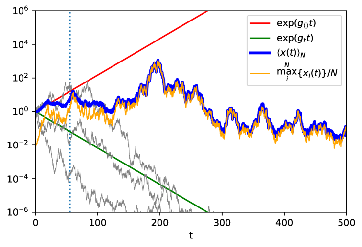
Figure 1: PEA and maximum in a finite ensemble of size $N=256$. Red line: expectation value $\left\langle x(t)\right\rangle$. Green line: exponential growth at the time-average growth rate. In the $T\to\infty$ limit all trajectories grow at this rate. Yellow line: contribution of the maximum value of any trajectory at time $t$ to the PEA. Blue line: PEA $\left\langle x(t)\right\rangle_{N}$. Vertical line: Crossover – for $t>t_{c}=\frac{2\ln N}{\sigma^{2}}$ the maximum begins to dominate the PEA (the yellow line approaches the blue line). Grey lines: randomly chosen trajectories – any typical trajectory soon grows at the time-average growth rate. Parameters: $N=256$, $\mu=0.05$, $\sigma=\sqrt{0.2}$.

1.3 Our previous work on PEAs

In [10] we analysed PEAs of GBM analytically and numerically. Using Eq. (2) the PEA can be written as

$$\left\langle x\right\rangle_{N}=\frac{1}{N}\sum_{i=1}^{N}\exp\left[\left(\mu-\frac{\sigma^{2}}{2}\right)t+\sigma W^{(i)}(t)\right],$$ (14)

where $\left\{W^{(i)}(t)\right\}_{i=1\dots N}$ are $N$ independent realisations of the Wiener process. Taking the deterministic part out of the sum we re-write Eq. (14) as

$$\left\langle x\right\rangle_{N}=\exp\left[\left(\mu-\frac{\sigma^{2}}{2}\right)t\right]\frac{1}{N}\sum_{i=1}^{N}\exp\left(t^{1/2}\sigma\xi_{i}\right),$$ (15)

where $\left\{\xi_{i}\right\}_{i=1\dots N}$ are $N$ independent standard normal variates.

We found that typical trajectories of PEAs grow at $g_{\left\langle\right\rangle}$ up to a time $t_{c}$ that is logarithmic in $N$, meaning $t_{c}\propto\ln N$. This is consistent with our sketch in Sec. (1.2). After this time, typical PEA-trajectories begin to deviate from expectation-value behavior, and eventually their growth rate converges to $g_{t}$. While the two limiting behaviours $N\to\infty$ and $t\to\infty$ can be computed exactly, what happens in between is less straight-forward. The PEA is a random object outside these limits. In [10] we dealt with this issue numerically by creating a super-sample of $S$ samples, each consisting of $N$ trajectories. In this way we were able to study the median of $\left\langle x\right\rangle_{N}(t)$, representing the behavior of typical trajectories.

A quantity of crucial interest to us is the exponential growth rate experienced by the PEA,

$$g_{\text{est}}(t,N)\equiv\frac{\ln(\left\langle x(t)\right\rangle_{N})-\ln(x(0))}{t-0}=\frac{1}{t}\ln(\left\langle x(t)\right\rangle_{N}).$$ (16)

In [10] we proved that the $t\to\infty$ limit for any (finite) $N$ is the same as for the case $N=1$,

$$\lim_{t\to\infty}g_{\text{est}}(t,N)=\mu-\frac{\sigma^{2}}{2}$$ (17)

for all $N\geq 1$. Substituting Eq. (15) in Eq. (16) produces

$$g_{\text{est}}(t,N) = \mu-\frac{\sigma^{2}}{2}+\frac{1}{t}\ln\left(\frac{1}{N}\sum_{i=1}^{N}\exp(t^{1/2}\sigma\xi_{i})\right)$$ (18)

$$= \mu-\frac{\sigma^{2}}{2}-\frac{\ln N}{t}+\frac{1}{t}\ln\left(\sum_{i=1}^{N}\exp(t^{1/2}\sigma\xi_{i})\right).$$ (19)

We didn’t look in [10] at the expectation value of $g_{\text{est}}(t,N)$ for finite time and finite samples, but it’s an interesting object that depends on $N$ and $t$ but is not stochastic. Note that this is not $g_{\text{est}}$ of the expectation value, which would be the $N\to\infty$ limit of Eq. (16). Instead it is the $S\to\infty$ limit,

$$\left\langle g_{\text{est}}(t,N)\right\rangle=\frac{1}{t}\left\langle\ln(\left\langle x(t)\right\rangle_{N})\right\rangle=f(N,t),$$ (20)

where, as in Sec. (1.2), $\left\langle\cdot\right\rangle$ without subscript refers to the average over all possible samples, i.e. $\lim_{S\to\infty}\left\langle\cdot\right\rangle_{S}$. The last two terms in Eq. (19) suggest an exponential relationship between ensemble size and time. The final term is a tricky stochastic object on which the properties of the expectation value in Eq. (20) will hinge. This term will be the focus of our attention: the sum of exponentials of normal random variates or, equivalently, log-normal variates.

2 Mapping to the random energy model

Since the publication of [10] we have learned, thanks to discussions with J.-P. Bouchaud, that the key object in Eq. (19) – the sum of exponentials of normal random variates – has been of interest to the mathematical physics community since the 1980s.

The reason for this is Derrida’s random energy model [5, 6]. It is defined as follows. Imagine a system whose energy levels are $2^{K}=N$ random numbers $\xi_{i}$ (corresponding to $K=\ln N/\ln 2$ spins). This is a very simple model of a disordered system, such as a spin glass, the idea being that the system is so complicated that we “give up” and just model its energy levels as realizations of a random variable. (We denote the number of spins by $K$ and the number of resulting energy levels by $N$, whereas Derrida uses $N$ for the number of spins). The partition function is then

$$Z=\sum_{i=1}^{N}\exp\left(\beta J\sqrt{\frac{K}{2}}\xi_{i}\right),$$ (21)

where the inverse temperature, $\beta$, is measured in appropriate units, and the scaling in $K$ is chosen so as to ensure an extensive thermodynamic limit [5, p. 79]. $J$ is a constant that will be determined below. The logarithm of the partition function gives the Helmholtz free energy,

$$F = -\frac{\ln Z}{\beta}$$ (22)

$$= -\frac{1}{\beta}\ln\left[\sum_{i=1}^{N}\exp\left(\beta J\sqrt{\frac{K}{2}}\xi_{i}\right)\right].$$ (23)

Like the growth rate estimator in Eq. (16), this involves a sum of log-normal variates and, indeed, we can rewrite Eq. (19) as

$$g_{\text{est}}=\mu-\frac{\sigma^{2}}{2}-\frac{\ln N}{t}-\frac{\beta F}{t},$$ (24)

which is valid provided that

$$\beta J\sqrt{\frac{K}{2}}=\sigma t^{1/2}.$$ (25)

Equation (25) does not give a unique mapping between the parameters of our GBM, $(\sigma,t)$, and the parameters of the REM, $(\beta,K,J)$. Equating (up to multiplication) the constant parameters, $\sigma$ and $J$, in each model gives us a specific mapping:

$$\sigma=\frac{J}{\sqrt{2}}\quad\text{and}\quad t^{1/2}=\beta\sqrt{K}.$$ (26)

The expectation value of $g_{\text{est}}$ is interesting. The only random object in Eq. (24) is $F$. Knowing $\left\langle F\right\rangle$ thus amounts to knowing $\left\langle g_{\text{est}}\right\rangle$. In the statistical mechanics of the random energy model $\left\langle F\right\rangle$ is of key interest and so much about it is known. We can use this knowledge thanks to the mapping between the two problems.

Derrida identifies a critical temperature,

$$\frac{1}{\beta_{c}}\equiv\frac{J}{2\sqrt{\ln 2}},$$ (27)

above and below which the expected free energy scales differently with $K$ and $\beta$. This maps to a critical time scale in GBM,

$$t_{c}=\frac{2\ln N}{\sigma^{2}},$$ (28)

with high temperature ($1/\beta>1/\beta_{c}$) corresponding to short time ($t<t_{c}$) and low temperature ($1/\beta<1/\beta_{c}$) corresponding to long time ($t>t_{c}$). Note that $t_{c}$ in Eq. (28) scales identically with $N$ and $\sigma$ as the transition time, Eq. (12), in our sketch.

In [5], $\left\langle F\right\rangle$ is computed in the high-temperature (short-time) regime as

$$\left\langle F\right\rangle = E-S/\beta$$ (29)

$$= -\frac{K}{\beta}\ln 2-\frac{\beta KJ^{2}}{4},$$ (30)

and in the low-temperatures (long-time) regime as

$$\left\langle F\right\rangle=-KJ\sqrt{\ln 2}.$$ (31)

Short time
We look at the short-time behavior first (high $1/\beta$, Eq. (30)). The relevant computation of the entropy $S$ in [5] involves replacing the number of energy levels $n(E)$ by its expectation value $\left\langle n(E)\right\rangle$. This is justified because the standard deviation of this number is $\sqrt{n}$ and relatively small when $\left\langle n(E)\right\rangle>1$, which is the interesting regime in Derrida’s case.

For spin glasses, the expectation value of $F$ is interesting, supposedly, because the system may be self-averaging and can be thought of as an ensemble of many smaller sub-systems that are essentially independent. The macroscopic behavior is then given by the expectation value.

Taking expectation values and substituting from Eq. (30) in Eq. (24) we find

$$\left\langle g_{\text{est}}\right\rangle^{\text{short}}=\mu-\frac{\sigma^{2}}{2}+\frac{1}{t}\frac{KJ^{2}}{4T^{2}}.$$ (32)

From Eq. (25) we know that $t=\frac{KJ^{2}}{2\sigma^{2}T^{2}}$, which we substitute, to find

$$\left\langle g_{\text{est}}\right\rangle^{\text{short}}=\mu,$$ (33)

which is the correct behavior in the short-time regime.

Long time
Next, we turn to the expression for the long-time regime (low temperature, Eq. (31)). Again taking expectation values and substituting, this time from Eq. (31) in Eq. (24), we find for long times

$$\left\langle g_{\text{est}}\right\rangle^{\text{long}}=\mu-\frac{\sigma^{2}}{2}-\frac{\ln{N}}{t}+\sqrt{\frac{2\ln N}{t}}\,\sigma,$$ (34)

which has the correct long-time asymptotic behavior. The form of the correction to the time-average growth rate in Eq. (34) is consistent with [10] and [11], where it was found that approximately $N=\exp(t)$ systems are required for ensemble-average behavior to be observed for a time $t$, so that the parameter $\ln N/t$ controls which regime dominates – if the parameter is small, then Eq. (34) indicates that the long-time regime is relevant.

Figure  2 is a direct comparison between the results derived here, based on [5], and numerical results using the same parameter values as in [10], namely $\mu=0.05,\sigma=\sqrt{0.2},N=256$ and $S=10^{5}$.

Notice that $\left\langle g_{\text{est}}\right\rangle$ is not the (local) time derivative $\frac{\partial}{\partial t}\left\langle\ln(\left\langle x\right\rangle_{N})\right\rangle$, but a time-average growth rate, $\left\langle\frac{1}{t}\ln\left(\frac{\left\langle x(t)\right\rangle_{N}}{\left\langle x(0)\right\rangle_{N}}\right)\right\rangle$. In [10] we used a notation that we’ve stopped using since then because it caused confusion – $\left\langle g\right\rangle$ there denotes the growth rate of the expectation value, which is not the expectation value of the growth rate.

It is remarkable that the expectation value $\left\langle g_{\text{est}}(N,t)\right\rangle$ so closely reflects the median, $q_{0.5}$, of $\left\langle x\right\rangle_{N}$, in the sense that

$$q_{0.5}(\left\langle x(t)\right\rangle_{N})\approx\exp\left(\left\langle g_{\text{est}}(N,t)\right\rangle t\right).$$ (35)

In [9] it was discussed in detail that $g_{\text{est}}(1,t)$ is an ergodic observable for Eq. (1), in the sense that $\left\langle g_{\text{est}}(1,t)\right\rangle=\lim_{t\to\infty}g_{\text{est}}$. The relationship in Eq. (35) is far more subtle. The typical behavior of GBM PEAs is complicated outside the limits $N\to\infty$ or $t\to\infty$, in the sense that growth rates are time dependent here. This complicated behavior is well represented by an approximation that uses physical insights into spin glasses. Beautiful!

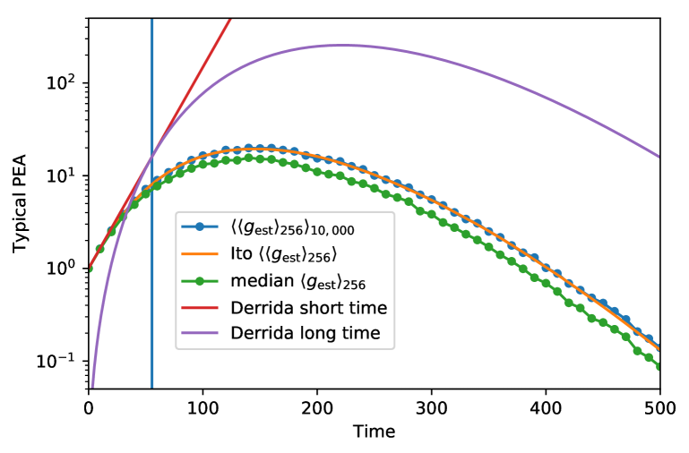
Figure 2: Lines are obtained by exponentiating the various exponential growth rates. Blue line: $\left\langle\left\langle g_{\text{est}}\right\rangle_{256}\right\rangle_{10,000}$ is the numerical mean (approximation of the expectation value) over a super-ensemble of $S=10,000$ samples of $g_{\text{est}}$ estimated in sub-ensembles of $N=256$ GBMs each. Green line: median in a super-ensemble of $S$ samples of $g_{\text{est}}$, each estimated in sub-ensembles of size $N$. Yellow line: Eq. (45) is an exact expression for $d\left\langle\ln\left\langle x\right\rangle_{N}\right\rangle$, derived using Itô calculus. We evaluate the expression by Monte Carlo, and integrate, $\left\langle\ln\left\langle x\right\rangle_{N}\right\rangle=\int_{0}^{t}d\left\langle\ln\left\langle x\right\rangle_{N}\right\rangle$. Exponentiation yields the yellow line. Red line: short-time behavior, based on the random energy model, Eq. (33). Purple line: long-time behavior, based on the random energy model, Eq. (34). Vertical line: Crossover between the regimes at $t_{c}=\frac{2\ln N}{\sigma^{2}}$, corresponding to $\beta_{c}=\frac{2(\ln 2)^{1/2}}{J}$. Parameters: $N=256$, $S=10,000$, $\mu=0.05$, $\sigma=\sqrt{0.2}$.

3 Another route via Itô calculus

Another way to find the expectation value of PEA growth rates, Eq. (20), is to compute $\left\langle d\ln\left\langle x\right\rangle_{N}\right\rangle$ using Itô calculus. We compute this directly, without invoking the random energy model. To apply Itô calculus, we will need the first two partial derivatives of $d\ln\left\langle x\right\rangle_{N}$ with respect to $x_{i}$.

$$\frac{\partial\ln\left\langle x\right\rangle_{N}}{\partial x_{i}}=\frac{1}{N\left\langle x\right\rangle_{N}}$$ (36)

and

$$\frac{\partial^{2}\ln\left\langle x\right\rangle_{N}}{\partial x_{i}^{2}}=-\frac{1}{N^{2}\left\langle x\right\rangle_{N}^{2}}$$ (37)

Now, Taylor-expanding $d\ln\left\langle x\right\rangle_{N}$ we find

$$d\ln\left\langle x\right\rangle_{N} = \sum_{i}\frac{\partial\ln\left\langle x\right\rangle_{N}}{\partial x_{i}}dx_{i}+\frac{1}{2}\sum_{i}\sum_{j}\frac{\partial^{2}\ln\left\langle x\right\rangle_{N}}{\partial x_{i}\partial x_{j}}dx_{i}dx_{j}+\ldots$$ (38)

$$\approx \frac{1}{N\left\langle x\right\rangle_{N}}\sum_{i}dx_{i}-\frac{1}{2N^{2}\left\langle x\right\rangle_{N}^{2}}\sum_{i}\sum_{j}dx_{i}dx_{j}.$$ (39)

The double-sum can be split into ‘diagonal’ ($i=j$) terms and cross-terms as

$$\frac{1}{N\left\langle x\right\rangle_{N}}\sum_{i}x_{i}(\mu dt+\sigma dW_{i})-\frac{1}{2N^{2}\left\langle x\right\rangle_{N}^{2}}\left(\sum_{i}dx_{i}^{2}+\sum_{j}\sum_{i\neq j}dx_{i}dx_{j}\right)\hskip 17.07182pt$$ (40)

Parts of the cross-terms are negligible because they are of order $dt^{2}$ and the rest vanishes when taking the expectation value, as we see by writing out one cross term

$$dx_{i}dx_{j}=x_{i}x_{j}(\mu^{2}dt^{2}+\mu\sigma dtdW_{i}+\mu\sigma dtdW_{j}+\sigma^{2}dW_{i}dW_{j}).$$ (41)

We therefore drop these terms now, as we take the expectation value, using the Wiener identity $\left\langle dW_{i}^{2}\right\rangle=dt$ for the final term

$$\left\langle d\ln\left\langle x\right\rangle_{N}\right\rangle = \left\langle\mu dt-\frac{1}{2N^{2}\left\langle x\right\rangle_{N}^{2}}\sum_{i}x_{i}^{2}(\mu^{2}dt^{2}+\sigma^{2}dt)\right\rangle$$ (42)

$$= \mu dt-\left\langle\frac{1}{2}\sigma^{2}\frac{\left\langle x^{2}\right\rangle_{N}}{N\left\langle x\right\rangle_{N}^{2}}\right\rangle dt+O(dt^{2}).$$ (43)

Discarding terms of higher-than-first order in $dt$ and re-writing the last term as a fraction of sums, we thus have

$$\frac{\left\langle d\ln\left\langle x\right\rangle_{N}\right\rangle}{dt} = \mu-\frac{1}{2}\sigma^{2}\left\langle\frac{\frac{1}{N}\sum_{i}x_{i}^{2}}{N\left(\frac{1}{N}\sum_{i}x_{i}\right)^{2}}\right\rangle$$ (44)

$$= \mu-\frac{1}{2}\sigma^{2}\left\langle\frac{\sum_{i}x_{i}^{2}}{\left(\sum_{i}x_{i}\right)^{2}}\right\rangle$$ (45)

This expression has the correct behaviour: for short times, all $x_{i}$ are essentially identical, and the second term is $-\frac{1}{2}\sigma^{2}\frac{1}{N}$, which is negligible if $N$ is large. So, for short times we see expectation-value behaviour. For long times, the largest $x_{i}$ will dominate both the numerator and the denominator, and we have $-\frac{1}{2}\sigma^{2}$: the full Itô correction is felt for long times.

4 Discussion

The Itô result is exact. A Monte-Carlo estimate of Eq. (45) (which is easy to obtain) is shown in Fig. 2 (yellow line). This agrees well with numerical observations. The approximations from the random energy model have the right shape and asymptotic behavior, though they’re not on the same scale as the median PEA. This is, of course, not surprising because these estimates are not designed to coincide with the median PEA. Quantitatively they are closer to a higher quantile of the distribution of PEAs. An intriguing question is this: is our computation using Itô calculus helpful to compute the expected free energy of the random energy model?

References

- [1] A. Adamou and O. Peters. Dynamics of inequality. Significance, 13(3):32–35, 2016.
- [2] Y. Berman, O. Peters, and A. Adamou. An empirical test of the ergodic hypothesis: Wealth distributions in the United States. January 2017. Available at SSRN: https://ssrn.com/abstract=2794830.
- [3] J.-P. Bouchaud. On growth-optimal tax rates and the issue of wealth inequalities. http://arXiv.org/abs/1508.00275, August 2015.
- [4] J.-P. Bouchaud and M. Mézard. Wealth condensation in a simple model of economy. Physica A, 282(4):536–545, 2000.
- [5] B. Derrida. Random-energy model: Limit of a family of disordered models. Phys. Rev. Lett., 45(2):79–82, July 1980.
- [6] B. Derrida. Random-energy model: An exactly solvable model of disordered systems. Phys. Rev. B, 24:2613–2626, September 1981.
- [7] H. Morowitz. Beginnings of cellular life. Yale University Press, 1992.
- [8] O. Peters and A. Adamou. The evolutionary advantage of cooperation. arXiv:1506.03414, June 2015.
- [9] O. Peters and M. Gell-Mann. Evaluating gambles using dynamics. Chaos, 26:23103, February 2016.
- [10] O. Peters and W. Klein. Ergodicity breaking in geometric Brownian motion. Phys. Rev. Lett., 110(10):100603, March 2013.
- [11] S. Redner. Random multiplicative processes: An elementary tutorial. Am. J. Phys., 58(3):267–273, March 1990.