Tuning Streamed Applications on Intel Xeon Phi:
A Machine Learning Based Approach

Abstract

Many-core accelerators, as represented by the XeonPhi coprocessors and GPGPUs, allow software to exploit spatial and temporal sharing of computing resources to improve the overall system performance. To unlock this performance potential requires software to effectively partition the hardware resource to maximize the overlap between host-device communication and accelerator computation, and to match the granularity of task parallelism to the resource partition. However, determining the right resource partition and task parallelism on a per program, per dataset basis is challenging. This is because the number of possible solutions is huge, and the benefit of choosing the right solution may be large, but mistakes can seriously hurt the performance. In this paper, we present an automatic approach to determine the hardware resource partition and the task granularity for any given application, targeting the Intel XeonPhi architecture. Instead of hand-crafting the heuristic for which the process will have to repeat for each hardware generation, we employ machine learning techniques to automatically learn it. We achieve this by first learning a predictive model offline using training programs; we then use the learned model to predict the resource partition and task granularity for any unseen programs at runtime. We apply our approach to 23 representative parallel applications and evaluate it on a CPU-XeonPhi mixed heterogenous many-core platform. Our approach achieves, on average, a 1.6x (upto 5.6x) speedup, which translates to 94.5% of the performance delivered by a theoretically perfect predictor.

I Introduction

Heterogeneous many-core systems are now commonplace [1]. The combination of using a host CPU together with specialized processing units (e.g., GPGPUs or the Intel XeonPhi) has been shown in many cases to achieve orders of magnitude performance improvement. Typically, the host CPU of a heterogeneous platform manages the execution context while the computation is offloaded to the accelerator or coprocessor. Effectively leveraging such platforms not only enables the achievement of high performance, but also increases the energy efficiency.

While the heterogeneous many-core design offers the potential for energy-efficient, high-performance computing, software developers are finding it increasingly hard to deal with the complexity of these systems [2]. In particular, programmers need to effectively manage the host-device communication, because the communication overhead can completely eclipse the benefit of computation off-loading if not careful [3, 4, 5]. Heterogeneous streaming has been proposed as a solution to amortize the host-device communication cost [6]. It works by partitioning the processor cores to allow independent communication and computation tasks (i.e. streams) to run concurrently on different hardware resources, which effectively overlaps the kernel execution with data movements. Representative heterogeneous streaming implementations include CUDA Streams [7], OpenCL Command Queues [8], and Intel’s hStreams [9, 6]. These implementations allow the program to spawn more than one stream/pipeline so that the data movement stage of one pipeline overlaps the kernel execution stage of another.

Prior work on heterogeneous streams mainly targets GPUs [10, 11, 12]. While also offering heterogeneous stream execution, the OS-enabled Intel XeonPhi coprocessor provides some unique features that are currently unavailable on the GPU. For example, beside specifying the number of streams , developers can explicitly map streams to different groups of cores on XeonPhi to control the number of cores of each hardware partition. This parameter is not exposed to programmers on GPUs, making previous work on GPU-based stream optimizations infeasible to fully exploit XeonPhi (see also Section V-C). One the other hand, there are ample evidences showing that choosing the right stream configuration, i.e., the number of processor core partitions and the number of concurrent tasks of a streamed application, values, has a significant impact on the streamed application’s performance on XeonPhi [13, 14]. However, attempting to find the optimum values through exhaustive search would be ineffective, because the range of the possible values for the two parameters is huge. What we need is a technique that automatically determines the optimal stream configuration for any streamed application in a fast manner.

This paper presents a novel runtime approach to determine the right number of partitions and tasks for heterogeneous streams, targeting the Intel XeonPhi architecture. We do so by employing machine learning techniques to automatically construct a predictive model to decide at runtime the optimal stream configuration for any streamed application. Our predictor is first trained off-line. Then, using code and dynamic runtime features of the program, the model predicts the best configuration for a new, unseen program. Our approach avoids the pitfalls of using a hard-wired heuristic that requires human modification every time when the architecture evolves, where the number and the type of cores are likely to change from one generation to the next.

We apply our approach to 23 representative benchmarks, and evaluate it on a heterogeneous many-core platform that has a general purposed multi-core CPU and a 57-core Intel XeonPhi coprocessor. Our approach achieves, on average, a 1.6x speedup over the optimized, non-streamed code. This translates to 94.5% of the best available performance.

We make the following technical contributions:

• We present the first machine learning model for automatically determining the optimal stream configuration on Intel XeonPhi. Note that we do not seek to advance the machine learning algorithm itself; instead, we show how machine learning can be used to address the challenging problem of tuning stream configurations;

• We develop a fully automatic approach for feature selection and training data generation;

• We show that our approach delivers constantly better performance over the single-streamed execution across programs and inputs;

• Our approach is immediately deployable and does not require any modification to the application source code.

II Background and Overview

In this section, we first give a brief introduction of heterogeneous streams; we then define the scope of this work, before motivating the need of our scheme and providing an overview of our approach.

II-A Heterogeneous Streams

The idea of heterogeneous streams is to exploit temporal and spatial sharing of the computing resources.

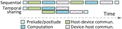
Figure 1: Exploit pipeline parallelism through temporal sharing.

Temporal Sharing. Code written for heterogeneous computing devices typically consists of several stages such as host device communication and computation. Using temporal sharing, one can overlap some of these stages to exploit pipeline parallelism to improve performance. This paradigm is illustrated in Figure 1. In this example, we can exploit temporal sharing to overlap the host-device communication and computation stages to achieve better runtime when compared to execute every stage sequentially. One way of exploiting temporal sharing is to divide an application into independent tasks so that they can run in a pipeline fashion.

Spatial Sharing. Modern many-core accelerators offer a large number of processing units. Since many applications cannot fully utilize all the cores at a time, we can partition the computing units into multiple groups to concurrently execute multiple tasks. In this way, the computing resource is spatially shared across concurrently-running application tasks. The key to spatial sharing is to determine the right number of partitions, because over-provisioning of processing units would waste computing resources but under-provisioning would lead to slowed down performance.

⬇ 1//setting the partition-size and task granularity hStreams_app_init(partition_size,streams_p_part); 3 //stream queue id 5stream_id = 0; for(…){ 7 //enquque host-device transfer to current stream hStreams_app_xfer_memory(,,, stream_id, HSTR_SRC_TO_SINK,…); 9 … //enqueue computation to the current stream 11 hStreams_EnqueueCompute(stream_id, ”kernel1”, …); … 13 //move to the next stream stream_id = (stream_id++) % MAX_STR; 15} //transfer data back to host 17hStreams_app_xfer_memory(,,, HSTR_SINK_TO_SRC,…);

Figure 2: Example hStreams code.

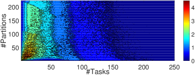
(a) binomial

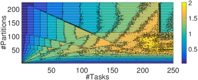
(b) prefixsum

Figure 3: Heatmaps show the resultant speedup (over non-streamed) of binomial and prefixsum under different stream configurations. The #partitions and #tasks have a significant impact on the resultant performance, and the sweat spots are sparse and vary across programs.

II-B Problem Scope

Our work aims to improve the performance of a data parallel application by exploiting spatial and temporal sharing of heterogeneous streams. We do so by determining at runtime how many partitions should be used to group the cores (#partitions) and how many data parallel tasks (#tasks) should be used to run the application. We target the Intel XeonPhi architecture, but our methodology is generally applicable and can be extended to other architectures including GPGPUs and FPGAs.

Code Example. Figure 2 gives a simplified code example written with Intel’s hStreams APIs. At line 2 we initialize the stream execution by setting the number of partitions and tasks/streams per partition. This initialization process essentially creates multiple processor domains and determines how many logical streams can run on a partition. In the for loop (lines 7-14) we enqueue the communication and computation tasks to a number of streams identified by the stream_id variable. In this way, communication and computation of different streams can be overlapped during execution (temporal sharing); and streams on different processor domains (or partitions) can run concurrently (spatial sharing). Our predictive model determines the #partitions and the #tasks before invoking the hStreams initialization routine, hStreams_app_init(). We also create a wrap for this API to automatically invoke our predictive model, so no modification to the application source code is required.

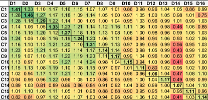
Figure 4: Colour table showing the speedups of best-performing configurations across inputs for dct. Each cell shows the performance for one of the 16 best-performing configurations, $Cn$, on a given input, $Dn$. The best configuration varies across inputs and a good configuration on one input can give poor performance on another dataset.

II-C Motivating Examples

Consider Figure 3 which shows the resultant performance improvement over the non-streamed version of the code for two applications on a 57-core Intel XeonPhi system. It is observed from this example that no all stream configurations give improved performance. As can be seen from the diagrams, the search space of stream configuration is huge but good configurations are sparse. The performance varies significantly over stream configurations (#partitions, #tasks). The optimal #tasks for binomial ranges from 1 to 30, and the best #partitions is between 1 and 40. In contrast to binomial, prefixsum benefits from fine-grained parallelism when using a larger #tasks (220 to 224) and #partitions (60 to 80). However, the stream configurations that are effective for prefixsum give no speedup over the non-streamed version for binomial.

Now consider Figure 4 that shows the speedups of dct under 16 configurations over the non-streamed version, where each configuration is found to give the best-performance for one of the 16 inputs. In the color table, each cell shows the performance of a stream configuration ($C1,...,C16$) on a specific input dataset ($D1,...,D16$); and the values along the diagonal line represent the best-available performance for an input. As can be seen from the figure, the best stream configuration can vary across inputs for the same benchmark. For example, while $C4$ gives 1.33 speedup for dataset $D4$, it delivers a poor performance for dataset $D14$ by doubling the execution time over the non-streamed version. This diagram also suggests that none of the 16 configurations gives improved performance for all inputs.

Lesson Learned. These two examples demonstrate that choosing the stream configuration has a great impact on the resultant performance and the best configuration must be determined on a per-program and per-dataset basis. Attempting to find the optimal configuration through means of an exhaustive search would be ineffective, the overhead involved would be far bigger than the potential benefits. Online search algorithms, while can speedup the search process, the overhead can still outweigh the benefit. For example, when applying simulated annealing to binomial, the best-found configuration only reaches 84% of the best-available performance after 310,728 iterations. Classical hand-written heuristics are not ideal either, as they are not only complex to develop, but are likely to fail due to the variety of programs and the ever-changing hardware architecture. An alternate approach, and the one we chose to use, is to use machine learning to automatically construct a predictive model directly predict the best configuration, providing minimal runtime, and having little development overhead when targeting new architectures.

II-D Overview

Our library-based approach, depicted in Figure 5, is completely automated. To determine the best streaming configuration, our approach follows a number of steps described as follows. We use a set of information or features to capture the characteristics of the program. We develop a LLVM [15] compiler pass to extract static code features at compile time, and a low-overhead profiling pass to collect runtime information at execution time. Because profiling also contributes to the final program output, no computation cycle is wasted. At runtime, a predictive model (that is trained offline) takes in the feature values and predicts the optimal stream configuration. The overhead of runtime feature collection and prediction is a few milliseconds, which is included in all our experimental results.

Figure 5: Our machine learning based model predicts the optimal stream configuration based on the code and runtime features.

III Predictive Modeling

Our model for predicting the best stream configuration is a Support Vector Machine (SVM) with a quadratic function kernel. The model is implemented using libSVM (C++ version) [16]. We have evaluated a number of alternative modeling techniques, including regression, K-Nearest neighbour (KNN), decision trees, and the artificial neural network (ANN), etc. We chose SVM because it gives the best performance and can model both linear and non-linear problems (Section V-D2). The model takes in feature values and produces a label for the optimal stream configuration.

Building and using such a model follows a 3-step process for supervised learning: (i) generate training data (ii) train a predictive model (iii) use the predictor, described as follows.

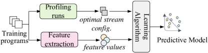
Figure 6: The training process of our approach

III-A Training the Predictor

Our method for model training is shown in Figure 6. To learn a new predictor we first need to find the best stream configuration for each training program, and extract the feature values from the program. We then use this set of feature values and optimal configurations to train a model.

III-A1 Generating Training Data

We use cross validation by excluding the testing benchmarks from the training dataset. To generate the training data for our model we used 15 programs. We execute each training program and benchmark a number of times until the gap of the upper and lower confidence bounds is smaller than 5% under a 95% confidence interval setting. We exhaustively execute each training program across all of our considered stream configurations, and record the performance of each. Specifically, we profile the program using the #partitions ranging from 1 to 224 and the #tasks ranging from 1 to 256 . Next, we record the best performing configuration for each program and dataset, keeping a label of each. Finally, we extract the values of our selected set of features from each program and dataset.

Data Labeling. Our initial labeling process generates over 100 labels while we only have a small number of training samples. The expected predicting accuracy is deemed to be low as some of the labels only have a handful of examples. Therefore, we have to merge labels after generating the raw training data. Our label merging procedure is shown in Algorithm 1. This merging process aims to reduce the number of labels to an order of magnitude less than that of samples (from $N$ to a configurable parameter $Nr$). The input are the training samples, each with a set of well-performing stream configurations (e.g., the top 3% best-performing configurations). We calculate the similarity of two labels using three quantitative metrics: (a) the common best configurations (we aim to keep the common best configurations), (b) whether the samples are from the same program, and (c) whether they are with the same dataset. The three metrics are denoted by $\omega_{1}$, $\omega_{2}$, and $\omega_{3}$ respectively in Algorithm 1. We discuss the performance impact of the label merging algorithm in Section V-D1. Then, we sort the weights in a descending order, merge corresponding labels, and update the label for each sample. The output samples are labeled with merged classes. Applying the data labeling process described above results in 28 labels (i.e., $Nr$=28).

Algorithm 1 The Label Merging Algorithm.

1:input: LS – label set, PS – program set, DS – dataset

2:output: LSr – reduced label set

3:procedure Merging_Labels($LS$, $PS$, $DS$, $N$; $LSr$, $Nr$)

4:       $LSr\leftarrow LS,Nr\leftarrow N$

5:       repeat

6:             for $s\leftarrow 0,Nr$ do

7:                   for $t\leftarrow 0,Nr$ do

8:                         $p_{s}\leftarrow PID(PS,s),p_{t}\leftarrow PID(PS,t)$

9:                         $d_{s}\leftarrow DID(DS,s),d_{t}\leftarrow DID(DS,t)$

10:                         if $s\neq t$ then

11:                               $w_{1},w_{2},w_{3}\leftarrow 0$

12:                               $LS_{st}\leftarrow LS_{s}\sqcap LS_{t}$

13:                               $w_{1}\leftarrow Counts(LS_{st})$

14:                               if $p_{s}==p_{t}$ then $\triangleright$ the same program

15:                                     $w_{2}\leftarrow 150$

16:                               end if

17:                               if $d_{s}==d_{t}$ then $\triangleright$ the same dataset

18:                                     $w_{3}\leftarrow 30$

19:                               end if

20:                               $w(s,t)\leftarrow w_{1}+w_{2}+w_{3}$

21:                         end if

22:                   end for

23:             end for

24:             $RankOnWeight(w)$ $\triangleright$ Rank w on the weights

25:             $MergeAndUpdate(w,LS,N,LSr,Nr)$

26:       until $LS_{i}\sqcap LS_{j}=\phi,\forall i,j\in Nr\wedge i\neq j$

27:end procedure

III-A2 Building The Model

The corresponding configuration labels, along with the feature values for all training programs, are passed to a learning algorithm. The algorithm finds a correlation between the feature values and the optimal stream configuration. The output of our learning algorithm is a SVM model where the weights of the model are determined from the training data. We use the parameter tuning tool provided by libSVM to determine the kernel parameters. Parameter search is performed on the training dataset using cross-validation. In our case, the overall training process (which is dominated by training data generation) takes less than a week on a single machine. Since training is performed only once “at the factory”, this is a one-off cost.

III-B Features

Our predictive models are based exclusively on code and dynamic features of the target programs. Code features are extracted from the program source code, and dynamic features are collected using hardware performance counters during the initial profiling run of the target application. We restrict us to use hardware performance counters that are commonly available on modern processors such as the data cache misses to ensure that our approach can be applied to a wide range of architectures.

We considered 38 candidate raw features in this work. Some features were chosen from our intuition based on factors that can affect the performance such as dts (host-device data transfer size) and #xfer_mem, while other features were chosen based on previous work [17, 18].

III-B1 Feature Selection

To build an accurate predictive model through supervised learning, the training sample size typically needs to be at least one order of magnitude greater than the number of features. In this work, we start from 280 training samples and 38 raw features, so we would like to reduce the number of features in use. Our process for feature selection is fully automatic, described as follows. We first combine several raw features to form a set of combined normalized features, which are able to carry more information than the individual parts. For example, instead of reporting raw branch hit and miss counts we use the branch miss rate. Next, we removed raw features that carried similar information which is already captured by chosen features. To find which features are closely correlated we constructed a correlation coefficient matrix using the Pearson correlation coefficient. The closer a coefficient between two features is to +/-1, the stronger the correlation between the two input features. We removed any feature which had a correlation coefficient (taking the absolute value) greater than 0.7. Similar features include the number of executed instructions and the number of E-stage cycles that were successfully completed. Our feature selection process reduces the number of features to 10, which are listed in Table I. Since our approach for feature selection is automatic, the approach can be applied to other sets of candidate features. It is to note that feature selection is also performed using cross-validation (see also Section IV-B).

Table I: Final selected features.

Feature	Description
loop nest	at which level the loop can be parallelized
loop count	# of the parallel loop iterations
#xfer_mem	# of host-device transfer API calls
dts	total host-device transfer size
redundant transfer size	host-device transfer size among overlapping tasks
max blocks	the maximum number of tasks of the appliation
min task unit	the minimum task granularity for a partition
# instructions	the total number of instructions of the kernel
branch miss	branch miss rate
L1 DCR	L1 Data cache miss rate

III-B2 Feature Scaling

Supervised learning typically works better if the feature values lie in a certain range. Therefore, we scaled the value for each of our features between the range of 0 and 1. We record the maximum and minimum value of each feature found at the training phase, and use these values to scale features extracted from a new application after deployment.

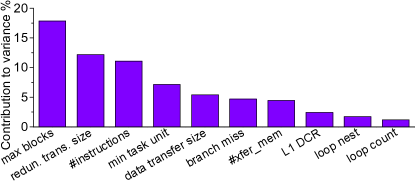
Figure 7: Feature importance according to the Varimax rotation.

III-B3 Feature Importance

To understand the usefulness of each selected feature, we apply a factor analysis technique called Varimax rotation [19] to the feature space transformed by the principal component analysis (PCA). This technique quantifies the contribution of each feature to the overall variance in each of the PCA dimensions. Intuitively, the more variances a feature brings to the space, the more useful information the feature carries. Features that capture the parallelism degree (e.g. max blocks), host-device communication (e.g. redundant transfer size), and computation (e.g. #instructions) are found to be important. Other features such as L1 DCR and loop nest are useful, but are less important compared to others. This figure shows that prediction can accurately draw upon a subset of aggregated feature values.

III-C Runtime Deployment

Once we have built and trained our predicted model as described above, we can use it to predict the best stream configuration for any new, unseen program. When an application is launched, we will first extract the feature values of the program. Code features (such as loop count) are extracted from the program source. Dynamic features (such as branch miss) are extracted by profiling the program without partitioning for several microseconds. After feature collection, we feed the feature values to the offline trained model which outputs a label indicating the stream configuration to use for the target program.

Adapt to Changing Program Phases. Our approach can adapt to different behaviors across kernels because predictions are performed on a per-kernel basis. It can be extended to adapt phase changes within a kernel. This can be achieved by checking periodically sampling if the performance counter readings are significantly different from the ones use for the initial prediction to trigger re-prediction and re-configuration. Dynamic re-configuration will require extending hStreams to adjust thread mapping and having hardware support to stop and resume the execution contexts.

IV Experimental Setup

IV-A Hardware, System Software and Benchmarks

Platform. Our evaluation platform is an Intel Xeon server with an Intel dual-socket 8-core Xeon CPU @ 2.6 Ghz (16 cores in total) and an Intel Xeon 31SP Phi accelerator (57 cores). The host CPUs and the accelerator are connected through PCIe. The host environment runs Redhat Linux v7.0 (with kernel v.3.10). The coprocessor environment runs a customized uOS (v2.6.38.8). We use Intel’s MPSS (v3.6) to communicate between the host and the coprocessor and Intel’s  hStreams library (v3.6).

Benchmarks. As currently there exist very few programs written with Intel’s hStreams, we faithfully translated 21 applications to hStreams from the commonly used benchmark suites. Table II gives the full list of these benchmarks. Among them, convolutionFFT2d and convolutionSeparable have algorithm-dependent parameters, which are regarded as different benchmarks in the experiments. This setting gives us a total of 23 programs. We run the majority of the programs using over 25 different datasets, except for some applications where we used around 10 datasets because the algorithmic constraints of the applications prevent us from generating a large number of inputs.

Table II: Programs used in our experiments.

Suite	Name	Acronym	Name	Acronym
	convol.Separable	convsepr1(8)	dotProduct	dotprod
	convolutionFFT2d	fftx1y1(4y3)	fwt	fwt
	MonteCarlo	montecarlo	matVecMul	mvmult
	scalarProd	scalarprod	transpose	transpose
NVIDIA SDK	vectorAdd	vecadd
AMD SDK	binomial	binomial	BlackScholes	blackscholes
	dct	dct	prefixSum	prefix
	bfs	bfs	histo	histo
	lbm	lbm	mri-q	mri-q
	mri-gridding	mri-gridding	sad	sad
Parboil	sgemm	sgemm	spmv	spmv

IV-B Competitive Approaches

Because there is currently no expert-tuned heuristic for choosing stream configurations on XeonPhi, we compare our approach against two recent models for predicting the optimal stream configuration on GPUs. As it is currently not possible to configure the number of partitions on GPUs, the relevant models can only predict the number of tasks (or streams).

IV-B1 Liu et al.

In  [12], Liu et al. use linear regression models to search for the optimal number of tasks for GPU programs [12]. The approach employs several analytic models described as follows.

For a task with an input data size of $m$, the transferring time between the CPU and the GPU, $T_{t}$, is determined as $T_{t}=\alpha\cdot m+\beta$, and the computation time, $T_{c}$, is calculated as: $T_{c}=\eta\cdot m+\gamma$ where the model coefficients, $\alpha$, $\beta$, $\eta$ and $\gamma$, are determined through empirical experiments. For a given kernel with $N$ input data elements running using $n$ streams, this approach partitions the computation into $n$ tasks, where the data size for each task, $m$, is equal to $N$/$n$. Therefore, the total execution time, $T_{total}$, can be determined by:

$$T_{total}=T_{t}+nT_{c}=\alpha\cdot m+\frac{N\gamma}{m}+N\eta+\beta$$

By calculating the partial differential and second-order partial differential of $T_{total}$ with respect to $m$, we can obtain the optimal task-granularity as $m=\sqrt{\frac{N\gamma}{\alpha}}$. Then we can calculate the number of tasks ($n$). Note that, we set the #partitions to be the same as $n$ for XeonPhi.

IV-B2 Werkhoven et al.

The work presented by Werkhoven et al. models the performance of data transfers between the CPU and the GPU [10]. They use the LogGP model to estimate the host-device data transfer time. Specifically, the model estimates the data transfer time using five parameters: the communication latency ($L$), overhead ($o$), the gap ($g$), the number of processors ($P$), and the PCIe bandwidth ($G$).

Let $B_{hd}$ denotes the amount of data transferred from the host to the device and $B_{dh}$ denotes vice versa, and $T_{kernel}$ donates the kernel execution time. Then, the optimal number of streams (i.e., #tasks), $N_{s}$, can be estimated by solving the following equations:

$$B_{dh}*G_{dh}+g*(N_{s}-1)=\begin{cases}\frac{T_{kernel}}{N_{s}}+\frac{B_{dh}}{N_{s}}*G_{dh},&\text{if}B_{dh}>B_{hd}\\ \frac{B_{hd}}{N_{s}}*G_{hd}+\frac{T_{kernel}}{N_{s}},&\text{otherwise}\end{cases}$$

Again, for this model, we set the #partitions to be equal to the optimal $N_{s}$ value on XeonPhi.

IV-C Evaluation Methodology

Model Evaluation. We use cross-validation to evaluate our machine learning model. Our model is trained using benchmarks from the AMD and NVIDIA SDK suites, we then apply the trained model to benchmarks from the Parboil suite. We apply leave-one-out cross validation to the AMD and NVIDIA SDK suites. This means that we exclude the target program from the training program set, and learn a model using the remaining programs from the AMD and NVIDIA suites; we then then apply the learnt model to the testing program. We repeat this process to ensure each benchmark from the AMD and NVIDIA suites is tested. It is a standard evaluation methodology, providing an estimate of the generalization ability of a machine-learning model in predicting unseen data. Note that we exclude both convolutionFFT2d and convolutionSeparable from the training set when one of the two is evaluated.

Performance Report. We run each program under a stream configuration multiple times and report the geometric mean of the runtime. To determine how many runs are needed, we calculated the confidence range using a 95% confidence interval and make sure that the difference between the upper and lower confidence bounds is smaller than 5%.

V Experimental Results

In this section, we first present the overall performance of our approach. We then compare our approach to the fixed stream configuration and the two competitive approaches and before discussing the working mechanism of our scheme.

V-A Overall Performance

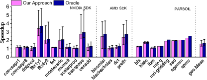
Figure 8: Overall performance compared to a single stream version. Our approach achieves, on average, 94.5% of the oracle performance. The min-max bars show the range of performance achieved across different inputs.

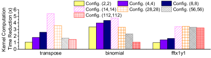
Figure 9: Reduction of kernel computation time over a single stream execution. The performance improvement comes from the reduction of the threading overhead. A stream configuration is annotated as (#partitions, #tasks).

In this experiment, we exhaustively profiled each application with all possible stream configurations and report the best-found performance as the Oracle performance. The Oracle performance gives an indication of how close our approach is to a theoretically perfect solution. The baseline used to calculate the speedup is running the application using a single stream without processor core partitioning.

V-A1 Overall Results

The result is shown in Figure 8. The min-max bar on the diagram shows the range of speedups per application across all evaluated inputs. Overall, our approach achieves an average speedup of 1.6$\times$ over the non-streamed code. This translates to 94.5% of the Oracle performance. Although our model is not trained on the Parboil benchmark suite, it achieves good performance, delivering 97.8% of the Oracle performance on this benchmark suite. This demonstrates the portability of our approach across benchmarks.

V-A2 Analysis of High Speedup Cases

We found that there are several benchmarks obtain a speedup of over 2$\times$. After having a closer investigation, we notice that such performance is because that streaming can also reduce the kernel execution time for these applications.

To quantify the benefit of kernel time reduction, we measure the kernel execution time with and without multiple streams and calculate the speedup between them. Note that we exclude the host-device communication time in this case. The kernel time improvement for transpose, binomial, and fftx1y1 is shown in Figure 9. As can be seen from the diagram, choosing a good stream configuration can lead to more than 4x reduction on the kernel execution time. This is because these benchmarks are implemented by parallelizing the inner loop within a nested loop. During runtime, the parallel threads working on the inner loop will need to be created, synchronized, or destroyed for each outer loop iteration. This threading overhead could be significant when the outer loop iterates many times. When using multiple streams, we essentially divide the whole outer loop iteration space into multiple smaller iteration space. This allows multiple groups of threads to be managed simultaneously, leading to a significant decrease in threading overhead and faster kernel execution time. On the other hand, we note that using too many streams and partitions will lead to a performance decrease. This is due to the fact that stream management also comes at a cost, which increases as the number of partitions increases. Nonetheless, for applications where the kernel computation domains the program execution time, by reducing the kernel time can lead to additional improvement, yielding more than 2x speedups.

V-A3 Speedup Distribution

We show the speedups per benchmark across datasets in Figure 10. The shape of the violin plot corresponds to the speedup distribution. We see that the speedups of montecarlo and prefix distribute fairly uniformly while the data distribution of fftx1y1 and fftx4y3 is multimodal (i.e. it has two peaks). Further, the input datasets have little impact on the behavior of fwt and lbm so the speedups remain constant across datasets. To conclude, the streaming speedups of some applications are sensitive to the input datasets while that of others are not.

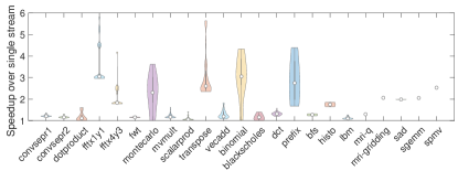
Figure 10: Violin plot showing the speedups per benchmark across datasets. The shape of the violin corresponds to the speedup distribution. The thick black line shows where 50% of the data lies.

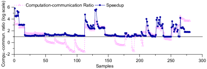
Figure 11: The relation between computation-communication ratio and the speedup. The computation-communication ratio is normalized using the natural logarithm function. Thus, the kernel computation time equals the host-device communication time when $ratio=0$. In general, a higher computation-communication ratio leads to a better speedup.

V-A4 Correlation Analysis

Figure 11 shows the relation between the computation-communication ratio and the achieved speedup when using heterogeneous streams across all benchmarks and datasets. We see that the computation-communication ratio varies over the benchmarks and the speedup changes accordingly, but in general a higher computation-to-communication ratio leads to a greater speedup. As explained in Section V-A2, in addition to overlapping the computation and communication, our approach can also reduce the kernel computation time by choosing the right stream configuration. Therefore, benchmarks with a high computation-communication ratio also benefit from a reduction in the kernel computation time.

To quantify the relation between the computation-communication ratio and the speedup, we calculate the Pearson correlation coefficient of the two variables. The calculation gives a correlation coefficient of 0.7, indicating that the two variables (the computation-communication ratio and the speedup) have a strong linear correlation. By carefully selecting the stream configuration, our approach tries to maximize the overlap between communication and computation, which thus leads to favourable performance.

Summary. The performance improvement of our approach comes from two factors. First, by predicting the right processor partition, our approach allows effective overlapping of the host-device communication and computation. Second, by matching task parallelism to the resource partition, our approach can reduce the overhead of thread management, compared to the single stream execution. When the host-device communication time dominates the streaming process, the performance improvement mainly comes from computation-communication overlapping and the speedup from streaming is consistantly less than 2$\times$. When the kernel execution time dominates the stream process, the application can benefit from the overhead reduction of thread management. In this case, the speedup can be as large as 5$\times$. This trend can be clearly seen from Figure 11.

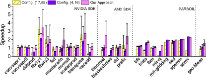
Figure 12: Comparing the performance with two fixed configurations: config. $(4,16)$ of 4 partitions and 16 tasks per partition, and config. $(17,85)$ of 17 partitions and 5 tasks per partition.

V-B Compare to Fixed Stream Configurations

A natural question to ask is that: is there a fixed stream configuration that gives reasonable good performance across benchmarks and datasets? To answer this question, we compare our predictive modeling based approach to two specific configurations. Our justification for using the two configurations are described as follows. Our initial results in Section II indicate that using the stream configuration of $(4,16)$, i.e. partitioning the cores to 4 groups and running 4 tasks on each partition (16 tasks in total), gives good performance. The statistics obtained from the training data suggest that the configuration of $(17,85)$ give the best averaged performance across training samples.

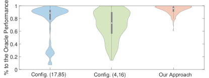
Figure 13: Violin plot showing the speedups per scheme across benchmarks and datasets. The shape of the violin corresponds to the speedup distribution to the oracle performance. The thick black line shows where 50% of the data lies.

Based on these two observations, we compare our adaptive approach to two configurations described above. The results are shown in Figure 12. We observe improved performance for several benchmarks such as mri-gridding, transpose, sad, under both configurations, but slowed down performance for dotprod, vecadd, blackscholes, lbm, and mir-q. For prefix, configuration $(17,85)$ delivers improved performance while configuration $(4,16)$ leads to slowed down performance. Overall, none of the two fixed configurations give an improved performance on average. On average, our approach outperforms the two fixed configurations by a factor of 1.4, and delivers consistently improved performance across benchmarks and datasets.

The violin plot in Figure 13 shows how far is each of the three schemes to the Oracle performance across benchmarks and datasets. Our approach not only delivers the closest performance to the Oracle, but also has the largest number of samples whose performance is next to the Oracle. By contrast, the performance given by the fixed configurations for many samples are further from the Oracle performance.

This experiment confirms that a fixed configuration fails to deliver improved performance across applications and datasets, and selecting a right stream configuration on a per program, per dataset basis is thus required.

V-C Compare to Alternated Models

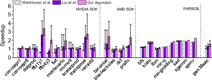
Figure 14: Comparing against Liu et al. and Werkhoven et al.

In this experiment, we compare our approach to the two recent analytical models described in Section IV-B. The results are shown in Figures 14 and 15. Both models prefer using $2$ tasks across benchmarks and datasets. This is because that the analytical models simply assume that task partition has no effect on kernel’s performance, and do not consider the thread management overhead.

From Figure 14, we see that our approach can obtain better performance for nearly all programs. For the remaining handful programs, all three approaches deliver comparable performance. Compare to Figure 12, we can find the performance of the analytical models is similar to fixed stream configurations. This is because the performance of the seven programs, such as binomial, changes dramatically with different stream configurations (see also Figure 3). The performance of the remaining programs is not sensitive to the variation of stream configurations. From Figure 15, we can further see that Liu et al. and Werkhoven et al. deliver a speedup within a range on 20% to 80%, while the performance of our approach is centralized on a range between 80% to 100%. Thus, our approach delivers consistently better performance compared with the alternative models.

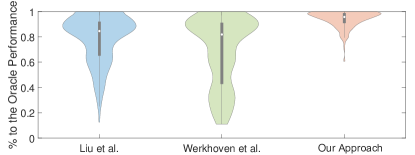
Figure 15: Violin plot showing the speedups per scheme across benchmarks and datasets. The shape of the violin corresponds to the speedup distribution to the oracle performance. The thick black line shows where 50% of the data lies.

V-D Model Analysis

V-D1 Evaluate the Label Merging Algorithm

To evaluate our label merging algorithm, we first use the 101 raw labels to train a predictive model. With the help of the label merging algorithm, we reduce the number of classes to be 28. Then we use the new labels to train a new predictor and compare the performance of these two models.

We show the result in Figure 16. We find that with the labels merge algorithm, the new predictive model performs, on average, 21% better than the one without label merging. It indicates that our label merging algorithm can lead to a better predictive performance by better balance training samples per stream configuration.

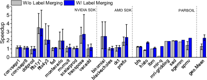
Figure 16: Resultant performance with and without label merging.

V-D2 Compare to Alternative Learning Techniques

Table III shows the average speedup achieved by different machine learning techniques. For each technique, we follow the same training methodology and use the same features and training examples to build a model. These schemes are implemented using scikit-learn [20] except for the SVM models which are built upon libSVM as our approach. We have performed parameter search on the training dataset to find the best performing model parameters. Specifically, we vary $k$ between 1 and 10 for KNN models and try different number of hidden layers and neurons for the ANN model.

Thanks to the high quality features, all models achieve similar performance (over 1.3x). Our SVM model based on a quadratic kernel function gives the best overall performance. This is because the kernel function we used can model both linear and non-linear relation between the features and the desired labels; and as a result, it predicts the best stream configuration more accurate than other alternative models. It is to note that the performance of the ANN model can be further improved if there are more training examples (e.g., through synthetic benchmark generation [21]) and our approach can be used with an ANN model without changing the learning process.

Table III: Compare to alternative learning techniques.

Learning techniques	Avg. speedup	Learning techniques	Avg. speedup
Gaussian SVM	1.37	Decision tree	1.39
Backpropagation ANN	1.42	Linear discriminant	1.40
Linear SVM	1.43	Ensemble KNN	1.44
Weighted KNN	1.45	Our approach	1.57

VI Related Work

Our work lies in the interaction of various areas: work partitioning, stream modeling, and predictive modeling.

Workload Partition. There is an extensive body of research work in distributing work across heterogeneous processors to utilize the computation resources to make program run faster [22, 23]. Prior work in the area typically assumes that the processor configuration is fixed and rely on the operating system to schedule parallel tasks across parallel processing units. Recent studies show that by partitioning the processing units into groups it is possible to significantly improve the application performance by overlapping the host-device communication and computation on coprocessors like Intel XeonPhi [14, 6]. However, existing approaches typically rely on manual tuning to find the processor partition and the best number of streams to run within a partition. As a result, previous approaches cannot adapt to the change of program behavior due to the change of program inputs. As a departure from prior work, this work develops an automatic approach to dynamically adjust the processor partition and task-granularity during runtime, considering the characteristics of applications and input datasets. As a result, our approach can adapt to the change of program behavior and runtime inputs.

Multiple Streams Modeling. Gomez-Luna et al. [11] develop a set of models to estimate the asynchronous data transfer overhead on different GPU architectures. The models can be used to estimate the optimal number of streams to use on a given GPU platform. Werkhoven et al. [10] present an analytical model to determine when to apply an overlapping method on GPUs. Liu et al. [12] also develop an analytical based approach to determine the optimal number of streams to use on GPUs. However, none of these approaches considers the processor partition. As we have shown in Section V-C, ignoring the processor partitioning parameter can lead to poor performance on Intel XeonPhi. Furthermore, these hand-crafted models have the drawback of being not portable across architectures as the model is tightly coupled to a specific GPU architecture. Our work advances prior work by employing machine learning to automatically learn the optimal processor partition and the number of streams/tasks to use. Since our models are automatically learned from empirical observations, one can easily re-learn a model for a new architecture.

Predictive Modeling. Recent studies have shown that machine learning based predictive modeling is effective in code optimization [24, 25], tuning compiler heuristics [26, 27, 28], parallelism mapping [29, 30, 31, 32, 33, 18, 34], and task scheduling [35, 36, 37, 38, 39, 40]. Its great advantage is its ability to adapt to changing platforms as it has no a prior assumption about their behavior. The work presented by Wen et al. [41] employs SVMs to develop a binary classifier to predict that if a given OpenCL kernel can achieve a high speed up or not. Our work differs from [41] in that it targets a different architecture and programming model, and it predicts from a larger number of configurations instead of making a binary prediction. We stress that no work so far has used predictive modeling to model the optimal processor partition and task-granularity on heterogeneous processors.

VII Conclusion

This paper has presented an automatic approach to exploit heterogenous streams on heterogenous many-core architectures. Central to our approach is a machine learning based approach that predicts the optimal processor core partition and parallel task granularity. The prediction is based on a set of code and runtime features of the program. Our model is built and trained off-line and is fully automatic. We evaluate our approach on a CPU-XeonPhi mixed heterogenous platform using a set of representative benchmarks. Experimental results show that our approach delivers, on average, a 1.6x speedup over a single-stream execution. This translates to 94.5% of the performance given by an ideal predictor.

References

- [1] J. D. Owens et al., “GPU Computing,” Proceedings of the IEEE, 2008.
- [2] M. R. Meswani et al., “Modeling and predicting performance of high performance computing applications on hardware accelerators,” IJHPCA, 2013.
- [3] C. Gregg and K. Hazelwood, “Where is the data? why you cannot debate CPU vs. GPU performance without the answer,” in ISPASS, 2011.
- [4] S. a. Che, “Rodinia: A benchmark suite for heterogeneous computing,” in IISWC, 2009.
- [5] M. Boyer et al., “Improving GPU performance prediction with data transfer modeling,” in IPDPSW, 2013.
- [6] C. J. Newburn et al., “Heterogeneous streaming,” in IPDPSW, 2016.
- [7] CUDA C Best Practices Guide Version 7.0, NVIDIA Inc., March 2015.
- [8] The Khronos OpenCL Working Group, “OpenCL - The open standard for parallel programming of heterogeneous systems,” http://www.khronos.org/opencl/, January 2016.
- [9] I. Inc., hStreams Architecture for MPSS 3.5, April 2015.
- [10] V. Werkhoven et al., “Performance models for CPU-GPU data transfers,” in CCGrid, 2014.
- [11] Gómez-Luna et al., “Performance models for asynchronous data transfers on consumer graphics processing units,” Journal of Parallel and Distributed Computing, 2012.
- [12] B. Liu et al., “Software pipelining for graphic processing unit acceleration: Partition, scheduling and granularity,” IJHPCA, 2015.
- [13] Z. L. et al., “Streaming applications on heterogeneous platforms,” in NPC’16.
- [14] J. Fang et al., “Evaluating multiple streams on heterogeneous platforms,” Parallel Processing Letters, 2016.
- [15] C. Lattner and V. Adve, “Llvm: A compilation framework for lifelong program analysis & transformation,” in CGO ’04.
- [16] C.-C. Chang and C.-J. Lin, “Libsvm: A library for support vector machines,” ACM Trans. Intell. Syst. Technol., 2011.
- [17] G. Fursin et al., “Milepost gcc: machine learning based research compiler,” in GCC Summit, 2008.
- [18] Z. Wang et al., “Automatic and portable mapping of data parallel programs to opencl for gpu-based heterogeneous systems,” ACM TACO, 2014.
- [19] B. F. Manly, Multivariate statistical methods: a primer. CRC Press, 2004.
- [20] F. Pedregosa et al., “Scikit-learn: Machine learning in python,” J. Mach. Learn. Res., 2011.
- [21] C. Cummins et al., “Synthesizing benchmarks for predictive modeling,” in CGO ’17.
- [22] S. Mittal and J. S. Vetter, “A survey of CPU-GPU heterogeneous computing techniques,” ACM Comput. Surv., 2015.
- [23] C.-K. Luk et al., “Qilin: Exploiting parallelism on heterogeneous multiprocessors with adaptive mapping,” in MICRO’09.
- [24] Z. Wang et al., “Exploitation of gpus for the parallelisation of probably parallel legacy code,” in CC ’14.
- [25] ——, “Integrating profile-driven parallelism detection and machine-learning-based mapping,” ACM TACO, 2014.
- [26] W. F. Ogilvie et al., “Fast automatic heuristic construction using active learning,” in LCPC ’14.
- [27] C. Cummins et al., “End-to-end deep learning of optimization heuristics,” in PACT ’17.
- [28] W. F. Ogilvie et al., “Minimizing the cost of iterative compilation with active learning,” in CGO ’17.
- [29] G. Tournavitis et al., “Towards a holistic approach to auto-parallelization: Integrating profile-driven parallelism detection and machine-learning based mapping,” in PLDI ’09.
- [30] Z. Wang and M. F. O’Boyle, “Mapping parallelism to multi-cores: A machine learning based approach,” in PPoPP ’09.
- [31] ——, “Partitioning streaming parallelism for multi-cores: a machine learning based approach,” in PACT ’10.
- [32] D. Grewe et al., “Portable mapping of data parallel programs to opencl for heterogeneous systems,” in CGO ’13.
- [33] Z. Wang and M. F. O’boyle, “Using machine learning to partition streaming programs,” ACM TACO, 2013.
- [34] B. Taylor et al., “Adaptive optimization for opencl programs on embedded heterogeneous systems,” in LCTES ’17.
- [35] D. Grewe et al., “A workload-aware mapping approach for data-parallel programs,” in HiPEAC ’11.
- [36] M. K. Emani et al., “Smart, adaptive mapping of parallelism in the presence of external workload,” in CGO ’13.
- [37] D. Grewe et al., “Opencl task partitioning in the presence of gpu contention,” in LCPC ’13.
- [38] C. Delimitrou and C. Kozyrakis, “Quasar: Resource-efficient and qos-aware cluster management,” in ASPLOS ’14.
- [39] J. Ren et al., “Optimise web browsing on heterogeneous mobile platforms: a machine learning based approach,” in INFOCOM 2017.
- [40] V. S. Marco et al., “Improving spark application throughput via memory aware task co-location: a mixture of experts approach,” in Proceedings of the 18th ACM/IFIP/USENIX Middleware Conference, 2017.
- [41] Y. Wen et al., “Smart multi-task scheduling for opencl programs on cpu/gpu heterogeneous platforms,” in HiPC ’14.