Decipher the Three-Dimensional Magnetic Topology of a Great Solar Flare

Chaowei Jiang^1,2,3,∗, Peng Zou¹, Xueshang Feng^2,1, Qiang Hu³, Aiying Duan${}^{4},$ Pingbing Zuo¹, Yi Wang¹, Fengsi Wei<sup>1

1</sup>Institute of Space Science and Applied Technology, Harbin Institute of Technology, Shenzhen 518055, China
²SIGMA Weather Group, State Key Laboratory for Space Weather, National Space Science Center, Chinese Academy of Sciences, Beijing 100190, China
³Center for Space Plasma & Aeronomic Research, The University of Alabama in Huntsville, Huntsville, AL 35899, USA
⁴Key Laboratory of Computational Geodynamics, University of Chinese Academy of Sciences, Beijing 100049, China

^∗Correspondence author; E-mail: chaowei@hit.edu.cn

Three-dimensional magnetic topology of solar flare plays a crucial role in understanding its explosive release of magnetic energy in the corona. However, such three-dimensional coronal magnetic field is still elusive in direct observation. Here we realistically simulate the magnetic evolution during the eruptive process of a great flare, using a numerical magnetohydrodynamic model constrained by observed solar vector magnetogram. The numerical results reveal that the pre-flare corona contains multi-set twisted magnetic flux, which forms a coherent rope during the eruption. The rising flux rope is wrapped by a quasi-separatrix layer, which intersects itself below the rope, forming a hyperbolic flux tube and magnetic reconnection is triggered there. By tracing the footprint of the newly-reconnected field lines, we reproduce both the spatial location and its temporal evolution of flare ribbons with an expected accuracy in comparison of observed images. This scenario strongly confirms the three-dimensional version of standard flare model.

Magnetic field plays a fundamental role in many astrophysical activities, especially, solar flares, which are among the most energetic events from the Sun. Often accompanied with coronal mass ejections (CMEs) ¹, solar flares are commonly believed to be powered by free magnetic energy in the solar corona, a plasma environment dominated by magnetic field ². Magnetic reconnection is thought to be the central mechanism that converts free magnetic energy into radiation, energetic particle acceleration, and kinetic energy of plasma ³. Thus unraveling the magnetic topology responsible for magnetic reconnection is essential for understanding the nature of solar flares. However, without measurements of the three-dimensional (3D) magnetic field in the corona, it is still a long-standing question: what is the magnetic configuration and evolution of solar flares?

The macroscopic physical behavior of the solar corona can be described in the first principle by magnetohydrodynamics (MHD). Within the MHD framework, many theoretical models for solar flare have been proposed ⁴, either analytically or numerically. The most commonly invoked one is the so-called standard flare model, initially developed in two-dimensions ^{5; 6; 7; 8} and recently extended to 3D ^{9; 10; 11; 12}. It mainly concerns a magnetically bipolar source region, the simplest form of solar active regions (ARs), which embeds a set of twisted field lines, i.e., magnetic flux rope (MFR). Catastrophic loss of equilibrium of the MFR system could be induced by certain kind of instability, such as the kink instability (KI), which depends on the twist degree of the field line in the rope ¹³; ¹⁴; ¹⁵, and the torus instability (TI), which depends on the strength of the field that straps the rope ¹⁶; ¹⁷. In the wake of the rising MFR which eventually develops to CME, an electric current sheet (CS) forms between the stretched magnetic field lines tethering the MFR. In full 3D, the CS is formed in a topological quasi-separatrix layer (QSL) that wraps up the MFR, and reconnection occurs mainly below the rope, between the sheared arcades in a tether-cutting form ¹⁸. The observed ribbons of brightening at the chromosphere, i.e., flare ribbons, are among the most representative features of flares and are thought to be the footpoints of the reconnection field lines.

It is challenging to fully fit the theoretical models into the realistic solar flares. Although they have been widely used to partially interpret various observed manifestations of flares in plasma emissions, the key parameter, i.e., the 3D distribution and temporal evolution of the coronal magnetic field underlying the activities, is still prohibitive to obtain from observations. Furthermore, the realistic flare eruptions are often much more complex in both the pre-eruptive magnetic configuration and eruption process, which can be inferred from the complexity of the magnetic flux distribution as measured on the solar surface, i.e., the photosphere. Thus, to decipher these flares is beyond the capability of the idealized and theoretical models.

Here we decipher the 3D magnetic configuration of a great eruptive flare through numerical MHD simulation initialized by pre-flare coronal field reconstruction, which realistically reproduces the dynamic evolution of the magnetic field underlying the flare. The studied flare, reaching GOES X9.3 class, was the largest one of the last decade, and quickly drew intensive attentions ¹⁹; ²⁰; ²¹; ²²; ²³; ²⁴; ²⁵ in the communities of solar physics as well as space weather. The flare occurred in a magnetic complex due to the interaction of multiple magnetic polarities as observed on the photosphere. In the following we show that immediately prior to the X9.3 flare, there exists an unstable MFR possibly due to the TI, and the eruption is resulted by the consequent expansion of the MFR, which follows the basic picture of the standard flare model in 3D analogy.

Results

Overview of the event.

The investigated flare took place in a super flare-productive solar AR, NOAA 12673, which ranks the first in the solar cycle 24. It produced 4 X-class and 27 M-class flares from 2017 September 4 to 10. The X9.3 flare on September 6 started at 11:53 UT, impulsively reached its peak at 12:02 UT and then ended at 12:10 UT. Its location on the solar disk is shown in Fig. 1, as imaged by the Atmospheric Imaging Assembly (AIA) onboard the Solar Dynamics Observatory (SDO). When this AR rotated to the solar limb on 2017 September 10 (Fig. 1c), it produced an X8.2 flare, which is the second largest one after the X9.3 flare. As the two flares are generated in the same region, they are likely to have basically the similar 3D magnetic configuration. Thus the observation of this limb flare provides a side view of the 3D structure underlying the flares, in addition to the nearly top view for the X9.3 flare.

Magnetic field on the photosphere.

The magnetic field on the photosphere is measured by Helioseismic and Magnetic Imager (HMI) onboard SDO, which provides the input to our numerical models (see Methods). Fig. 1d shows a single snapshot of the photospheric magnetic field, i.e., a pre-flare vector magnetogram observed at 11:36 UT, just 17 min ahead of the flare onset. There are mainly 4 magnetic polarities as seen in the magnetic flux map. Two closely touched polarities, P0 and N0, separated by a polarity inversion line (PIL) of C shape (referred to as the main PIL hereafter), are located in the core region, which is nearly enclosed by another two polarities (P1 and N1) in the south and north, respectively. Analysis of the time-sequence magnetograms suggested that such configuration is formed by the blocking effect of a pre-existing sunspot to several groups of extremely fast emerging flux ¹⁹, which results in a strongly distorted magnetic system. Significant magnetic shear can be seen along the main PIL, which is so strong that magnetic bald patches (BPs) ²⁶ form on almost the whole PIL (Fig. 1e). The presence of BPs means that magnetic field lines immediately above the PIL do not connect P0-N0 directly but are concave upward, grazing over the PIL and forming magnetic dips. Such magnetic-sheared configuration with BPs is found in the case of theoretical models of coronal MFR that is partially attached at the photosphere ²⁷; ⁹. Furthermore, distribution of strong electric currents with inverse directions on two sides of the main PIL is derived from the transverse components of the magnetic field (Fig. 1f), which indicates that volumetric current channels through in the corona ^{11; 28}. The current is significantly non-neutralized in magnetic flux of either sign, which is recognized to be a common feature of eruptive ARs ²⁹; ³⁰. All these features suggest that a twisted MFR exists in the region and can likely account for the eruptive activities.

Pre-flare Magnetic Configuration.

The coronal magnetic field in a quasi-static state prior to flare can be well approximated by force-free models ³¹. From the HMI vector magnetogram, our NLFFF model ³² reconstructs magnetic field lines that nicely match the observed coronal loops (see Fig. 2). The pre-flare magnetic configuration consists of a set of strongly-sheared (current-carrying) low-lying (heights of $\sim 10$ Mm) field lines in the core region, which is enveloped by less sheared arcades (Fig. 2a and d). The low-lying field lines extend their ends to the south and north polarities P1 and N1, forming an overall C shape. Magnetic dips are found along these field lines, and solar filament can be supported in the dips by the upward magnetic tension force against the downward solar gravity. As shown in Fig. 2e, the dips distribute almost all the way along the main PIL, which is in consistence with the distribution of BPs. They can thus support a long filament along the PIL. Such filament appears to exist as seen in the GONG H$\alpha$ image (Fig. 2f), and the shape of the dips matches rather well with the filament.

The existence of MFR is confirmed by the NLFFF model. Calculation of the magnetic twist number $T_{w}$, i.e., number of turns two infinitesimally close field lines wind about each other ³³; ³⁴, shows that the low-lying core field is twisted left-handedly (see Fig. 3). The magnetic twist number ($T_{w}<0$) is significantly enhanced along the two sides of the main PIL, nearly in the same locations of intense current density (compare Fig. 1f and Fig. 3a). The regions of enhanced negative twist also extend to the far-side polarities P1 and N1. A major part of the magnetic twist number in these regions is $|T_{w}|=1.5$, which is close to the threshold of KI for an idealized MFR ¹⁴. Here the twisted magnetic flux constitutes a complex flux-rope configuration with multiple field-line connections. The different connections can be distinguished from a map of magnetic squashing degree (the $Q$ factor) ³⁵; ³⁶, which precisely locates the topological separatries or quasi-separatrix layers (QSLs) of the field-line connectivity. As shown in Fig. 3b, this twisted flux bundle consists of mainly three types of connection: P1-N0, P0-N1 and P1-N1, while connection of P0-N0 does not form along the main PIL, a natural result of the existence of the BPs. Notably, the MFR is strongly non-uniformly twisted, as part of field lines connecting P1 and N1 is only weakly twisted ($|T_{w}|<0.5$). Such multiple connections and inhomogeneous twist are not characterized by any current theoretical (or idealized) models of MFR.

We further compute the decay index $n$ of the strapping field, which is the key parameter deciding the TI of an MFR system. It is found that the major part of the MFR (i.e., the flux with $|T_{w}|>1$) reaches a region with $n>1.5$ (see Fig. 3c), which is a theoretical threshold of TI according to previous studies ¹⁷; ⁹. This indicates that the MFR is already in an unstable regime, suggesting that the eruption is more likely a result of TI rather than KI.

The Eruptive Evolution.

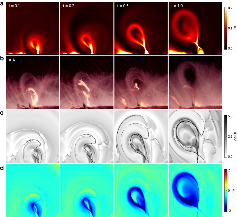
Figure 4: Temporal evolution of the eruptive structure in 2D view. (a) Distribution of current density on the vertical cross section (the $y=0$ plane). Here the current density is normalized by local magnetic field strength, which provides a high contrast of thin current layers with other volumetric currents. (b) SDO/AIA images of the X8.2 flare observed at the solar limb. The images are made by combination of two AIA channels 211 Å and 304 Å, and they are rotated to roughly match the direction of the simulated eruption. (c)-(d) Distributions of magnetic squashing degree $Q$ and twist number $T_{w}$, respectively, on the same cross section in (a).

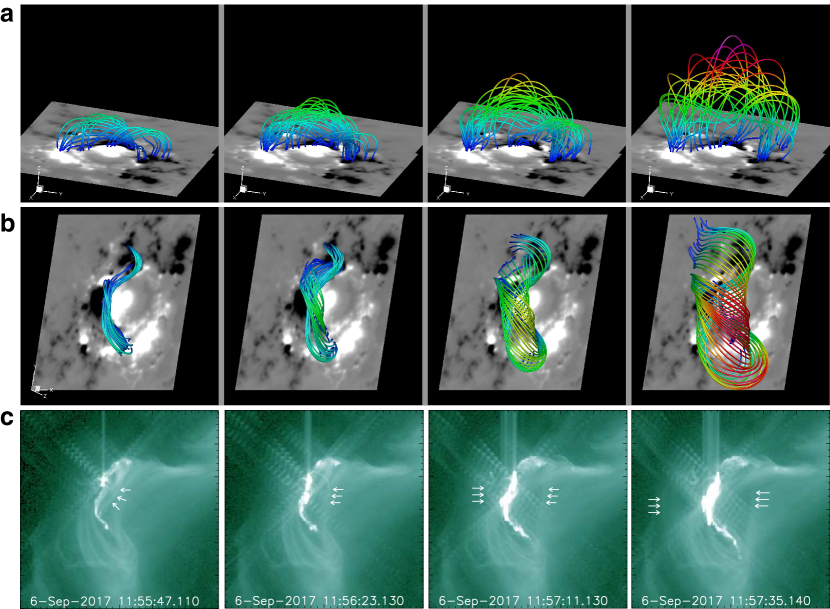
Figure 5: The eruptive structure in 3D and comparison with SDO/AIA observation. (a) Side view of sampled magnetic field lines of the erupting MFR. The magnetic field lines are false-colored by the value of height $z$ for a better visualization. The bottom surface is shown with the photospheric magnetogram. (b) Magnetic field lines that form the surface of the MFR (see Supplementary Movie 1 for a 3D rotation view of these field lines). The view angle is arranged to be the same as that of the SDO. (c) SDO/AIA 94 Å observations of the erupting process. Two sets of arrows mark the two expanding edges, presumably corresponding to the expanding surface of the MFR. Such expanding features can be seen more clearly in the Supplementary Movie 3.

The onset of the flare is characterized by a drastic rise and expansion of the MFR in the MHD simulation, which is shown in Fig. 4 for a vertical cross section and Fig. 5 for the 3D configuration. As clearly seen from the cross section of current density (Fig. 4a), there forms a narrow current layer of upside-down teardrop shape, which actually represents the closed boundary layer of the MFR. Such boundary is precisely depicted by the QSLs that separate the MFR with its surrounding flux, as shown in the map of magnetic squashing degree (Fig. 4c). Below the MFR, a more intense CS forms connecting the cusp of the teardrop to the bottom. Interestingly, there is an intersection of QSLs below the MFR, which forms an X shape of increasing height and size. Such intersection of QSLs is a magnetic null point configuration in the 2D plane, while in 3D it is a hyperbolic flux tube (HFT) ³⁶ which possesses the highest values of $Q$. Strong current density preferentially forms there and triggers reconnection. Indeed, the CS also evolves to an X shape since magnetic reconnection is triggered in the HFT, leaving another cusp connecting the bottom boundary.

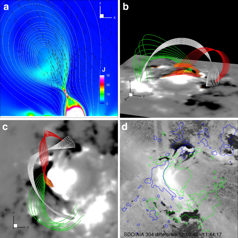
Figure 6: Illustration of the reconnection process below the rising MFR. (a) Current density distribution and plasma flows (denoted by arrows) on the vertical cross section (the $y=0$ plane) at time of $t=1.0$. The white lines are 2D field lines tracing on the plane. (b) 3D configuration of the reconnection. The white lines represent the main body of the MFR. The red and green lines represent the reconnecting field lines below the rope. Their inner footpoints are sheared past each along the PIL, and thus the field directions change abruptly across the CS, in which reconnection takes place, results in a long field line joining the MFR and a short arcade below which forms the post-flare loops (as shown by the yellow lines). The objects colored in red and orange are thin layers with strongest current density throughout the volume, showing the CS in 3D. (c) Top view of the same magnetic field lines shown in (b). (d) Difference of AIA 304 Å images of post-flare with pre-flare time showing two dimming sites (or transient coronal holes) that match the locations of the MFR legs. The contour lines are shown for $B_{z}=-500$ G (colored in blue) and $500$ G (colored in green).

The plasma flows near the CS are plotted in Fig. 6a, which shows a typical pattern of reconnection flow in 2D, i.e., inflows at two sides of the CS and outflows away from its two ends. This reconnection along with the cusp-CS-rope configuration (see the 2D field lines in Fig. 6a) reproduce nicely the picture of the standard flare model in 2D. Furthermore, the shape of enhanced current layer and its evolution look rather similar to the AIA images of the limb X8.2 flare of the same AR (Fig. 4b), which show a bright ring enclosing a relatively dark cavity of increasing size. The coronal cavity often indicates an MFR ²⁷, while its outer edge is bright because heating is enhanced there by the dissipation of the strong current in the boundary layer of rope. Below the cavity is an even brighter cusp connecting the solar surface, which is also matched by the simulation. Evolution of the magnetic twist distribution as shown in Fig. 4d indicates that the reconnection adds magnetic twist to the MFR ³⁷. The twist is added to the outer layer of the rope, while its center keeps the original value of the pre-flare configuration. The rising path of the MFR deviates from the vertical axis to the east side (the $-x$ direction), where the magnetic pressure is weaker than the west side (the $+x$ direction).

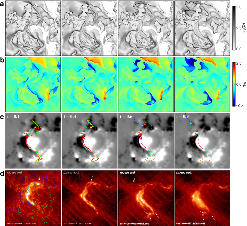
Figure 7: Structures and evolution at the bottom surface. (a) Magnetic squashing degrees. (b) Magnetic twist numbers. (c) Magnetic footpoints (color dots) of the field lines that are traced from the CS to the bottom surface. The colors represent the strength of local magnetic field, red for strong and blue for weak. (d) SDO/AIA 304 Å images of the flare ribbons. The arrows denote the two weak ribbons that form in the far-side polarities P1 and N1.

In 3D, the MFR’s surface (or boundary) is complex, but an arched tube structure can be seen from the QSLs (Supplementary Movie 1), within which the magnetic twist is distinctly stronger than that of the ambient flux (Supplementary Movie 2, Fig. 7a and b). With the rising of the MFR body, its conjugated legs are rooted in the far-side polarities P1/N1 without connection to P0/N0. Consequently, the initial elongated distribution of magnetic twist along the main PIL becomes coherent in the two feet of the rope, which expand in size with time (Supplementary Movie 4). Both feet are rather irregular: the south one forms closed rings while the north one is even more complex and is split into two fractions due to the mixed magnetic polarities there. As can be seen in Supplementary Movie 4, the south foot expands from the initial closed QSLs that separate the P1-N1 flux with other connections. Thus the initial P1-N1 flux provides a seed for the subsequent erupting rope, and the weakly twisted flux remains in the center of the rope. Evolution of the magnetic field lines traced on the surface of rope, which forms the tube-like QSLs, demonstrates the expansion of the rope in 3D (Fig. 5b). This expansion is also reflected in the observation of an EUV hot channel by SDO/AIA 94 Å. As observed from a nearly top view (see Fig. 5c), there are bright edges expanding from two sides of the flare ribbon (see also the Supplementary Movie 3), which agrees well with the expanding surface of the simulated rope (as seen in the same view angle, Fig. 5b). Such EUV hot channel is often associated with erupting MFR ³⁸; ³⁹, and here it is suggested to correspond specifically to the surface of MFR. There appears no writhe of the rope, as seen in both the simulation and the observation, indicating that the KI did not occur. Thus the TI is probably the driving mechanism of the eruption.

At the bottom surface, the QSL initially coinciding with the main PIL bifurcates in two parallel ones which depart from each other (see Fig. 7a and Supplementary Movie 4). This is due to the formation of the HFT below the MFR and the continuous reconnection in the corona. This reconnection in 3D occurs in a tether-cutting-like configuration (as illustrated in Fig. 6b and c), which cuts the connection of the twisted/sheared arcades at their inner footpoints with the photosphere. In observation, the feet of erupting MFR can be indicated by transient coronal dimming accompanied with eruptions, which is thought to be resulted by the plasma evacuation along the legs of the erupting MFR ⁴⁰; ⁴¹. In Fig. 6d, a time difference of 304 Å images before and after the eruption is plotted, which distinctly show two patches of coronal dimming in the polarities N1 and P1, respectively. These dimming sites coincide well with the two feet of the erupting MFR in the MHD model.

Our simulation reproduced the changing geometry of flare ribbons (Fig. 7), which correspond to the footpoints of magnetic field lines that are undergoing reconnection. These field lines, forming the surface of the MFR (or the tube-like QSLs), pass through the CS (or the HFT) below the rising rope. As can be seen in Fig. 7d and Supplementary Movie 5, there are two main flare ribbons (the brightest ones) along the main PIL, which exhibit a separation motion with time. The footpoints of reconnecting field lines match strikingly well the spatial location of the main double ribbons as well as their separation. In addition to the main double ribbons, there are relatively weak ribbons extending in the two far-side polarities, P1 and N1, as shown by the arrows in Fig 7d. It can be seen that these weak ribbons form a nearly closed ring in the south polarity, P1, while the north one is rather complex. These ribbons should be produced by reconnection-released energy reaching the far-end footpoints of the reconnecting field lines traced from the CS, which forms the boundaries of the MFR’s legs. With the separation of the main double ribbons, the closed region formed by the secondary ribbons also expands. This corresponds to the process of more and more flux joining in the MFR through the reconnection in the CS, which is basically in line with the 3D standard flare model. In Supplementary Fig. 1, the separation speed of the two main ribbons from the simulation is compared with that from observation: the modeled one is $50\sim 70$ km s^-1 which is approximately $3\sim 5$ times larger than the observed one ($10\sim 20$ km s^-1). The reconnection rate, as measured by the ratio of inflow speed to the local Alfvén speed (i.e., the inflow Alfvén Mach number), is $0.05\sim 0.1$ in the MHD simulation, which is comparable to the estimated values from direct observation analysis of different flares ⁴²; ⁴³. Thus, the real value of the reconnection rate for this X9.3 flare should be $0.01\sim 0.03$, if we apply the same scale factor, i.e., the ratio of the simulated ribbon separation speed with the observed one, to our simulated reconnection rate.

Finally, the modeled post-flare loops, which is the short magnetic arcades immediately below the flare CS, show a strong-to-weak transition of magnetic shear with the progress of the flare reconnection (Supplementary Fig. 2a). Such configuration evolution of flare loops is well observed for typical two-ribbon flares ¹⁰. Another well-documented fact we have reproduced (Supplementary Fig. 2b) is a permanent enhancement of the transverse field along the main PIL on the bottom surface after flare ⁴⁴.

Discussion

We have revealed the topological evolution of magnetic configuration associated with a solar flare through a combination of observation data and numerical simulation. Reconstruction of the coronal magnetic field immediately prior to the flare results in an MFR, which is a basic building block of the standard flare model. Much more complicated than any theoretical or idealized model, the MFR consists of multiple bundles of field lines with different connections and twist degrees. Owing to a strongly distorted, quadrupolar magnetic system as observed on the photosphere, the main body of the MFR forms a C shape. This is unlike a typically observed coronal sigmoid that is often associated with pre-flare MFR. Magnetic field lines of the MFR run horizontally over the strongly sheared PIL in the core of the AR. The bottom of the rope is attached on the photosphere, resulting in BPs along the PIL. Analysis of the decay index of the background potential field in the vicinity of the MFR shows that a major part of the MFR already enters into the TI domain.

The unstable nature of the pre-flare magnetic field results in fast expansion and rising of the MFR in the MHD simulation as initialized by the reconstruction data. In the wake of the rising MFR, an HFT comes into being, i.e., an intersection of the QSLs that warp the rope. Strong current density thus accumulates in the HFT, forming a CS and reconnection is consequently triggered there. Magnetic twist is sequentially built up on the outer layer of the rope through reconnection of the field lines there. The modeled magnetic configuration and evolution are found to be consistent with observed EUV features of the eruption, such as the expanding hot channels that are presumably the QSLs of the rope, the dark cavity with bright edge that corresponds to the cross section of the rope, and the coronal dimming in the feet of the rope. Most importantly, by tracing the newly-reconnected field lines from the CS to the bottom surface, we have reproduced the location of two main flare ribbons as well as their separation with time, which is achieved for the first time. Furthermore, the average reconnection rate of the flare could be estimated from the comparison of the simulated ribbon separation speed and the observed one. In addition to the main ribbons, there are relatively weak or secondary flare ribbons extending to the two feet of the rising rope, which actually correspond to the footpoints of the QSLs on the rope surface. The areas enclosed by these ribbons increase gradually as increasing amount of flux joins the MFR through the reconnection.

In summary, without any artificial assumption on the magnetic configuration, we reproduced the eruptive process of a great solar flare with numerical MHD simulation based directly on the observed magnetogram. The recreated flare process is found to be in correspondence with the standard flare model in 3D, thus providing the strong evidence supporting such a model.

Methods

Instrument and data. The SDO/AIA can provide a full-disk image of the Sun simultaneously in 6 EUV filters, including 171 Å, 193 Å, 211 Å, 335 Å, 94 Å, and 131 Å. The spatial resolutions of all these filters are $0.6$ arcsec and the cadences are 12 seconds. The vector magnetogram used for our coronal field extrapolation is taken by SDO/HMI ⁴⁵. In particular, we used the data product of the Space-weather HMI Active Region Patch (SHARP) ⁴⁶, which has resolved the 180^∘ ambiguity by using the minimum energy method, modified the coordinate system via the Lambert method and corrected the projection effect. Furthermore, this flare was associated with an erupting filament. For checking the location of the filament, the H$\alpha$ data, with spatial resolution of 1 arcsec and cadence of 1 minute, from Global Oscillation Network Group (GONG) are used as well.

All the data used in current study are publicly available: the SDO/HMI vector magnetograms and SDO/AIA images can be downloaded from the Joint Science Operations Center (JSOC) website http://jsoc.stanford.edu/; the GONG data can be downloaded from https://gong2.nso.edu/.

Coronal Magnetic Field Reconstruction. The pre-flare coronal magnetic field is extrapolated by the CESE–MHD–NLFFF code ³². It belongs to the class of magneto-frictional methods ⁴⁷ that seek nonlinear force-free equilibrium

$$(\nabla\times{\mathbf{B}})\times{\mathbf{B}}={\mathbf{0}}$$ (1)

for given boundary value of observed vector magnetograms. It solves a set of modified zero-$\beta$ MHD equations with a friction force using an advanced conservation-element/solution-element (CESE) space-time scheme on a non-uniform grid with parallel computing ⁴⁸. Starting from a potential field extrapolated from the vertical component of the vector magnetogram, the MHD system is driven to evolve by incrementally changing the transverse field at the bottom boundary to match the vector magnetogram, after which the system will be relaxed to a new equilibrium. The code has an option of using adaptive mesh refinement and multi-grid algorithm for optimizing the relaxation process. The computational accuracy is further improved by a magnetic-field splitting method, in which the total magnetic field is divided into a potential-field part and a non-potential-field part and only the latter is actually solved in the MHD system. Before inputting to the code, the vector magnetograms are usually required to be preprocessed to reduce the Lorentz force involved. Furthermore, to be consistent with the code, we developed a unique preprocessing method ⁴⁹ that also splits the vector magnetogram into a potential part and a non-potential part and handles them separately. Then the non-potential part is modified and smoothed by an optimization method ⁵⁰ to fulfill the conditions of total magnetic force-freeness and torque-freeness. Details of the code are described in a series of papers ⁵¹; ⁵²; ⁵³. It is well tested by different benchmarks including a series of analytic force-free solutions ⁵⁴ and numerical MFR models ⁵⁵; ⁵⁶, and have been applied to the SDO/HMI vector magnetograms ³²; ⁵³, which enable to reproduce magnetic configurations in very good agreement with corresponding observable features, including coronal loops, filaments, and sigmoids.

MHD Model. The MHD simulation is realized by solving the full set of 3D, time-dependent ideal MHD equations with solar gravity ⁵⁷. The initial condition consists of magnetic field provided by the NLFFF model and a hydrostatic plasma. The initial temperature is uniform, with a value typically in the corona, $T=10^{6}$ K (sound speed $c_{S}=128$ km s^-1). The initial plasma density is uniform in horizontal direction and vertically stratified by the gravity. To mimic the coronal low-$\beta$ and highly tenuous conditions, the plasma density is configured to make the plasma $\beta$ less than $0.1$ in most of the computational volume. The smallest value of $\beta$ is $5\times 10^{-4}$, corresponding to the largest Alfvén speed $v_{\rm A}$ of approximately 8 Mm s^-1. The units of length and time in the model are $L=11.5$ Mm (approximately 16 arcsec on the Sun) and $\tau=L/c_{S}=90$ s, respectively. The MHD solver is the same CESE code described in ref⁴⁸. We use a non-uniform grid adaptively based on the spatial distribution of the magnetic field and current density in the NLFFF model. This grid is designed for the sake of saving computational resources without losing numerical accuracy, and more details of this can be found in ref ⁵⁸. The smallest grid is $\Delta x=\Delta y=2\Delta z=0.36$ Mm (approximately 0.5 arcsec on the Sun). A moderate viscosity $\nu$, which corresponds to Reynolds number $R_{e}=Lv_{\rm A}/\nu$ of $\sim 10^{2}$, is used to keep the numerical stability of the code running for the whole duration of the flare eruption process. No explicit resistivity is included in the magnetic induction equation, and magnetic reconnection is still allowed due to numerical resistivity $\eta$, which corresponds to Lundquist number (or magnetic Reynolds number) of $S=Lv_{\rm A}/\eta$ of $\sim 5\times 10^{3}$. Although there is no doubt that the viscosity and numerical resistivity in our model overestimate the real values in the coronal plasma (which are on the order of $10^{8}\sim 10^{10}$), the basic magnetic topological evolution as simulated is still robust ⁵⁷. The simulation is stopped before any disturbance reaches the numerical boundaries. At the bottom boundary (i.e., the coronal base), all the variables are fixed except the transverse components of the magnetic field, which are specified by linear extrapolation from the two adjacent inner points along the $z$-axis.

In the combination of NLFFF model and MHD simulation, one should note almost all the available NLFFF codes actually generate non-force-free magnetic field data with residual Lorentz force that is often non-negligible. This is indicated by the misalignment of the electric current ${\mathbf{J}}$ and magnetic field vector ${\mathbf{B}}$ ⁵⁹, which is usually measured by CWsin, a current-weighted sine of the angle between ${\mathbf{J}}$ and ${\mathbf{B}}$. CWsin is typically in the range of $0.2$ to $0.4$ ⁶⁰; ⁶¹; ⁶². Another metric $E_{{\bf\nabla}\times{\mathbf{B}}}$ measuring more directly the residual Lorentz force is defined as the average ratio of the force to the sum of the magnitudes of magnetic tension and pressure forces ⁶³. In the studied event here, these two metrics for the CESE–MHD–NLFFF extrapolation are respectively, CWsin $=0.23$ and $E_{{\bf\nabla}\times{\mathbf{B}}}=0.17$ in the strong current region. These metrics are reasonably small as compared with other codes (e.g., see the last column of Table 2 in ref ⁶²), but such residual force can instantly induce plasma motions in a low-$\beta$ and highly tenuous plasma environment. This motion provides a way of perturbing the system. If the system is significantly far away from unstable, such unbalance state will relax to a new MHD equilibrium as the induced motion can alter the magnetic field, which in turn generates restoring Lorentz force to stabilize the system. Else if the system is unstable or not far away from unstable regime, the perturbation could grow and lead to a drastic evolution of the system as driven by the instability. Thus the combination of NLFFF and MHD model can be used to test the potentially unstable nature or instability of NLFFF. Although such combination of NLFFF and MHD models might not be able to identify the true mechanism triggering flare, it still provides a viable tool to reproduce the fast magnetic evolution during the flare.

Magnetic field analysis tools. A set of magnetic field analysis methods is used in this study, including search of BPs, calculation of magnetic twist number, squashing degree and decay index, which are described in the following.

BPs are places on photospheric PIL where the transverse field directs from the negative polarity to positive one. This is inverse to a normal case that transverse field directs from positive flux to negative one, and thus the field line is concave upward. BPs can be located by searching the point on the magnetogram where the conditions

$${\mathbf{B}}\cdot\nabla B_{z}>0,\ \ B_{z}=0$$ (2)

are satisfied. Magnetic dips are searched using the same conditions but applied for the full 3D volume of the field.

The magnetic twist number $T_{w}$ for a given (closed) field line is defined by ³⁴

$$T_{w}=\int_{L}\frac{(\nabla\times{\mathbf{B}})\cdot{\mathbf{B}}}{4\pi B^{2}}dl$$ (3)

where the integral is taken along the length $L$ of the magnetic field line from one footpoint to the other.

The squashing degree $Q$ is derived based on the mapping of two footpoints for a field line. Specifically, a field line starts at one footpoint $(x,y)$ and ends at the other footpoint $(X(x,y),Y(x,y))$. Then the squashing degree associate with this field line is given by ³⁶

$$Q=\frac{a^{2}+b^{2}+c^{2}+d^{2}}{|ad-bc|}$$ (4)

where

$$a=\frac{\partial X}{\partial x},\ \ b=\frac{\partial X}{\partial y},\ \ c=\frac{\partial Y}{\partial x},\ \ d=\frac{\partial Y}{\partial y}.$$ (5)

Usually QSLs can be defined as locations where $Q>>2$.

In the torus instability (TI) ¹⁷, which is a result of the loss of balance between the “hoop force” of the rope itself and the “strapping force” of the ambient field, the decay index $n$ plays a key role. It quantifies the decreasing speed of the strapping force along the distance from the torus center. Here $n$ is calculated in the vertical cross section perpendicularly crossing the main axis of the rope (see Fig. 3c) in such manner: we regard the bottom PIL point, named O (denoted by the black circle in the figure) as the center of the torus, and for a given grid point P, $n({\rm P})=-d\log(B_{\rm p})/d\log(h)$, where $B_{\rm p}$ is the magnetic field component perpendicular to the direction vector ${\mathbf{r}}_{\rm OP}$, and $h=|{\mathbf{r}}_{\rm OP}|$. Here the strapping field is approximated by the potential field model that matches the $B_{z}$ component of the photospheric magnetogram ⁹; ⁵¹.

Acknowledgments

Data from observations are courtesy of NASA SDO/AIA and the HMI science teams. The computation work was carried out on TianHe-1 (A) at the National Supercomputer Center in Tianjin, China. This work is supported by the National Natural Science Foundation of China (41574170, 41574171, 41531073, 41731067). C.J. and Q.H. acknowledge NSF grant AGS-1650854 for partial support.

Author contribution

C.J. developed the model, performed the result analysis and wrote the first draft. P.Z. performed part of the observation analysis. All authors participated in discussions and revisions on the manuscript.

Competing financial interests:

The authors declare no competing financial interests.

Supplementary information

Supplementary Fig 1 and Movies 1–5 are accompanied with this paper.

Supplementary Movie 1: Rotating view of 3D structure of the QSLs that warp the erupting MFR at simulation time $t=1$. (a) The iso-surface of $Q=1000$, (b) Sampled magnetic field lines that form the QSLs. The colors denote the value of height $z$.

Supplementary Movie 2: Slice through the volume showing the squashing degree $Q$ (a) and the magnetic twist degree $T_{w}$ (b).

Supplementary Movie 3: Observation of the flare eruption in SDO/AIA 94 Å.

Supplementary Movie 4: Temporal evolution of the magnetic squashing degree (a) and twist degree (b) on the bottom surface.

Supplementary Movie 5: Observation of the evolution of flare ribbons in SDO/AIA 304 Å.

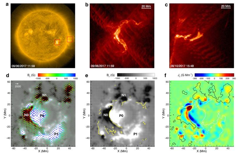
Figure 1: The flare location and photospheric magnetic field. (a) Full-disk image of the Sun observed in SDO/AIA 171 Å. The two boxes indicate the locations of the on-disk X9.3 flare on September 6 and the limb X8.2 flare occurred on September 10. (b)-(c) SDO/AIA 304 Å image of the X9.3 flare and the X8.2 flare, respectively. (d)-(f) SDO/HMI vector magnetogram taken at 11:36 UT on September 6, which is 17 min before the X9.3 flare onset. In (d), the magnetic flux distribution, i.e., $B_{z}$, is overlaid by the transverse field vector $(B_{x},B_{y})$ as denoted by the colored arrows. The main magnetic polarities P0, N0, P1, and N1 are labeled. In (e) the yellow curves are the BP locations along the PIL. (f) Distribution of the vertical current density, which is defined as $J_{z}=\partial_{x}B_{y}-\partial_{y}B_{x}$. The contour lines are plotted for $B_{z}=-500$ G (colored as black) and 500 G (white). The ratio of the direct current (DC) to the return current (RC) for the positive flux is $|{\rm DC}/{\rm RC}|^{+}=2.31$, and for the negative flux is $|{\rm DC}/{\rm RC}|^{-}=2.26$.

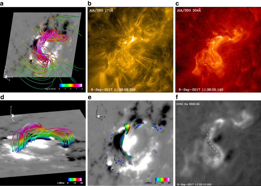
Figure 2: Comparison of the reconstructed magnetic field with the observed features of the solar corona prior to the flare. (a) SDO view of sampled magnetic field lines of the NLFFF reconstruction. The color of the lines represents the value of current density $J$ (normalized by its average value $J_{\rm ave}$ in the computational volume). The background is the photospheric magnetogram. (b) and (c) SDO/AIA 171 Å and 304 Å images of the pre-flare corona. (d) The low-lying magnetic field lines in the core region. The field lines are color-coded by the value of height $z$. (e) Locations of dips in the magnetic field lines, and the color indicates the value of height $z$. (f) GONG H$\alpha$ image of the AR. The dashed curve denotes the location of a long filament.

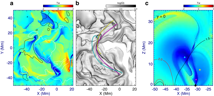
Figure 3: Detailed configuration of the reconstructed pre-flare magnetic field. (a) Map of magnetic twist number $T_{w}$ at the bottom surface $z=0$. Overlaid are contour lines for $B_{z}=500$ G (white) and 500 G (black). (b) Map of magnetic squashing factor $Q$ at the bottom. The black thin lines as formed by the large-$Q$ value are locations of magnetic topology separatries and QSLs where the magnetic field-line mapping is discontinuous or steeply changes. Three field lines with different colors are plotted to represent the magnetic flux of different connections, which make up the MFR. (c) Twist number distribution on a vertical cross section ($y=0$). The three colored stars denote the intersection points of the sample field lines shown in (b) with the cross section. The black circle indicates the main PIL. The contour lines are shown for the decay index $n=1.5$ and 2 (see Methods).

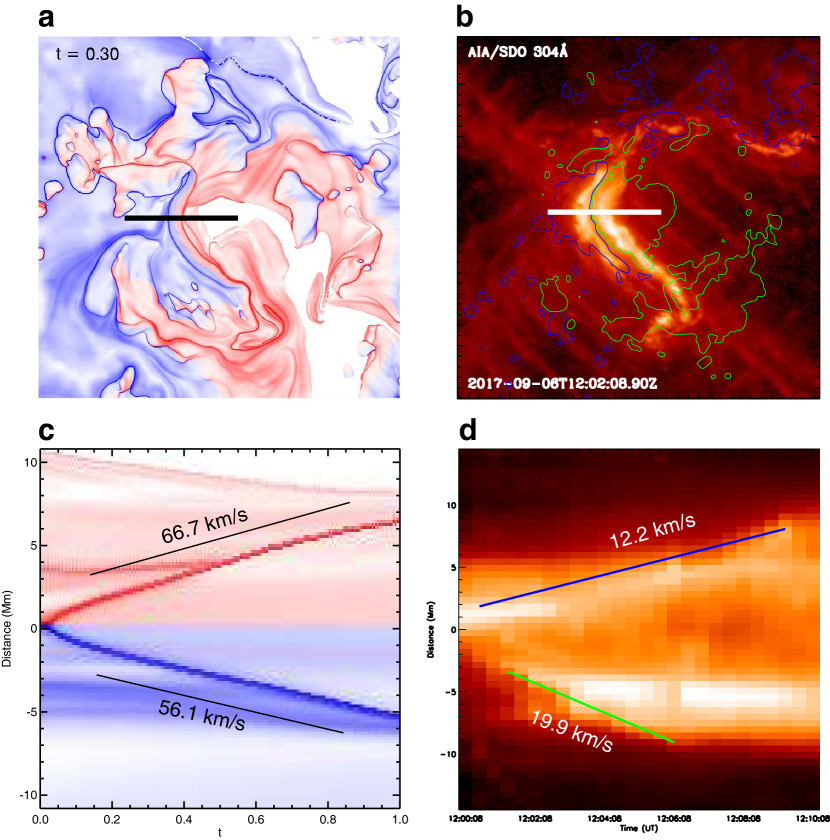
Supplementary Fig 1: Comparison of flare-ribbon separation speed from MHD simulation and that from observation. (a) The QSL map on the bottom at time of $t=0.3$. The black line segment denotes the location where a time sequence of stack is plotted in (c) for tracking the separation of the main QSLs that maps the reconnection footpoint. (b) SDO/AIA 304 Å image of the flare ribbons. In the same way, the white line segment is the location of the time stack shown in (d), which shows the separation motion of the main flare ribbons. The lines shown in (c) and (d) represent approximately the speeds of the ribbons with time, respectively.

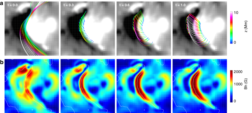
Supplementary Fig 2: Strong-to-weak shear transition in post-flare loops and enhancement of horizontal field. (a) The closed magnetic arcades immediately below the reconnection site. Note that initially ($t=0$) they are long field lines that form the pre-flare MFR. The colors of the lines denote the value of height $z$. The background is shown with $B_{z}$ on the bottom. (b) Distribution of the horizontal field $B_{h}=\sqrt{B_{x}^{2}+B_{y}^{2}}$ on the bottom. The PIL of the magnetic flux $B_{z}$ is shown by the white-colored lines.

References

- 1 B. Schmieder, P. Démoulin, and G. Aulanier. Solar filament eruptions and their physical role in triggering coronal mass ejections. Advances in Space Research, (0):–, 2013.
- 2 M. J. Aschwanden. Physics of the Solar Corona. An Introduction. Praxis Publishing Ltd, August 2004.
- 3 E. R. Priest and T. G. Forbes. The magnetic nature of solar flares. Astron. Astrophys. Rev., 10:313–377, 2002.
- 4 K. Shibata and T. Magara. Solar Flares: Magnetohydrodynamic Processes. Living Reviews in Solar Physics, 8:6, December 2011.
- 5 H. Carmichael. A Process for Flares. NASA Special Publication, 50:451, 1964.
- 6 P. A. Sturrock. Model of the High-Energy Phase of Solar Flares. Nature, 211:695–697, August 1966.
- 7 T. Hirayama. Theoretical Model of Flares and Prominences. I: Evaporating Flare Model. Solar Phys., 34:323–338, February 1974.
- 8 R. A. Kopp and G. W. Pneuman. Magnetic reconnection in the corona and the loop prominence phenomenon. Solar Phys., 50:85–98, October 1976.
- 9 G. Aulanier, T. Török, P. Démoulin, and E. E. DeLuca. Formation of Torus-Unstable Flux Ropes and Electric Currents in Erupting Sigmoids. Astrophys. J., 708:314–333, January 2010.
- 10 G. Aulanier, M. Janvier, and B. Schmieder. The standard flare model in three dimensions. I. Strong-to-weak shear transition in post-flare loops. Astron. Astrophys., 543:A110, July 2012.
- 11 M. Janvier, G. Aulanier, V. Bommier, B. Schmieder, P. D?moulin, and E. Pariat. Electric currents in flare ribbons: Observations and three-dimensional standard model. The Astrophysical Journal, 788(1):60, 2014.
- 12 M. Janvier, G. Aulanier, and P. Démoulin. From Coronal Observations to MHD Simulations, the Building Blocks for 3D Models of Solar Flares (Invited Review). Solar Phys., 290:3425–3456, December 2015.
- 13 A. W. Hood and E. R. Priest. Critical conditions for magnetic instabilities in force-free coronal loops. Geophysical and Astrophysical Fluid Dynamics, 17:297–318, 1981.
- 14 T. Török, B. Kliem, and V. S. Titov. Ideal kink instability of a magnetic loop equilibrium. Astron. Astrophys., 413:L27–L30, January 2004.
- 15 Y. Fan and S. E. Gibson. The Emergence of a Twisted Magnetic Flux Tube into a Preexisting Coronal Arcade. Astrophys. J. Lett., 589:L105–L108, June 2003.
- 16 G. Bateman. MHD instabilities. 1978.
- 17 B. Kliem and T. Török. Torus Instability. Physical Review Letters, 96(25):255002, June 2006.
- 18 R. L. Moore and A. C. Sterling. Initiation of Coronal Mass Ejections. Washington DC American Geophysical Union Geophysical Monograph Series, 165:43, October 2006.
- 19 S. Yang, J. Zhang, X. Zhu, and Q. Song. Block-induced Complex Structures Building the Flare-productive Solar Active Region 12673. Astrophys. J. Lett., 849:L21, November 2017.
- 20 X. Sun and A. A. Norton. Super-flaring Active Region 12673 Has One of the Fastest Magnetic Flux Emergence Ever Observed. Research Notes of the American Astronomical Society, 1:24, December 2017.
- 21 H. P. Warren, D. H. Brooks, I. Ugarte-Urra, J. W. Reep, N. A. Crump, and G. A. Doschek. Spectroscopic Observations of Current Sheet Formation and Evolution. ArXiv e-prints, November 2017.
- 22 X. L. Yan, J. C. Wang, G. M. Pan, D. F. Kong, Z. K. Xue, L. H. Yang, and Q. L. Li. Successive X-class flares and coronal mass ejections driven by shearing motion and sunspot rotation in active region NOAA 12673. ArXiv e-prints, January 2018.
- 23 Y. Li, J. C. Xue, M. D. Ding, X. Cheng, Y. Su, L. Feng, J. Hong, H. Li, and W. Q. Gan. Spectroscopic Observations of a Current Sheet in a Solar Flare. ArXiv e-prints, January 2018.
- 24 Haimin Wang, Vasyl Yurchyshyn, Chang Liu, Kwangsu Ahn, Shin Toriumi, and Wenda Cao. Strong transverse photosphere magnetic fields and twist in light bridge dividing delta sunspot of active region 12673. Research Notes of the AAS, 2(1):8, 2018.
- 25 Nengyi Huang, Yan Xu, and Haimin Wang. Relationship between intensity of white-light flares and proton flux of solar energetic particles. Research Notes of the AAS, 2(1):7, 2018.
- 26 V. S. Titov, E. R. Priest, and P. Demoulin. Conditions for the appearance of ”bald patches” at the solar surface. Astron. Astrophys., 276:564, September 1993.
- 27 S. E. Gibson and Y. Fan. Coronal Prominence Structure and Dynamics: A Magnetic Flux Rope Interpretation. J. Geophys. Res., 111:A12103, 2006.
- 28 X. Sun, M. G. Bobra, J. T. Hoeksema, Y. Liu, Y. Li, C. Shen, S. Couvidat, A. A. Norton, and G. H. Fisher. Why is the great solar active region 12192 flare-rich but cme-poor? Astrophys. J. Lett., 804(2):L28, 2015.
- 29 Y. Liu, X. Sun, T. Török, V. S. Titov, and J. E. Leake. Electric-current Neutralization, Magnetic Shear, and Eruptive Activity in Solar Active Regions. Astrophys. J. Lett., 846:L6, September 2017.
- 30 I. Kontogiannis, M. K. Georgoulis, S.-H. Park, and J. A. Guerra. Non-neutralized Electric Currents in Solar Active Regions and Flare Productivity. Solar Physics, 292:159, November 2017.
- 31 T. Wiegelmann. Nonlinear force-free modeling of the solar coronal magnetic field. Journal of Geophysical Research (Space Physics), 113:3, March 2008.
- 32 C. Jiang and X. Feng. Extrapolation of the Solar Coronal Magnetic Field from SDO/HMI Magnetogram by a CESE-MHD-NLFFF Code. Astrophys. J., 769:144, June 2013.
- 33 S. Inoue, K. Kusano, T. Magara, D. Shiota, and T. T. Yamamoto. Twist and Connectivity of Magnetic Field Lines in the Solar Active Region NOAA 10930. Astrophys. J., 738:161, September 2011.
- 34 Rui Liu, Bernhard Kliem, Viacheslav S. Titov, Jun Chen, Yuming Wang, Haimin Wang, Chang Liu, Yan Xu, and Thomas Wiegelmann. Structure, stability, and evolution of magnetic flux ropes from the perspective of magnetic twist. The Astrophysical Journal, 818(2):148, 2016.
- 35 P. Demoulin, J. C. Henoux, E. R. Priest, and C. H. Mandrini. Quasi-Separatrix layers in solar flares. I. Method. Astron. Astrophys., 308:643–655, April 1996.
- 36 V. S. Titov, G. Hornig, and P. Démoulin. Theory of magnetic connectivity in the solar corona. J. Geophys. Res., 107:1164, August 2002.
- 37 W. Wang, R. Liu, Y. Wang, Q. Hu, C. Shen, C. Jiang, and C. Zhu. Buildup of a highly twisted magnetic flux rope during a solar eruption. Nature Communications, 8:1330, November 2017.
- 38 J. Zhang, X. Cheng, and M.-D. Ding. Observation of an evolving magnetic flux rope before and during a solar eruption. Nature Communications, 3:747, March 2012.
- 39 X. Cheng, J. Zhang, S. H. Saar, and M. D. Ding. Differential Emission Measure Analysis of Multiple Structural Components of Coronal Mass Ejections in the Inner Corona. Astrophys. J., 761:62, December 2012.
- 40 J. Qiu, Q. Hu, T. A. Howard, and V. B. Yurchyshyn. On the Magnetic Flux Budget in Low-Corona Magnetic Reconnection and Interplanetary Coronal Mass Ejections. Astrophys. J., 659:758–772, April 2007.
- 41 D. F. Webb, R. P. Lepping, L. F. Burlaga, C. E. DeForest, D. E. Larson, S. F. Martin, S. P. Plunkett, and D. M. Rust. The origin and development of the May 1997 magnetic cloud. J. Geophys. Res., 105:27251–27260, December 2000.
- 42 Y. Su, A. M. Veronig, G. D. Holman, B. R. Dennis, T. Wang, M. Temmer, and W. Gan. Imaging coronal magnetic-field reconnection in a solar flare. Nature Physics, 9:489–493, August 2013.
- 43 J. Q. Sun, X. Cheng, M. D. Ding, Y. Guo, E. R. Priest, C. E. Parnell, S. J. Edwards, J. Zhang, P. F. Chen, and C. Fang. Extreme ultraviolet imaging of three-dimensional magnetic reconnection in a solar eruption. Nature Communications, 6:7598, June 2015.
- 44 H. Wang and C. Liu. Circular Ribbon Flares and Homologous Jets. Astrophys. J., 760:101, December 2012.
- 45 J. Schou, P. H. Scherrer, R. I. Bush, R. Wachter, S. Couvidat, M. C. Rabello-Soares, R. S. Bogart, J. T. Hoeksema, Y. Liu, T. L. Duvall, D. J. Akin, B. A. Allard, J. W. Miles, R. Rairden, R. A. Shine, T. D. Tarbell, A. M. Title, C. J. Wolfson, D. F. Elmore, A. A. Norton, and S. Tomczyk. Design and Ground Calibration of the Helioseismic and Magnetic Imager (HMI) Instrument on the Solar Dynamics Observatory (SDO). Solar Phys., 275:229–259, January 2012.
- 46 M. G. Bobra, X. Sun, J. T. Hoeksema, M. Turmon, Y. Liu, K. Hayashi, G. Barnes, and K. D. Leka. The Helioseismic and Magnetic Imager (HMI) Vector Magnetic Field Pipeline: SHARPs - Space-Weather HMI Active Region Patches. Solar Phys., 289:3549–3578, September 2014.
- 47 G. Roumeliotis. The “Stress-and-Relax” Method for Reconstructing the Coronal Magnetic Field from Vector Magnetograph Data. Astrophys. J., 473:1095–+, December 1996.
- 48 C. W Jiang, X. S. Feng, J. Zhang, and D. K. Zhong. AMR Simulations of Magnetohydrodynamic Problems by the CESE Method in Curvilinear Coordinates. Solar Phys., 267:463–491, 2010.
- 49 C. Jiang and X. Feng. Preprocessing the Photospheric Vector Magnetograms for an NLFFF Extrapolation Using a Potential-Field Model and an Optimization Method. Solar Phys., 289:63–77, January 2014.
- 50 T. Wiegelmann and T. Neukirch. An optimization principle for the computation of MHD equilibria in the solar corona. Astron. Astrophys., 457:1053–1058, October 2006.
- 51 C. W. Jiang, X. S. Feng, S. T. Wu, and Q. Hu. Magnetohydrodynamic simulation of a sigmoid eruption of active region 11283. Astrophys. J. Lett., 771(2):L30, 2013.
- 52 C. W. Jiang, S. T. Wu, X. S. Feng, and Q. Hu. Formation and eruption of an active region sigmoid. i. a study by nonlinear force-free field modeling. Astrophys. J., 780(1):55, 2014.
- 53 C. Jiang, S. T. Wu, X. Feng, and Q. Hu. Nonlinear Force-free Field Extrapolation of a Coronal Magnetic Flux Rope Supporting a Large-scale Solar Filament from a Photospheric Vector Magnetogram. Astrophys. J. Lett., 786:L16, May 2014.
- 54 B. C. Low and Y. Q. Lou. Modeling solar force-free magnetic fields. Astrophys. J., 352:343–352, March 1990.
- 55 V. S. Titov and P. Démoulin. Basic topology of twisted magnetic configurations in solar flares. Astron. Astrophys., 351:707–720, November 1999.
- 56 A. A. van Ballegooijen. Observations and Modeling of a Filament on the Sun. Astrophys. J., 612:519–529, September 2004.
- 57 C. W. Jiang, S. T. Wu, X. S. Feng, and Q. Hu. Data-driven mhd simulation of a flux-emerging active region leading to solar eruption. Nature Comm., 7:11522, 2016.
- 58 C. Jiang, X. Yan, X. Feng, A. Duan, Q. Hu, P. Zuo, and Y. Wang. Reconstruction of a Large-scale Pre-flare Coronal Current Sheet Associated with a Homologous X-shaped Flare. Astrophys. J., 850:8, November 2017.
- 59 C. J. Schrijver, M. L. De Rosa, T. R. Metcalf, Y. Liu, J. McTiernan, S. Régnier, G. Valori, M. S. Wheatland, and T. Wiegelmann. Nonlinear Force-Free Modeling of Coronal Magnetic Fields Part I: A Quantitative Comparison of Methods. Solar Phys., 235:161–190, May 2006.
- 60 C. J. Schrijver, M. L. DeRosa, T. Metcalf, G. Barnes, B. Lites, T. Tarbell, J. McTiernan, G. Valori, T. Wiegelmann, M. S. Wheatland, T. Amari, G. Aulanier, P. Démoulin, M. Fuhrmann, K. Kusano, S. Régnier, and J. K. Thalmann. Nonlinear Force-free Field Modeling of a Solar Active Region around the Time of a Major Flare and Coronal Mass Ejection. Astrophys. J., 675:1637–1644, March 2008.
- 61 M. L. DeRosa, C. J. Schrijver, G. Barnes, K. D. Leka, B. W. Lites, M. J. Aschwanden, T. Amari, A. Canou, J. M. McTiernan, S. Régnier, J. K. Thalmann, G. Valori, M. S. Wheatland, T. Wiegelmann, M. C. M. Cheung, P. A. Conlon, M. Fuhrmann, B. Inhester, and T. Tadesse. A Critical Assessment of Nonlinear Force-Free Field Modeling of the Solar Corona for Active Region 10953. Astrophys. J., 696:1780–1791, May 2009.
- 62 M. L. DeRosa, M. S. Wheatland, K. D. Leka, G. Barnes, T. Amari, A. Canou, S. A. Gilchrist, J. K. Thalmann, G. Valori, T. Wiegelmann, C. J. Schrijver, A. Malanushenko, X. Sun, and S. Régnier. The Influence of Spatial resolution on Nonlinear Force-free Modeling. Astrophys. J., 811:107, October 2015.
- 63 Aiying Duan, Chaowei Jiang, Qiang Hu, Huai Zhang, G. Allen Gary, S. T. Wu, and Jinbin Cao. Comparison of two coronal magnetic field models to reconstruct a sigmoidal solar active region with coronal loops. The Astrophysical Journal, 842(2):119, 2017.