Memory-induced complex contagion in epidemic spreading

Abstract

Albeit epidemic models have evolved into powerful predictive tools for the spread of diseases and opinions, most assume memoryless agents and independent transmission channels. We develop an infection mechanism that is endowed with memory of past exposures and simultaneously incorporates the joint effect of multiple infectious sources. Analytic equations and simulations of the susceptible-infected-susceptible model in unstructured substrates reveal the emergence of an additional phase that separates the usual healthy and endemic ones. This intermediate phase shows fundamentally distinct characteristics, and the system exhibits either excitability or an exotic variant of bistability. Moreover, the transition to endemicity presents hybrid aspects. These features are the product of an intricate balance between two memory modes and indicate that non-Markovian effects significantly alter the properties of spreading processes.

I Introduction

Epidemic modeling has proven to be a powerful tool for the study of contagion phenomena in biological, social, and technological systems, e.g., diseases, opinions, rumors and innovation Anderson and May (1991); Pastor-Satorras and Vespignani (2001); Bond et al. (2012). Variations of the benchmark susceptible-infected-susceptible (SIS) and susceptible-infected-recovered (SIR) models have provided valuable insights into the nature of spreading mechanisms, the dynamics of outbreaks, and the viability of containment protocols Colizza et al. (2007); Vespignani (2012); Pastor-Satorras et al. (2015). The inclusion of real-life contact and mobility patterns has yielded astonishingly accurate results, prompting the use of epidemic models as real-time predictive tools Colizza et al. (2006); Balcan et al. (2009); Tizzoni et al. (2012).

The canonical modeling scheme for contact-based contagion Anderson and May (1991); Pastor-Satorras et al. (2015) assumes Markov processes and isolated transmissions. Markov processes are memoryless, which translates into exponentially distributed interevent times and enhances the mathematical tractability. The inappropriateness of this approximation, however, is widely supported by empirical evidence, such as the peaked distributions of infection periods of numerous diseases Streftaris and Gibson (2012); Chowell and Nishiura (2014) or the bursty human activity patterns in social networks, well described by heavy-tailed distributions Oliveira and Barabasi (2005); González et al. (2008). On the other hand, assuming isolated transmissions leads to infection channels that are not influenced by their local environment. Consequently, the infection likelihood can be written as the sum of statistically independent exposures. Nevertheless, there is evidence supporting the existence of more complex, nondyadic mechanisms, e.g., in fungal and bacterial pathogen colonization Ben-Jacob et al. (1994); Donabedian (2003), and social contagion Castellano et al. (2009); Centola (2010); Hodas and Lerman (2014).

In recent years, an important amount of research has focused on overcoming these modeling limitations. Regarding memory, a wide array of modifications has been analyzed, such as two-step infection models Choi et al. (2017a, b), nonexponential distributions Van Mieghem and van de Bovenkamp (2013); Kiss et al. (2015); Starnini et al. (2017), and time-varying transmission probabilities Dodds and Watts (2004); Lü et al. (2011). Conversely, a plethora of complex contagion schemes has been proposed to mediate the assumption of independent transmissions. Examples include correlated, nonlinear transmission channels Liu et al. (1987); Boguñá et al. (2014), extended neighborhood effects Pérez-Reche et al. (2011); Gómez-Gardeñes et al. (2016), and deterministic threshold models Watts (2002); Centola et al. (2007). So far, not much research has focused on tackling both assumptions simultaneously, and little is know about how these two features interact. Such a combined approach is of particular interest for contagion phenomena that include a social component, such as awareness and vaccination campaigns Granell et al. (2013); Fu et al. (2017), or the spread of noncommunicable diseases (e.g., obesity, anxiety, and substance abuse) Christakis and Fowler (2007, 2008).

In this work, we develop an infection mechanism that is equipped with memory of past exposures to multiple infectious sources. A notion of social reinforcement/inhibition arises organically, and the concepts of non-Markovian dynamics and complex contagion become intrinsically coupled. We obtain analytic results for the SIS model and perform extensive stochastic simulations in random degree-regular networks. Our analysis reveals a sophisticated interplay between two memory modes, displayed by a collective memory loss and the dislocation of the critical point into two phase transitions. An intermediate region emerges where the system is either excitable or bistable, exhibiting fundamentally distinct behaviors compared to the typical healthy and endemic phases. Additionally, the transition to the endemic phase becomes hybrid, showing both continuous and discontinuous properties.

II miccSIS model

Epidemic-like models are employed for a variety of dynamics, such as opinion formation, rumor spreading, and innovation adoption. Although we use the original disease-specific terminology throughout this work, the scope of our analysis extends to all of these fields.

II.1 General framework

The memory-induced complex contagion susceptible-infected-susceptible (miccSIS) model describes a population of agents that can be either susceptible (healthy) or infected (infectious), and is embedded on an undirected, unweighted network. The contact network is encoded in the adjacency matrix, which is nonspatial (it carries no information about the agents’ physical position) and static (it remains fixed over time).

Infected nodes have a constant infectivity rate, $\upsilon$, and continuously spread doses of contagion towards their entire neighborhood. They target all of their neighbors equally, transmitting pathogen along each edge at constant rate $\upsilon$. Susceptible nodes collect these toxins from all their neighbors, amassing a total viral load $\kappa$, and transition to the infected state with probability ${\psi^{*}_{\text{inf}}(\kappa)\text{d}\kappa}$, where ${\psi^{*}_{\text{inf}}(\kappa)}$ is the infection probability density. Infected nodes are unaffected by the toxins (their viral load does not increase) and recover spontaneously after a random time $t$, with interevent time distribution ${\psi_{\text{rec}}(t)}$. At recovery, their viral load is completely erased and they become susceptible once again.

As in the standard SIS model, susceptible nodes whose nearest neighborhood is completely healthy cannot become infected. Since no active processes are associated to their state, they are irrelevant for the immediate evolution of the system. However, these inactive nodes play a crucial role in the long-term dynamics of the miccSIS model, therefore we assign them to an additional compartment, which we call dormant. A dormant node transitions to susceptible as soon as one of its neighbors becomes infected. Conversely, when the last infected neighbor of a susceptible node recovers, the latter transitions to the dormant state. At this point, the viral load it had previously amassed starts to deteriorate with relaxation time $\zeta$, modeling its long-term memory. This feature mimics the restoring of an individual’s immune system, or the gradual loss of interest of an opinion, idea, or trend.

In summary, infected (I) agents spread pathogen to all their neighbors and recover spontaneously. While susceptible (S) agents have at least one infected neighbor and continuously accumulate viral load, dormant (D) agents have a fully healthy neighborhood and cannot become infected. There are two types of active processes which entail one or possibly more transitions (see Fig. 1):

• Infection of susceptible agent $j$. Agent $j$ transitions from susceptible to infected. Additionally, all of $j$’s neighbors that were dormant transition to susceptible (and resume their accumulation of viral load).

• Recovery of infected agent $j$. If all of $j$’s neighbors are healthy, $j$ transitions from infected to dormant. If at least one of $j$’s neighbors is infected, $j$ transitions from infected to susceptible. Additionally, all of $j$’s neighbors that were susceptible and had only one infected neighbor (i.e., agent $j$) transition to dormant (and their viral load starts to decay).

Infected agents are unaffected by the viral load, and ignore any new doses received from their infected neighbors. When an infected agent recovers it erases all the previously amassed viral load.

Figure 1: Schematic overview of transitions in the miccSIS model.

Overall, the system’s evolution is determined by a set of discrete, stochastic processes, an infection for each susceptible node and a recovery for each infected node. All these processes are statistically independent, which enables the use of the generalized non-Markovian Gillespie algorithm Boguñá et al. (2014), capable of simulating memoryful dynamics in continuous time. A key ingredient of this algorithm is the instantaneous hazard rate of an active process, ${\omega(t)}$, obtained from its interevent time distribution, ${\psi(t)}$, and corresponding survival probability, ${\Psi(t)=\int_{t}^{\infty}\psi(t^{\prime})\text{d}t^{\prime}}$, as ${\omega(t)=\psi(t)/\Psi(t)}$. In short, $\omega(t)$ measures the probability per unit of time that the corresponding event takes place between $t$ and ${t+\text{d}t}$ Cox (1970). For a Poisson point process, the interevent time distribution is exponential and the hazard rate is, therefore, constant. In general, interevent time distributions decaying slower (respectively, faster) than exponential lead to asymptotically decreasing (increasing) hazard rates.

While recoveries are readily incorporated into this framework, $\omega_{\text{rec}}(t)=\psi_{\text{rec}}(t)/\Psi_{\text{rec}}(t)$, infections require some additional attention. Since the activity in a susceptible node’s neighborhood varies over time, its instantaneous amassment rate, $\tilde{\upsilon}(t)$, is not constant. Then, the instantaneous hazard rate for infections is

$$\omega_{\text{inf}}(t)=\tilde{\upsilon}(t)\frac{\psi^{*}_{\text{inf}}(\kappa(t))}{\Psi^{*}_{\text{inf}}(\kappa(t))}\ ,$$ (1)

with $\kappa(t)$ the accumulated viral load at time $t$ (see Appendix A for a detailed derivation).

II.2 Parameter selection

In general, the infectivity rate, $\upsilon$, the relaxation time, $\zeta$, the infection probability density, $\psi^{*}_{\text{inf}}$, and the recovery interevent time distribution, $\psi_{\text{rec}}$, may vary from node to node. For example, one could model distinct age groups by segregating the population and assigning different values of the parameters to each subpopulation. Notwithstanding, in order to eliminate the effects of node heterogeneities, in the present work we use the same $\upsilon$, $\zeta$, ${\psi^{*}_{\text{inf}}}$, and ${\psi_{\text{rec}}}$ for all nodes. For this same reason, we limit our analysis to random degree-regular networks, particularly with degree $k=4$.

For infections we select the versatile Weibull distribution, with shape parameter $\alpha$ and scale parameter $\mu$,

$$\psi^{*}_{\text{inf}}(\kappa)=\alpha\mu^{\alpha}\kappa^{\alpha-1}e^{-(\mu\kappa)^{\alpha}}\ .$$ (2)

When ${\alpha>1}$ it presents a peak, resembling a bell curve, $\alpha=1$ corresponds to a Poisson distribution, and for $\alpha<1$ it has power-law-like fat tails. The corresponding instantaneous hazard rate is

$$\omega_{\text{inf}}(t)=\upsilon\alpha\mu^{\alpha}z(t)\left[\kappa(t)\right]^{\alpha-1}\ ,$$ (3)

with $z(t)$ the number of infected neighbors at time $t$ (see Appendix A for a detailed derivation). With ${\alpha>1}$ (respectively, ${\alpha<1}$), ${\omega_{\text{inf}}(t)}$ increases (decreases) monotonically with ${\kappa(t)}$.

Notice that when ${\alpha=1}$ we recover the customary expression of the standard SIS model, ${\omega_{\text{inf}}(t)\sim z(t)}$. For ${\alpha\neq 1}$, however, Eq. (3) cannot be written as a linear superposition of independent transmission channels. In the particular case of $\alpha=2$, for example, the hazard rate includes a quadratic term, $\omega_{\text{inf}}(t)=az(t)+b[z(t)]^{2}$. Hence, the agents’ memory induces a complex contagion scheme, even though the model does not explicitly incorporate any social reinforcement/inhibition mechanisms (see Appendix B for a detailed discussion). To further isolate the effects of the modified infection mechanism, we treat recoveries as Poisson processes with rate $\eta$, i.e., with constant hazard rate ${\omega_{\text{rec}}(t)=\eta}$.

We define the effective spreading ratio, $\lambda$, as the average time required to recover over the average viral load needed to become infected, nondimensionalized by the infectivity rate, ${\lambda=\upsilon\langle t_{\text{rec}}\rangle/\langle\kappa_{\text{inf}}\rangle}$. With the selected distributions we find an expression for the scale parameter, ${\mu=\eta\lambda(\alpha\upsilon)^{-1}\Gamma(\alpha^{-1})}$, with $\Gamma$ the gamma function. Notice that, once again, $\alpha=1$ recovers the customary expression of the standard SIS model, ${\lambda=\upsilon\mu/\eta}$ (with infectious rate ${\upsilon\mu}$ per infected neighbor). As for the relaxation time of dormant nodes’ viral load, we consider the limit cases of instantaneous decay, ${\zeta=0}$, and perpetual accumulation, ${\zeta=\infty}$.

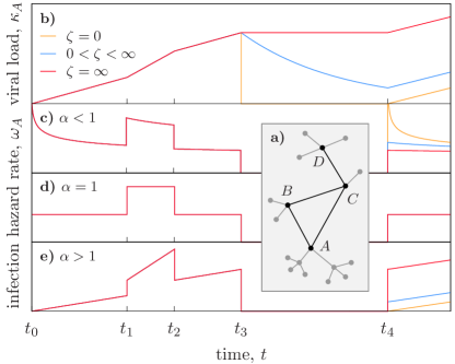
Figure 2: (a) Small system considered in example. (b) Evolution of node $A$’s viral load. In the interval ${t\in[t_{3},t_{4}]}$ node $A$ is dormant and its viral load decays instantly (orange), at a finite nonvanishing rate (blue), or accumulates perpetually (red). (c)-(e) Node $A$’s corresponding instantaneous infection rates, for (c) ${\alpha<1}$, (d) ${\alpha=1}$, and (e) ${\alpha>1}$, evaluated using Eq. (3). In the interval ${t\in[t_{3},t_{4}]}$ node $A$’s neighborhood is fully healthy and it cannot become infected (${\omega_{A}=0}$).

For illustrative purposes, consider the system depicted in Fig. 2(a), where all nodes are initially healthy except for $D$. Node $C$ becomes infected at time $t_{0}$ and subsequently infects $B$ at $t_{1}$. During the interval ${t\in[t_{0},t_{1}]}$, node $A$’s viral load, $\kappa_{A}$, grows with rate $\upsilon$, but from $t_{1}$ onwards it will increase with rate $2\upsilon$. At $t_{2}$, node $C$ recovers and $\kappa_{A}$ reduces its accumulation rate back to $\upsilon$, and when $B$ recovers at $t_{3}$, $\kappa_{A}$ starts to decay with relaxation time $\zeta$. Finally, $C$ becomes infected once again at $t_{4}$ and $\kappa_{A}$ resumes its growth at rate $\upsilon$. Figs. 2(b-e) show the evolution of $\kappa_{A}$ and $\omega_{A}$ for various $\zeta$ and $\alpha$. Hereafter we use temporal units such that $\eta=1$ and, without loss of generality, set ${\upsilon=1}$.

III Short-term memory

III.1 Analytics

We begin our analysis for ${\zeta=0}$, with dormant nodes instantly erasing their viral load. Thus, when the outbreak reenters their neighborhood, they become susceptible starting afresh (with ${\kappa=0}$). Hence, the only memory effect present is during the infection period, which we interpret as a short-term memory mode.

Each node is uniquely defined by its state, infected or healthy, and its accumulated viral load. The state of a node only changes with the transitions i) infected to healthy, and ii) susceptible to infected. When a node transitions between susceptible and dormant, its state remains unaltered. On the other hand, the viral load i) is erased instantly when an infected node recovers, ii) increases proportionally to the number of infected neighbors while a node is susceptible, and iii) is erased instantly when a susceptible node becomes dormant.

In the Supplemental Material (SM), we derive exact stochastic evolution equations for both the state and accumulated viral load of each node. Applying a mean-field approximation, these equations can be reduced to a single expression for the late-time prevalence, $\rho$, the average fraction of nodes that are infected in the steady-state (see SM for a detailed derivation). If all nodes have the same degree $k$, this equation reads

$$-\rho+ak\rho(1-\rho)-bk\rho(1-\rho)^{k}=0\ ,$$ (4)

with ${a>0}$. Roughly speaking, the first term corresponds to the recovery of infected nodes, the second term to the infection of susceptible nodes, and the third is related to susceptible nodes becoming dormant. The shape factor of the infection probability, $\alpha$, and the effective spreading ratio, $\lambda$, are encapsulated in $a$ and $b$, which become constant parameters when $\rho\approx 0$.

Equation (4) uncovers the existence of an epidemic threshold, where the population transitions from a healthy, pathogen-free state to an endemic, disease burdened one. Linear stability analysis reveals that the healthy phase, $\rho=0$, becomes unstable at ${a-b-1/k=0}$, yielding a phase transition at the critical point ${a_{\text{c}}=b+1/k}$. Moreover, the nature of the transition changes at ${a-bk=0}$, yielding a tricritical point at ${a_{\text{tc}}=1/(k-1)}$, ${b_{\text{tc}}=1/k(k-1)}$. Then the steady state is endemic for ${a>a_{\text{c}}}$, and the phase transition is continuous for ${b<b_{\text{tc}}}$ and discontinuous for ${b>b_{\text{tc}}}$. Finally, the prevalence of the endemic phase scales as ${\rho\propto(a-a_{\text{c}})^{\beta}}$, with ${\beta_{\text{c}}=1}$ when the transition is continuous, and ${\beta_{\text{tc}}=1/2}$ at the tricritical point.

Figure 3 shows the phase diagram in terms of the original parameters $\alpha$ and $\lambda$. We observe that the critical point initially increases monotonically with $\alpha$, but afterwards saturates for ${\alpha\rightarrow\infty}$. This result is consistent with the possibly largest epidemic threshold reported in Liu and Van Mieghem (2018). On the other hand, the transition to endemicity is discontinuous for ${\alpha>\alpha_{\text{tc}}\approx 2.348}$. Recall that the infection probability density presents a peak for ${\alpha>1}$, and, in fact, tends towards a delta function in the limit ${\alpha\rightarrow\infty}$. Thus, a node requires a quasi deterministic amount of viral load to become infected, mimicking a threshold model, which commonly exhibits a discontinuous phase transition Min and San Miguel (2018).

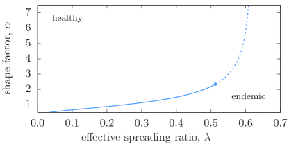
Figure 3: Phase diagram for ${\zeta=0}$. The solid lines indicates a continuous phase transition, the dashed line indicates a discontinuous phase transition, and the dot marks the tricritical point, ${\alpha_{\text{tc}}\approx 2.348}$, ${\lambda_{\text{tc}}\approx 0.513}$.

III.2 Simulations

In order to verify these analytic findings, we perform extensive stochastic simulations. We begin by exploring the position of the critical point, ${\lambda_{\text{c}}}$, that separates an absorbing (healthy) phase (${\lambda<\lambda_{\text{c}}}$) from an active (endemic) one (${\lambda>\lambda_{\text{c}}}$). The simulations start well into the active phase with a fully infected population, and quasistatically decrease the control parameter, $\lambda$, until finite-size fluctuations trap the system in the absorbing state. We sample the late-time prevalence, ${\rho_{\text{st}}=\lim_{t\rightarrow\infty}N_{\text{I}}(t)/N}$, of $10^{4}$ states, time-averaged over various trajectories (see SM for simulation details).

As shown in Fig. 4, ${\lambda_{\text{c}}}$ indeed increases with $\alpha$, and saturates for large values of $\alpha$. Moreover, for ${\alpha<1}$ the approach to the critical point is very similar to the standard SIS (${\alpha=1}$), consistent with a continuous phase transition with exponent ${\beta=1}$. On the other hand, for ${\alpha=4}$ the curves terminate at a remarkably high prevalence, consistent with a discontinuous phase transition. Finally, the curves for ${\alpha=2}$ also terminate at a rather high prevalence, which deviates from the analytic prediction. Nonetheless, since the apparent discontinuity decreases with the system size, this observation is most likely related to finite-size effects.

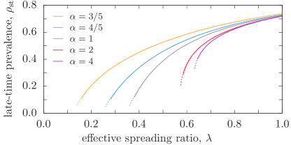
Figure 4: Late-time prevalence of the active steady state for networks of size ${N=10^{3}}$ (solid) and ${N=10^{4}}$ (dashed), with ${\zeta=0}$. Infection probability distributions with ${\alpha=3/5}$ (orange), ${\alpha=4/5}$ (blue), ${\alpha=1}$ (grey), ${\alpha=2}$ (red), and ${\alpha=4}$ (purple). Uncertainty bars not appreciable at this scale.

We complement these results with the analysis of patient zero scenarios, the arrival of an infected agent in a previously unaffected population. We employ the lifespan method Mata et al. (2015), which simulates outbreaks starting from a single infected node. Each single-seed realization is characterized by its coverage, $K$, defined as the number of distinct nodes that have become infected at least once, and can be either finite or endemic. While the former return to the absorbing state, the latter evolve towards an active steady state. In finite systems, we introduce a coverage threshold, ${K_{\text{th}}=c_{\text{th}}N}$, with ${0<c_{\text{th}}<1}$. A realization is declared endemic whenever its coverage reaches the threshold, and those that terminate without surpassing it are considered finite. As reported in Mata et al. (2015), the value of $c_{\text{th}}$ does not modify the qualitative results. Hereafter, we use ${c_{\text{th}}=0.75}$.

For a fixed value of $\lambda$ we run $10^{4}$ realizations, each starting with a single, randomly chosen infected node, and a system cleared of all viral load. If an outbreak becomes endemic, we extend the simulation until it reaches the steady-state, and then measure the late-time prevalence, $\rho_{\text{st}}^{*}$ (see SM for simulation details). The results are shown in Figs. 5(a,b), which include the previously computed ${\rho_{\text{st}}}$. While $\rho_{\text{st}}^{*}$ shows a discontinuous jump for $\alpha=4$, with $\alpha=2$ it grows continuously and coincides with $\rho_{\text{st}}$, supporting our analytical findings. Moreover, since ${\alpha=2}$ is close to tricritical point, a cross-over effect towards the exponent ${\beta_{\text{tc}}}$ is expected, explaining the rather steep approach towards the critical point.

Overall, these analytic and simulated results indicate that the system’s macroscopic properties are drastically affected by the microscopic details of the infection mechanism. In particular, the critical point that separates the healthy from the endemic phase grows with $\alpha$, and the nature of the phase transition changes from continuous to discontinuous at the tricrital point $\alpha_{\text{tc}}$.

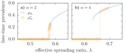
Figure 5: Late-time prevalence for quasistatic (blue curve) and single-seed (orange circles) simulations with ${\zeta=0}$ in a network of ${N=10^{4}}$ nodes, for (a) ${\alpha=2}$ and (b) ${\alpha=4}$. Uncertainty bars comparable to symbol size.

IV Long-term memory

Next, we consider the case ${\zeta=\infty}$, where a dormant node’s viral load remains frozen until the outbreak revisits its neighborhood. Besides the short-term memory present during the infection period, nodes now possess an additional long-term memory mode that is capable of connecting very distant temporal points, causing the system to evolve in a highly nonlinear manner.

As before, the state of a node changes with the transitions i) infected to healthy, and ii) susceptible to infected. On the other hand, the viral load i) is instantly erased when an infected node recovers, ii) increases proportionally to the number of infected neighbors while a node is susceptible, and iii) remains constant while the node is dormant. We can write an equation for the state of node $i$ (${n_{i}=1}$ if its infected, ${n_{i}=0}$ if its healthy), and obtain the expected value in the steady-state (see SM for a detailed derivation). The resulting equation reads

$$\langle n_{i}\rangle=\lambda\langle(1-n_{i})z_{i}\rangle\ ,$$ (5)

with ${z_{i}=\sum_{j}a_{ij}n_{j}}$ the number of infected neighbors, and $a_{ij}$ the elements of the adjacency matrix. Note that this equation is derived without implementing a mean-field approximation.

Surprisingly, Eq. (5) is identical to the first-order equation of the standard SIS model Pastor-Satorras et al. (2015) and, therefore, both the miccSIS and SIS models have the same mean field description. Thus, whenever the standard SIS dynamics is well described by its mean field approximation, as is the case for random degree-regular networks, the miccSIS dynamics is also aptly described by the same mean field equation. This equivalence demonstrates that the late-time prevalence is independent of $\alpha$, and identical to the Markovian model. This result is verified by stochastic simulations, shown in Fig. 6. Indeed we observe that the late-time prevalence curves coincide for all values of $\alpha$. A small deviation occurs in the critical region (see inset of Fig. 6), which is caused by finite size fluctuations.

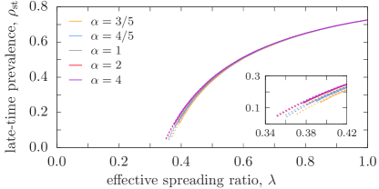
Figure 6: Late-time prevalence of the active steady state for networks of size ${N=10^{3}}$ (solid) and ${N=10^{4}}$ (dashed), with ${\zeta=\infty}$. Infection probability distributions with ${\alpha=3/5}$ (orange), ${\alpha=4/5}$ (blue), ${\alpha=1}$ (grey), ${\alpha=2}$ (red), and ${\alpha=4}$ (purple). Uncertainty bars not appreciable at this scale.

Compared to the short-term memory mode, for ${\alpha>1}$ (respectively, ${\alpha<1}$) the endemic phase is enlarged (shrunken) by the long-term mode. This phenomenon is explained by the monotonically increasing (decreasing) infection rate. When the outbreak revisits a dormant node’s neighborhood, its previously accumulated viral load facilitates (hinders) reinfection, enabling (preventing) the outbreak to remain active in a wider range of $\lambda$. These results reveal that the additional long-term memory completely suppresses the effects of the short-term mode. Specifically, it causes individuals with virtually infinite memory to behave, on the aggregate, as if they had no memory at all. This collective memory loss consequently renders the system’s macroscopic state unable to distinguish between agents’ microscopic properties.

In order to elucidate these findings, we proceed with the analysis of patient zero scenarios, where an infected agent arrives in a previously unaffected population. For a fixed value of $\lambda$ we run $10^{4}$ realizations, each starting with a single, randomly chosen infected node, and a system cleared of all viral load. We measure the average coverage fraction, ${\bar{c}=\langle K\rangle/N}$, and the probability that a realization surpasses the coverage threshold, $P_{1}$, which serves as a proxy for the true endemic probability, $P_{\infty}$, the probability, in the thermodynamic limit, that an outbreak becomes endemic (see SM for simulation details).

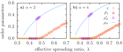
Figure 7: Average coverage (orange circles), endemic probability (red diamonds), and late-time prevalences (purple squares and blue curve) with ${\zeta=\infty}$ in a network of ${N=10^{4}}$ nodes, for (a) ${\alpha=2}$ and (b) ${\alpha=4}$. Uncertainty bars not appreciable at this scale.

IV.1 Bistability

We first analyze $\alpha>1$, for which the infection probability presents a peak and the instantaneous infection rate increases monotonically with the accumulated viral load. The patient zero results are shown in Figs. 7(a,b), which include the previously computed ${\rho_{\text{st}}}$, and the late-time prevalence of single-seed outbreaks that are able to become endemic, ${\rho_{\text{st}}^{*}}$ (see SM for simulation details). We find that the average coverage, $\bar{c}$, and the endemic probability, $P_{1}$, coincide for all values of $\lambda$ and present a continuous phase transition at ${\lambda_{\text{c}}(\bar{c})}$. However, this point is notably larger than the critical point of the late-time prevalence, ${\lambda_{\text{c}}(\rho_{\text{st}})}$. While $\rho_{\text{st}}$ presents a continuous phase transition, $\rho_{\text{st}}^{*}$ exhibits a discontinuous phase transition at ${\lambda_{\text{c}}(\rho_{\text{st}}^{*})=\lambda_{\text{c}}(\bar{c})}$. As expected, the two prevalence curves overlap after the abrupt jump.

This evidences the existence of an intermediate region ${\lambda\in[\lambda_{\text{c}}(\rho_{\text{st}}),\lambda_{\text{c}}(\bar{c})]}$ where all single-seed outbreaks return to the absorbing state, whereas fully infected populations evolve towards an active steady state. The key ingredient to understand this phenomenon is the environment of frozen viral load. During the simulations that measure the late-time prevalence, the viral loads are well thermalized, enabling the outbreak to remain in an active state. Conversely, this environment is deficient in single-seed outbreaks, as the system has not yet reached its steady state. Hence, outbreaks are unable to produce sufficient new infections and rapidly become trapped in the absorbing state.

These results indicate that the system displays two attractors in this intermediate region. Then, for ${\zeta=\infty}$ and ${\alpha>1}$ the system’s phase diagram exhibits an additional bistable phase, that separates the usual healthy and endemic phases. The associated hysteresis loop, however, has a rather exotic nature: although its lower branch presents the expected discontinuity, the upper branch connects the two attractors in a continuous manner. This contrasts with previous findings of bistability, were the hysteresis loop is bounded by two discontinuities Dodds and Watts (2004); Gómez-Gardeñes et al. (2016); Chen et al. (2018). Moreover, the transition to full endemicity is hybrid Cai et al. (2015): the endemic probability grows continuously at $\lambda_{\text{c}}(\rho_{\text{st}}^{*})$, but the late-time prevalence jumps discontinuously.

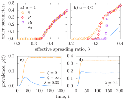
Figure 8: (Top) Average coverage (orange circles), endemic probabilities (red diamonds and purple squares), and late-time prevalence (blue curve) with ${\zeta=\infty}$ in a network of ${N=10^{4}}$ nodes, for (a) ${\alpha=1}$ and (b) ${\alpha=4/5}$. Uncertainty bars not appreciable at this scale. (Bottom) Evolution of single-seed outbreaks that reach the coverage threshold once for ${\alpha=4/5}$, with $\zeta=0$ (orange) and ${\zeta=\infty}$ (blue) in a network of ${N=10^{4}}$ nodes, for (c) ${\lambda=0.33}$ and (d) ${\lambda=0.4}$, averaged over $10^{2}$ trajectories. Uncertainty bars not appreciable at this scale.

IV.2 Excitability

Finally, we study $\alpha<1$, for which the infection probability presents power-law-like fat tails an the instantaneous infection rate decreases monotonically with the accumulated viral load. In Figs. 8(a,b) we show the patient zero analysis for the standard SIS (${\alpha=1}$) and broad-tailed infection distributions (${\alpha<1}$). Here, we additionally compute $P_{3}$, the probability that a single-seed outbreak reaches the coverage threshold three times (see SM for simulation details). With $\alpha=1$, $P_{1}$ and $P_{3}$ are practically identical, indicating that an outbreak that surpasses the coverage threshold once remains active long enough to surpass the threshold two more times. Thus $P_{1}$ is an adequate proxy for the true endemic probability, $P_{\infty}$, which additionally coincides with $\bar{c}$ and $\rho_{\text{st}}$.

For ${\alpha<1}$ the situation is quite different. Firstly, the average coverage starts growing continuously at ${\lambda_{\text{c}}(\bar{c})}$, when all other order parameters are still identically zero. Additionally, the transition point of $P_{1}$ is significantly lower than that of $P_{3}$. Thus, there is a wide interval where all outbreaks that surpass the threshold once eventually terminate in the absorbing state, evidencing the inadequateness of $P_{1}$ as a measure of the true endemic probability. The inflection point of $P_{3}$ is much closer to the transition point of ${\rho_{\text{st}}}$, which suggests that the critical point of the endemic probability ($P_{\infty}$, the probability to surpass the threshold an infinite amount of times) coincides with ${\lambda_{\text{c}}(\rho_{\text{st}})}$. Beyond this point, $P_{\infty}$ is expected to coincide with $\bar{c}$, indicating that the endemic probability presents a discontinuous phase transition. Then, the transition to full endemicity is again hybrid. Nonetheless, here the late-time prevalence grows continuously, while the endemic probability jumps discontinuously.

In this case, we find an intermediate region ${\lambda\in[\lambda_{\text{c}}(\bar{c}),\lambda_{\text{c}}(\rho_{\text{st}})]}$ where outbreaks are unable to become endemic (${P_{\infty}=0}$) but affect a macroscopic fraction of the population (${c>0}$). In Figs. 8(c,d) we show the prevalence, ${\bar{\rho}(t)=\langle N_{\text{I}}(t)\rangle/N}$, of realizations that surpass the coverage threshold once, for ${\lambda=0.33}$ and ${\lambda=0.4}$. We include the results for ${\zeta=0}$ for comparison (see SM for simulation details). Both values of $\lambda$ are located in the active phase of the short-term memory mode (${\zeta=0}$), and so the endemic realizations converge monotonically towards their active steady states. For the long-term memory mode (${\zeta=\infty}$), ${\lambda=0.33}$ is located in the intermediate region. In this case, we observe that outbreaks grow up to a maximum, after which their prevalence gradually diminishes until they reach the absorbing state. This behavior is typically observed in SIR-like dynamics and is reminiscent of excitable media. In the endemic phase (${\lambda=0.4}$) the outbreaks continue presenting a peak, but afterwards relax towards an active steady state.

In conclusion, for ${\zeta=\infty}$ and ${\alpha<1}$ the usual healthy and endemic phases are separated by an additional excitable phase. This excitable behavior is again a consequence of the environment of frozen viral load. Independently of $\zeta$, an outbreak starts from a single infected node in a population cleared of viral load. Then it initially evolves as if the agents only had the short-term memory mode (clearly appreciable for $t\in[0,25]$ in Fig. 8(c)), rapidly achieving a large coverage. When the outbreak revisits a previously affected area, the long-term memory mode is activated and the frozen viral load impedes new infections. Thus, dormant nodes are effectively removed from the dynamic, impede the outbreak to grow, and eventually cause its extinction. To the extend of our knowledge, this excitable behavior has not been previously reported in comparable SIS-like models.

V Conclusions

All these results show a crucial feature of agents that possess the long-term memory mode. Focusing only on the late-time prevalence of fully infected populations provides little insight about the system’s constituents. Nevertheless, widely distinct and clearly distinctive behaviors appear with the analysis of patient zero scenarios. Moreover, a common effect of agents’ memory is the breaking of the symmetry between the order parameters $\bar{c}$, $P$, and ${\rho_{\text{st}}}$. If agents are memoryless, all three order parameters are completely identical. This symmetry is broken when agents possess a long-term memory mode, and the critical points become dissociated. The system first transitions from the healthy phase to an either bistable or excitable intermediate regime, followed by a hybrid transition to the endemic phase. This differs from a double phase transition, where the same order parameter undergoes two consecutive phase transitions, a phenomenon usually associated to node and/or topological heterogeneities Dodds and Watts (2004); Chen et al. (2018); Colomer-de-Simón and Boguñá (2014); Allard et al. (2017).

The analysis of our stylized, yet feature-rich model evidences a crucial role of non-Markovianity in the spread of epidemic outbreaks. In particular, the agents’ memory range dramatically impacts the outbreak of newly introduced pathogens. This topic is currently a very active field of epidemic modeling, with applications ranging from the appearance of exotic diseases, to the dissemination of fake news on social media.

Nonetheless, further research is necessary. A thorough study of finite, non-vanishing relaxation times of the viral load of dormant nodes can aid in further elucidating the interplay between memory modes, and its effects on the system’s properties. Furthermore, the inclusion of nontrivial contact networks will supply renewed insight on the relevance of microscopic mechanisms and topological properties in dynamical processes on networks.

Appendix A Non-Markovian Gillespie algorithm

A.1 General framework

Here, we summarize the derivation reported in Boguñá et al. (2014). Consider a set of $M$ statistically independent, discrete, stochastic processes, each with an interevent time distribution ${\psi_{j}(t)}$ and corresponding survival probability ${\Psi_{j}(t)=\int_{t}^{\infty}\psi_{j}(t^{\prime})\text{d}t^{\prime}}$. At a certain moment in time $t_{0}$, process $j$ has been active for $t_{j}$ units of time. Let ${\phi(\tau,i|\{t_{k}\})\text{d}\tau}$ denote the joint probability that the next-occurring event takes place in the interval ${t\in[t_{0}+\tau,t_{0}+\tau+\text{d}\tau]}$ and corresponds to process $i$, conditioned by the set of elapsed times $\{t_{k}\}$. This probability density can be expressed as

$$\phi(\tau,i|\{t_{k}\})=\frac{\psi_{i}(t_{i}+\tau)}{\Psi_{i}(t_{i}+\tau)}\Phi(\tau|\{t_{k}\})\ ,$$ (6)

where

$$\Phi(\tau|\{t_{k}\})=\prod_{j=1}^{M}\frac{\Psi_{j}(t_{j}+\tau)}{\Psi_{j}(t_{j})}$$ (7)

is the survival probability of $\tau$, i.e., the conditional probability that no event takes place before ${t_{0}+\tau}$. Then the probability that the next event takes place in the interval ${t\in[t_{0},t_{0}+\tau]}$ is

$$\Xi(\tau|\{t_{k}\})=1-\Phi(\tau|\{t_{k}\})\ .$$ (8)

Once the interval $\tau$ is known, the probability that the next-occurring event corresponds to process $i$ is given by

$$\Pi(i|\tau,\{t_{k}\})=\frac{\omega_{i}(t_{i}+\tau)}{\sum_{j=1}^{M}\omega_{j}(t_{j}+\tau)}\ ,$$ (9)

with ${\omega_{j}(t)=\psi_{j}(t)/\Psi_{j}(t)}$ the instantaneous hazard rate of process $j$.

Eqs. (8) and (9) provide an algorithm that generates statistically correct sequences of events: i) draw the interval by solving ${\Xi(\tau|\{t_{k}\})=u}$, with ${u\in U(0,1)}$, ii) increase the system time as ${t\leftarrow t+\tau}$, iii) draw the process from the discrete distribution ${\Pi(i|\tau,\{t_{k}\})}$, iv) revise the list of active processes, and v) update the set of elapsed times as ${t_{j}\leftarrow t_{j}+\tau}$ (setting ${t_{j}=0}$ for newly activated processes).

A.2 Incorporating viral loads

Recoveries are straightforwardly incorporated into this framework, with the elapsed time $t_{j}$ measuring the period since agent $j$ became infected (i.e., this occurred at ${t=t_{0}-t_{j}}$). On the other hand, infection processes require the translation of infection probability densities into interevent time distributions. Consider susceptible agent $j$, characterized by its infection probability density ${\psi^{*}_{j}(\kappa)}$ and corresponding survival probability ${\Psi_{j}^{*}(\kappa)=\int_{\kappa}^{\infty}\psi^{*}_{j}(\kappa^{\prime})\text{d}\kappa^{\prime}}$. Its interevent time distribution, ${\psi_{j}(t)}$, is given by the normalization condition

$$\psi_{j}(t)\text{d}t=\psi_{j}^{*}(\kappa)\text{d}\kappa\ .$$ (10)

Since the activity in $j$’s neighborhood may vary over time, the rate at which it amasses viral load is generally nonconstant. At time $t$ it has amassed ${\kappa_{j}(t)}$ units of viral load and has ${z_{j}(t)}$ infected neighbors. If the system remains unaltered in an interval ${\text{d}t}$, node $j$ will amass an additional ${\text{d}\kappa=\tilde{\upsilon}_{j}\text{d}t}$, with ${\tilde{\upsilon}_{j}(t)=\sum_{i=1}^{z_{j}(t)}\upsilon_{i}}$ its instantaneous amassment rate. Substituting in Eq. (10) we find

$$\psi_{j}(t)=\tilde{\upsilon}_{j}(t)\psi_{j}^{*}(\kappa_{j}(t))\ .$$ (11)

For the survival probability we have

$$\Psi_{j}(t)=\int_{t}^{\infty}\psi_{j}(t^{\prime})\text{d}t^{\prime}=\int_{\kappa_{j}(t)}^{\infty}\psi^{*}_{j}(\kappa^{\prime})\text{d}\kappa^{\prime}=\Psi^{*}_{j}(\kappa_{j}(t))\ ,$$ (12)

which yields its instantaneous hazard rate

$$\omega_{j}(t)=\tilde{\upsilon}_{j}(t)\frac{\psi_{j}^{*}(\kappa_{j}(t))}{\Psi_{j}^{*}(\kappa_{j}(t))}\ .$$ (13)

Note that we can always write ${t=t_{0}+\tau}$, with $t_{0}$ the time at which the system was last updated, and ${\tau\geq 0}$. Then, the instantaneous amassment rate remains constant in the interval ${[t_{0},t]}$, ${\tilde{\upsilon}_{j}(t)=\tilde{\upsilon}_{j}(t_{0})}$, and ${\kappa_{j}(t)=\kappa_{j}(t_{0})+\tau\tilde{\upsilon}_{j}(t_{0})}$.

In our work, infections are governed by a Weibull distribution with shape parameter $\alpha$ and scale parameter $\mu$,

$$\psi_{\text{inf}}^{*}(\kappa)=\alpha\mu^{\alpha}\kappa^{\alpha-1}e^{-(\mu\kappa)^{\alpha}}\hskip 24.0pt\Psi_{\text{inf}}^{*}(\kappa)=e^{-(\mu\kappa)^{\alpha}}\ ,$$ (14)

and recoveries by a Poisson process with rate $\eta$,

$$\psi_{\text{rec}}(t)=\eta e^{-\eta t}\hskip 24.0pt\Psi_{\text{rec}}(t)=e^{-\eta t}\ .$$ (15)

Since all infectors have the same infectivity rate $\upsilon$, the instantaneous amassment rate of a susceptible node $j$ becomes ${\tilde{\upsilon}_{j}(t)=\upsilon z_{j}(t)}$, with $z_{j}(t)$ the number of its neighbors that are infected at time $t$. So the instantaneous hazard rates for infections and recoveries are, respectively, ${\omega_{\text{inf}}(t)=\upsilon\alpha\mu^{\alpha}z(t)[\kappa(t)]^{\alpha-1}}$ and ${\omega_{\text{rec}}(t)=\eta}$.

Appendix B Simple and complex contagion

B.1 Simple contagion

Simple contagion describes purely dyadic interactions, thus we can identify each edge that connects a healthy node with an infected one as an isolated transmission channel. Consider at time $t$ a susceptible node $j$ and its infected neighbor $i$, which became infected at ${t_{i}<t}$. The probability that node $i$ infects node $j$ within the interval $(t,t+\text{d}t)$ is ${\omega_{i\rightarrow j}(t|t_{i})\text{d}t}$, regardless of the rest of the system. If node $j$ has ${z_{j}(t)}$ infectors at time $t$, the previous statement holds for each of them.

The total probability that node $j$ becomes infected at time $t$ depends on all of its incoming transmission channels. Since these are statistically independent, we can write

$$\omega_{j}(t)=\sum_{i=1}^{z_{j}(t)}\omega_{i\rightarrow j}(t|t_{i})\ ,$$ (16)

where $\omega_{j}(t)$ is the instantaneous hazard rate of node $j$’s infection process (i.e., the probability per unit of time that node $j$ becomes infected at time $t$). Using

$$\Omega_{j}(t)=\frac{1}{z_{j}(t)}\sum_{i=1}^{z_{j}(t)}\omega_{i\rightarrow j}(t|t_{i})$$ (17)

we can write Eq. (16) as

$${\omega_{j}(t)=\Omega_{j}(t)z_{j}(t)}\ ,$$ (18)

thus the total hazard rate is proportional to the number of current infectors. If ${\omega_{i\rightarrow j}(t|t_{i})=\beta}$ are constants (and homogenous for all pairs of nodes), we recover the standard SIS model with the familiar expression ${\omega_{j}(t)=\beta z_{j}(t)}$. When the transmission rates ${\omega_{i\rightarrow j}}$ are time-dependent, the dynamics has memory effects; thus, simple contagion can be non-Markovian (as in Starnini et al. (2017), for example).

B.2 Complex contagion

When the dynamics are described by interactions that are not strictly dyadic, the contagion becomes complex. These processes usually incorporate an explicit social reinforcement or inhibition mechanism. Although the classification of complex contagion processes is yet to be formalized, they can be broadly categorized into two groups:

• In edge-centric approaches, one still considers the transmission channel from infected node $i$ to susceptible node $j$. Now, however, the transmission rate ${\omega_{i\rightarrow j}}$ is affected by the neighborhoods of $i$ and/or $j$ (for specific examples, see Pérez-Reche et al. (2011); Gómez-Gardeñes et al. (2016); Liu et al. (2017)). Considering only nearest-neighbors, the transmission rate from node $i$ to node $j$ at time $t$, ${\omega_{i\rightarrow j}(t|z_{i}(t),z_{j}(t))}$, is a function of their current infected neighbors, $z_{i}(t)$ and $z_{j}(t)$. Although we can still write the total hazard rate ${\omega_{j}(t)}$ as in Eq. (16), the instantaneous average defined in Eq. (17) has an explicit dependence on $z_{i}(t)$ and $z_{j}(t)$. Consequently, ${\omega_{j}(t)}$ can be superlinear (reinforcement) or sublinear (inhibition) with the number of current infectors, ${z_{j}(t)}$.

• On the other hand, node-centric approaches forgo the notion of transmission channels and directly prescribe the instantaneous hazard rate, ${\omega_{j}(t)}$. These usually incorporate thresholds, such as ${\omega_{j}(t)=\delta(T_{j}-z_{j}(t))}$ Watts (2002) or ${\omega_{j}(t)=z_{j}(t)\Theta(T_{j}-z_{j}(t))+\beta\Theta(z_{j}(t)-T_{j})}$ O’Sullivan et al. (2015), which explicitly evidence the nonlinearity of ${\omega_{j}(t)}$ with ${z_{j}(t)}$.

B.3 Memory-induced complex contagion

Consider an isolated pair of nodes $i$ and $j$ in the miccSIS model. Both are healthy when node $i$ becomes infected at time $t_{i}$. The total amount of viral load that $j$ has amassed at time $t>t_{i}$ is $\kappa_{j}(t)=\upsilon(t-t_{i})$. The instantaneous hazard rate of node $j$’s infection is

$$\omega_{j}(t)=\upsilon\alpha\mu^{\alpha}z_{j}(t)[\kappa_{j}(t)]^{\alpha-1}\ ,$$ (19)

but since $j$ has only one infected neighbor, it is given solely by the exposure to node $i$: $\omega_{j}(t)=\omega_{i\rightarrow j}(t|t_{i})$, with

$$\omega_{i\rightarrow j}(t|t_{i})=\upsilon\alpha\mu^{\alpha}[\upsilon(t-t_{i})]^{\alpha-1}\ .$$ (20)

Now consider an infected node $j$ that at time $t_{0}$ recovers and becomes dormant (all its neighbors are healthy). At time $t$ it has a set of $\{i\}$ infected neighbors that became infected at times $\{t_{i}\}$, with ${t_{0}<t_{i}<t}$, ${\forall i=1,2,...,z_{j}(t)}$. The total amount of viral load that $j$ has amassed at time $t$ is

$$\kappa_{j}(t)=\chi(t)+\sum_{i=1}^{z_{j}(t)}\upsilon(t-t_{i})\ ,$$ (21)

where $\chi(t)$ stores the viral load accumulated from neighbors that became infected in the interval ${(t_{0},t)}$ but are currently healthy. Substituing Eq. (21) in Eq. (19), we find

$$\omega_{j}(t)=\upsilon\alpha\mu^{\alpha}z_{j}(t)\left[\chi(t)+\sum_{i=1}^{z_{j}(t)}\upsilon(t-t_{i})\right]^{\alpha-1}\ ,$$ (22)

which, using Eq. (20), can be written for $\alpha\neq 1$ as

$$\omega_{j}(t)=z_{j}(t)\left[(\upsilon\alpha\mu^{\alpha})^{\frac{1}{\alpha-1}}\chi(t)+\sum_{i=1}^{z_{j}(t)}\left[\omega_{i\rightarrow j}(t|t_{i})\right]^{\frac{1}{\alpha-1}}\right]^{\alpha-1}\ .$$ (23)

Notice that Eq. (23) cannot be written as Eq. (16). Therefore, while the exposures to infectious sources are initially described as isolated events, the agents’ memory causes them to become entangled. For instance, for $\alpha=2$, Eq. (23) can be written as

$$\omega_{j}(t)=2\upsilon\mu\chi(t)z_{j}(t)+\Omega(t)[z_{j}(t)]^{2}$$ (24)

which has an explicit quadratic dependence on $z_{j}(t)$ . The simple contagion of the standard SIS model can be recovered only with $\alpha=1$, for which Eq (19) equates with Eq (18). In conclusion, the non-Markovianity of the miccSIS model induces an effective social reinforcement/inhibition even though it was not incorporated in the initial description of the model.

References

- Anderson and May (1991) R. M. Anderson and R. M. May, Infectious Diseases of Humans (Oxford University Press, Oxford, 1991).
- Pastor-Satorras and Vespignani (2001) R. Pastor-Satorras and A. Vespignani, Phys. Rev. Lett. 86, 3200 (2001).
- Bond et al. (2012) R. M. Bond, C. J. Fariss, J. J. Jones, A. D. I. Kramer, C. Marlow, J. E. Settle, and J. H. Fowler, Nature 489, 295 (2012).
- Colizza et al. (2007) V. Colizza, A. Barrat, M. Barthelemy, A.-J. Valleron, and A. Vespignani, PLOS Med. 4, e13 (2007).
- Vespignani (2012) A. Vespignani, Nat. Phys. 8, 32 (2012).
- Pastor-Satorras et al. (2015) R. Pastor-Satorras, C. Castellano, P. Van Mieghem, and A. Vespignani, Rev. Mod. Phys. 87, 925 (2015).
- Colizza et al. (2006) V. Colizza, A. Barrat, M. Barthelemy, and A. Vespignani, Proc. Natl. Acad. Sci. U.S.A. 103, 2015 (2006).
- Balcan et al. (2009) D. Balcan, V. Colizza, B. Gonçalves, H. Hu, J. J. Ramasco, and A. Vespignani, Proc. Natl. Acad. Sci. U.S.A. 106, 21484 (2009).
- Tizzoni et al. (2012) M. Tizzoni, P. Bajardi, C. Poletto, J. J. Ramasco, D. Balcan, B. Gonçalves, N. Perra, V. Colizza, and A. Vespignani, BMC Med. 10, 165 (2012).
- Streftaris and Gibson (2012) G. Streftaris and G. J. Gibson, Biostatistics 13, 580 (2012).
- Chowell and Nishiura (2014) G. Chowell and H. Nishiura, BMC Med. 12, 196 (2014).
- Oliveira and Barabasi (2005) J. G. Oliveira and A.-L. Barabasi, Nature 437, 1251 (2005).
- González et al. (2008) M. C. González, C. A. Hidalgo, and A.-L. Barabási, Nature 453, 779 (2008).
- Ben-Jacob et al. (1994) E. Ben-Jacob, O. Schochet, A. Tenenbaum, I. Cohen, A. Czirók, and T. Vicsek, Nature 368, 46 (1994).
- Donabedian (2003) H. Donabedian, J. Infect. 46, 207 (2003).
- Castellano et al. (2009) C. Castellano, S. Fortunato, and V. Loreto, Rev. Mod. Phys. 81, 591 (2009).
- Centola (2010) D. Centola, Science 329, 1194 (2010).
- Hodas and Lerman (2014) N. O. Hodas and K. Lerman, Sci. Rep. 4, 4343 (2014).
- Choi et al. (2017a) W. Choi, D. Lee, and B. Kahng, Phys. Rev. E 95, 022304 (2017a).
- Choi et al. (2017b) W. Choi, D. Lee, and B. Kahng, Phys. Rev. E 95, 062115 (2017b).
- Van Mieghem and van de Bovenkamp (2013) P. Van Mieghem and R. van de Bovenkamp, Phys. Rev. Lett. 110, 108701 (2013).
- Kiss et al. (2015) I. Z. Kiss, G. Röst, and Z. Vizi, Phys. Rev. Lett. 115, 078701 (2015).
- Starnini et al. (2017) M. Starnini, J. P. Gleeson, and M. Boguñá, Phys. Rev. Lett. 118, 128301 (2017).
- Dodds and Watts (2004) P. S. Dodds and D. J. Watts, Phys. Rev. Lett. 92, 218701 (2004).
- Lü et al. (2011) L. Lü, D.-B. Chen, and T. Zhou, New J. Phys. 13, 123005 (2011).
- Liu et al. (1987) W. Liu, H. W. Hethcote, and S. A. Levin, J. Math. Biol. 25, 359 (1987).
- Boguñá et al. (2014) M. Boguñá, L. F. Lafuerza, R. Toral, and M. Á. Serrano, Phys. Rev. E 90, 042108 (2014).
- Pérez-Reche et al. (2011) F. J. Pérez-Reche, J. J. Ludlam, S. N. Taraskin, and C. A. Gilligan, Phys. Rev. Lett. 106, 218701 (2011).
- Gómez-Gardeñes et al. (2016) J. Gómez-Gardeñes, L. Lotero, S. N. Taraskin, and F. J. Pérez-Reche, Sci. Rep. 6, 19767 (2016).
- Watts (2002) D. J. Watts, Proc. Natl. Acad. Sci. U.S.A. 99, 5766 (2002).
- Centola et al. (2007) D. Centola, V. M. Eguíluz, and M. W. Macy, Physica A 374, 449 (2007).
- Granell et al. (2013) C. Granell, S. Gómez, and A. Arenas, Phys. Rev. Lett. 111, 128701 (2013).
- Fu et al. (2017) F. Fu, N. A. Christakis, and J. H. Fowler, Sci. Rep. 7, 43634 (2017).
- Christakis and Fowler (2007) N. A. Christakis and J. H. Fowler, N. Engl. J. Med. 357, 370 (2007).
- Christakis and Fowler (2008) N. A. Christakis and J. H. Fowler, N. Engl. J. Med. 358, 2249 (2008).
- Cox (1970) D. Cox, Renewal theory (Methuen & Co., London, 1970).
- Liu and Van Mieghem (2018) Q. Liu and P. Van Mieghem, Phys. Rev. E 97, 022309 (2018).
- Min and San Miguel (2018) B. Min and M. San Miguel, Scientific Reports 8, 10422 (2018).
- Mata et al. (2015) A. S. Mata, M. Boguñá, C. Castellano, and R. Pastor-Satorras, Phys. Rev. E 91, 052117 (2015).
- Chen et al. (2018) X. Chen, R. Wang, M. Tang, S. Cai, H. E. Stanley, and L. A. Braunstein, New J. Phys. 20, 013007 (2018).
- Cai et al. (2015) W. Cai, L. Chen, F. Ghanbarnejad, and P. Grassberger, Nat. Phys. 11, 936 (2015).
- Colomer-de-Simón and Boguñá (2014) P. Colomer-de-Simón and M. Boguñá, Phys. Rev. X 4, 041020 (2014).
- Allard et al. (2017) A. Allard, B. M. Althouse, S. V. Scarpino, and L. Hébert-Dufresne, Proc. Natl. Acad. Sci. U.S.A. 114, 8969 (2017).
- Liu et al. (2017) Q.-H. Liu, W. Wang, M. Tang, T. Zhou, and Y.-C. Lai, Phys. Rev. E 95, 042320 (2017).
- O’Sullivan et al. (2015) D. J. O’Sullivan, G. O’Keeffe, P. Fennell, and J. Gleeson, Front. Phys. 3, 71 (2015).
- Note (1) Notice, however, that the terms and are stochastic processes that play an important role in the global dynamics.