Slow-roll Analysis of Double Field Axion Inflation^∗

MAN Ping Kwan, Ellgan^a)†

We adopt the double field natural inflation model motivated by the non-perturbative effects of supergravity and superstring theory to do the slow roll analysis. We show that when the parameters are suitably chosen, there exist ranges of initial values of fields that can satisfy the constraints of Planck observations. This implies less fine tuning of field values can be allowed with tolerance of $4{M}_{\text{pl}}$ for ${\phi}_{1}$ and $5{M}_{\text{pl}}$ for ${\phi}_{2}$ respectively, which become more physical for field fluctuation in quantum era. We also show that the spectral index ${n}_{\mathcal{RR}}$, the fraction of entropic power spectrum and the fraction of power spectra (so-called ${\beta}_{\text{iso}}$) and $\cos{\Delta}$ can satisfy the constraints of Planck observation. This implies that double field natural inflation is a valid model to describe cosmological inflation.

Keywords:

Superstring Theory, Double Field Inflation, Natural Inflation

1 Introduction

1.1 Present Observations for Inflation

So far, there have been many theoretical approaches to study inflation dynamics, with the verification via Planck data. It has been shown that in single field inflation models, Starobinsky model, power law model, D-brane model and hilltop quartic model match with the Planck data between $50$ and $60$ e-folds [3], while the constraints of slow-roll parameters, spectral index and its runnings are given in Table 1.

Multiple scalar fields are usually included in inflation models under the motivation of high energy physics [4] [5]. Unlike single field models, in which only adiabatic perturbation is present, multifield models generically produce entropic perturbation apart from adiabatic counterpart. The entropic perturbation can contribute to the adiabatic perturbation, thereby supporting inflation dynamics. [20] [6]. Hence, understanding the evolution of entropic perturbation and its coupling with adiabatic one are vital for studying non-trivial features of inflation that are not present in the single field cases.

Even though single field natural inflation can be derived from superstring theory [14], recent investigation shows that it is disfavoured by Planck 2018 observation [3]. The reasons are because it has a low Bayes factor of $\ln{B}=-4.2$ and its prediction of the tensor-to-scalar ratio against spectral index cannot enter the innermost region of Planck 2018 observation [3].

Slow-roll parameters	Range(s)	Spectral indices	Range(s)
${\epsilon}_{V}$	$<0.0053$	${n}_{s}-1$	$[-0.0423,-0.0327]$
${\eta}_{V}$	$[-0.021,-0.008]$	${\alpha}_{s}:=\frac{d{n}_{s}}{d\ln{k}}$	$[-0.008,0.012]$
${\xi}_{V}$	$[-0.0045,0.0096]$	${\beta}_{s}:=\frac{d^{2}{n}_{s}}{d\ln{k}^{2}}$	$[-0.003,0.023]$
		$\ln(10^{10}A_{s})$	$[3.03,3.058]$

Table 1: Slow roll potential parameters and spectral indices in Planck 2018

1.2 Main theme of this paper

Despite this, nowadays, superstring theory is the most promising theory for quantum gravity. Some considered the possibility of multi-field inflation [9]. In particular, some investigated the possibility of double inflation dynamics [12]. Thus, we raise questions, ”What will be the dynamics if double field natural inflation is considered? Can it satisfy the recent Planck observational constraints?” In this paper, we show that when the parameters are suitably chosen, there exist ranges of initial values of fields that can satisfy the constraints of Planck observations. Particularly, the predictions of spectral index ${n}_{\mathcal{RR}}$, tensor-to-scalar ratio $r$, ${\beta}_{\text{iso}}$ and $\cos{\Delta}$ are within the ranges of the present observation. This means that some specially chosen parameters can allow less fine tuning of field values, which become more physical for field fluctuation in quantum era.

The arrangement of this paper is as follows. In section 2, starting from a short review of single field natural inflation, we show how the double field natural inflation can be obtained by field stabilisation, whose ideas is to set those fields irresponsible for the inflation as a certain value such that the resulting inflation potential can be minimum along that field direction. In section 3, following the arguments in [6] and [7], we introduce the concepts of entropic perturbation, and derive the corresponding spectral index ${n}_{\mathcal{RR}}$, tensor-to-scalar ratio $r$, ${\beta}_{\text{iso}}$ and $\cos{\Delta}$. In section 4, we show how less fine tuning can be achieved by some choices of parameters, and evaluate all the related inflation parameters accordingly. Finally, in section 5, we explain the data.

2 Mathematical Derivation

2.1 A short review of single field natural inflation

Axions are hypothetical particles associated with the spontaneously broken Peccei-Quinn (PQ) symmetry that can solve the strong CP problem in QCD [21] [22]. After that, physicists adopted the idea of axion in superstring theory that they realize aligned natural inflation on the type IIB orientifold compactification with fluxes [14]. Due to the breaking from continuous symmetry into discrete shift symmetry by non perturbative effects such as instanton effect and gaugino condensation, the natural inflation potential is produced as a sinusoidal function. For single field case, we have the potential

$$V({\phi})={\Lambda}^{4}\left[1-\cos{\left(\frac{\phi}{f}\right)}\right],\\$$ (1)

where ${\Lambda}$ and $f$ are inflation amplitude and axion decay constant respectively, with the scale $f\geq 10{M}_{\text{pl}}$ and ${\Lambda}\approx 10^{-3}M_{\text{pl}}$ [10]. This model can be motivated from various directions like supergravity embeddings [18]. Later on, models whose axion symmetries are broken by more than one instanton were proposed.

2.2 Field Stabilisation

The modulated natural inflation model can be motivated by adopting the F term potential of supergravity [19].

$${V}_{F}=e^{\frac{K}{{M}^{2}_{\text{pl}}}}\left[K^{{\alpha}{\bar{\beta}}}{D}_{\alpha}W\overline{{D}_{{\beta}}{W}}-\frac{3|W|^{2}}{{M}^{2}_{\text{pl}}}\right]=e^{K}\left[{K}^{e\bar{f}}D_{e}W\overline{D_{f}W}-3|W|^{2}\right],\\$$ (2)

where $W$ and $K$ are super-potential and Kähler potential respectively, $K^{e\bar{f}}$ is the inverse of the Hessian matrix of the Kähler potential with respect to scalar fields ${\phi}_{e}$ and $\bar{\phi}_{f}$, and the over bar means the conjugate. For the rest of the paper, we take ${M}_{\text{pl}}=1$. Now, we consider the following super-potential $W({\rho}_{1},{\rho}_{2},{X}_{1},{X}_{2})$ and Kähler potential $K({\rho}_{1},{\rho}_{2},{X}_{1},{X}_{2})$ [14]

$$W({\rho}_{1},{\rho}_{2},{X}_{1},{X}_{2})=\sum^{2}_{j=1}m^{2}_{j}X_{j}\left(e^{-a_{j}{\rho}_{1}-b_{j}{\rho}_{2}}-{\lambda}_{j}\right),\\$$ (3)

$$K({\rho}_{1},{\rho}_{2},{X}_{1},{X}_{2})=-\sum^{2}_{j=1}\left[\ln{\left({\rho}_{j}+\bar{\rho}_{j}\right)}-k|X_{j}|^{2}\right],\\$$ (4)

where $X_{1,2}$ and ${\rho}_{1,2}$ are matter fields and moduli respectively. The $m_{1,2}$ and ${\lambda}_{1,2}$ are other chiral matter fields and moduli, which will stabilise the the potential with non-zero vacuum expectation values (VEVs) [14]. Since the stabilisation scale is high enough, they can be treated as constants [14]. The exponential terms in the super-potential come from the D brane instantons and/or gaugino condensates [16].

To start the field stabilisation, we first find the SUSY ground state. This is equivalent to the Supersymmetry (SUSY) preservation $D_{i}W=0$. By using the definition $D_{i}W={\partial}_{i}W+\left({\partial}_{i}K\right)W=0$ for all fields $X_{1},X_{2},{\rho}_{1},{\rho}_{2}$, we obtain

$$\begin{split}{X}_{1}=&\;{X}_{2}=0,\\ {\chi}_{1}=&\;\frac{b_{2}\ln{|{\lambda}_{1}|}-b_{1}\ln{|{\lambda}_{2}|}}{a_{2}b_{1}-a_{1}b_{2}}\equiv{\chi}_{1,0},\\ {\chi}_{2}=&\;-\frac{a_{2}\ln{|{\lambda}_{1}|}-a_{1}\ln{|{\lambda}_{2}|}}{a_{2}b_{1}-a_{1}b_{2}}\equiv{\chi}_{2,0},\\ \end{split}$$ (5)

and

$$\begin{split}{a}_{1}\tilde{{\phi}}_{1,0}+{b}_{1}\tilde{{\phi}}_{2,0}+{\alpha}_{1}\in&\;2\pi\mathbb{Z},\\ {a}_{2}\tilde{{\phi}}_{1,0}+{b}_{2}\tilde{{\phi}}_{2,0}+{\alpha}_{2}\in&\;2\pi\mathbb{Z}.\\ \end{split}$$ (6)

During inflation, it is assumed that only the axion fields run while the saxion fields and the stabilisers are kept in their minimum. Thus, by taking ${X}_{j}=0$ and ${\rho}_{j}={\chi}_{j,0}+i\tilde{{\phi}}_{j},\;\forall j\in\{1,2\}$ and using the F-term potential Eq.(2), we obtain

$${V}(\tilde{{\phi}}_{1},\tilde{{\phi}}_{2})=\frac{1}{2k{\chi}_{1,0}{\chi}_{2,0}}\sum^{2}_{j=1}\left\{m^{4}_{j}|{\lambda}_{j}|^{2}\left[1-\cos{({a}_{j}\tilde{{\phi}}_{1}+{b}_{j}\tilde{{\phi}}_{2})}\right]\right\}.\\$$ (7)

Hence, we get the double field natural inflation model from this motivation.

3 Formalism

In this section, we follow the derivation in [6] and [7]. Note that in the Jordan frame, the Lagrangian is

$${S}_{\text{Jordan}}=\int d^{4}x\sqrt{-\tilde{g}}\left[f\left({\phi}^{I}\right)\tilde{R}-\frac{1}{2}\tilde{\mathcal{G}}_{IJ}\tilde{g}^{{\mu}{\nu}}\tilde{\triangledown}_{\mu}{\phi}^{I}\tilde{\triangledown}_{\nu}{\phi}^{J}-\tilde{V}\left({\phi}^{I}\right)\right].\\$$ (8)

where $f\left({\phi}^{I}\right)$ is the non-minimal coupling function and $\tilde{V}\left({\phi}^{I}\right)$ is the potential for the scalar fields in the Jordan frame. To change the equation in Jordan frame into the counterpart in Einstein frame, we define a spacetime metric in the Einstein frame ${g}_{{\mu}{\nu}}\left(x\right)$ as

$${g}_{{\mu}{\nu}}\left(x\right)={\Omega}^{2}\left(x\right)\tilde{g}_{{\mu}{\nu}}\left(x\right),\\$$ (9)

where the conformal factor ${\Omega}^{2}\left(x\right)$ is given by

$${\Omega}^{2}\left(x\right)=\frac{2}{{M}^{2}_{\text{pl}}}f\left({\phi}^{I}\left(x\right)\right).\\$$ (10)

Then, the action in Jordan frame becomes that in Einstein frame, which is given by

$${S}_{\text{Einstein}}=\int d^{4}x\sqrt{-{g}}\left[\frac{{M}^{2}_{\text{pl}}}{2}{R}-\frac{1}{2}{\mathcal{G}}_{IJ}{g}^{{\mu}{\nu}}{\triangledown}_{\mu}{\phi}^{I}{\triangledown}_{\nu}{\phi}^{J}-{V}\left({\phi}^{I}\right)\right].\\$$ (11)

and the potential in the Einstein frame becomes

$$V\left({\phi}^{I}\right)=\frac{\tilde{V}\left({\phi}^{I}\right)}{{\Omega}^{4}\left(x\right)}=\frac{{M}^{4}_{\text{pl}}}{4f^{2}\left({\phi}^{I}\right)}\tilde{V}\left({\phi}^{I}\right).\\$$ (12)

The coefficients $\mathcal{G}_{{I}{J}}$ of the non-canonical kinetic terms in the Einstein frame depend on the non-minimal coupling function $f\left({\phi}^{I}\right)$ and its derivatives. They are given by

$$\mathcal{G}_{{I}{J}}\left({\phi}^{K}\right)=\frac{{M}^{2}_{\text{pl}}}{2f\left({\phi}^{L}\right)}\left[\tilde{\mathcal{G}}_{{I}{J}}\left({\phi}^{K}\right)+\frac{3}{f\left({\phi}^{L}\right)}{f}_{,I}{f}_{,J}\right],\\$$ (13)

where ${f}_{,I}=\frac{{\partial}{f}}{{\partial}{\phi}^{I}}$. Varying the action in Einstein frame with respect to ${g}_{{\mu}{\nu}}\left(x\right)$, we have the Einstein equations

$${R}_{{\mu}{\nu}}-\frac{1}{2}{g}_{{\mu}{\nu}}R=\frac{1}{{M}^{2}_{\text{pl}}}{T}_{{\mu}{\nu}},\\$$ (14)

where

$${T}_{{\mu}{\nu}}=\mathcal{G}_{{I}{J}}{\partial}_{\mu}{\phi}^{I}{\partial}_{\nu}{\phi}^{J}-{g}_{{\mu}{\nu}}\left[\frac{1}{2}\mathcal{G}_{{K}{L}}{\partial}_{\alpha}{\phi}^{K}{\partial}^{\alpha}{\phi}^{L}+V\left({\phi}^{K}\right)\right].\\$$ (15)

Varying Eq. (12) with respect to ${\phi}^{I}$, we obtain the equation of motion for ${\phi}^{I}$

$$\square{\phi}^{I}+{g}^{{\mu}{\nu}}{\Gamma}^{I}_{{J}{K}}{\partial}_{\mu}{\phi}^{J}{\partial}_{\nu}{\phi}^{K}-\mathcal{G}^{{I}{K}}{V}_{,K}=0,\\$$ (16)

where $\square{\phi}^{I}={g}^{{\mu}{\nu}}{\phi}^{I}_{;{\mu}{\nu}}$ and ${\Gamma}^{I}_{{J}{K}}$ is the Christoffel symbol for the field space manifold in terms of $\mathcal{G}_{{I}{J}}$ and its derivative. Expanding each scalar field to the first order around its classical background value,

$${\phi}^{I}\left({x}^{\mu}\right)={\varphi}^{I}\left(t\right)+{\delta}{\phi}^{I}\left({x}^{\mu}\right),\\$$ (17)

and perturbing a spatially flat Friedmann-Robertson-Walker (FRW) metric,

$$ds^{2}={g}_{{\mu}{\nu}}d{x}^{\mu}d{x}^{\nu}=-\left(1+2A\right)dt^{2}+2a\left({\partial}_{i}B\right)d{x}^{i}dt+a^{2}\left[\left(1-2{\psi}\right){\delta}_{ij}+2{\partial}_{i}{\partial}_{j}E\right]d{x}^{i}d{x}^{j},\\$$ (18)

where $a\left(t\right)$ is the scale factor. To the zeroth order, the $00$ and $ij$ components of the Einstein equations become

$$H^{2}=\frac{1}{3{M}^{2}_{\text{pl}}}\left[\frac{1}{2}\mathcal{G}_{{I}{J}}\dot{\varphi}^{I}\dot{\varphi}^{J}+V\left({\varphi}^{I}\right)\right],\\$$ (19)

$$\dot{H}=-\frac{1}{2{M}^{2}_{\text{pl}}}\mathcal{G}_{{I}{J}}\dot{\varphi}^{I}\dot{\varphi}^{J},\\$$ (20)

where $H=\frac{\dot{a}\left(t\right)}{a\left(t\right)}$ is the Hubble parameter, and the field field space metric is calculated at the zeroth order, $\mathcal{G}_{{I}{J}}=\mathcal{G}_{{I}{J}}\left({\varphi}^{K}\right)$. Introducing the number of e-folding $N=\ln{a}$ with $dN=Hdt$, the above Einstein equation becomes

$$3{M}^{2}_{\text{pl}}-\frac{1}{2}\mathcal{G}_{{I}{J}}{{\varphi}^{I}}^{\prime}{{\varphi}^{J}}^{\prime}=\frac{V\left({\varphi}^{I}\right)}{H^{2}},\\$$ (21)

$$\frac{H^{\prime}}{H}=-\frac{1}{2{M}^{2}_{\text{pl}}}\mathcal{G}_{{I}{J}}{{\varphi}^{I}}^{\prime}{{\varphi}^{J}}^{\prime},\\$$ (22)

where the prime ^′ means the derivative with respect to $N$. For any vector in the field space $A^{I}$, we define a covariant derivative with respect to the field-space metric as usual by

$$\mathcal{D}_{J}{A}^{I}={\partial}_{J}{A}^{I}+{\Gamma}^{I}_{{J}{K}}{A}^{K},\\$$ (23)

and the time derivative with respect to the cosmic time $t$ is given by

$$\mathcal{D}_{t}{A}^{I}\equiv\dot{\varphi}^{J}\mathcal{D}_{J}{A}^{I}=\dot{A}^{I}+{\Gamma}^{I}_{{J}{K}}\dot{\varphi}^{J}{A}^{K}=H\left({{A}^{I}}^{\prime}+{\Gamma}^{I}_{{J}{K}}{{\varphi}^{J}}^{\prime}{A}^{K}\right).\\$$ (24)

Now, we define the length of the velocity vector for the background fields as

$$|\dot{\varphi}^{I}|\equiv\dot{\sigma}=\sqrt{\mathcal{G}_{{P}{Q}}\dot{\varphi}^{P}\dot{\varphi}^{Q}}\quad\Rightarrow\quad|{{\varphi}^{I}}^{\prime}|\equiv{\sigma}^{\prime}=\sqrt{\mathcal{G}_{{P}{Q}}{{\varphi}^{P}}^{\prime}{{\varphi}^{Q}}^{\prime}}.$$ (25)

Introducing the unit vector of the velocity vector of the background fields

$$\hat{\sigma}^{I}\equiv\frac{\dot{\varphi}^{I}}{\dot{\sigma}}=\frac{{{\varphi}^{I}}^{\prime}}{{\sigma}^{\prime}}=\frac{{{\varphi}^{I}}^{\prime}}{\sqrt{\mathcal{G}_{{P}{Q}}{{\varphi}^{P}}^{\prime}{{\varphi}^{Q}}^{\prime}}}$$ (26)

the $00$ and $ij$ components of the Einstein equations become

$$H^{2}=\frac{1}{3{M}^{2}_{\text{pl}}}\left[\frac{1}{2}\dot{\sigma}^{2}+V\right]\quad\Rightarrow\quad 3{M}^{2}_{\text{pl}}-\frac{1}{2}{{\sigma}^{\prime}}^{2}=\frac{V\left({\varphi}^{I}\right)}{H^{2}},\\$$ (27)

$$\dot{H}=-\frac{1}{2{M}^{2}_{\text{pl}}}\dot{\sigma}^{2}\quad\Rightarrow\quad\frac{H^{\prime}}{H}=-\frac{1}{2{M}^{2}_{\text{pl}}}{{\sigma}^{\prime}}^{2},\\$$ (28)

and the equation of motion of ${\phi}^{I}$ in the zeroth order is

$$\ddot{\sigma}+3H\dot{\sigma}+{V}_{,\sigma}=0,\\$$ (29)

where

$${V}_{,\sigma}\equiv\hat{\sigma}^{I}{V}_{,I}.\\$$ (30)

Now, we define a quantity $\hat{s}^{{I}{J}}$ to obtain the field component orthogonal to $\hat{\sigma}^{I}$

$$\hat{s}^{{I}{J}}\equiv\mathcal{G}^{{I}{J}}-\hat{\sigma}^{I}\hat{\sigma}^{J},\\$$ (31)

which obeys the following relations with $\hat{\sigma}^{I}$

$$\begin{split}\hat{\sigma}_{I}\hat{\sigma}^{I}=1,\\ \hat{s}^{{I}{J}}\hat{s}_{{I}{J}}=\mathcal{N}-1,\\ \hat{s}^{I}_{\;A}\hat{s}^{A}_{\;J}=\hat{s}^{I}_{\;J},\\ \hat{\sigma}_{I}\hat{s}^{{I}{J}}=0\quad\forall J.\\ \end{split}$$ (32)

The slow roll parameters are given by

$$\epsilon\equiv-\frac{\dot{H}}{H^{2}}=\frac{3\dot{\sigma}^{2}}{\dot{\sigma}^{2}+2V},\\$$ (33)

and

$${\eta}_{{\sigma}{\sigma}}\equiv{M}^{2}_{\text{pl}}\frac{\mathcal{M}_{{\sigma}{\sigma}}}{V}\quad\text{and}\quad{\eta}_{{s}{s}}\equiv{M}^{2}_{\text{pl}}\frac{\mathcal{M}_{{s}{s}}}{V},\\$$ (34)

where

$$\begin{split}{M}_{{\sigma}{I}}\equiv&\;\hat{\sigma}_{I}{M}^{I}_{J}=\hat{\sigma}^{K}\left(\mathcal{D}_{K}\mathcal{D}_{J}V\right),\\ {M}_{{\sigma}{\sigma}}\equiv&\;\hat{\sigma}_{I}\hat{\sigma}^{J}{M}^{I}_{J}=\hat{\sigma}^{K}\hat{\sigma}^{J}\left(\mathcal{D}_{K}\mathcal{D}_{J}V\right),\\ {M}_{{s}{s}}\equiv&\;\hat{s}_{I}\hat{s}^{J}{M}^{I}_{J}=\hat{s}^{K}\hat{s}^{J}\left(\mathcal{D}_{K}\mathcal{D}_{J}V\right).\\ \end{split}$$ (35)

and $\hat{s}^{I}$ is defined in the following argument. Now we define the turn-rate vector ${\omega}^{I}$ as the covariant rate of change of the unit vector $\hat{\sigma}^{I}$

$${\omega}^{I}\equiv\mathcal{D}_{t}\hat{\sigma}^{I}=-\frac{1}{\dot{\sigma}}{V}_{,K}\hat{s}^{{I}{K}}.\\$$ (36)

Since ${\omega}^{I}\propto\hat{s}^{{I}{K}}$, we have

$${\omega}^{I}\hat{\sigma}_{I}=0.\\$$ (37)

We can also find

$$\mathcal{D}_{t}\hat{s}^{{I}{J}}=-\hat{\sigma}^{I}{\omega}^{J}-\hat{\sigma}^{J}{\omega}^{I}.\\$$ (38)

Also, we introduce a new unit vector $\hat{s}^{I}$ pointing in the direction of the turn-rate, ${\omega}^{I}$, and a new projection operator ${\gamma}^{{I}{J}}$

$$\hat{s}^{I}\equiv\frac{{\omega}^{I}}{\omega},\\$$ (39)

$${\gamma}^{{I}{J}}\equiv{\mathcal{G}}^{{I}{J}}-\hat{\sigma}^{I}\hat{\sigma}^{J}-\hat{s}^{I}\hat{s}^{J}.\\$$ (40)

where ${\omega}=|{\omega}^{I}|$ is the magnitude of the turn-rate vector. The new unit vector $\hat{s}^{I}$ and the new projection operator ${\gamma}^{{I}{J}}$ also satisfy

$$\begin{split}\hat{s}^{{I}{J}}=&\hat{s}^{I}\hat{s}^{J}+{\gamma}^{{I}{J}},\\ {\gamma}^{{I}{J}}{\gamma}_{{I}{J}}=&\mathcal{N}-2,\\ \hat{s}^{{I}{J}}\hat{s}_{J}=&\hat{s}^{I},\\ \hat{\sigma}_{I}\hat{s}^{I}=&\hat{\sigma}_{I}{\gamma}^{{I}{J}}=\hat{s}_{I}{\gamma}^{{I}{J}}=0\quad\forall J.\end{split}$$ (41)

We then find

$${\mathcal{D}}_{t}\hat{s}^{I}=-{\omega}\hat{\sigma}^{I}-{\Pi}^{I},\\ {\mathcal{D}}_{t}{\gamma}^{{I}{J}}=\hat{s}^{I}{\gamma}^{J}+\hat{s}^{J}{\gamma}^{I},\\$$ (42)

where

$${\Pi}^{I}\equiv\frac{1}{\omega}{\mathcal{M}}_{{\sigma}{K}}{\gamma}^{{I}{K}},\\$$ (43)

and hence

$$\hat{\sigma}_{I}{\Pi}^{I}=\hat{s}_{I}{\Pi}^{I}=0,\\$$ (44)

Now, we define the curvature and entropic perturbations as follows

$$\mathcal{R}={\psi}+\frac{H}{\dot{\sigma}}\hat{\sigma}_{J}{\delta}{\phi}^{J}=\frac{H}{\dot{\sigma}}{Q}_{\sigma},\\$$ (45)

$$\mathcal{S}=\frac{H}{\dot{\sigma}}{Q}_{s}.\\$$ (46)

After the first horizon crossing, the co-moving wave number $k$ obeys $\frac{k}{aH}<1$. Hence, the curvature and entropic perturbations satisfy the following equations

$$\dot{\mathcal{R}}={\alpha}H\mathcal{S}+O\left(\frac{k^{2}}{a^{2}H^{2}}\right),\\$$ (47)

$$\dot{\mathcal{S}}={\beta}H\mathcal{S}+O\left(\frac{k^{2}}{a^{2}H^{2}}\right).\\$$ (48)

In the double field case, we assume the perturbation spectra evolve outside the horizon exit. This is different from the single field case, where the curvature power spectrum remains unchanged outside the horizon [20]. The curvature and entropy perturbations at some cosmic time $t$ are assumed to be proportional to the corresponding values at the horizon exit, which are given by the following matrix transformation [20].

$$\left(\begin{array}[]{rr}\mathcal{R}(t)\\ \mathcal{S}(t)\\ \end{array}\right)=\left(\begin{array}[]{rr}T_{\mathcal{RR}}(t,{t}_{\text{hc}})&T_{\mathcal{RS}}(t,{t}_{\text{hc}})\\ T_{\mathcal{SR}}(t,{t}_{\text{hc}})&T_{\mathcal{SS}}(t,{t}_{\text{hc}})\\ \end{array}\right)\left(\begin{array}[]{rr}\mathcal{R}({t}_{\text{hc}})\\ \mathcal{S}({t}_{\text{hc}})\\ \end{array}\right),\\$$ (49)

where $T_{\mathcal{RS}}(t,{t}_{\text{hc}})$ means the transfer function from entropic perturbation to curvature perturbation from the time at the horizon exit to some later cosmic time $t$. In general, we assume curvature perturbation does not evolve to the entropic counterpart, $T_{\mathcal{SR}}(t,{t}_{\text{hc}})=0$, and the transition function from curvature perturbation to itself remains constant, $T_{\mathcal{RR}}(t,{t}_{\text{hc}})=1$ [20]. Thus, the above matrix transformation becomes

$$\left(\begin{array}[]{rr}\mathcal{R}(t)\\ \mathcal{S}(t)\\ \end{array}\right)=\left(\begin{array}[]{rr}1&T_{\mathcal{RS}}(t,{t}_{\text{hc}})\\ 0&T_{\mathcal{SS}}(t,{t}_{\text{hc}})\\ \end{array}\right)\left(\begin{array}[]{rr}\mathcal{R}({t}_{\text{hc}})\\ \mathcal{S}({t}_{\text{hc}})\\ \end{array}\right).\\$$ (50)

Now, the transfer functions are given by

$${T}_{\mathcal{RS}}\left({t}_{\text{hc}},t\right)=\int^{t}_{{t}_{\text{hc}}}d{t}^{\prime}{\alpha}\left(t^{\prime}\right)H\left(t^{\prime}\right){T}_{\mathcal{SS}}\left({t}_{\text{hc}},t^{\prime}\right),\\$$ (51)

$${T}_{\mathcal{SS}}\left({t}_{\text{hc}},t\right)=\exp\left[\int^{t}_{{t}_{\text{hc}}}{dt^{\prime}}{\beta}\left(t^{\prime}\right)H\left(t^{\prime}\right)\right].\\$$ (52)

where ${t}_{\text{hc}}$ is the time of the first horizon crossing and ${k}^{2}_{*}={a}^{2}\left({t}_{\text{hc}}\right){H}^{2}\left({t}_{\text{hc}}\right)$. Being changed from the cosmic time $t$ into the number of e-folding $N=\ln{a}$, where $dN=Hdt$, ${T}_{\mathcal{RS}}\left({t}_{\text{hc}},t\right)$ and ${T}_{\mathcal{SS}}\left({t}_{\text{hc}},t\right)$ become

$${T}_{\mathcal{RS}}\left({N}_{\text{hc}},N\right)=\int^{N}_{{N}_{\text{hc}}}{dN^{\prime}}{\alpha}\left(N^{\prime}\right){T}_{\mathcal{SS}}\left({N}_{\text{hc}},N^{\prime}\right),\\$$ (53)

and

$${T}_{\mathcal{SS}}\left({N}_{\text{hc}},N\right)=\exp\left[\int^{N}_{{N}_{\text{hc}}}{dN^{\prime}}{\beta}\left(N^{\prime}\right)\right].\\$$ (54)

Now that [6]

$$\dot{\mathcal{R}}=2{\omega}\mathcal{S}+O\left(\frac{k^{2}}{a^{2}H^{2}}\right),\\$$ (55)

and

$$\dot{Q}_{s}\simeq-\frac{{\mu}^{2}_{s}}{3H}{Q}_{s},\\$$ (56)

where ${\mu}^{2}_{s}={\mathcal{M}}_{\text{ss}}+3{\omega}^{2}$ and $\simeq$ means slow-roll approximation with an aid of an equation

$$3H\dot{\sigma}\simeq-\hat{\sigma}^{I}{V}_{,I}.\\$$ (57)

Then, we find

$${\alpha}\left(t\right)=\frac{2{\omega}\left(t\right)}{H\left(t\right)},\\$$ (58)

and

$${\beta}=-\frac{{\mu}^{2}_{s}}{3H^{2}}-{\epsilon}-\frac{\ddot{\sigma}}{H\dot{\sigma}}=-\frac{1}{4}{\eta}_{ss}\left(1-\frac{1}{3}{\epsilon}\right)+\left(3-{\epsilon}\right)+\frac{3-{\epsilon}}{2{\epsilon}}\frac{d}{dN}\left({\ln{V}}\right)-\frac{{\omega}^{2}}{H^{2}},\\$$ (59)

Note that the power spectrum for the gauge invariant curvature perturbation is given by

$$\langle\mathcal{R}_{c}\left(\mathbb{k}_{1}\right)\mathcal{R}_{c}\left(\mathbb{k}_{2}\right)\rangle=\left(2\pi\right)^{3}{\delta}^{\left(3\right)}\left(\mathbb{k}_{1}+\mathbb{k}_{2}\right){P}_{\mathcal{R}}\left({k}_{1}\right),\\$$ (60)

where ${P}_{\mathcal{R}}\left(k\right)=|\mathcal{R}_{c}|^{2}$. The dimensionless power spectrum is

$${\mathcal{P}}_{\mathcal{R}}=\frac{k^{3}}{2{\pi}^{2}}|\mathcal{R}_{c}|^{2},\\$$ (61)

and the spectral index is defined as

$${n}_{s}\equiv 1+\frac{d\ln{\mathcal{P}}_{\mathcal{R}}}{d\ln{k}_{\text{hc}}},\\$$ (62)

where ${k}_{\text{hc}}=a\left({t}_{\text{hc}}\right)H\left({t}_{\text{hc}}\right)$ represents the pivot scale at the first horizon crossing ${t}_{\text{hc}}$, which is related to the cosmic time $t$ by

$$\frac{d\ln{k}}{dt}=\frac{d\left(aH\right)}{dt}=\frac{\dot{a}}{a}+\frac{\dot{H}}{H}=H\left(1+\frac{\dot{H}}{H^{2}}\right)=\left(1-{\epsilon}\right)H.\\$$ (63)

Using the transfer function, we can relate the power spectra of adiabatic and entropic perturbations at time ${t}_{\text{hc}}$ to its value at some later time $t>{t}_{\text{hc}}$ with the corresponding pivot scale $k$ as

$$\begin{split}{\mathcal{P}}_{\mathcal{R}}\left(k\right)=&\;{\mathcal{P}}_{\mathcal{R}}\left({k}_{\text{hc}}\right)\left[1+{T}^{2}_{\mathcal{RS}}\left({t}_{\text{hc}},t\right)\right],\\ {\mathcal{P}}_{\mathcal{S}}\left(k\right)=&\;{\mathcal{P}}_{\mathcal{R}}\left({k}_{\text{hc}}\right){T}^{2}_{\mathcal{SS}}\left({t}_{\text{hc}},t\right),\\ \end{split}$$ (64)

The transfer functions are given by

$$\begin{split}\frac{1}{H}\frac{{\partial}{T}_{\mathcal{RS}}}{{\partial}{t}_{\text{hc}}}&=\;-{\alpha}-{\beta}{T}_{\mathcal{RS}},\\ \frac{1}{H}\frac{{\partial}{T}_{\mathcal{SS}}}{{\partial}{t}_{\text{hc}}}&=\;-{\beta}{T}_{\mathcal{SS}}.\\ \end{split}$$ (65)

In term of the number of e-folding $N$, the above differential equation becomes

$$\begin{split}\frac{{\partial}{T}_{\mathcal{RS}}}{{\partial}{N}_{\text{hc}}}&=\;-{\alpha}-{\beta}{T}_{\mathcal{RS}},\\ \frac{{\partial}{T}_{\mathcal{SS}}}{{\partial}{N}_{\text{hc}}}&=\;-{\beta}{T}_{\mathcal{SS}}.\\ \end{split}$$ (66)

The spectral index for the power spectrum of the adiabatic fluctuations becomes

$${n}_{s}\simeq{n}_{s}\left({t}_{\text{hc}}\right)+\frac{1}{H}\left(\frac{{\partial}{T}_{\mathcal{RS}}}{{\partial}{t}_{\text{hc}}}\right)\sin{2\Delta},\\$$ (67)

where

$${n}_{s}\left({t}_{\text{hc}}\right)=1-6{\epsilon}\left({t}_{\text{hc}}\right)+2{\eta}_{{\sigma}{\sigma}}\left({t}_{\text{hc}}\right),\\$$ (68)

and the trigonometric functions for $T_{\mathcal{RS}}$ are defined as

$$\begin{split}\sin{\Delta}\equiv&\;\frac{1}{\sqrt{1+T^{2}_{\mathcal{RS}}}},\\ \cos{\Delta}\equiv&\frac{{T}_{\mathcal{RS}}}{\sqrt{1+{T}^{2}_{\mathcal{RS}}}},\\ \tan{\Delta}\equiv&\;\frac{1}{T_{\mathcal{RS}}}.\\ \end{split}$$ (69)

The iso-curvature fraction is given by

$${\beta}_{\text{iso}}\equiv\frac{{\mathcal{P}}_{\mathcal{S}}}{{\mathcal{P}}_{\mathcal{R}}+{\mathcal{P}}_{\mathcal{S}}}=\frac{T^{2}_{\mathcal{SS}}}{1+T^{2}_{\mathcal{SS}}+T^{2}_{\mathcal{RS}}},\\$$ (70)

which can be used for compared with the recent observables in Planck collaboration. Also, the tensor-to-scalar ratio is given by

$$r\simeq\frac{16{\epsilon}}{1+T^{2}_{\mathcal{RS}}}.\\$$ (71)

4 Numerical Calculations and Results

Now, we carry out numerical calculations. For simplicity, we consider the minimal coupling case that we take the kinetic terms as canonical in both Jordan and Einstein frames, which means $\tilde{\mathcal{G}}_{IJ}=\mathcal{G}_{IJ}={\delta}_{IJ}$. It then follows that $f\left({\phi}^{I}\right)=\frac{1}{2}{M}^{2}_{\text{pl}}$. The potential function becomes

$$V({\phi}_{1},{\phi}_{2})=\Lambda^{4}R^{4}\left(1-\cos\left(\frac{\phi_{1}}{f_{1}}+\frac{\phi_{2}}{f_{2}}\right)\right)+\Lambda^{4}\left(1-\cos\left(\frac{\phi_{1}}{g_{1}}+\frac{\phi_{2}}{g_{2}}\right)\right).\\$$ (72)

Also, for verifying the parameter sets with Planck observation, we should recall the following

$${n}_{s}\simeq 1-6{\epsilon}\left({N}_{\text{hc}}\right)+2{\eta}_{{\sigma}{\sigma}}\left({N}_{\text{hc}}\right)-\left({\alpha}\left({N}_{\text{hc}}\right)+{\beta}\left({N}_{\text{hc}}\right)\cot{\Delta}\right)\sin{2\Delta},\\$$ (73)

$$r\simeq 16{\epsilon}\left({N}_{\text{hc}}\right)\sin^{2}{\Delta},\\$$ (74)

$${\beta}_{\text{iso}}=\frac{T^{2}_{\mathcal{SS}}\left({N}_{\text{hc}},{N}\right)}{1+T^{2}_{\mathcal{SS}}\left({N}_{\text{hc}},{N}\right)+T^{2}_{\mathcal{RS}}\left({N}_{\text{hc}},{N}\right)},\\$$ (75)

$$\cos{\Delta}\equiv\frac{{T}_{\mathcal{RS}}}{\sqrt{1+{T}^{2}_{\mathcal{RS}}}}.\\$$ (76)

The parameters for the rest of the paper correspond to the above potential function. In our numerical calculations, we take the common parameters as shown in Table 2.

${N}_{\text{hc}}$	${\phi}^{\prime}_{1}\left({N}_{\text{hc}}\right)$	${\phi}^{\prime}_{2}\left({N}_{\text{hc}}\right)$	$R$	${\Lambda}/{M}_{\text{pl}}$	${f}_{1}/{M}_{\text{pl}}$	${f}_{2}/{M}_{\text{pl}}$	${g}_{1}/{M}_{\text{pl}}$	${g}_{2}/{M}_{\text{pl}}$
$0$	$1\times 10^{-5}$	$1\times 10^{-5}$	$0.73$	$0.005$	$4.5$	$8.5$	$8.5$	$-4.5$

Table 2: Common parameters for numerical calculations

Based on the constraints in Planck 2018 observation tabled before, we make a region plot for feasible initial values of ${\phi}_{1}$ and ${\phi}_{2}$ as shown in Figure 1. One can see the shaded region on the region plot, which corresponds to the feasible initial field values. Quantitatively, the tolerance allowance of less fine tuning is $4{M}_{\text{pl}}$ for ${\phi}_{1}$ and $5{M}_{\text{pl}}$ for ${\phi}_{2}$. For demonstration, we take the following initial values of ${\phi}_{1}$ and ${\phi}_{2}$, denoted by ${\phi}_{1\text{ini}}$ and ${\phi}_{2\text{ini}}$ respectively as shown in Table 3. Different colours correspond to the plots in the rest of this paper. The number of e-folding at the end of inflation is evaluated at the minimum value of $N$ such that either one of the slow-roll parameters ${\epsilon}$ or ${\eta}$ becomes $1$. As a check, one may see the evolutions of ${\epsilon}$ and ${\eta}_{{\sigma}{\sigma}}$ in Figure 3.

Color	${\phi}_{1\text{ini}}/{M}_{\text{pl}}$	${\phi}_{2\text{ini}}/{M}_{\text{pl}}$	${N}_{\text{end}}$	${\beta}_{\text{iso}}$	$\cos{\Delta}\left(\times 10^{-4}\right)$
Red	$9.9$	$5$	$56.4$	$1.27562\times 10^{-34}$	$2.58297$
Green	$10$	$5$	$58.4$	$3.56105\times 10^{-35}$	$2.32159$
Blue	$11.9$	$7$	$58.8$	$8.91444\times 10^{-36}$	$1.21171$
Black	$12$	$7$	$57.1$	$5.31969\times 10^{-35}$	$1.2716$
Gray	$12.1$	$7$	$55$	$1.29562\times 10^{-33}$	$1.33897$
Cyan	$12.2$	$7$	$53.3$	$1.05749\times 10^{-40}$	$1.41531$
Magenta	$12.3$	$7$	$51.1$	$2.15349\times 10^{-36}$	$1.50251$
Brown	$12.5$	$6$	$57.7$	$9.84201\times 10^{-46}$	$2.04699$
Orange	$12.7$	$6$	$53.8$	$1.02946\times 10^{-36}$	$1.72768$
Pink	$9.5$	$5.5$	$53.9$	$1.79031\times 10^{-36}$	$3.02397$
Purple	$9.2$	$5.8$	$51.5$	$6.92661\times 10^{-48}$	$1.30517$

Table 3: Initial ${\phi}_{1}$ and ${\phi}_{2}$ and the corresponding ${\beta}_{\text{iso}}$ and $\cos{\Delta}$ evaluated from ${N}_{\text{hc}}$ and ${N}_{\text{end}}$. Colours correspond to the curves/lines in all the graphs of this paper.

Based on the above parameters, we plotted the evolution of fields along the potential well as shown in Figure 2. Starting from the initial values listed above, inflation carries out as the curves roll down correspondingly and reach the troughs at the end of inflation. We can see that red and green lines roll down to the trough located at the point $\left({\phi}_{1},{\phi}_{2}\right)=\left(0,0\right)$, while other colour lines roll down to another trough located at the point $\left({\phi}_{1},{\phi}_{2}\right)=\left(21,11\right)$. This can be further confirmed by taking a look at Figure 4, which shows the field evolutions as the number of e-foldings run. After that, the fields oscillate about the troughs and reheating occurs.

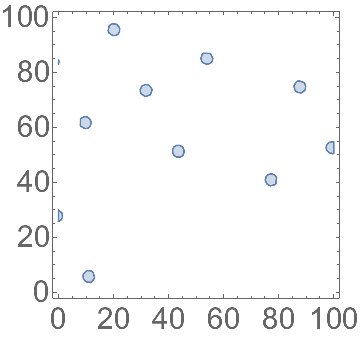
Figure 1: Feasible initial ${\phi}_{1}$ and ${\phi}_{2}$ under the constraints of Planck 2018 observation as shown in Table 1 are shown on the left. The $x$ axis and $y$ axis of both graphs correspond to the initial values of ${\phi}_{1}$ and ${\phi}_{2}$ in units of ${M}_{\text{pl}}$ respectively. For further investigation, we focus on the circle $9{M}_{\text{pl}}\leq{\phi}_{1}\leq 13{M}_{\text{pl}}$ and $3{M}_{\text{pl}}\leq{\phi}_{2}\leq 8{M}_{\text{pl}}$ as shown on the right.

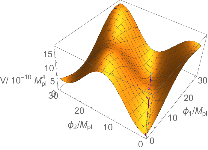
Figure 2: Natural inflation potential and field evolutions. The colours of the curves correspond to the parameters listed in Table 3.

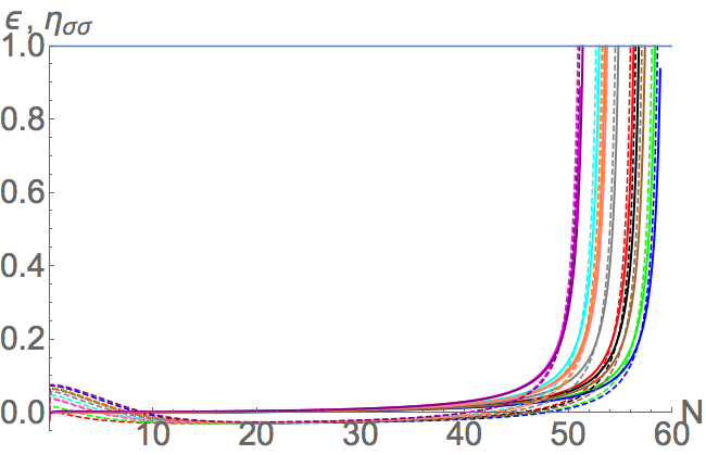
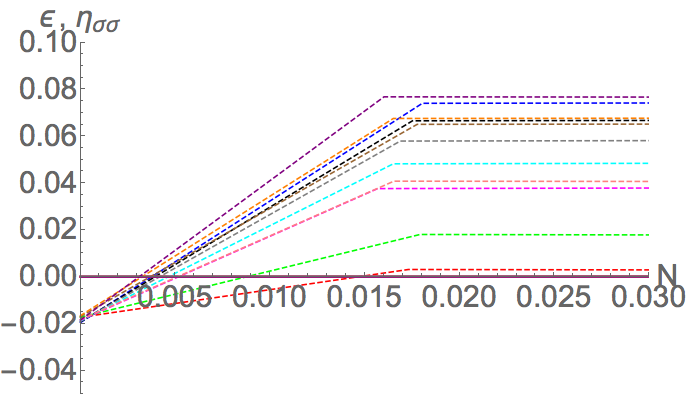
Figure 3: Evolutions of ${\epsilon}$ (solid lines) and ${\eta}$ (dashed lines) are shown on the left. The initial evolutions are shown on the right. Since all the parameter sets have small $\epsilon$ value at scales of about $O\left(10^{-9}\right)$, they overlap around the $x$ axis. Different colours correspond to the parameter sets listed in Table 3.

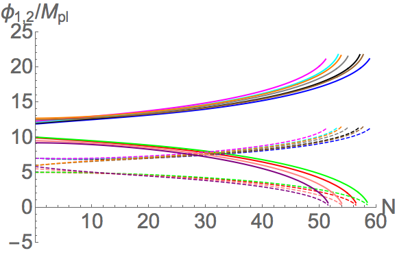
Figure 4: Field evolution as the number of e-foldings runs from $0$ to some values between $50$ and $60$. The solid lines correspond to the evolution of ${\phi}_{1}$ while the dashed lines correspond to that of ${\phi}_{2}$. The colours refer to the parameters listed in Table 3.

Next, we plot the evolutions of Hubble parameter under various parameter sets and initial conditions as shown in Figure 5. Starting from about $1.1\times 10^{-5}$, Hubble parameter initially decreases slowly and decreases significantly after about $30$ e-foldings. This matches with the observation constraint $\frac{H}{{M}_{\text{pl}}}<2.7\times 10^{-5}$ [3] and confirms our usual assumption that $H$ remains nearly constant during slow-roll approximation and ${\epsilon}=-\frac{\dot{H}}{H^{2}}$ gradually tends to $1$ as inflation ends. Furthermore, we plot the turn rate as shown in Figure 6. Basically, the turn rate initially drops quickly from about $0.07\sim 0.16$ to $0$. This implies that the inflation curve initially turns a little bit and moves along a straight line down to a trough without changing its direction, which matches with the inflation curves shown in Figure 2.

In addition, the evolutions of ${T}_{\mathcal{SS}}$ and ${T}_{\mathcal{RS}}$ against the number of e-foldings are plotted in Figure 7 and Figure 8. For ${T}_{\mathcal{SS}}$, starting from $1$, it decreases rapidly to reach nearly zero for the rest of the inflation process after $N=O\left(10^{-7}\right)$. Meanwhile, for ${T}_{\mathcal{RS}}$, starting from $0$, it rises significantly at a decreasing rate and remains stable after $N=O\left(10^{-7}\right)$. Finally, graphs of spectral indexes against the number of e-foldings are plotted in Figure 9. The evolutions initially have a sudden drop and they remain level between $0.96$ and $0.967$ after $N=O\left({10}^{-7}\right)$. Since the tensor-to-scalar ratio is given by $r\simeq\frac{16{\epsilon}\left({N}_{\text{hc}}\right)}{1+{T}_{\mathcal{RS}}\left({N}_{\text{hc}},N\right)^{2}}$ and ${\epsilon}=O\left(10^{-9}\right)$ in our model, it satisfies the latest Planck constraints [3]. Furthermore, ${\beta}_{\text{iso}}$ and $\cos{\Delta}$ evaluated from ${N}_{\text{hc}}$ to ${N}_{\text{end}}$ are listed on Table 3. Basically, we can see that ${\beta}_{\text{iso}}$ and $\cos{\Delta}$ have scales of at least $O\left(10^{-30}\right)$ and $O\left(10^{-4}\right)$ respectively, which satisfy the latest observation constraint ${\beta}_{\text{iso}}<9.5\times 10^{-4}$ and $-0.05\leq\cos{\Delta}\leq 0.05$.

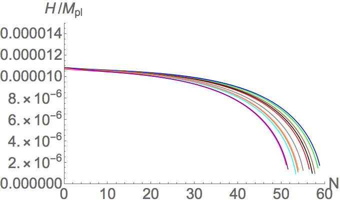
Figure 5: Evolution of Hubble parameter against the number of e-foldings. Starting from about $1.1\times 10^{-5}$, Hubble parameter initially decreases slowly and decreases significantly after about $30$ e-folding.

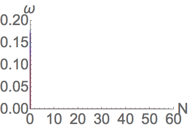
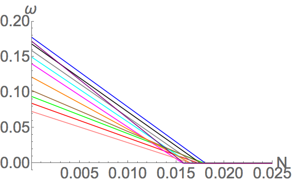
Figure 6: Turn rate against the number of e-foldings from $0$ to $60$ are shown on the left. The turn rate drops very quickly to $0$. On the right, one may see the initial evolutions of $\omega$, say, from $0$ e-folding to $0.04$ e-folding.

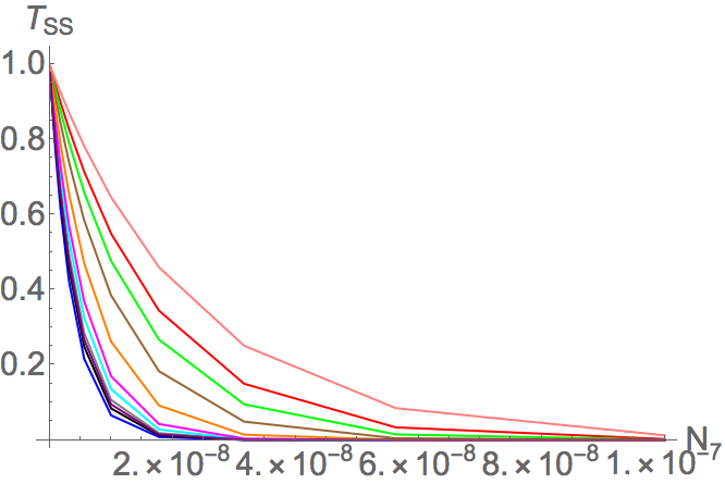
Figure 7: Evolutions of ${T}_{\mathcal{SS}}$ against the number of e-foldings are shown on the left. The graph on the left shows the evolutions for the whole inflation, while the graph on the right shows the initial evolutions.

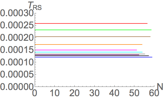
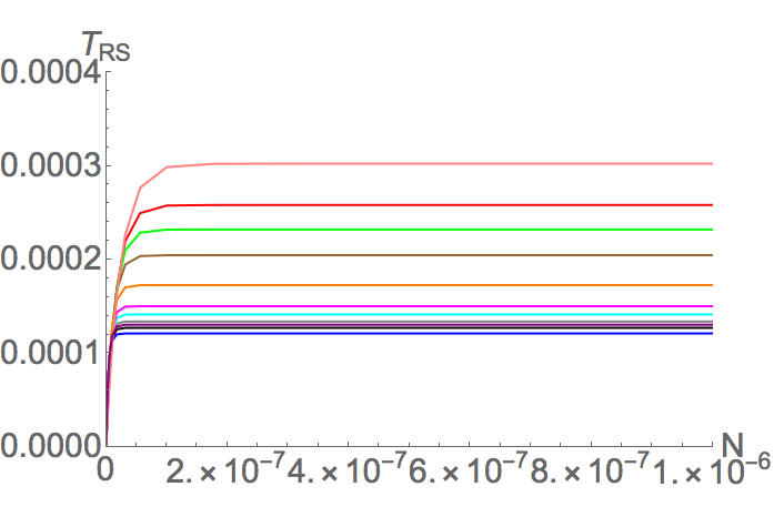
Figure 8: Evolutions of ${T}_{\mathcal{RS}}$ against the number of e-foldings are shown on the left. The graph on the left shows the evolutions for the whole inflation, while the graph on the right shows the initial evolutions.

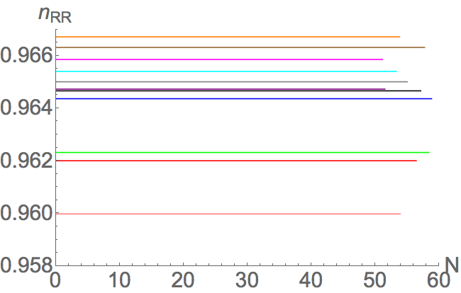
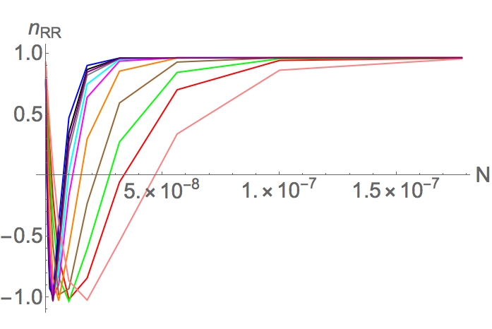
Figure 9: Evolutions of ${n}_{\mathcal{RR}}$ against the number of e-foldings. The graph on the left shows the evolutions for the whole inflation, while the graph on the right shows the initial evolutions.

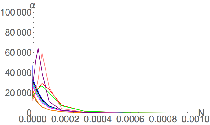
Figure 10: Evolutions of ${\alpha}$ against the number of e-foldings. The graph on the left shows the evolutions for the whole inflation, while the graph on the right shows the initial evolutions.

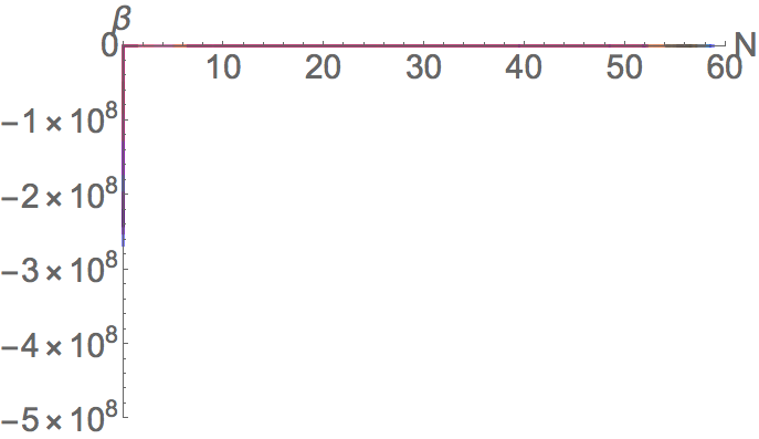
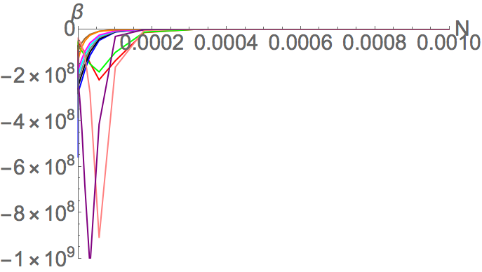
Figure 11: Evolutions of ${\beta}$ against the number of e-foldings. The graph on the left shows the evolutions for the whole inflation, while the graph on the right shows the initial evolutions.

5 Discussion

In this section, we try to explain some results listed above and make comments on them. First of all, about the smallness of $\epsilon$, this is because the initial velocities of field values are taken to be small. Now that we take the initial velocities at a scale of $O\left(10^{-5}\right)$, ${\epsilon}$ initially has a scale of about $O\left(10^{-9}\right)$. For example, if we replace the initial velocities at a scale of $O\left(10^{-3}\right)$, then ${\epsilon}$ initially has a scale of about $O\left(10^{-5}\right)$ instead, which also satisfies the latest Planck observation [3], and vice versa.

Next, one may see the evolutions of ${T}_{\mathcal{SS}}$ and ${T}_{\mathcal{RS}}$ change significantly at the beginning of inflation and remain constant during the inflation. To know the reasons, we should take a look at the evolutions of ${\alpha}\left(N\right)$ and ${\beta}\left(N\right)$ as shown in Figure 10 and 11. For the evolution of ${\alpha}\left(N\right)$, we can see that all curves decay rapidly and go to zero after $N=4\times 10^{-4}$. This makes ${T}_{\mathcal{RS}}$ initially surge and then remain level. The reason why ${\alpha}\left(N\right)$ have such a evolution is because the smallness of Hubble parameter at the beginning of inflation, which have a scale of $O\left(10^{-5}\right)$ as shown in Figure 5, contributes to a large scale, and the turn rate ${\omega}$ drops to zero after $N=0.02$ as shown in Figure 6. Similarly, for the counterpart of ${\beta}\left(N\right)$, we can see that all curves rise at a very fast rate starting from $-10^{9}$ to reach zero after $N=3\times 10^{-4}$. This makes ${T}_{\mathcal{SS}}$ decays rapidly and remains nearly zero after $N=10^{-7}$. Due to these two reasons, they make the spectral indexes suffer a sudden drop to about $-1$ and return to the range between $0.96$ and $0.967$ as shown in Figure 9. These parameter sets describe a scenario that the entropic perturbation mainly contribute to the adiabatic perturbation instead of self-preserving. Non-perturbative effects of supergravity and superstring theory can trigger inflation.

6 Conclusions and Future Work

In summary, we adopt the double field natural inflation model motivated by the non-perturbative effects of supergravity and superstring theory to do the slow roll analysis. We can see that under the constraints given by Planck observation there is freedom ($4{M}_{\text{pl}}$ for ${\phi}_{1}$ and $5{M}_{\text{pl}}$ for ${\phi}_{2}$) to choose the initial field values for inflation. This is in favour of our conjecture that quantum fluctuation causes the uncertainty of initial field values. Not only do they satisfy the Planck observation, but it also gives us some interesting physical ideas like how entropic perturbation contributes to adiabatic perturbation as supporting the universe to inflate. For the direction of further investigation, non-Gaussianity and double natural inflation with minimal and non-minimal coupling will be interesting. Double field natural inflation with non-canonical kinetic terms is also an interesting direction for further exploration. We also expect that more precise observations can be made so that stricter constraints can be attained to help us find the correct dynamics.

7 Acknowledgments

I thank Prof. Hiroyuki ABE very much for suggestion of my research, Dr. Hajime OTSUKA and Mr. Shuntaro AOKI for useful discussions related to field stabilisations and supergravity potential evaluations. I also want to express my sincere gratitude to Prof. Keiichi MAEDA for his opinions towards cosmological inflation analysis.

References

- [1] S. Carroll, Spacetime and Geometry: An Introduction to General Relativity, Addison Wesley, Pearson Education (2004).
- [2] D. Baumann, TASI Lectures on Primordial Cosmology (2017).
- [3] Planck Collaboration, et al, Planck 2018 results. X. Constraints on Inflation, arXiv: 1807.06211.
- [4] D.H. Lyth and A. Riotto, Particle physics models of inflation and the cosmological density perturbation, Phys. Rept. 314, 1 (1999), arXiv: hep-ph/9807278.
- [5] A. Mazumdar and J. Rocher, Particle physics models of inflation and curvaton scenarios, Phys. Rept. 497, 85 (2011), arXiv: 1001.0993.
- [6] David I. Kaiser, Edward A. Mazenc, and Evangelos I. Sfakianakis, Primordial Bispectrum from Multi-field Inflation with Non-minimal Couplings, Phys. Rev. D 87 (2013) 064004, arXiv: 1210.7487.
- [7] Katelin Schutz, Evangelos I. Sfakianakis and David I. Kaiser, Multifield inflation after Planck: iso-curvature modes from non-minimal couplings, Phys. Rev. D 89 (2014) 064044, arXiv: 1310.8285.
- [8] J. Maldacena, Non-Gaussian features of primordial fluctuations in single field inflationary models, JHEP 0305 (2003) 013, arXiv: astro-ph/0210603.
- [9] J. Hwang, H. Noh, Cosmological perturbations with multiple scalar fields, Phys. Lett. B 495 (2000) 277-283, arXiv:astro-ph/0009268.
- [10] C. Long, L. McAllister, P. McGuirk, Aligned Natural Inflation in String Theory, Phys. Rev. D 90 (2014) 023501.
- [11] Gordon, Christopher and Wands, David and Bassett, Bruce A. and Maartens, Roy, Adiabatic and entropy perturbations from inflation, Phys. Rev. D 63, 023506 (2000).
- [12] Christian T. Byrnes and David Wands, Curvature and iso-curvature perturbations from two-field inflation in a slow-roll expansion, Phys. Rev. D74, 043529 (2006).
- [13] Malik, K.A. and Wands, Cosmological perturbations, Phys. Rep. D. (2009) 475, 1, arXiv:0809.4944.
- [14] R. Kappl, H. P. Nilles, M.W. Winkler, Natural Inflation and Low Energy Supersymmetry, Phys. Lett. B 746 (2015) 15-21, arXiv: 1503.01777.
- [15] Rolf Kappl, Hans Peter Nilles, Martin Wolfgang Winkler, Modulated Natural Inflation, Phys. Lett. B, Vol. 753, (2016) 653-659, arXiv: 1511.05560f.
- [16] M. Grana, Flux Compactifications in String Theory: a Comprehensive Review, Phys. Rep. 423 (2006) 91-158, arXiv: hep-th/0509003.
- [17] S. Kachru, R, Kallosh, A. Linde, S. P. Trivedi, De Sitter Vacua in String Theory, Phys. Rev. D 68 (2003) 046005, arXiv: hep-th/0301240.
- [18] R. Kallosh, A. Linde, B. Vercnocke, Natural inflation in supergravity and beyond, Phys. Rev. D 90 (2014) 041303, arXiv: 1404.6244.
- [19] D. Z. Freedman, A.V. Proeyen, Supergravity, Cambridge University Press (2012), ISBN 978-0-521-19401-3.
- [20] H. K. Suonio, Cosmological Perturbation Theory, part 2 (2015).
- [21] Peccei, R.D., Quinn, H.R., CP conservation in the presence of pseudoparticles, Phys. Rev. Lett. 38 (1977) 1440.
- [22] Peccei, R.D., Quinn, H.R., Constraints imposed by CP conservation in the presence of pseudoparticles, Phys. Rev. D 16 (1977) 1791 75.