A simple method to determine the time delays in presence of microlensing: application to HE 0435-1223 and PG1115+080

Abstract

A method for determining the time delays in gravitationally lensed quasars is proposed, which offers a simple and transparent procedure to mitigate the effects of microlensing. The method is based on fundamental properties of representation of quadratically integrable functions by their expansions in orthogonal polynomials series. The method was tested on the artificial light curves simulated for the Time Delay Challenge campaign TDC0. The new estimates of the time delays in the gravitationally lensed quasars HE 0435-1223 and PG 1115+080 are obtained and compared with the results reported by other authors earlier.

1 Introduction

One of the potential astrophysical applications of measuring the differential time delays in gravitationally lensed quasars is a possibility to determine the Hubble constant value with no need of the intermediate standard candles. This was noticed for the first time by S.Refsdal (1964) long before the discovery of the first gravitationally lensed quasar, QSO 0957+561 (Walsh, Carswell & Weymann 1979). Knowledge of the time delays is necessary for many other applications in astrophysics and cosmology, such as studies of matter distribution at different spatial scales in the Universe, including the dark matter, investigation of spatial structures of lensing galaxies, etc.

The first attempt to measure the time delay has been made for QSO 0957+561 (Florentin-Nielsen 1984). Multiple further attempts provided noticeably diverging values for the time delay in this doubly imaged quasar (Schild & Cholfin 1986; Vanderriest et al. 1989; Press, Rybicki & Hewitt 1992), thus demonstrating complexity of the problem. This is due to a number of objective factors, such as: small amplitudes of the quasar intrinsic brightness variations, which are often comparable with the photometry errors; presence of microlensing events; the random flux transfer between the components in photometry of blended images; difficulties in providing the long-term uninterrupted monitoring with a sufficient sampling rate and high photometric precision. The detailed list of these factors can be found, e.g., in Tewes, Courbin & Meylan (2013). As a result, a consensus about the time delay value in the lens QSO 0957+561 was attained as late as in 1997 (Kundič et al. 1997; Schild & Thompson 1997).

During 1980-1992, fundamentals of determining the time delays in gravitationally lensed quasars has been elaborated (Press et al. 1992; Pelt et al. 1994). In the next years several methods to measure the time delays have been proposed based, in one form or another, on the approach developed in these pioneer works, (Schechter et al. 1997; Barkana 1997; Burud et al. 2000; Kochanek et al. 2006; Eulaers & Magain 2011; Courbin et al. 2011; Tewes et al. 2012, and other). In recent years, an increasing interest to the problem of measuring the time delays is observed from the astronomical community. To a considerable degree, this is caused by expectations of a huge data flow on the newly discovered strong lenses from the Dark Energy Survey, PanSTARRS, LSST and other survey programs when they become operational. In spite of a possible bias in the determination of the Hubble constant from the time delay technique due to the mass-sheet degeneracy (Falco et al. 1985; Xu et al. 2015), it is believed to be an important tool in cosmological studies.

Estimation of the Hubble constant from the time delays requires them to be measured with a rather high precision: according to Kochanek & Schechter (2004) the relative error of the order of 1% is needed. Until recently, the precision of time delay measurements was as a rule much lower. During the last few years, the situation is tending clearly to change. Thanks to the efforts of some targeted programs (e.g. COSMOGRAIL), the well-sampled light curves of a long duration and with rather short gaps between the seasons appeared for some objects and became publicly accessible, (e.g. Courbin et al. 2011; Eulaers et al. 2013; Rathna Kumar et al. 2013; Tewes et al. 2013). This has given rise to creation of new methods and versions of the already existing ones. Liao et al. (2015) report about seven teams participating in a blind signal processing competition named Time Delay Challenge 1 (TDC1), who submitted results from 78 different methods. They note that in processing their mock light curves, several methods have given the accuracy of $\leq 0.03$, while some of the methods have already reached sub-percent accuracy.

A family of methods known as the point estimators does not provide in a direct and explicit form the estimates of errors of determining the time delays, which would be an immediate output of processing the light curves. To obtain the time delay error estimate, an additional procedure is usually used, known as Monte Carlo simulation. In some works, e.g., Morgan et al. (2008), Hojjati et al.(2014), a statistical approach based on Gaussian process modeling is used. The approach does not need Monte Karlo simulation to estimate the error of the time delay determination and provides its own estimate of the uncertainty as a natural result of the whole procedure.

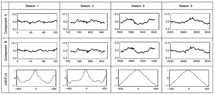
Figure 1: Synthetic TDC0 light curves ”rung2-pair4” and their regressions by series expansion in Legendre polynomials of the 39-th order (two upper rows), and the corresponding cross-correlation functions LNCF($\tau$) calculated according to Eq. 3. The data points, which are more than 3$\delta_{appr}$ offset from the regression curve are indicated by the open circles.

Most of methods needs some algorithms to build a model light curve. In doing so, a necessity arises to properly interpolate the unevenly sampled data points in the light curves under consideration, and this is one of the main technical problems in determining the time delays. A variety of interpolating functions and algorithms is used, such as polynomial approximation (Lehar et al. 1992; Kochanek et al. 2006), spline interpolation (Tewes et al. 2013b; Barkana 1997), smoothing with the sampling function (Vakulik et al. 2009) or with a linear combination of Gaussian kernels, (Cuevas-Tello, Tino & Raychaudhury 2006).

All these approaches, while differing in algorithms of the initial data interpolation, use, in one form or another, the cross-correlation maximum or mutual dispersion minimum criteria to find the time delay estimate. In some cases, the light curves of the lensed components are analysed in pairs, while sometimes, for example, for multiply imaged systems, the values of the time delays are determined from a joint analysis of light curves of all image components.

One of the most serious complications in time delay determination is due to microlensing events, which distort the intrinsic quasar light curves differently in different quasar images. The choice of a method to eliminate the effect of microlensing in each specific case depends strongly on characteristics of the quasar intrinsic variability and the variability caused by microlensing, in particular, on relationship between the typical amplitudes and time scales of both processes. The work by the participants of the COSMOGRAIL project (Tewes, Courbin & Meylan 2013) is dedicated to elaboration of methods for determining the time delays in presence of ”slow” microlensing events, that is, the events with the characteristic time scale of variability exceeding that of the quasar variability.

2 The proposed method

Our approach to determine the time delays implies a pair-wise comparison of light curves, with both of them represented by their polynomial regressions. To approximate the initial light curves, we use their representations as the series expansions in orthogonal polynomials.

2.1 Regression procedure

Approximations and series expansions in normalized orthogonal functions are known to possess a number of useful properties, (Korn & Korn 2000, Secs.15.2-6, 20.6-2), which provide certain convenience and flexibility in practice. In particular, approximation of an arbitrary quadratically integrable function $f(x)$ by an orthonormal set, say, $u_{0}(x),\,u_{1}(x),\,u_{2}(x),\,...,\,u_{n}(x)$ of the form $f(x)\approx s_{n}(x)=a_{0}u_{0}(x)+a_{1}u_{1}(x)+a_{2}u_{2}(x)+...+a_{n}u_{n}(x)$ has the advantage that exclusion of some terms from the sum $s_{n}(x)$ or addition of a new extra term $a_{n+1}u_{n+1}(x)$ leave the values of previously computed coefficients $a_{0},a_{1},a_{2},...,a_{n}$ unchanged.

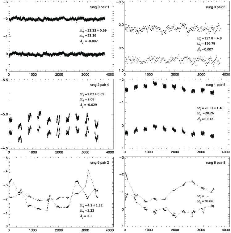
Figure 2: Some results of participation in a Time Delay Challenge (TDC0) campaign. Six pairs of the simulated light curves of various types are presented. The quantities in the panels are: the time delay estimates $\Delta t^{\prime}_{j}$ determined with the use of the proposed method and the corresponding uncertainties $\delta_{j}$ calculated as described in Sec. 2; the true time delays $\Delta t_{j}$, and the relative deviations of particular estimates from the corresponding true values, $A_{j}={{\Delta t^{\prime}_{j}-\Delta t_{j}}\over\Delta t_{j}}$, – ”accuracy” or ”bias” of an individual determination according to Liao et al. (2015).

In the works of some authors, for example, Kochanek et al. (2006), Lehar et al. (1992), Legendre polynomials are used, which are orthogonal only at the continuous set of points specified in a finite interval with a constant weighting function. To make use of the advantages of the orthogonal-polynomial regressions, we must start from constructing an orthonormal basis specified at a discrete set of unevenly spaced data points (the dates of observations in our case). Such a basis can be constructed through the Gram-Schmidt orthogonalization procedure (Korn & Korn 2000, 15.2-5). Any arbitrary set that represents a complete function system specified at the dates of observations can be accepted in this procedure as an initial basis. In our case, the system of Legendre polynomials turned out to be the best one in the sense of computational stability.

In a general case, if $f(x)$ is given at a discrete set of $m+1$ points $x_{0},\,x_{1},...,\,x_{m}$, the coefficients $a_{i}$ in $s_{n}(x)$ are determined (Korn & Korn 2000, 20.6-2) by the expression:

$$a_{i}={{\sum_{k=0}^{m}\gamma_{k}f(x_{k})u_{i}(x_{k})}\over{\sum_{k=0}^{m}\gamma_{k}u_{i}^{2}(x_{k})}}$$ (1)

where $\gamma_{k}$ are the weights, which are related to photometric uncertainties and often put to equal unity, and $i=0,1,2,...,n,(n\leq m)$.

The property indicated above provides a very simple procedure to exempt the light curves of the lensed quasar components from the effects of microlensing events, at least for those lenses where the microlensing brightness variations are much slower as compared to the quasar intrinsic brightness fluctuations. Making use of the properties of the orthonormalized polynomials noted above, we may exclude for such lenses the lower-order terms from a series approximating the light curve of a certain image component without a necessity to recalculate coefficients of the polynomial regression. In doing so, we remove the linear (or quadratic if needed) trends inherent both in microlensing and in the intrinsic variability of a quasar. Besides, we obtain the light curve representations all reduced to the zero average level. Naturally, we may return these lower-order terms, thus recovering the average level for each component and, if needed, using them to represent the microlensing light curves without any additional calculations.

There may be the data points in the observed light curves, which are offset from the regression curve by a quantity exceeding noticeably both the RMS error of photometry $\delta_{phot}$ and the approximation error, $\delta_{appr}$, which is the RMS deviation of the data points from the polynomial regression calculated and displayed in running the program. We permitted that up to two or three data points, which are more than 3$\delta_{appr}$ offset from the regression curve, be identified by the program. Then these points get the values inherent in the regression curve in their locations, and the approximation routine is repeated with the data points modified in this way.

To select the maximal ”reasonable” order of the polynomial regression, we were guided, on one hand, by a behaviour of the RMS errors of approximation in its dependence on the polynomial order. In particular, the error of approximation $\delta_{appr}$ must be close to the error typical of the initial photometry data, $\delta_{phot}$, but must not exceed it: $\delta_{appr}\leq\delta_{phot}$. On the other hand, oscillations in the regression curves emerging sometimes at the ends of observational seasons, must not exceed the photometry errors in amplitudes. This may serve as a constraint on the upper limit of the polynomial order.

2.2 Calculation of cross-correlations and uncertainties

The further analysis consists in calculation of the cross-correlation function CF$(\tau)$ for a corresponding pair of light curves represented by the values of their polynomial regressions $f(t_{k})$ and $g(t_{k})$ in the evenly sampled data points:

$$CF(\tau)={1\over M}\sum_{k}{{[f(t_{k})-f^{*}][g(t_{k}+\tau)-g^{*}]}\over{\sqrt{D_{f}D_{g}}}}$$ (2)

Here, $f(t_{k})$ and $g(t_{k})$ are the values of the approximating polynomials in the corresponding points, $f^{*}$ and $g^{*}$ are their mean values at the considered interval, $\tau$ is the time lag, $M$ is a number of common points in $f(t_{k})$ and $g(t_{k})$, which participate in calculations of $CF(\tau)$, and $D_{f}$, $D_{g}$ are variances of $f(t_{k})$ and $g(t_{k})$.

As one data set slides across the other in calculating the cross-correlation function, the data points near the signal edges fall out of the calculations successively, thus resulting in distortion of the cross-correlation function. To exclude such edge effects, we used a cross-correlation procedure similar to the Locally Normalized Discrete Correlation Function, (LNDCF), proposed by Lehar et al. (1992). Namely, we replaced the mean values $f^{*}$ and $g^{*}$ and their variances $D_{f}$ and $D_{g}$ with their current values $f^{*}_{\tau}$ and $g^{*}_{\tau}$, $D_{f\tau}$ and $D_{g\tau}$ corresponding to the given time lags $\tau$:

$$LNCF(\tau)={1\over M_{\tau}}\sum_{k}{{[f(t_{k})-f^{*}_{\tau}][g(t_{k}+\tau)-g^{*}_{\tau}]}\over{\sqrt{D_{f\tau}D_{g_{\tau}}}}}$$ (3)

For this Locally Normalized Correlation Function, LNCF$(\tau)$, the program is searching for the maximum, and its position is then accepted as an estimate of the time delay for a particular image pair.

In estimating the uncertainties $\delta_{j}$ of our time delay measurements, we do not use the Monte Carlo simulation, but proceed in the following way. The estimates of statistical parameters of a stationary random process are known to be equally valid both from the analysis of the whole signal record, and by averaging the results of processing separate realizations (subsets) of the process. Therefore, we accept the estimates of the time delays for individual seasons averaged over the seasons as the most probable values of the time delays. The RMS deviation of the time delays for separate seasons from their average over the seasons is proposed to be treated as a measure of uncertainty $\delta_{j}$ of a particular time delay determination.

In Fig. 1 we show some examples of the synthetic light curves proposed to the astronomical community by the Time Delay Challenge (TDC) campaign (Liao Kai et al. 2015). The light curves ”rung2-pair4” of the TDC0 issue and their regressions by expansions in Legendre polynomial series calculated in the way described in Sec. 2 are presented for four seasons, as well as the corresponding cross-correlation functions LNCF($\tau$) calculated according to Eq. 3.

3 Testing the method: processing the mock light curves

The goal of the TDC campaign was to let the researches check their capability to quickly and adequately process and interpret a huge flow of the observational data expected from the Dark Energy Survey, PanSTARRS, and LSST, when they become operational. We used the TDC0 synthetic light curves to test our method for precision, bias and robustness.

At the first stage of the competition, TDC0, 56 pairs of time series have been issued, from the most simple cases – low-noise, well-sampled time series, without seasonal gaps and microlensing, – and those ones poorly sampled, with large gaps and distorted by the effects of noise and microlensing events. The simulation team proposed four metrics (Liao et al. 2015, Dobler et al. 2015), which serve as criteria for the participants to pass the TDC0 stage. One of them is efficiency, $f$, quantified as a fraction of light curves, for which the estimates are obtained. Three other metrics are the goodness of fit quantified by the value of $\chi^{2}$, and, according to terminology by Liao et al. (2015), the ”precision” of the estimator $P$ and the ”accuracy” or ”bias” $A$:

$$\chi^{2}={1\over{fN}}\sum_{j}\left({{\Delta t^{\prime}_{j}-\Delta t_{j}}\over\delta_{j}}\right)^{2},$$ (4)

$$P={1\over{fN}}\sum_{j}\left({\delta_{j}\over{|\Delta t_{j}|}}\right),$$ (5)

$$A={1\over{fN}}\sum_{j}\left({{\Delta t^{\prime}_{j}-\Delta t_{j}}\over\Delta t_{j}}\right)$$ (6)

Here, $N$ is a total number of the proposed light curves, $\Delta t^{\prime}_{i}$ are the time delay values determined by the participants, with their uncertainties $\delta_{j}$, and $\Delta t_{j}$ are the true time delays.

The simulation team selected the following criteria to pass the TDC0: $f>0.3$, $0.5<\chi^{2}<2$, $P<0.15$, and $A<0.15$. We were not cautious enough in selecting the results for submission, having included some ambiguous measurements of the time delays, or the measurements with too large values of the estimated uncertainties. This resulted in $f=0.64$ and, quite naturally, in inadmissibly large values of $P$ and $A$. Meanwhile, rejection of even a few uncertain results leads to the abrupt changes in values of the metrics. In the further analysis presented below, we addressed our results corresponding to $f=0.54$, (a number of successful determinations is 30). It means that, as compared to the results submitted to the TDC0 ”evil team”, we excluded from the present analysis six determinations for which the individual relative errors $P^{\prime}_{j}={\delta_{j}/\Delta t^{\prime}_{j}}$ more than three times exceeded the average relative error $P^{\prime}$ for the sample under investigation:

$$P^{\prime}={1\over{fN}}{\sum_{j}\left({\delta_{j}\over|\Delta t^{\prime}_{j}|}\right)}\,.$$ (7)

Therefore, we rejected the uncertain determinations blindly, that is, we did not address the true time delays, but used the quantities $P^{\prime}_{j}={\delta_{j}/\Delta t^{\prime}_{j}}$ and (7); the latter is called the ”blind” precision in Bonvin et al. (2016).

Table 1: The metrics A, P and $\chi^{2}$ (Eqs.4 - 6) calculated for three different ranges of the time delays: the short delays, $\Delta t<10$, medium, $10<\Delta t<50$, and long ones, $\Delta t>50$. In the last column, the metrics for all the three subsets calculated together are presented. The last line shows the subsample sizes used in estimating the metrics.

Metrics	$\Delta t<10$	$10<\Delta t<50$	$\Delta t>50$	All
P	$1.03\pm 0.74$	$0.14\pm 0.08$	$\,\,0.05\pm 0.04$	$0.39\pm 0.40$
A	$0.24\pm 0.17$	$0.05\pm 0.07$	$-0.04\pm 0.06$	$0.09\pm 0.11$
$\chi^{2}$	$0.38\pm 0.27$	$0.62\pm 0.66$	$\,\,5.75\pm 6.22$	$1.91\pm 2.57$
Number	9	13	8	30

Table 2: Robustness test fulfilled for three different groups of the time delay values corresponding to the short, medium and long delays (according to the ranges indicated in Table 1). Our estimates $\Delta t^{\prime}_{j}$ with the corresponding uncertainties $\delta_{j}$, their deviations from the true values $\Delta t^{\prime}_{j}-\Delta t_{j}$, and the corresponding relative deviations, $A_{j}={{\Delta t^{\prime}_{j}-\Delta t_{j}}\over\Delta t_{j}}$, are shown for three modes of sampling the light curves.

Sampling mode	$\Delta t^{\prime}_{j}\pm\delta_{j}$	$\Delta t^{\prime}_{j}-\Delta t_{j}$	$A_{j}$
True time delay $\Delta t=2.08$ (rung2-pair4)
Original set	2.02$\pm$ 0.09	-0.06	-0.030
Each 5-th point omitted	2.09$\pm$ 0.09	0.01	0.005
Each 3-rd point omitted	2.05$\pm$ 0.19	-0.03	-0.014
True time delay $\Delta t=28.73$ (rung1-pair8)
Original set	28.48$\pm$ 3.66	-0.25	-0.009
Each 5-th point omitted	27.96$\pm$ 4.43	-0.77	-0.027
Each 3-rd point omitted	28.89$\pm$ 3.84	0.16	0.006
True time delay $\Delta t=156.78$(rung3-pair6)
Original set	157.8$\pm$ 13.4	1.02	0.007
Each 5-th point omitted	163.4$\pm$ 18.9	6.62	0.041
Each 3-rd point omitted	158.4$\pm$ 7.4	1.62	0.010

In testing the method in terms of the metrics (4)-(6), we dealt with the TDC0 set consisting of the light curves of several types, which differ in their amplitudes, signal-to-noise ratios, sampling rates, and contributions from microlensing. Also, in preparing our determinations for submission, we could not but notice that short time delays demonstrate in general worse precision as compared to the long and medium ones. As the simulation team commented in the reply to our submission, it was typical of many of the submissions. Therefore, we analysed the metrics for the short, medium and long time delays separately.

We calculated the quantities $A$, $P$ and $\chi^{2}$ determined by expressions (4-6) for the following subsets of the submitted light curves differing in ranges of $\Delta t_{j}$: for $\Delta t_{j}\leq 10$ (short delays), $10\leq\Delta t_{j}\leq 50$ (medium), and $\Delta t_{j}>50$, (long delays). The results are shown in Table 1. For the short time delays, $\Delta t_{j}\leq 10$, the values of $A$ and $P$ exceed the boundaries of the TDC0 criteria, while $\chi^{2}$ is noticeably less than permitted that can be explained by overestimation of the uncertainties $\delta_{j}$. For $10\leq\Delta t_{j}\leq 50$, all the three metrics meet the TDC0 criteria. And finally, for the longest time delays we have $A=-0.04$ and $P=0.05$, while $\chi^{2}$ turns out to be too large. This can be explained by the presence of a single determination in this subsample, which deviates from the true time delay by the quantity exceeding the estimated error $\delta_{j}$, (this is, in particular, ”rung3-pair5” light curves: $\Delta t^{\prime}_{j}-\Delta t_{j}=5.26$, while the estimated $\delta_{j}=0.9$).

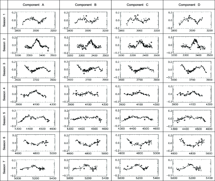
Figure 3: Light curves of HE 0435-1223 and their approximations by series expansions in Legendre polynomials (image components from A to D are from left to right, seasons 1-7 from top to bottom); the low-order terms are excluded. The ”bad” points (see in the text) are marked by squares. The Heliocentric Julian Dates reduced by 2450000 days (HJD-2450000) are along the horizontal axis.

Table 2 demonstrates some results of testing our method for robustness. Again, the cases of short, medium and long time delays were considered separately. The table contains our estimates of the time delays $\Delta t^{\prime}_{j}$ with their errors $\delta_{j}$ calculated in the way described in Section 2.2, deviations of our estimates from the true values, $\Delta t^{\prime}_{j}-\Delta t_{j}$, and the corresponding relative deviations $A_{j}=(\Delta t^{\prime}_{j}-\Delta t_{j})/\Delta t_{j}$, (individual signed ”accuracies”, or ”biases”). These values were calculated for three modes of sampling the light curves: the original data, as they have been proposed for TDC0, the light curves with each fifth point omitted, and those with each third point omitted.

Thus, the method is resistant to exclusion of up to 33% of the light curve data points, at least for the considered cases. The degree of robustness is understood to depend on the mode of the initial data sampling, and on the signal-to-noise ratio inherent in the initial data photometry.

Closing consideration of the metrics for our estimator, we would like to note that in 6 cases of 30 successful determinations, the relative deviations from the true delay values $A_{j}$ less than 0.01 have been achieved. As to the failures, their largest amount took place for the most difficult (while most realistic) cases of sparse and noisy data points, with large gaps, as well as with strong and fast microlensing events, (”rung5” and ”rung6” sets). In Fig. 2 six different types of the simulated light curves are shown together with our determinations of the time delays $\Delta t^{\prime}_{j}$ and their uncertainties $\delta_{j}$, true time delays $\Delta t_{j}$, and the corresponding relative deviations of our estimates from the true values $A_{j}=(\Delta t^{\prime}_{j}-\Delta t_{j})/\Delta t_{j}$. We see two cases of very successful hits here, with $A_{j}<0.01$, as well as one of the examples of our failures (”rung6-pair8” curves).

4 Quadruple lens HE 0432-1223

We applied our method to the excellent data of the 7-years monitoring of the quadruple gravitation lens HE 0435-1223 (the photometry is available from the CDS archive, http://cdsarc.u-strasbg.fr/), which have been used by Courbin et al. (2011) to determine the time delays.

Table 3: The estimates of the time delays $\Delta t$ (in days) for all the six component pairs of the HE 0435-1223 quadruple system, as measured by Kochanek et al.(2006) and Courbin et al. (2011), (the data are taken from the latter work).

Data	Author	$\Delta t_{AB}$	$\Delta t_{AC}$	$\Delta t_{AD}$	$\Delta t_{BC}$	$\Delta t_{BD}$	$\Delta t_{CD}$
SMARTS(seasons 1,2)	Kochanek(2006)	-8.0$\pm 0.8$	-2.1$\pm 0.8$	-14.4$\pm 0.8$
SMARTS(seasons 1,2)	Courbin(2011), MD	-8.8$\pm 2.4$	-2.0$\pm 2.7$	-14.7$\pm 2.0$	6.8$\pm 2.7$	-5.9$\pm 1.7$	-12.7$\pm 2.5$
COSMOGRAIL,7 seasons	Courbin(2011), MD	-8.4$\pm 2.1$	-0.6$\pm 2.3$	-14.9$\pm 2.1$	7.8$\pm 0.8$	-6.5$\pm 0.7$	-14.3$\pm 0.8$

Table 4: The time delay values (in days) for HE 0435-1223 as determined from different seasons with the proposed method. For each time delay the value of the corresponding cross-correlation function in its maximum is indicated in brackets.

Season	$\Delta t_{AB}$	$\Delta t_{AC}$	$\Delta t_{AD}$	$\Delta t_{BC}$	$\Delta t_{BD}$	$\Delta t_{CD}$
Season 2 (2005)	-11.0 (0.974)	-0.8 (0.988)	-14.5 (0.983)	10.4 (0.995)	-3.7 (0.989)	-14.7 (0.996)
Season 3 (2006)	-10.2 (0.967)	-2.3 (0.990)	-11.9 (0.974)	7.2 (0.968)	-3.3 (0.978)	-9.5 (0.961)
Season 4 (2007)	-10.9 (0.807)	-3.8 (0.934)	-13.1 (0.931)	3.4 (0.891)	-9.1 (0.893)	-10.4 (0.946)
Season 5 (2008)	-10.6 (0.556)	-5.0 (0.963)	-21.3 (0.871)	7.2 (0.603)	-9.4 (0.771)	-15.3 (0.915)
Season 6 (2009)	-10.0 (0.980)	-2.7 (0.957)	-5.8 (0.950)	5.2 (0.942)	-3.4 (0.956)	-1.6 (0.943)
Average	$-10.3\pm 0.4$	$-2.9\pm 1.4$	$-13.3\pm 3.7$	$6.7\pm 2.3$	$-5.8\pm 2.8$	$-10.3\pm 3.5$
Season 1 (2004)	-1.6 (0.963)	1.4 (0.829)	-18.5 (0.965)	-0.4 (0.840)	-22.1 (0.915)	-20.7 (0.910)
Season 7 (2010)	-1.6 (0.966)	0.0 (0.954)	-1.4 (0.951)	1.3 (0.977)	2.9 (0.949)	-0.2 (0.964)

The lens HE 0435-1223 is an example of the systems where microlensing events can be considered as ”slow” ones. The object with a redshift of $z=1.689$ was identified as a quasar lensed by a $z=0.4546$ galaxy by Wisotski et al. (2002). The first time delay estimates have been made by Kochanek et al.(2006) from the two-years monitoring data obtained in 2004-2005 with the SMARTS 1.3-m telescope. Later on, these data were supplemented by observations at other telescopes, and observations in 2006-2010 have been added (Courbin et al. 2011). The estimates of the time delays obtained in these two works are shown in Table 3 taken from Courbin et al. (2011).

To describe the intrinsic variability of a source quasar, Kochanek et al. (2006) approximated the data by series expansion in Legendre polynomials, with the A component selected as the reference one. The maximum permissible order of the polynomial was determined with the use of the F-test and constituted 20. The microlensing brightness variations in individual images with respect to image A (differential microlensing) were described separately by Legendre series as well, but of much lower orders - 3 or less. Thus, the model light curve was composed of two constituents: the quasar light curve approximated as a Legendre series of the order up to 20, and microlensing variations represented as a lower-order Legendre series. Then the problem of searching the parameters is solved, which would provide the minimal RMS difference between the observed light curve and the reference (model) one built in the way described above. The data of each season were processed separately. The results taken with this approach are presented in Table 3 (the first line).

The second and third lines in Table 3 contain the time delays of HE 0435-1223 obtained by Courbin et al. (2011) from the results of the detailed seven-years monitoring. The approach used in their work is based on the minimum dispersion (MD) method proposed by Pelt et al. (1996). To avoid the effect of the reference curve selection, each pair was processed twice, with the change of the reference component. Then the total dispersion was minimized by varying the time lags and parameters of the polynomials representing microlensing light curves. According to Courbin et al. (2011), variations of the quasar brightness were least of all distorted by microlensing in component B.

The light curves of the A, B, C and D image components and the corresponding regression curves calculated according to the algorithm described in Sec. 2 can be seen in Fig. 3. Two low-order terms (the mean level and linear trend) were excluded to represent the source quasar light curves in seasons 1 to 3 and 6 to 7, while for seasons 4 and 5 the next (quadratic) term was also needed to represent microlensing, therefore, three lower-order terms were excluded from the light curves in Fig. 3 for these seasons.

The orders of polynomials were 17 for the 2-nd season, 15 for the 4-th and 5-th ones, and 11 for the rest. As is noted in Section 2, in selecting the polynomial order, we were guided, first, by a behavior of the RMS error of approximation in its dependence on the polynomial order, and second, we tried to avoid oscillations emerging sometimes for too high orders. An increase of the polynomial order above 17 was found to have a minor effect on the precision of approximation while producing unacceptable oscillations at the realization borders. It should be noted that season 2 is characterized, as compared to others, by the most fast and high-amplitude variations of flow, thus providing the highest reliability of the time delay estimates.

The next step was the calculation of the Locally Normalized Correlation Functions (LNCF) for the pairs of approximating polynomials exempted from the lower-order terms representing the ”slow” microlensing. The examples of such cross-correlation functions calculated for all the six permutations of four components in two are presented in Fig. 4 (the data of the second and fifth seasons were used as the examples of the ”best” and ”worst” seasons in the sense of their cross-correlation maxima values).

The estimates of the time delays for all seasons are shown in Table 4, together with the results of their averaging over the seasons. The values of the corresponding cross-correlation functions in their maxima are shown in brackets. The errors indicated in Table 4 in the ”Average” line were calculated as the RMS deviations of the values obtained for each season from the value averaged over all seasons (see Sec. 2.2 for more explanations).

Table 5: Values of the time delays in PG1115+080 (in days) from observations by Schechter et al., presented in Schechter et al. (1997), Barkana 1997, Eulaers et al. (2011), and from observations at the Maidanak Observatory in 2004-2006 (Vakulik et al. (2009). In the last two lines, the results of re-analysis fulfilled in this work are presented .

Authors	$\Delta t_{BA}$	$\Delta t_{CA}$	$\Delta t_{BC}$	Comments
Schechter et al.(1997)	14.3$\pm$3.4	9.4$\pm$3.4	23.7$\pm$3.4	Method by Press et al. (1992)
Barkana (1997)	11.7$\pm$2.0	11.0$\pm$0.9	25.0$\pm$3.6	Method by Press et al. (1992)
Eulaers & Magain(2011)	5.8	15	20.8	Numerical Model Fit (NMF)
Eulaers & Magain(2011)	10.3	7.6$\pm$3.9	17.9$\pm$6.9	Minimum Dispersion Method ((MD)
Vakulik et al.(2009)	4.4$\pm$3.2	12.0$\pm$2.4	16.4$\pm$3.4	Joint estimate over three seasons
Vakulik et al.(2009)	5.0	9.4	14.4	For the first season
This work	12.9	4.2	16.8	For the first season
This work	9.7$\pm$2.5	7.5$\pm$5.3	17.6$\pm$6.9	Averaged over three seasons

First of all, a very good convergence of estimates for the AB pair between the seasons should be noted, with the uncertainty as small as 0.4 days, though the time delay values themselves are systematically larger than those in (Kochanek et al. 2006) and (Courbin et al. 2011). Somewhat larger uncertainty, though smaller than that in Courbin et al. (2011), is observed for the AC pair, with the time delay value consistent with those in Table 3. The rest of the pairs demonstrate noticeably larger scatter between the seasons, while the average estimates are rather well consistent with the results reported by Kochanek et al. (2006) and Courbin et al. (2011), excluding, perhaps, the CD pair. And finally, a very poor consistence of the results for seasons 1 and 7 with those for other seasons should be noted for all the component pairs. The reason may be a somewhat worse photometry and/or more sparse sampling of the initial light curves, as compared to other seasons. Surprisingly, it is not always confirmed by the values of the cross-correlation maxima indicated in the brackets.

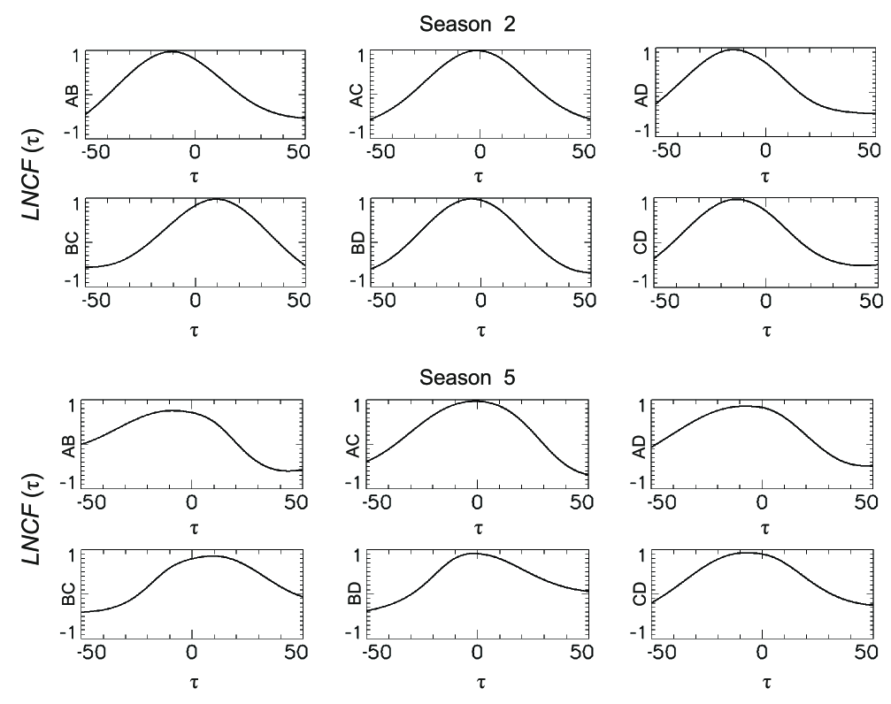
Figure 4: Locally normalized cross-correlation functions $LNCF(\tau)$ for pairs of the HE 0435-1223 light curves represented by the regressions shown in Fig.3 (seasons 2 and 5).

Courbin et al. (2011) report that they tested their curve-shifting method for stability in different ways, in particular, by processing separate seasons and groups of seasons. In doing so, they found out no effect on the result that would be of any significance (unfortunately, the time delay values for individual seasons are not presented in their paper). They also note that stability of estimations will be much worse if the data for only two or three seasons are used, and stress the importance of many years of monitoring at a good sampling rate.

Therefore, the time delays presented in Table 4 in the line marked as ”Average” are consistent with the results obtained by Kochanek et al.(2006) and Courbin et al. (2011), – at any rate, within the error bars, which have been estimated in these works with the method of statistical trials, as is generally accepted.

Figure 5: Differential microlensing light curves of the A component with respect to B represented as differences of low-order terms of the corresponding polynomial regressions. The heliocentric Julian dates minus 2400000 are along the horizontal axis, and the magnitude difference $\mathrm{\Delta\tilde{m}_{\mu}}$ is along the vertical axis.

In conclusion, we would like to note that our approach provides a very simple way to display a contribution from microlensing events to the observed quasar variability for each season separately. To do this, one must just restore the low-order terms, which have been eliminated earlier from the polynomials approximating the observed light curves, as is described above. These low-order terms contain both the microlensing and quasar variability constituents. Since the quasar variability are the same in different quasar images, the difference between these low-order polynomials with the time shifts equal to the corresponding time delays, will describe differential microlensing. In Fig. 5, such differential microlensing light curves for the A-B pair are presented for seven seasons, which are clearly seen to be consistent with the similar curves in fig. 4 by Courbin et al. (2011) calculated in another way.

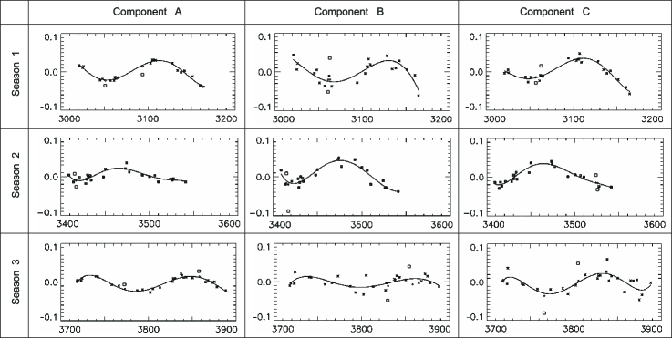
Figure 6: Light curves of the A, B and C components of PG1115+080 from observations in 2004, 2005 and 2006 (seasons 1-3), and their approximations by series expansions in Legendre polynomials up to the 5-th order without the zero and first-order terms. The ”bad” points (see Sec. 2) are shown by squares.

5 Quadruple lens PG 1115+080

The quadruply lensed quasar PG1115+080 is among the systems, which need more accurate estimates of the time delays. This is the second gravitational lens system, for which the time delays have been measured (Schechter et al. 1997). Soon after the first measurements, revision of the same data with another algorithm was published (Barkana 1997), which in general confirmed the results by Schechter et al. (1997). New determinations of the time delays from observations of 2004-2006 at the Maidanak Observatory were reported in 2009 (Vakulik et al.). The next attempt to reanalyse the data by Schechter et al. was made by Eulaers & Magain (2011) with the use of two methods. All the known time delay estimates for PG 1115+080 are collected in Table 5.

The data presented in Table 5 explain our desire to reprocess the data by Vakulik et al.(2009) with the use of our new algorithm. Indeed, while the time delay estimates for pairs BA and AC deviate from each other in different authors rather randomly, the estimates of $\Delta t_{BC}$ in Vakulik et al. (2009) and Eulaers & Magain (2011) are definitely lower than those presented by Schechter (1997) and Barkana (1997). Note, in particular, a good agreement between $\Delta t_{BC}$=17.9 days obtained by Eulaers & Magain (2011) with the Minimum Dispersion method, and $\Delta t_{BC}$=16.4 days in Vakulik et al. (2009).

In Fig. 6, three light curves for three seasons are shown together with the corresponding approximations by series expansions in the normalized Legendre polynomials. Because of the smallness of the time delays between A1 and A2 predicted by the macrolens model from the system geometry, their light curves were joined to form a single A light curve.

Similar to the light curves of HE 0435-1223 in Fig. 3, the terms of the zeroth and first orders are omitted in displaying in Fig. 6. Qualitatively, the mutual time shifts are visible by sight in all seasons, namely, the B component leads A and C quite evidently. Concerning the A-C pair one can say only that the expected time delay value is rather small. The least scatter of the data points with respect to the approximating polynomial is observed for the A component, and the largest one is for B, that is quite natural since the latter is the faintest one.

The largest time delay value, $\Delta t_{BC}$, which equals 23.7 days in Schechter et al. (1997) and 25.0 days in Barkana (1997), was estimated by Eulaers & Magain (2011) to equal 20.8 days in reprocessing the same data with the NMF (Numerical Model Fit) method, and 17.9 days with the MD (Minimum Dispersion) method. The latter value is consistent both with that obtained from the 2004-2006 data by Vakulik et al. (2009) – 16.4 days, and with the results of reprocessing in the present work – 16.8 days.

The time delay values for the two other image pairs are consistent in different works much worse. In this respect, compare a scatter of the time delay values from Table 5 with the indicated estimates of errors. We see $\Delta t_{CA}$ varying from 7.5 to 12 days in different authors, with the error estimates from 0.9 to 3.9 days; $\Delta t_{BC}$ ranges between 16.4 and 25 days, with the errors varying between 3.4 and 6.9 days; and finally, $\Delta t_{BA}$ varies from 4.4 to 14.3 days, while the errors are from 2.0 to 3.4 days. As is seen, the values of delays vary in a wider range than it follows from the estimates of their error bars. This fact should not in effect wonder: investigators know that estimates of the time delays may be sensitive to the patterns of random fluctuations of sampling points, which are often indistinguishable from the actual signal features. This concerns especially the sparse and scanty data, that is just the case for the PG 1115+080 data, both by Schechter et al. (1997) and Vakulik et al. (2009). The results of averaging the estimates of differential delays obtained in this work from different seasons are shown in the last line of Table 5, and the results for only the first season are shown in the last but one line.

It is evident that the time delays in the PG 1115+080 system need to be further specified, but it is evident also that no essential progress can be expected from processing the available data. Long-term monitoring with a sufficient sampling rate is needed, which would provide new high-quality photometric data.

6 Discussion and conclusions

Summarizing, we would like to note the following.

• The proposed method implies a pair-wise comparison of light curves represented by their polynomial approximations. In this respect, our algorithm is similar to the regression difference technique illustrated by Tewes et al. (2013) in calculations of the time delays in HE 0435-1223.

• We tested the method for robustness and bias using the mock light curves issued for the TDC0 campaign (Liao Kai et al. 2015). The method demonstrates resistance to exclusion of up to 33% of light curve data points and shows no noticeable change in the relative deviations from the true delay values $A_{j}$ exceeding 0.04. The testing has also shown that in 6 cases of 30 successful determinations the value of $A_{j}$ is less than 0.01.

• The estimates of the time delays in the quadruply lensed quasars PG 1115+080 and HE 0435-1223 obtained with the method proposed in this work are consistent with those obtained for these objects with other methods earlier. As is shown in Sec. 3, the short time delays are measured with the worst relative precision (see Table 1). In PG 1115+080 and HE 0435-1223, we deal with just this case.

• The differences of our approach from those proposed by other authors earlier do not have a fundamental nature, but provide convenience in calculations. In particular, our approach allows to exclude or add some of the approximating polynomial terms without a necessity to recalculate the coefficients. This provides a simple way to mitigate the effects of microlensing for the case of ”slow” microlensing events. The method can be useful for a preliminary express analysis of the data flow expected from the future sky survey programs.

References

- Barkana (1997) Barkana R., 1997, ApJ, 489, 21
- Bonvin (2016) Bonvin V., Tewes M., Courbin F., Kuntzer T., D. Sluse D., G. Meylan G., 2016, A&A, 585,
- Burud (2000) Burud I. et al., 2000, ApJ, 544, 117
- Courbin (2011) Courbin F. et al., 2011, A&A, 536, A53
- Cuevas-Tello (2006) Cuevas-Tello C., Tino P., Raychaudhury S., 2006, A&A, 454, 695
- Dobler (2013) Dobler G., Fassnacht C., Treu T., Marshall P.J., Liao K., Hojjati A., Linder E., Rumbaugh N., 2015, ApJ,799, 168
- Eulae11 (2011) Eulaers E., Magain P., 2011, A&A, 536, A44
- Eulae13 (2013) Eulaers E. et al., 2013, A&A, 553, A121
- Falco85 (1985) Falco E.E., Gorenstein M.V., Shapiro I.I., 1985, ApJ Letters, 289, L1
- Flor84 (1984) Florentin-Nielsen R., 1984, A&A, 138, L19
- Hojjati (2013) Hojjati A., Linder E.V., 2014, PhRvD, 90, 123501
- KochSchech (2004) Kochanek C., Schechter P., 2004, Measuring and Modeling the Universe, from the Carnegie Observatories Centennial Symposia. Published by Cambridge University Press, as part of the Carnegie Observatories Astrophysics Series. Edited by W. L. Freedman, p. 117.
- Kochan (2006) Kochanek C., Morgan N., Falco E., McLeod B., Winn J., Dembicky J., Ketzeback B., 2006, ApJ, 640, 47
- Korn (2000) Korn G.A, Korn T.M., 2000, Mathematical Handbook for Scientists and Engineers: Definitions, Theorems, and Formulas for Reference and Review. Dover Publications, Inc., Mineola, N.Y.
- Kund (1997) Kundič T. et al., 1997, ApJ, 482, 75
- Lehar (1992) Lehar J., Hewitt J., Burke B., Roberts D., 1992, ApJ, 384, 453
- liao (2015) Liao K. et al., 2015, ApJ, 800, 11
- Morgan (2008) Morgan C., Eyler M.E., Kochanek C.S., Morgan N.D., Falco E.E., Vuissoz C., Courbin F., Meylan G., 2008, ApJ, 676, 80
- Pelt (1994) Pelt J., Hoff W., Kayser R., Refsdal S., Schramm T., 1994, A&A, 286, 775
- Pelt (1996) Pelt J., Kayser R., Refsdal S., Schramm T., 1996, A&A, 305, 97
- Press (1992) Press G., Rybicki G., and Hewitt J., 1992, ApJ, 385, 404
- Rathna (2013) Rathna Kumar S., et al., 2013, A&A, 557, A44
- Refsdal (1992) Refsdal S., 1964, MNRAS, 128, 307
- Schechter (1997) Schechter P.L. et al., 1997, ApJ, 475, L85
- Sch_Chol (1986) Schild R.E., Cholfin B., 1986, ApJ, 300, 209
- sch_thom (1997) Schild R.E., Thompson D.J., 1997, AJ, 113, 130
- Tewes (2012) Tewes M. et al., 2012, Msngr, 150, 49
- Tewes (2013a) Tewes M., Courbin F., Meylan G., 2013, A&A, 553, A120
- Tewes (2013b) Tewes M., et al., 2013, A&A, 556, 10 pp
- Vakulik (2009) Vakulik V.G. et al., 2009, MNRAS, 400, L90
- sch97 (1997) Vanderriest C., Schneider J., Herpe G., Chevreton M., Moles M., Wlerick G., 1989, A&A, 215, 1
- Xu (2015) Xu D., Sluse D., Schneider P., Springel V., Vogelsberger M., Nelson D., Hernquist L., 2015, MNRAS, 456, 739
- Walsh (1979) Walsh D., Carswell R.F., Weymann R.J., 1979, Nature, 279, 381