High Performance Rearrangement and Multiplication Routines for Sparse Tensor Arithmetic

Abstract

Researchers from diverse disciplines are increasingly incorporating numeric high-order data, i.e., numeric tensors, within their practice. Just like the matrix-vector (MV) paradigm, the development of multi-purpose, but high-performance, sparse data structures and algorithms for arithmetic calculations, e.g., those found in Einstein-like notation, is crucial for the continued adoption of tensors. We use the motivating example of high-order differential operators to illustrate this need. As sparse tensor arithmetic represents an emerging research topic, with challenges distinct from the MV paradigm, many aspects require further articulation and development. This work focuses on three core facets. First, aligning with prominent voices in the field, we emphasise the importance of data structures able to accommodate the operational complexity of tensor arithmetic. However, we describe a linearised coordinate (LCO) data structure that provides faster and more memory-efficient sorting performance in support of this operational complexity. Second, flexible data structures, like the LCO, rely heavily on sorts and permutations. We introduce an innovative permutation algorithm, based on radix sort, that is tailored to rearrange already-sorted sparse data, producing significant performance gains. Third, we introduce a novel poly-algorithm for sparse tensor products, where hyper-sparsity is a possibility. Different manifestations of hyper-sparsity demand their own customised approach, which our multiplication poly-algorithm is the first to provide. These developments are incorporated within our LibNT and NTToolbox software libraries. Benchmarks, frequently drawn from the high-order differential operators example, demonstrate the practical impact of our routines, with speed-ups of $40\%$ or higher compared to alternative high-performance implementations. Comparisons against the MATLAB Tensor Toolbox show over $10$ times speed improvements. Thus, these advancements produce significant practical improvements for sparse tensor arithmetic.

siscxxxxxxxx–x

1 Introduction

Efficient sparse-matrix data structures and algorithms have had an unquestionably massive impact on the field of technical computing. In recent years, however, algebra and calculations for high-order data, which we call numeric tensors [30], have begun to enjoy a prominent role. We use the “numeric” adjective to differentiate this research topic from geometric tensors. The latter must meet strict mathematical or physical properties, whereas this is not necessarily the case for all uses of numeric high-order data. Thus, for the remainder of this work, we use “tensor” to mean the numeric variant.

In fact, the need for mature sparse computations may be even more acute in the tensor domain than in the MV domain. If using a dense representation, the computational and memory demands of working with tensors grows exponentially with order, raising barriers to tractability. For this reason, circumventing “the curse of dimensionality” that harries tensor operations is a crucial goal. Apart from work into low-parametric representations [7, 45, 44, 34] and implicit representations of high-order operators [1, 2, 17], researchers have also focused on how to explicitly represent sparse tensors [14, 39, 38, 4, 26, 5, 32, 47].

Tensor decomposition drives a great deal of this work [14, 39, 38, 4, 5, 32], but applications involving high-order linear operators [1, 2, 17, 47], high-order partial derivatives [26], and deep learning [20] also see need for sparse tensors. Additionally, the known link between symmetric tensors and polynomial equations [15] introduces further impetus for sparse tensor computations. Considering the high-sparsity of real-world polynomial equations [53], if tensors are used to manipulate such equations, efficient sparse algorithms will be needed (likely along with symmetric-specific optimizations [50]).

As Bader and Kolda [3, 4] and we [30] have argued, a suite of core tensor data structures and algorithms can allow fast prototyping and development of algorithms applied to high-order data. A further argument can be made that multi-purpose algorithms and data structures for tensor arithmetic operations, i.e., those found in Einstein-like notation [30, 31, 1, 2], are a valuable tool for working with and understanding tensor operations [30, 1, 2]. These include multiplication, solution of linear equations, and addition/subtraction. Combined with an interface that supports Einstein-like notation, core tensor arithmetic computations would be an important part of a technical computing framework for tensors, analogous to the environments used for MV algebra and computations, e.g., MATLAB. We note that core arithmetic routines would not obviate the need for specialised data structures and algorithms, e.g., those used for the ubiquitous alternating least-squares (ALS) algorithm [36].

The topic of data structures and algorithms for multi-purpose sparse tensor arithmetic has been broached previously by Bader and Kolda [4] as part of their MATLAB Tensor Toolbox (MTT). Yet, since the MTT does not provide high-performance kernels of its own [50], there is considerable opportunity for continued investigation. With this vision in mind, this work offers a set of core kernels for sparse tensor arithmetic. Sharing Bader and Kolda’s [4] design philosophy of not favouring any particular index over another, this work describes a LCO sparse-tensor data structure, which is related to, but different from, the one seen in the MTT. The flexibility and simplicity of the LCO data structure comes at the cost of heavily relying on sorts and permutes. This work describes high-performance rearrangement algorithms specifically tailored for sparse tensors. Finally, this paper describes a multiplication poly-algorithm that can effectively compute the products between any tensors exhibiting any manner of sparsity, including hyper-sparsity.

Detailed benchmarks demonstrate the high performance of these algorithms. To provide a motivating example, many of the benchmarks are drawn from the exemplar of using Einstein-like notation to construct high-order differential operators. Because the impact of different data-structure and algorithmic choices are just beginning to be understood within sparse tensor arithmetic, we limit our focus to sequential implementations. This also makes any performance comparisons with the MTT more fair, whose sparse tensor arithmetic functionality is predominantly based on sequential algorithms within MATLAB. All computations are implemented within our open-source LibNT and NTToolbox software libraries, whose dense tensor routines have been previously introduced as part of the NT framework [30].

§2 begins by using the example of high-order differential operators, applied to images, to motivate the development of high-performance routines to support the tensor arithmetic operations found in Einstein-like notation. With these preliminaries discussed, §3 outlines a flexible data representation for sparse tensors. This data representation places a heavy burden on fast methods to rearrange data, which §4 addresses by outlining algorithms to permute sparse tensors. Sparse-tensor multiplication is discussed in §5. Comparative performance with the MTT, and a high-performance re-implementation of its multiplication strategy, is highlighted in §6. Finally §7 discusses and concludes this work. Tests were performed on a Windows $64$-bit workstation, using an Intel E8400 CPU with 8 Gb of memory. All algorithms are implemented as part of LibNT’s C++ code, to which the MATLAB library NTToolbox interfaces.

2 High-Order Differential Operators

Many scientific domains require software tools to work with and algebraically manipulate high-order numeric data [30]. High-order differential operators are one such important exemplar [1, 2]. We make this more concrete by focusing on high-order operators applied in computer vision using an Einstein-like notation, but we emphasise that the need for sparse tensor arithmetic transcends both computer vision and high-order differential operators.

Applied to gridded data, e.g., an image, often representing a partial differential equation, differential operators commonly take the form of finite-difference (FD) operators. Such operators may be explicitly needed within optimization problems, e.g., where the operand of the differential operator is an unknown that must be solved using a least squares method. For length $N$ first-order data, sparse FD matrix operators are relatively easy to construct. For example, should $O(h^{2})$ central differencing be required, the sparse FD matrix can be constructed with MV algebra using

(10) $$\textbf{D}=\dfrac{1}{2}\left\{\left(\begin{array}[]{ccc}\textbf{0}&0&0\\ -\textbf{I}&\textbf{0}&\textbf{0}\\ \textbf{0}&0&0\\ \end{array}\right)+\left(\begin{array}[]{ccc}0&0&\textbf{0}\\ \textbf{0}&\textbf{0}&\textbf{I}\\ 0&0&\textbf{0}\\ \end{array}\right)+\left(\begin{array}[]{ccccccc}-3&4&-1&\textbf{0}&0&0&0\\ \textbf{0}&\textbf{0}&\textbf{0}&\textbf{0}&\textbf{0}&\textbf{0}&\textbf{0}\\ 0&0&0&\textbf{0}&-1&4&-3\\ \end{array}\right)\right\}\textrm{,}$$

where the first and last rows of D are filled using $O(h^{2})$ forward and backward-differencing operators. Each term in (10) is an $N\times N$ matrix, meaning $\mathbf{I}$ is of size $(N-2)\times(N-2)$. The 0 sub-matrices are sized based on this and whether they share a row or column with $\mathbf{I}$ or a scalar. Unfortunately, working with FD operators of higher order using MV algebra and software can be prohibitively challenging and error prone, as users must work with “flattened” versions of the operators and operands [1, 2]. The challenges only multiply as order increases, e.g., 3D medical imaging scans, or a time series of such scans. Thus, it can be beneficial to express and programmatically construct such operators within their natural high-order domain [1, 2].

When dealing with generative models used in computer vision, often FD operators across different image indices are incorporated. One of many examples is depth-map and albedo estimation [28], illustrated by Figure 1.

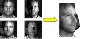
Fig. 1: Illustration of depth-map & albedo estimation. Four images of a single-view image sequence are displayed. Each image corresponds to a distinct principal light direction, with its own shading characteristics. From the image sequence, an estimate of the depth of the subject’s face, along with the albedo, can be produced through a combinatorial Laplacian formulation. Although not discussed here, anisotropic elements, using entry-wise products, are frequently required to manage image noise [28]. Image data obtained from the Extended Yale Face Database B [24].

Estimating the phenomenon in question requires constructing a design tensor and inverting a sparse system of high-order linear equations. Using Einstein-like notation [30, 31, 1, 2], and assuming a 2D image domain, such systems can be expressed in general terms as

(11) $$y_{ij}=a_{ijk\ell}x_{k\ell}\textrm{,}$$

where repeated and non-repeated indices denote inner and outer products, respectively, $x_{k\ell}$ is the tensor of quantities of interest, e.g., a depth-map, $y_{ij}$ are observations relevant to the generative model, and $a_{ijk\ell}$ is a sparse design tensor. A common makeup of the design tensor is the combinatorial Laplacian:

(12) $$a_{ijk\ell}=d^{(y)}_{ii^{\prime}}\delta_{j\ell}d^{(y)}_{i^{\prime}k}+d^{(x)}_{jj^{\prime}}\delta_{ik}d^{(x)}_{j^{\prime}\ell}\textrm{,}$$

where $d^{(.)}_{ij}$ is the sparse tensor version of the FD matrix of (10) and $\delta_{ij}$ is the Kronecker delta. Frequently, the Laplacian operator is also anisotropic, e.g., to manage image noise [28], and nonlinear formulations can also be required [29, 27]. Representing such complexities benefits further from Einstein-like notation, but for the sake of simplicity we limit the exposition to the isotropic and linear example of (12).

Equipped with an appropriate computational environment, a researcher or practitioner could programmatically construct $a_{ijk\ell}$ using an Einstein-like notation. For example, LibNT and/or NTToolbox [30] will execute (12) as binary operations left-to-right with operator precedence. As we will elaborate, the executed products include hyper-sparse matrix products, requiring a strategy different from those found in standard sparse matrix multiplication. In addition, the multiplication, addition, and assignment operations will require rearrangements of non-zero values. Thus, there is a demand here for sparse tensor rearrangement and multiplication algorithms. We will return to these equations to provide an application-based context for this work’s contributions.

3 Data Representation

This section first outlines considerations for sparse tensor representation, highlighting the LCO format used in LibNT. Afterwards, some comparative results demonstrate the LCO format’s effectiveness.

3.1 Concepts

Sparse MV computations rely on compressed formats [18, 11], e.g., the compressed sparse-column (CSC) format, which allows efficient column-centred operations at the expense of inefficient row-centred operations. However, Bader and Kolda [4] convincingly argue against compressed tensor formats, as it requires categorising an index, or set of indices, differently from others, which becomes less meaningful as the tensor order increases.

These arguments are bolstered by considering tensor arithmetic’s operational complexity, i.e., the enormous number of ways that tensor indices can match up differently for the same arithmetic operation. For instance, enumerating all possible inner/outer product possibilities between two $N$-order tensors requires calculating all partial permutations of the $N$ indices. Partial permutations [6] are calculated using,

(13) $$P=\sum_{i=0}^{N}i!{N\choose i}^{2}\,\textrm{,}$$

which grows factorially with order. Similar conclusions are drawn when considering the index matchings within Einstein-like notation for addition and subtraction, as the number of possible index matchings also increases factorially with order.

This operational complexity suggests that data structures for sparse tensor arithmetic should be as flexible as possible. While several authors have adapted the compressed approach for non-arithmetic purposes [14, 39, 38, 26], these solutions would struggle to accommodate arithmetic operational complexity. Compression schemes would need to be re-computed or there would have to be different code implementations depending on what tasks are performed on what indices. Such strategies become less viable for tensor arithmetic with each increase in order.

Bader and Kolda make the case for a concurrent list of non-zero data and index values. When an operation demands a different lexicographical order a rearrangement, i.e., a sort or permute, is required. Thus, no indices are favoured over others in terms of operational efficiency, but rearrangements then play a heavy role. This approach has also been used within computational chemistry [47] and deep learning [20].

The coordinate (CO) and LCO sparse formats are the two main non-compressed choices that store their non-zeros using straightforward lists. The CO format stores expanded index values, i.e., for an $N$-order tensor each of the $N$ index values. In contrast, the LCO format stores linearised index values, i.e., $N$ index values represented by a single integer value. For instance, the zero-based LIVs for a third-order tensor, $a_{ijk}$, can be calculated using

(14) $$\mathit{LIV}=i+n_{i}(j+n_{j}k)\textrm{,}$$

where $n_{(.)}$ denotes the range of the corresponding index. Such a lexicographical order places greatest significance on the third index, followed by the second and first indices, which we designate numerically as $\{0,1,2\}$. Any permutation of the $\{0,1,2\}$ sequence is also valid, and this scheme is trivially extended to higher orders. Table 1 illustrates the differences between the two formats. Of note is that the sparse formats are identical for first-order tensors.

Table 1: The CO and LCO sparse formats. Example zero-based index values from a $4\times 4\times 4$ sparse tensor, with a lexicographical order of $\{0,1,2\}$, illustrate the two formats.

CO Index Values:	$\{1,0,0\}$	$\{2,0,1\}$	$\{0,1,1\}$	$\{3,2,2\}$	$\{1,0,3\}$	$\{2,2,3\}$
LCO Index Values:	$1$	$18$	$20$	$43$	$49$	$58$

Both formats rely on a lexicographical order to arrange non-zero values. For the CO format, $\{0,1,2\}$ indicates that when comparing values, the third index value must be considered first, followed by the second and first index values. Altering the lexicographical order requires changing the sequence in which expanded index values are compared. In contrast, for the LCO format, the lexicographical order governs the linearisation scheme used to compute LIVs. Changing the lexicographical order necessitates recomputing LIVs, which we call LIV shuffle. Once done, a straightforward integer comparison then suffices to compare LIVs.

Bader and Kolda opt for the CO sparse format for the MTT library [4]. While Bader and Kolda do not specifically discuss the LCO format, they do mention concerns with linearisation schemes in general, arguing that LIVs may overflow integer datatypes. This is a valid concern. However, many applications, such as computer vision [27], computational chemistry [47], and deep learning [20], often employ tensors whose dimensionalities fit within a 64-bit limit (or 63-bit limit if using signed integers). For cases where LIVs do exceed standard integer limits, e.g., problems involving the SNAP dataset [41], high-precision integer libraries [40, 25] could offer very-large LIVs. Nonetheless, here we limit our scope to tensors whose dimensionality fits within the signed integer limits of $2^{63}-1$, leaving the topic of very-large LIVs to future work.

Moving on from overflow issues, other factors also play an important role. For instance, compared to the CO format and assuming all index values are stored using the same fixed-sized integer datatype, the LCO format is more memory efficient for tensor orders greater than one. With additional bookkeeping, less memory could be used in the CO format by employing variable-sized integers, e.g., choosing 8-bit, 16-bit, 32-bit, or 64-bit integers for each index based on its dimension. However, such extra bookkeeping and complexity comes with its own penalties. Moreover, developing an efficient implementation using high-performance statically-typed languages, without using costly dynamic polymorphistic operations, is not easily resolved. As a result, the exploration of variable-sized CO indices is left for future work.

With the above caveats in mind, there is an increased cost of certain fundamental operations when using the CO format. For instance, comparison operations in the CO format require up to $N$ individual numerical comparisons for an $N$-order tensor. Such comparison operations are fundamental kernels within sorting algorithms and arithmetic operations built on the format. Additionally, the increased memory requirements degrade locality between consecutive non-zero index values, resulting in more cache misses, which can be the deciding factor in sorting performance [37]. This also impacts arithmetic operations. These considerations all add up to the CO format placing greater demands on memory bandwidth, which is often the limiting factor in modern computer architectures [21].

On the other hand, the LCO format requires an LIV shuffle to change lexicographical orders. Thus, putting memory storage requirements aside, choosing between the two can come down to comparing the impact of the increased comparison, read, and write CO costs vs. the $O(\mathit{nnz})$ LIV shuffle step of the LCO format. Benchmark tests can measure the relative impact of these costs.

3.2 Benchmarks

As the example in §2 highlights, rearrangements of non-zero data is a frequent requirement for tensor arithmetic. For instance, to perform the addition in (12), one of the terms must be re-sorted based on the index matching. We call rearranging already sorted data into a new lexicographical order permutation, which can benefit from specialised algorithms that we discuss in more detail in §4. However, for the sake of simplicity, here we focus on sorting algorithms to compare the two formats. Sorting is typically required when non-zero data is unsorted, e.g., after tensor construction or the insertion of un-ordered non-zeros. We first discuss details on the data formats we test, followed by an explanation of the sorting algorithms used in the benchmarks. Afterwards we highlight the results of two different tests.

Two variants of the CO format were tested. The first, denoted CO_Separate and used within the MTT, uses contiguous memory regions to store specific expanded index values, e.g., the first coordinates are stored contiguously, followed by the second, and so on. We also tested a second variant that packs expanded index values consecutively one after each other, thereby better maximising memory locality across consecutive accesses of tensor elements. We call this variant CO_Packed. If the $N$ index values of each of the $M$ non-zeros were stored in an $M\times N$ matrix, CO_Separate and CO_Packed would arrange them in column- and row-major order, respectively.

As changing the lexicographical order is often performed prior to rearranging data, we also measure the LIV shuffle cost for the LCO format. If executed naively, this operation can be very expensive as LIV shuffles require integer division. However, we use a fast division library [19] to mitigate this cost.

For the most part, experiments are restricted to using signed $64$-bit integers to store index values. Nonetheless, we do briefly explore the use of fixed $16$-bit signed integers for the CO format to help shed light on any performance impacts of using smaller-sized integers.

Tests employed two well-known sorting algorithms. The first corresponds to the introspective sorting algorithm [43], used in the C++ standard and considered a gold-standard [42]. The second corresponds to most-significant digit (MSD) radix sort [52], which, unlike general sorting algorithms, is designed specifically for integer-like data. Experiments used C++ implementations, adapted from optimised and publicly available general-purpose versions [51, 23] to handle the CO_Separate, CO_Packed, and the LCO formats, along with the accompanying data array. Attesting to their speed, we found that in our tests our CO_Separate implementation always outperformed MATLAB’s sortrows, which is the approach the MTT uses to sort its CO_Separate data. Code can be found within our publicly available LibNT library. More details on our implementations can be found in our supplemental material.

The first test measured times to sort a fifth-order sparse tensor. As mentioned, we also recorded the time needed to shuffle LIV values. As integer division operations are extraordinarily fast when divisors are a power of two, index ranges were chosen to be $2^{10}-1$ to avoid providing the LCO format with an unfair advantage. To judge the impact of tensor order, the same tensor was also “flattened” into lower-order LCO and CO formats. Thus the impact of increasing tensor order, with its increased demands on memory bandwidth and LIV shuffles, was measured under identical conditions.

Figures 2(a) and (b) outline the results of this first test, using introspective and MSD radix sort, respectively.

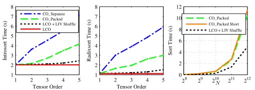
(a)

(b)

(c)

Fig. 2: Sorting times of the LCO, CO_Packed and CO_Separate sparse formats. (a) and (b) depict the time to sort a fifth-order $N\times N\times N\times N\times N$ tensor, with $N=2^{10}-1$ and $5N^{2}$ non-zeros, using the introspective and MSD radix sort algorithms, respectively. The time taken with flattened lesser-order versions and with shuffling LIVs was also measured. (c) depicts the MSD radix sort run time of CO_Packed Short, a $16$-bit variant of CO_Packed, and LCO plus an LIV shuffle to perform the sort needed to add the fourth-order tensors in (12).

As the figures demonstrate, shuffling LIVs comes with a non-trivial running-time cost, which increases with order. However, the cost of sorting both variants of the CO format is greater, meaning that even with an LIV shuffle included, sorting LCO indices is still much faster than sorting second-order or higher CO indices.

To contextualise these results within the differential operators application, we also measured sorting times to add the two fourth-order tensor terms in (12) using the best performing algorithm of MSD radix sort applied to the LCO and CO_Packed formats. These terms are formed after the necessary products are executed, and can be denoted $c_{ij\ell k}^{(y)}$ and $c_{jik\ell}^{(x)}$, where the ordering of indices post-multiplication follows LibNT’s conventions [27]. We assume both tensors lie in the $\{0,1,2,3\}$ lexicographical order, meaning to perform the addition one of the tensors must be re-sorted into the $\{1,0,3,2\}$ lexicographical order. While this is technically a permutation task, measuring differences in using general-purpose sorting algorithms can still be informative to assess data-format performances. We assume input images are of size $N\times N$, making each tensor size $N\times N\times N\times N$, and we measure sorting times for increasing values of $N$. Figure 2(c) depicts a plot of the sorting times, demonstrating the large gain in speed of the LCO format. In particular, at the highest value of $N$, the LCO format plus the LIV shuffle consumes $4.9\,s$, whereas CO_Packed consumes $10.4\,s$.

For the highest $N$, once the tensors are sorted the run time for the addition operation is only $2.7\,s$ for the LCO format. Thus, sorting the LCO format takes roughly $65\%$ of the total operation time. In contrast, for the CO format, should the addition operation consume roughly the same amount of time, sorting would consume $80\%$ of the total time, demonstrating both the importance of optimising rearrangements and the importance of data format choice for sparse tensor arithmetic.

To shed light on the prospect of using variable-sized integers, we also tested the sorting performance of CO_Packed when using fixed $16$ bit integers to hold each coordinate. While this scheme does not address how to best implement a variable-sized approach, it does help reveal if using smaller-sized integers may allow CO_Packed to outperform LCO. However, as Figure 2(c) demonstrates, the $16$-bit variant of CO_Packed consistently ran slightly slower than the $64$-bit variant. One possible explanation for this is that $64$-bit architectures, like the one used for testing, may be better optimised to operate in its native bit size. While this question does deserve further investigation, these preliminary tests further support the conclusion that LCO enables faster sorting speed regardless of the underlying CO datatype.

In sum, these results indicate that the LCO format is better able to manage the demands of increasing tensor orders. This is crucial when operating with sparse tensors of high orders, such as those seen in computational chemistry [47, 33], computer vision [27] or deep learning [20]. Considerable performance differences were also evident at lower orders. Coupled with the fact that the LCO format uses much less memory at high orders when using native bit sizes, these performance metrics lead us to prefer the LCO sparse format over either CO format variant.

4 Permutation

As noted, a non-compressed sparse format places a heavy demand on rearranging non-zero data. Consequently, fast and efficient sparse tensor arithmetic can hinge on the algorithmic choices made for rearrangements. For sorting, this was demonstrated by Figure 2(a) vs (b), where MSD radix sort performed roughly twice as fast as introsort. For this reason, we opt for MSD radix sort as the sorting algorithm for sparse tensors. Our supplemental material includes more extensive experiments supporting this conclusion, comparing MSD radix sort against three other leading algorithms.

Yet, permutation, i.e., rearranging already sorted data into a different lexicographical order, is arguably even more important than sorting. In the MV paradigm such tasks are called transposition. Because of operational complexity, tensors are frequently arranged in an undesired lexicographical order, making sparse permutation a frequent first step within tensor arithmetic. In fact, this was already demonstrated in the benchmarks of Figure 2(c), where a permutation was required to perform the sum in (12). While permutation operations are tasked with the same goal as sorting, i.e., rearranging data into a desired lexicographical order, their starting points differ. By taking advantage of the existing structure of already sorted non-zero data, faster means to permutation can be realised. These speedups can be quantified using benchmarks.

4.1 Algorithm

When permuting data the first step is to recompute the LIVs into the new lexicographical order. The work needed for the subsequent rearrangement depends on the relationship between the starting and ending lexicographical orders. For instance, intuitively it should be simpler to permute sparse tensor data from the $\{0,1,2,3\}$ lexicographical order to the $\{1,0,2,3\}$ lexicographical order than it would be to permute it to the $\{3,2,1,0\}$ lexicographical order. The former only rearranges two indices, while the latter rearranges all of them. This intuition stems from the fact that regardless of their starting and ending lexicographical orders, new LIVs will always be arranged in sequences of sorted sublists. Specific subsequences of these sublists must be merged together, creating new sequences of sorted lists that may be in the right arrangement or may require additional merges. This relationship can be formalised, providing for a ready identification of efficiencies.

A permutation essentially divides tensor indices into two sets—those that require rearranging and those that do not. Figure 3 illustrates how this can be determined, with a third-order tensor $a_{ijk}$.

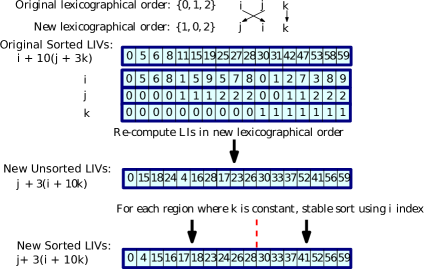
Fig. 3: Permuting a $10\times 3\times 2$ third-order tensor, $a_{ijk}$. The figure depicts the original and new LIVs corresponding to starting and ending lexicographical orders of $\{0,1,2\}$ and $\{1,0,2\}$, respectively. The index of highest significance in the new LIVs is a resting index, so regions where $k$ is constant can be sorted independently. Each such independent region must be stably sorted based on the rearrangement index $i$. The final resting index $j$ can be ignored. Note that the $i$, $j$, and $k$ indices are rendered for the sake of illustration, but in the radix permutation (RP) algorithm indices are computed on-the-fly using integer division and modulo operations.

The top of the figure illustrates the bipartite graph of the starting and ending arrangements of $i$,$j$,$k$. Because the $i$ index crosses an index that originally had a higher significance, i.e., $j$, the new LIVs must be rearranged according to the $i$ index. We call such indices rearrangement indices. The other two indices do not meet this criterion and thus, the new LIVs do not need to be rearranged according to $j$ and $k$. These indices we call resting indices.

Categorising the indices this way breaks the permutation task into a recursive hierarchy of steps. For instance, working from highest-to-lowest significance of the new LIVs in Figure 3’s example, $k$ is a resting index. As a result, regions where $k$ is constant can each be independently sorted. These independent regions can be stably sorted based solely on the $i$ index, which is a rearrangement index. Stability means the original relative ordering is used to break ties between equal values. The next resting index $j$ is also the final index, so there is no more work to do. However, if $j$ was not the final index, then the process would have to continue, where each sub-region where $j$ is constant would be sorted. This process can be generalised to arbitrary orders and starting/ending lexicographical orders. An important aspect to note is that the final index is always a resting index.

Returning to Figure 3’s example, identifying regions in the new LIVs where $k$ is constant can be done by integer dividing the starting LIV by $n_{j}n_{i}=30$ to compute the $k$ value, and then computing the maximum possible LIV at that value of $k$. A linear scan that stops when this threshold is broken identifies the end-point of the region. The process can be repeated for the next value of $k$. Separating the LIV values into independent parts benefits all sorting algorithms. For comparison sorts, the asymptotic bounds may be lowered. However, for radix sorts, within each region of constant $k$, each LIV can be examined modulo $30$, reducing the maximum possible integer magnitude to accommodate. Depending on the radix digit size, this can reduce the key length, thereby reducing the number of passes a radix sort need perform. Moreover, when sorting each independent region of constant $k$, the LIVs modulo $30$ need only be stably sorted using the rearrangement index $i$. Thus each LIV modulo $30$ can be reduced even further by integer dividing by $n_{j}=3$. In the general case, this aggressive shaving off of irrelevant portions of the LIVs can drastically reduce the key length for radix sorts, significantly reducing the number of passes the sort must perform.

To take advantage of these characteristics, LibNT includes an algorithm, called RP. Given a starting and ending lexicographical order, a preprocessing step determines which indices are rearrangement or resting indices. The RP routine then employs a stable, but not inplace, variant of the MSD radix sort algorithm. Since shaving off irrelevant portions of the LIVs relies on integer division, libdivide [19] is used to to minimise slowdowns. Nonetheless, even when using a fast integer-division library, shaving off LIVs comes with a computational cost, which can only be justified if the number of radix sort passes can be reduced. This is typically the case when both the number of non-zeros (NNZ) and reductions in LIV magnitude are large. For this reason, LibNT’s RP algorithm is adaptive and will switch to the standard MSD radix sort based on an estimate of the reduction in pass numbers.

There are theoretically interesting implications of permuting sparse tensor data this way. As Sedgewick explains, radix sorts are often sublinear in the information content of the keys being sorted [52], meaning they can often arrange data without examining every bit. However, this is only an average-case result based on random conditions. Yet, in the context of sparse-tensor permutations, by always having at least one index a resting index, it is always possible to permute without examining every bit in the LIVs. Whether these theoretical gains translate to practical ones is a matter revealed by benchmarks.

4.2 Results

Tests measured the permutation performance of RP using all $4!-1=23$ permutations of a fourth-order tensor. Figure 4(a) first depicts differences in run time between RP and the MSD radix sort algorithm (negative values are better for RP) to permute the fourth-order combinatorial Laplacian tensor in (12). This operator’s fill factor decreases quadratically with dimensionality, which produces highly-sparse fill factors at large dimensionalities. Figure 4(b), on the other hand, depicts results of a fourth tensor whose fill factor remains a constant $2\%$. Both sets of tests were performed at increasing levels of dimensionality. While other algorithms were also tested, including those well suited to sorting already sorted sublists, e.g., natural mergesort, only the MSD radix sort algorithm proved competitive to RP.

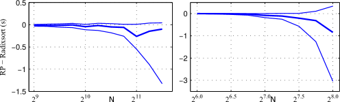
(a)

(b)

Fig. 4: Permutation benchmark results. (a) and (b) depict the differences in time between RP and radixsort to permute $N\times N\times N\times N$ tensors. Positive and negative values mean RP ran slower and faster, respectively. (a) and (b) use the combinatorial Laplacian in (12) and a tensor with $2\%$ fill factor, respectively. All $23$ possible permutations were performed, with the heavy-weighted line displaying median run time differences across all permutations, and lighter-weighted lines depicting maximum and minimum differences.

As the graph demonstrates, when examining the median run time across all permutations, RP typically performed slightly better than MSD radix sort, indicating that most permutations provide an opportunity for further optimization. More importantly, certain permutations provide even greater speed-up opportunities, with the RP algorithm running at significantly faster speeds. To shed some more light on this, Table 2 depicts timings corresponding to those of Figure 4(a) at $N=2^{11.5}$.

Table 2: Permutations and run times of RP vs. MSD radix sort, corresponding to the maximum, median, and minimum differences in time. All timings drawn from Figure 4(a) at $N=2^{11.5}$.

Ranking	Permutation	MSD Radix Sort (s)	RP (s)
Max	$\{3,1,2,0\}$	3.50	3.54
Median	$\{2,1,3,0\}$	3.54	3.45
Min	$\{1,0,2,3\}$	2.71	1.38

As can be seen, a permutation like $\{1,0,2,3\}$, which only requires that RP rearrange according to the second index, allows a roughly $50\%$ increase in speed.

These results demonstrate that when opportunity affords, RP can significantly speed up permutations. Considering that the MSD radix sort already represents one of the fastest means to sort LCO data, these improvements attest to the value of using specialised permutation algorithms. It is expected that these gains would only increase with higher orders and greater NNZs.

5 Multiplication

Multiplying two sparse tensors together epitomises the unique demands of sparse tensor arithmetic. Any tensor multiplication, involving inner, entrywise, and outer products, can be represented as a sequence of matrix products [30]. Thus, sparse matrix products play a fundamental role in executing sparse tensor products. However, as §5.1 will explain, hyper-sparsity comes into play, calling for different strategies than those found in the MV paradigm. Answering this need, §5.2 outlines an effective multiplication poly-algorithm designed to handle operands exhibiting any manner of hyper-sparsity.

5.1 Hyper-Sparsity

Sparse tensors often exhibit hyper-sparsity. Typically raised in an MV context, hyper-sparsity refers to matrices where the numbers of rows and columns exceed the NNZ [8, 9]. Applied to a tensor context, this meaning implies a dimension that exceeds the NNZ. While comparatively rare in linear algebra, graph algorithm applications, which see uses for tensors [22], encounter hyper-sparsity frequently [8, 9].

However, even when tensors are not hyper-sparse on their own, they can exhibit hyper-sparsity when they are mapped to matrices during multiplication. For instance, as Figure 5(a) demonstrates, flattening a purely diagonal tensor

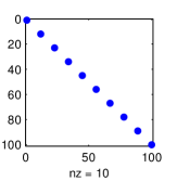
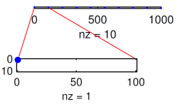
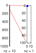
(a)	(b)	(c)

Fig. 5: Hyper-sparsity of a matricised tensor. A fourth-order diagonal tensor $a_{ijk\ell}$, meaning all-zero except for when $i=j=k=\ell$, can produce hyper-sparse matrices when flattened: (a) depicts the hyper-sparsity pattern when a $10\times 10\times 10\times 10$ diagonal tensor is matricised so that two of its indices are mapped to rows while the remaining are mapped to columns. An example multiplication causing this would be $a_{ijk\ell}a_{k\ell mn}$. (b) depicts the same tensor, except that it is matricised by mapping one index to rows, while the remaining are mapped to columns; (c) depicts the same as (b) except that the role of rows and columns are reversed. In the example multiplication of $a_{ijk\ell}a_{jk\ell m}$ the first and second operands would exhibit the patterns in (b) and (c), respectively. The two figures of (b) and (c) depict column- and row-sparsity, respectively, while (a) depicts index-sparsity.

can produce index-sparse matrices, meaning both row and column ranges exceed the NNZ. In addition, as Figure 5(b) and (c) demonstrate, flattening operations can also produce row- and column-sparse matrices, often manifesting as very-tall and very-wide matrices, respectively, in which only one of the dimensions exceeds the NNZ. Such a case occurs in the differential operators example of §2, which we return to in §6. Thus, any routine executing sparse tensor products must be able to handle hyper-sparsity.

5.2 Poly-Algorithm

Sparse-tensor multiplication can be executed in three steps:

1. map sparse-tensor LCO data to a matrix, using a permute or sort if needed;

2. convert each LCO matrix to an appropriate multiplication datatype (MDT), e.g., CSC, and multiply;

3. map the resulting matrix back to a sparse tensor.

This is similar to the scheme used by the MTT. However, the MTT always uses the CSC MDT and algorithm. However, the standard CSC and compressed sparse-row (CSR) MDTs are not equipped to handle hyper-sparsity [8, 9]. This explains why the MTT excises all-zero columns and rows before performing standard CSC multiplication, requiring that each matrix be sorted twice and also necessitating additional bookkeeping which incurs its own running-time and memory costs. The reader is encouraged to consult our supplementary material for a more detailed explanation of the sorting and bookkeeping costs associated with excising all-zero rows and columns. In our experience, mirrored by others [47] and in the tests of §3.2, sorting or permuting costs can be a major run time cost in sparse tensor computations. For this reason, we minimise them as much as possible.

Thus, an attractive alternative is to employ algorithms and MDTs specialised to naturally handle the different types of hyper-sparsity that can possibly be encountered. Choosing different MDTs is not a freedom typically enjoyed within the MV paradigm, in which matrices, once constructed, are typically locked into a single datatype and lexicographical order. Yet, this is not an issue in a sparse tensor context, where a conversion to an MDT is required regardless. This extra flexibility calls for a poly-algorithm that dispatches to specific multiplication algorithms and MDTs depending on whether the flattened tensors are sparse, row-sparse, column-sparse, or index-sparse.

Table 3

Table 3: Multiplication possibilities based on sparse characteristics of operands. Table entries indicate the algorithm LibNT employs, along with the section number describing it, for each sparse-characteristic combination.

	Sparse	Row-Sparse	Column-Sparse	Index-Sparse
Sparse	CSC/CSR
(§5.2.2)	CSC
(§5.2.2)	CSC
(§5.2.2)	CSC
(§5.2.2)
Column-Sparse	CSR
(§5.2.2)	DCSC/DCSR
(§5.2.3)	DCSC
(§5.2.3)	DCSC
(§5.2.3)
Row-Sparse	CSR
(§5.2.2)	DCSR
(§5.2.3)	CSCNA/ CSRNA
(§5.2.4)	CSCNA
(§5.2.4)
Index-Sparse	CSR
(§5.2.2)	DCSR
(§5.2.3)	CSRNA
(§5.2.4)	SOP
(§5.2.5)

outlines the $16$ different possible sparsity combinations. In addition, it details the algorithmic choices used by LibNT. Two considerations motivated these choices. The primary consideration was on ensuring memory use and run time were not dependant on any hyper-sparse dimension sizes. As Buluç and Gilbert [8, 9] warn, algorithms, e.g., the CSC, whose run time and memory use depend on the dimensionalities of the matrix can consume inordinate amounts of memory or exhibit impractical run times under hyper-sparse conditions. With the first consideration satisfied, the second goal was gaining the fastest run time and/or the lowest memory use. Unlike MV computations, performance metrics of sparse-tensor multiplication must include the cost of converting to the MDT.

In describing the different multiplication algorithms, this subsection will use a set of common notation outlined in Table 4. While entrywise products are an important concept in tensor computations, their presence only means that the tensor product is mapped to a repeated sequence of matrix products [30], which does not change the basic approach of sparse-tensor multiplication. Thus, for simplicity only inner/outer products will be considered, explaining why the first and second operands of Table 4 are single matrices.

Table 4: Multiplication Notation

First Operand	$\mathbf{A}$	Second Operand	$\mathbf{B}$
Rows and Columns of $\mathbf{A}$	$m$ and $k$	Rows and Columns of $\mathbf{B}$	$k$ and $n$
Number of Columns of $\mathbf{A}$ with one or more non-zeros	$\mathit{nzc}_{\mathbf{A}}$	Number of Rows of $\mathbf{B}$ with one or more non-zeros	$\mathit{nzr}_{\mathbf{B}}$
Number of Rows of $\mathbf{A}$ with one or more non-zeros	$\mathit{nzr}_{\mathbf{A}}$	Number of Columns of $\mathbf{B}$ with one or more non-zeros	$\mathit{nzc}_{\mathbf{B}}$

Apart from the notation of Table 4, this section will use $f$ to refer to the number of floating-point operations in a multiplication, which is the same for all algorithms. $\mathbf{C}$ will denote the matrix product of $\mathbf{A}$ and $\mathbf{B}$. To make the exposition simpler, the subsection will focus mostly on column-by-column versions of the algorithms, e.g., CSC. As such, $f(i)$ will denote the number of floating-point operations to compute the $i$th column of $\mathbf{C}$ and $\mathit{nnz}_{\mathbf{C}}(i)$ will denote the resulting NNZ. LibNT tests for hyper-sparsity by measuring the ratio of NNZ to the dimension in question. For example, the row-sparsity of $\mathbf{A}$ can be tested by measuring whether $m/\mathit{nnz}_{A}>1$.

To begin the discussion, §5.2.1 outlines the dataset used for benchmarking. Afterwards, §5.2.2 focuses on LibNT’s implementation of the standard sparse multiplication algorithm. This is followed by §5.2.3 and §5.2.4 which describe specialised algorithms to multiply a column-sparse with a row-sparse matrix and a row-sparse with a column-sparse matrix, respectively. Finally, §5.2.5 describes LibNT’s algorithm to multiply two index-sparse matrices.

5.2.1 Dataset

Datasets used for testing can consist of real-world examples or synthetic datasets, which are parameterised and/or randomly generated. While real-world datasets do exist, e.g., those used in decomposition techniques applied to networks [35, 46], these datasets do not consist of many examples. Thus, to characterise sparse-multiplication algorithms under different conditions, e.g., NNZs, hyper-sparsities, and dimension sizes, this work uses a synthetic dataset. Nevertheless, we return to the differential operators example in §6 to provide comparative benchmarks in an application-based context.

We use a third-order tensor generalisation of the R-MAT recursive graph model [13], which can control for dimension size, fill factor, and fill pattern. In the original R-MAT model, the recursive base edge probabilities are specified for each quadrant. To generalise to a third-order R-TENSOR, the BEP must be specified for each octant. Table 5

Table 5: Base edge probabilities used for the R-TENSOR model in the sparse multiplication experiments with their octant specified in parentheses. To add variability into experiment runs, the probabilities were adjusted by additive values drawn from a uniform distribution of $[-.1\,\,.1]$ and renormalised so that they all sum to $1$.

Octant:	$(1,1,1)$	$(1,1,2)$	$(1,2,1)$	$(1,2,2)$	$(2,1,1)$	$(2,1,2)$	$(2,2,1)$	$(2,2,2)$
BEP:	$.3$	$.5/6$	$.5/6$	$.5/6$	$.5/6$	$.5/6$	$.5/6$	$.2$

outlines the probabilities used for this work. The symbols $a_{ijk}$ and $b_{ijk}$ will be used to denote R-TENSORs. R-TENSORs can manifest column-, row-, or index-sparsity depending on their fill factor and how they are flattened. Maximum NNZs were limited by what our workstation could handle when using the CSC/CSR formats at the highest levels of hyper-sparsity. This allows us to demonstrate the benefits of specialised hyper-sparse formats even when settings allow the use of standard formats.

5.2.2 Standard CSC/CSR

The tried-and-tested column-by-column CSC algorithm relies on a dense, size $k$, singly-compressed array to quickly access columns and a dense, size $m$, accumulator array to quickly collect non-zeros as each column of $\mathbf{C}$ is constructed. Readers unfamiliar with these algorithms and requisite index and accumulator arrays are encouraged to consult Davis [18] and Buluç et al. [11]. Table 6

Table 6: Characteristics of the three different column-by-column multiplication algorithms. Importantly, run times include the cost to convert to the MDT from column-major LCO data. Memory use only includes temporary data structures used for multiplication.

Algorithm	Sparse Accumulator	Column Indexing	Run time	Memory Use
CSC	yes	singly-compressed	$\mathcal{O}(m+k+\mathit{nnz}_{\mathbf{A}}+\mathit{nnz}_{\mathbf{B}}+f+\sum_{i}^{n}\mathit{nnz}_{\mathbf{C}}(i)\log\mathit{nnz}_{\mathbf{C}}(i))$	$\mathcal{O}(m+k)$
DCSC	yes	doubly-compressed	$\mathcal{O}(m+\mathit{nnz}_{\mathbf{A}}+\mathit{nnz}_{\mathbf{B}}+f+\sum_{i}^{n}\mathit{nnz}_{\mathbf{C}}(i)\log\mathit{nnz}_{\mathbf{C}}(i))$	$\mathcal{O}(m+\mathit{nzc}_{\mathbf{A}})$
CSCNA	no	singly-compressed	$\mathcal{O}(k+\mathit{nnz}_{\mathbf{A}}+\mathit{nnz}_{\mathbf{B}}+\sum_{i}^{n}f(i)\log f(i))$	$\mathcal{O}(\max f(i)+k)$

summarises the salient characteristics of the CSC algorithm.

When both matrices present no hyper-sparsity, LibNT opts for the CSC or CSR algorithms. LibNT gains additional efficiency by converting only one of the matrices to compressed form. For instance, the CSC algorithm only requires fast access of the columns of $\mathbf{A}$, meaning it suffices if $\mathbf{B}$ is simply stored in column-major LCO format. The primary consideration to choose between the two algorithms is based on what minimises any extra sorts. For instance, if the lexicographic order of both tensors happened to produce column-major matrices once they were flattened, then the CSC algorithm will be chosen. In cases were both flattened matrices must be rearranged, the choice is based on a simple heuristic of run time costs of the CSC and CSR algorithms. Run time between the two is almost identical, except for the final summation term, where the CSR algorithm must sort each row of $\mathbf{C}$ instead of each column. Assuming somewhat uniform distribution of non-zeros across rows and columns, the run time for the sort should be smaller if the task is broken into a greater number of pieces. Thus, LibNT opts for the CSC format when $n>m$, otherwise it chooses CSR.

Finally, by avoiding converting one of the matrices to compressed form, the applicability of the standard algorithms can be extended to greater numbers of cases. For instance, as long as $\mathbf{A}$ has no hyper-sparsity, the standard CSC algorithm can be applied, regardless whether $\mathbf{B}$ is row-, column-, or index-sparse. Thus, the CSC and CSR algorithms can be employed beyond the sparse-sparse case, explaining the first column and row of Table 3.

5.2.3 DCSC/DCSR

Hyper-sparsity challenges the CSC/CSR algorithms in two manners. The first corresponds to cases where using singly-compressed arrays for row or column access are no longer tenable. For instance, should two cubic R-TENSORS be multiplied using

(15) $$a_{ijk}b_{\ell jk}\textrm{,}$$

the left and right operands would be mapped to very-wide and very-tall matrices, respectively. Consequently, when $N^{2}\gg\mathit{nnz}$ using the CSC or CSR datatypes is prohibitive or even intractable.

A solution is offered by Buluç and Gilbert [8], who introduced the doubly compressed-sparse column (DCSC) and doubly compressed-sparse row (DCSR) formats, which remove run time and memory-use dependance on $k$. Thus, their column-by-column multiplication algorithm can be executed when $\mathbf{A}$ is column-sparse. Similarly, the DCSR algorithm can handle cases when $\mathbf{B}$ exhibits row sparsity. Even when $k$ still fits comfortably within memory, the doubly-compressed scheme can produce highly significant speedups. Both variants come at the cost of additional memory accesses, compared to the standard CSC and CSR options, and so they are not used when the level of hyper-sparsity is likely insufficient to reap the benefits.

To demonstrate these points, experiments used the CSC and DCSC algorithms to compute (15). The tests used cubic R-TENSORs generated with NNZs ranging from $4e5$ to $1e6$ in increments of $1e5$. Column-sparsity of the R-TENSORs ranged from $1$, i.e., no column-sparsity, to $500$, i.e., $1$ non-zero per $500$ columns, in log10-scale increments. The NNZ and column-sparsity govern the corresponding dimensions of the R-TENSOR. This was performed $3$ times for each NNZ/column-sparsity combination. Finally, two different types of runs were performed. The first run used two different R-TENSORs in (15) and the second used the same R-TENSOR for each operand.

Differences in run time were primarily dependent on the hyper-sparsity, and not dimensionality. The relative run times across different levels of hyper-sparsity are depicted in Figure 6(a). As the figure demonstrates,

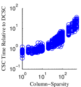
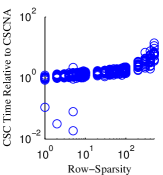
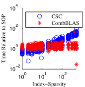
(a)	(b)	(c)

Fig. 6: Run times of the multiplication algorithms under differing levels and types of hyper-sparsity. (a) graphs the ratio of running-times of the CSC vs. the DCSC algorithm under different levels of column-sparsity, while (b) measures the ratio of the CSC vs. the CSCNA algorithms under different levels of row-sparsity. (c) graphs the ratio of the CSC and CombBLAS algorithms to LibNT’s SOP algorithm under different levels of index-sparsity. For all scenarios, performance ratios correlated the most with hyper-sparsity levels.

a column-sparsity value of $10$ separates the point at which the DCSC algorithm outperforms CSC. As column-sparsity increases, the DCSC algorithm’s run time is on average roughly $20$ times faster than the CSC approach, demonstrating a tremendous amount of speedup.

For the purposes of LibNT’s poly-algorithm, the library opts for the DCSC algorithm whenever column sparsity exceeds $3$. While lower than the threshold indicated by Figure 6(a), this satisfies the primary consideration of keeping memory use proportional to the NNZs. LibNT uses the same criteria explained in §5.2.2 to choose between the DCSC and DCSR variants. As well, and indicated in Table 3, LibNT uses the DCSC algorithm whenever $\mathbf{A}$ is column-sparse and for all cases of $\mathbf{B}$, except when the latter presents no hyper-sparsity. The reverse holds true for the DCSR algorithm.

5.2.4 CSCNA/CSRNA

§5.2.3 outlined a multiplication strategy to handle cases when using the dense CSC and CSR access arrays becomes untenable. In the opposite scenario, i.e., multiplying a very-tall matrix with a very-wide one, the dense access arrays of the CSC and CSR data structures pose no problems and it is the accumulator array that can become untenable. For example, this situation would manifest should two R-TENSORs be multiplied using

(16) $$a_{ijk}b_{\ell mk}\textrm{.}$$

In this situation, the standard CSC and CSR algorithms can be modified to forego the accumulator array, resulting in the compressed sparse-column no-accumulator (CSCNA) and compressed sparse-row no-accumulator (CSRNA) algorithms, respectively. In the column-by-column case, jettisoning the accumulator array means that as each column of $\mathbf{A}$ is constructed the non-zeros are not collected and summed together in one step. Instead for each column $i$, $f(i)$ values are computed and stored in a simple LCO list. These $f(i)$ values must then be sorted and any data values with the same LIV are then summed together. As Table 6 indicates, this results in an increased sorting burden, but comes at the benefit of not having memory use and run time be dependent on the potentially huge number of rows of $\mathbf{A}$. Note that in this scenario, it is possible to also perform an inner-product algorithm [11]. However, due to excessive run times, discussed in more detail in our supplemental material, we do not include its results in our graphs.

As with the DCSC algorithm, improvements can be garnered even when the very-large dimensions fit comfortably in memory. To test this, the R-TENSOR experiments in §5.2.3 were repeated, except that (16) was computed. NNZs ranged from $1e5$ to $3e5$ in increments of $5e4$. Apart from this change, all other test settings were kept identical. Figure 6(b) depicts the results of this test, graphing the ratio of run times of the CSC algorithm to the CSCNA algorithm under different levels of row-sparsity. As the figure demonstrates, apart from some outliers at low-levels of row-sparsity, the CSCNA algorithm is able to match or exceed the CSC algorithm. At row-sparsity values of roughly $3$ or higher the CSCNA algorithm begins to exhibit faster execution speeds than the CSC algorithm, eventually running on average $6$ times faster. Nonetheless, in isolated instances the CSCNA algorithm performed considerably worse. Characterising when these situations occur is an important area for further investigation. Even so, as the CSCNA algorithm posts excellent performance for the far majority of trials and avoids having memory use and run time depend on $m$, LibNT opts for the CSCNA approach whenever row-sparsity is greater than $3$.

As before, LibNT uses the same criteria explained in §5.2.2 to choose between the CSCNA and CSRNA variants. LibNT also opts for the CSCNA algorithm whenever $\mathbf{A}$ is row-sparse and $\mathbf{B}$ is index-sparse while the CSRNA is chosen when $\mathbf{B}$ is column-sparse and $\mathbf{A}$ is index-sparse.

5.2.5 SOP

The final case to consider is when both $\mathbf{A}$ and $\mathbf{B}$ are index-sparse. Buluç and Gilbert [8, 9] have demonstrated that the outer-product approach is fast and memory efficient for this scenario. Under this approach, $\mathbf{A}$ and $\mathbf{B}$ must be sorted in different lexicographical orders—column- and row-major, respectively. As the top of Figure 7 demonstrates,

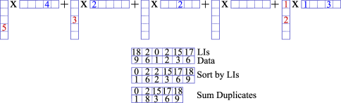
Fig. 7: The outer-product multiplication algorithm. Using example matrices, the top of the figure demonstrates how the outer-product algorithm would multiply each column of $\mathbf{A}$ with each row of $\mathbf{B}$. Below, the SOP algorithm used by LibNT to sum each of the $k$ rank-$1$ matrices is illustrated.

each column of $\mathbf{A}$ is multiplied with each row of $\mathbf{B}$, producing $k$ $m\times n$ rank-$1$ matrices. To produce the final result, these rank-$1$ matrices must be summed together. Under an index-sparse setting, both $\mathit{nzc}_{\mathbf{A}}$ and $\mathit{nzr}_{\mathbf{B}}$ are each less than $k$, and not all non-zero columns of $\mathbf{A}$ have a matching non-zero row of $\mathbf{B}$. Thus, the number of rank-$1$ matrices to sum together is always less than $k$ and often less than $\min(\mathit{nzc}_{\mathbf{A}},\mathit{nzr}_{\mathbf{B}})$.

As part of their CombBLAS library, Buluç and Gilbert use their DCSC and DCSR formats in combination with a heap-like data structure to merge the rank-$1$ matrices [9]. Buluç and Gilbert’s motivating problem is large-scale parallel matrix multiplication. As such, the authors correctly did not account for the time to construct doubly-compressed matrices in their performance metrics, because their parallel algorithm amortises these costs across sub-tasks. In contrast, the conversion costs to the MDT must be considered in a sparse-tensor setting.

As a result, approaches with minimal conversion costs should also be considered. As the bottom of Figure 7 illustrates, one approach, which we call the simple outer-product (SOP) algorithm, is to just directly concatenate all the intermediate rank-$1$ matrices together into a length $f$ LCO data-structure. This LCO array can then be sorted based on the LIVs, with duplicate entries being summed together. The downside is the $\mathcal{O}(f)$ memory use and a $\mathcal{O}(f\log{}f)$ sort, which dominates the complexity. However, unlike in regular sparse settings, $f$ can often be small compared to the NNZ of $\mathbf{A}$ and $\mathbf{B}$. Moreover, the ratio of $f$ to the NNZ of $\mathbf{C}$ can also be close to $1$, meaning strategies to efficiently add duplicate entries do not always justify their overhead.

These conclusions are borne out when multiplying R-TENSORs using a very similar setup as the experiments in §5.2.3. However, instead of cubic R-TENSORs, $M\times N\times N$ tensors are used instead, where $M=N^{2}$. Thus, when flattening the R-TENSORs to compute (15), the resulting matrices exhibit square dimension sizes of $N^{2}\times N^{2}$, providing appropriate conditions to vary the row- and column-sparsity together. Additionally, the NNZs varied from $5e4$ to $1e5$ in increments of $1e4$ and the time taken for the CSC, SOP, and CombBLAS’ [10] C++ index-sparse algorithm, including setup costs, was measured. All other conditions were kept the same.

The results of this test are depicted in Figure 6(c). The SOP algorithm outperformed the CSC algorithm at most of the index-sparsity range. Inspection of the numerical results reveal that faster run times begin at index-sparsities greater than $6$, with the performance gap increasing to roughly $35$ times faster execution at the highest levels of index-sparsity. Compared to the CombBLAS algorithm, the SOP outperformed it on average by a factor of $2$ at all levels of index-sparsity, demonstrating the value of a simplified approach in sparse tensor settings. However, in several instances CombBLAS outperformed the SOP algorithm, indicating that certain scenarios call for a more sophisticated merging approach. Further work should focus on identifying these scenarios a priori. Even so, the SOP executed the fastest on almost all test instances.

As a result, LibNT opts for the SOP algorithm whenever both $\mathbf{A}$ and $\mathbf{B}$ are index-sparse. For the purposes of satisfying the primary consideration of avoiding highly excessive memory use, the SOP algorithm is applied whenever both row- and column-sparsity exceed $3$.

6 Comparative Performance

So far, this work has contrasted performance of different algorithmic choices. What has not been discussed is the impact of using such high-performance kernels in an actual multi-purpose sparse-tensor arithmetic setting. Returning to the differential operators example of §2 and using left-to-right precedence, the first term in (12) can be broken into two binary products, with the second written as

(17) $$b^{(y)}_{ii^{\prime}j\ell}d^{(y)}_{i^{\prime}k}\textrm{,}$$

where $b^{(y)}_{ii^{\prime}j\ell}=d^{(y)}_{ii^{\prime}}\delta_{j\ell}$. Assuming uniform index ranges, when flattened (17) describes an $N^{3}\times N$ row-sparse matrix as the left operand multiplied with a standard sparse $N\times N$ matrix.

To unearth some of the significance of using this work’s techniques, we compare the performance of NTToolbox against two alternatives in executing (17). The first alternative is the MTT. Like the NTToolbox, the MTT relies on a MATLAB frontend to setup and call optimised compiled-language backends, except that the former uses LibNT’s C++ algorithms specialised for tensor arithmetic, while the latter relies on MATLAB’s optimised, but general-purpose, built-in routines. Differences in performance will be partly driven by any limitations that the MATLAB environment imposes upon the MTT. The MTT handles all hyper-sparsity combinations by executing CSC multiplication after excision of all-zero rows and columns. As such, the number of sorts performed remains constant, i.e., through MTT’s three and two calls to MATLAB’s unique function and CSC sparse matrix construction routines, respectively. A head-on comparison helps uncover when NTToolbox’s specialised high-performance kernels are warranted over the convenience of a pure MATLAB implementation.

The second alternative is an NTToolbox re-implementation of the MTT’s multiplication strategy, using a LibNT-based backend. For fair comparison, care was taken in optimising this approach, e.g., only converting the right operand to the CSC MDT and avoiding the superfluous excision of all-zero columns of the right operand. Thus, differences in performance will be driven solely by the impact of the poly-algorithm vs. the all-purpose strategy of CSC multiplication combined with excision used in the MTT.

Tests assumed input images of size $N\times N$, where $N=2^{k}-1$, with increasing values of $k$. The subtraction of $1$ ensures the integer division libraries used by NTToolbox are not given an unfair advantage. The time needed to rearrange both operands into the required lexicographical order for the poly-algorithm was included in the measurements. Figure 8(a) graphs the run times of all three implementations,

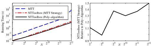
Fig. 8: Comparative performance of NTToolbox multiplication poly-algorithm vs. the MTT and an NTToolbox implementation of the MTT’s multiplication strategy. All graphs depict the run time to execute the hyper-sparse products in (12). (a) graphs all three run times in logarithmic scale, whereas (b) graphs the run time of the NTToolbox (MTT strategy) vs. the NTToolbox (poly-algorithm).

demonstrating that NTToolbox speeds up the calculation by an order of magnitude or more. Figure 8(b) depicts the run time of the NTToolbox (MTT strategy) relative to the NTToolbox (poly-algorithm), demonstrating that the latter speeds up computations by $40\%$ or more at high dimensionalities. For context when $N=2^{11}-1$ the run time of the MTT, NTToolbox (MTT strategy), and NTToolbox (poly-algorithm) were $23.7\,s$, $2.7\,s$, and $2.0\,s$, respectively. For the NTToolbox-specific tests, the performance improvements of the poly-algorithm can mainly be attributed to eliminating superfluous permutations, meaning only those required to flatten operands into matrix form are executed.

7 Conclusion

LibNT offers a multi-purpose environment for the sparse tensor arithmetic operations seen in Einstein-like notation, meaning addition, subtraction and multiplication, and the solution of equations incorporating dense, sparse, or dense/spase tensor mixtures. This work focused on three core aspects. First, like Bader and Kolda [4], we believe a multi-purpose arithmetic library should not place an a priori precedence on certain tensor indices over others. However, we argue for the LCO format over Bader and Kolda’s CO format, presenting results showing faster sort run times. Importantly, these benefits come with a smaller memory footprint, especially at higher orders. Currently tensor dimensionalities are limited to $63$ bits, but future work incorporating very-large integer datatypes should remove this limitation, extending the LCO’s benefits to a greater set of tensor problems.

Secondly, we emphasise the importance of high-performance rearrangement algorithms when using list-like data structures such as the CO and LCO formats. Such algorithms are necessary to realise a high-performance sparse tensor arithmetic library. This work outlined the impact of using radix sort, which is specialised to sort integer datatypes, over more general-purpose sorting algorithms. Importantly, we also outline how to take advantage of the inherent structure of sparse data to speed up the frequent permutations required for list-like data structures. An algorithm exploiting these underlying characteristics was developed, outperforming the fastest standard sorting option and demonstrating the value of employing specialised approaches to sparse tensor arithmetic.

Finally, we addressed how to implement sparse-times-sparse tensor multiplication, an operation that exemplifies the unique requirements of sparse tensor arithmetic. A multi-purpose library could encounter any combination of sparse, index-sparse, column-sparse, or row-sparse data, which all demand their own specialised approaches. Apart from highlighting this unique characteristic, we also outlined a multiplication poly-algorithm that can choose appropriate algorithms accordingly. The poly-algorithm ensures that excessive memory use is avoided, a potentially catastrophic event. Moreover, the poly-algorithm produces highly-significant reductions in run time over the common CSC/CSR approach. While the MTT can also handle hyper-sparsity, its one-size-fits-all algorithm does not exploit the very distinct features of the different sparsity types.

We demonstrate the impact of this work on several benchmarks derived from the application of high-order differential operators. These tests are complemented by other benchmarks incorporating randomly generated sparse tensors. Compared to the MTT, the outlined kernels contributed to considerable improvements in run time on constructing high-order combinatorial Laplacians, demonstrating the value of this work’s specialised and high-performance kernels. The discussed high-performance kernels are accessible through the LibNT and NTToolbox, which are open-source libraries for Einstein-like notation, implemented in C++ and MATLAB, respectively. However, the data structures and algorithms described here, or variants thereof, are also well suited to any other package incorporating sparse tensor arithmetic.

Considerable future work can further advance the state of sparse-tensor arithmetic. In particular, multi-core and heterogeneous routines would be welcome, e.g., parallel approaches to radix sort [49]. Another possibility is to leverage work within the graph algorithm community on parallel sparse matrix-matrix multiplication [9, 12]. Efficiencies stemming from symmetry of sparse tensors, possibly adapting existing dense approaches [50], should also be incorporated. Reducing temporary memory allocation in chained arithmetic expressions should help reduce overhead. Finally, adapting LibNT to be able to handle very-large integers as LIVs is highly important. These and other advancements will help further the impact of this, and other [4, 47], efforts towards establishing a mature body of sparse tensor arithmetic routines.

8 Supplemental Material

8.1 Sorting

We provide more details on the performance of MSD radix sort vs competitor algorithms in sorting sparse tensor data. When sorting LIVs, another array, i.e., the data array, must be sorted alongside it. By increasing the memory bandwidth needed to perform rearrangements, cache misses can be more predominant, which is often the leading factor in sorting performance [37]. The LCO sorting task can be categorised as sorting with “satellite” data [16], which is often tackled using pointers to the additional data or by using data structures containing key/record pairs. In contrast, sorting LCO data requires sorting a contiguous integer-valued LIV array with a contiguous and separate data array acting as satellite data. The importance of fast sorting speed to the sparse LCO format makes it highly worthwhile to focus on optimising sorts.

We tested and adapted several different algorithms using our own C++ implementations. The leading comparison-based sorting algorithms that were tested include the highly prominent introspective sort [43], adapted from Schwarz [51], and Timsort [48]. Integer sorting algorithms were also tested, including a least-significant digit (LSD) radix sort [52] and an in-place version of MSD radix sort [23] that uses no extra memory. All of the tested algorithms were adapted to sort the LCO data array alongside any movements of the LCO LIV array. In addition, effort was taken to optimise their implementations, including using hybrid and adaptive approaches, in order to achieve fast run times.

Two different types of tests were performed. The first type of test, depicted in Figure 9(a),

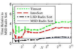
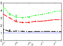
(a)	(b)

Fig. 9: Benchmark results of different sorting algorithms applied to sparse fourth-order tensors. (a) and (b) depict results from randomly generated $N\times N\times N\times N$ sparse tensors, with a fill factor of a fourth-order Laplacian and a $5\%$ fill factor, respectively. Tests were run on increasing values of $N$ and repeated $10$ times. Trend lines represent median values and error bars represent quartiles.

measures the sorting time on a randomly-generated tensor matching the fill-factor of a fourth-order Laplacian operator, e.g., one that can act on an image. The Laplacian operator’s fill factor decreases quadratically with dimensionality, providing a highly-sparse test setting. While it is important to measure performance in a highly-sparse setting, it is also worthwhile to test under settings where sparsity does not vary quadratically with dimensionality. Along those lines, Figure 9(b) depicts sorting times of fourth-order tensors with $5\%$ fill factors.

As the figure makes clear, both radix sorts beat out the two comparison sorts in a highly-sparse setting, posting $2$ to $4$ times faster speeds for most of the range of dimensionalities. These results are more striking when considering that the benchmark setup is directly unfavourable to radix sorts. More specifically, a fourth-order Laplacian’s fill factor decreases quadratically, meaning the maximum size of the LIV increases at a quadratic rate compared to the linear rate increase of the NNZ. This can be problematic for radix sorts, because its run time is proportional to the magnitude of the keys being sorted [52], i.e., the LIVs. Nonetheless, these results indicate that radix sort can perform extremely well even in this demanding setting. One likely reason for this is that both radix sort variants used a commonly recommended [52] hybrid implementation that switched to a comparison-based sort when appropriate. Thus, dependence on the magnitude of the LIVs is relaxed.

Similar results were produced when the algorithms were tested on sparse tensors with $5\%$ fill factor, with the radix sorts outperforming their comparison counterparts by highly significant margins.

Apart from illustrating the high-performance of radix sorts, these results demonstrate the significant impact of algorithm choice in sorting sparse tensors. Depending on the choice of algorithm, sorting can take roughly $2$-$4$ times longer, which is of high consequence when considering the importance of rearrangement operations to sparse tensor computations. In terms of whether the LSD or MSD variant is preferable, the latter generally outperformed the former, particularly at very-large values of $N$. Moreover, the MSD version used here is inplace. For these reasons, LibNT uses MSD radix sort.

8.2 Excising All-zero Rows and Columns

We provide more details on the rationale for why we avoid excising all-zero rows and columns and use instead specialised algorithms designed to handle hyper-sparsity. To help make our explanation as concrete as possible, we use an example where two tensors have been flattened into matrices, $\mathbf{A}$ and $\mathbf{B}$, to execute a tensor product. These are multiplied together in the equation $\mathbf{A}*\mathbf{B}$. First, we will assume $\mathbf{A}$ is row-sparse and proceed through the four possible hyper-sparsity options of $\mathbf{B}$. Second we will assume $\mathbf{B}$ is row-sparse and proceed through the four possible hyper-sparsity options of $\mathbf{A}$

Before beginning with the first case, i.e., assuming $\mathbf{A}$ is row-sparse, we note that one approach to handle $\mathbf{A}$’s row-sparsity, regardless of the hyper-sparsity of $\mathbf{B}$, is to sort $\mathbf{A}$ in row-major order, excise the all-zero rows, and then re-sort $\mathbf{A}$ back in column-major order. $\mathbf{B}$ would be sorted once into column-major order. In this scenario, CSC multiplication can be executed, which can be done by only converting the excised version of $\mathbf{A}$ into the CSC format and leaving $\mathbf{B}$ in LCO format, which avoids any possible issues should $\mathbf{B}$ be hyper-sparse in any way. This approach, however, requires an extra sort, which is why we avoid this option.

Going through the four possible hyper-sparsity characteristics of $\mathbf{B}$ brings up the following considerations:

1. $\mathbf{B}$ is simply sparse. In this case, we can sort both matrices in row-major order, excise all-zero rows of $\mathbf{A}$, and then perform standard CSR multiplication. However, in CSR multiplication, only $\mathbf{B}$ need be in compressed form. So in this scenario, only $\mathbf{B}$ need be converted to CSR form, and $\mathbf{A}$ can be kept in row-major LCO form. This approach requires no excisions.

2. $\mathbf{B}$ is row-sparse. The number of columns of $\mathbf{A}$ must match the number of rows of $\mathbf{B}$ to be a valid matrix multiplication. As a result, even though $\mathbf{B}$ is row-sparse, because $\mathbf{A}$ is not column-sparse, we know that we can safely store the CSR version of $\mathbf{B}$. Thus, there is no need perform any excision, and the standard CSR algorithm can be employed, keeping $\mathbf{A}$ in row-major LCO form.

3. $\mathbf{B}$ is column-sparse. There are several options in this case:

   1. To stay with the excision approach we can sort both matrices in row-major order and then perform standard CSR multiplication. However, because $\mathbf{B}$ is column-sparse, the sparse accumulator used in the CSR algorithm can consume amounts of memory far exceeding the NNZ of either $\mathbf{A}$ or $\mathbf{B}$. Thus, to perform the CSR algorithm, $\mathbf{B}$ would need to be first sorted in column-major order, have its all-zero columns excised, and then be re-sorted in row-major order. Similar issues apply if we attempt to perform CSC multiplication. Thus, an additional expensive sort would be required.

   2. Another option is to sort $\mathbf{A}$ and $\mathbf{B}$ in row- and column-major orders respectively and perform an inner product algorithm [11], which does not require excising all-zero rows and columns. A sparse accumulator can be used to store one-by-one either the non-zero rows of $\mathbf{A}$ or the non-zero columns of $\mathbf{B}$. However, in this case, the run time cost would be either $\mathcal{O}(\mathit{nzr}_{\mathbf{A}}\mathit{nnz}_{\mathbf{B}})$ or $\mathcal{O}(\mathit{nzc}_{\mathbf{B}}\mathit{nnz}_{\mathbf{A}})$, which is typically on the same order of magnitude as $\mathcal{O}(\mathit{nnz}_{\mathbf{A}}\mathit{nnz}_{\mathbf{B}})$. In our experiments, this option ran one to three orders of magnitude slower than the CSCNA or CSRNA algorithms. For this reason, we do not include its results in this work.

   3. Due to the above considerations, we use a variant of the CSC and CSR algorithms, CSCNA and CSRNA, respectively, that eschew the sparse accumulator, thus avoiding the need for additional re-sorts or the use of the expensive inner-product algorithm. The choice of CSCNA vs. CSRNA is based on the criteria given in Section 4.2.3. Either way no excisions are required.

4. $\mathbf{B}$ is index-sparse. Similar issues as the previous case ensue, except with even more complications. However, since $\mathbf{A}$ is only row-sparse, we can use the CSCNA algorithm and data structure.

To help complete this picture, we also outline the issues that arise if $\mathbf{B}$ is row-sparse and proceed through the following four hyper-sparsity options of $\mathbf{A}$:

1. $\mathbf{A}$ is simply sparse. This is similar to 1 in the first set of considerations, except that we perform CSC multiplication instead.

2. $\mathbf{A}$ is column-sparse. For simplicity, we outline the options involving algorithms relying on row-major order, but identical considerations apply in the column-major case. It is possible to sort both matrices in row-major order, excise the all-zero rows of $\mathbf{B}$, and then perform CSR multiplication. However, in this case, excising the all-zero rows of $\mathbf{B}$ is a challenge, as it requires coordinating in some way with the columns of $\mathbf{A}$, since the columns and rows of $\mathbf{A}$ and $\mathbf{B}$, respectively, are inner-product dimensions and any matchings before pre-excision must remain post-excision. For this reason the rows of $\mathbf{B}$ cannot be excised independently. So to stay with the excision approach there are two options.

   1. One option would be to sort $\mathbf{A}$ in column-major order to excise the columns matching the excised rows of $\mathbf{B}$. $\mathbf{A}$ would then be re-sorted in row-major form and CSR can be executed. This would require an additional expensive sort.

   2. Another option is to avoid excising the matching columns of $\mathbf{A}$ and instead use some form of on-the-fly mapping of the columns of $\mathbf{A}$ so that they match the excised versions of the rows of $\mathbf{B}$. This would require creating an additional data structure, such as a binary search tree or a hash map.

   3. For either option, when columns of $\mathbf{A}$ are excised there is no guarantee they will be all-zero, which will leave orphaned data and indices. So, temporary memory will be needed of the truncated data and indices of $\mathbf{A}$ (since we want to avoid altering the original tensor data), or the multiplication algorithm would need to be able to handle “skip” columns of $\mathbf{A}$.

   4. All this to say, that excising the all-zero rows of $\mathbf{B}$ requires additional sorts or additional data structures with their own costs. Our approach avoids these complications altogether by using the DCSR or DCSC algorithms, which do not need to perform any excisions.

3. $\mathbf{A}$ is row-sparse. Similar considerations as 2 in the first set of considerations apply, except that the CSC algorithm should be performed.

4. $\mathbf{A}$ is index-sparse. Similar considerations as 4 in the first set of considerations apply, except that the CSRNA algorithm should be performed.

These considerations generalise to additional hyper-sparsity combinations of $\mathbf{A}$ and $\mathbf{B}$, except for certain cases where the roles of $\mathbf{A}$ and $\mathbf{B}$ are reversed, which would then require using the counterpart of the algorithms described above, e.g., CSC instead of CSR.

References

- [1] Krister Åhlander, Einstein Summation for Multidimensional Arrays, Computers and Mathematics with Applications, 44 (2002), pp. 1007–1017.
- [2] Krister Åhlander and Kurt Otto, Software design for finite difference schemes based on index notation, Future Gener. Comput. Syst., 22 (2006), pp. 102–109.
- [3] Brett W. Bader and Tamara G. Kolda, Algorithm 862: MATLAB Tensor Classes for Fast Algorithm Prototyping, ACM Transactions on Mathematical Software, 32 (2006), pp. 635–653.
- [4] , Efficient matlab computations with sparse and factored tensors, SIAM Journal of Scientific Computing, 30 (2007), pp. 205–231.
- [5] Muthu Baskaran, Benoit Meister, Nicolas Vasilache, and Richard Lethin, Efficient and Scalable Computations with Sparse Tensors, in High Performance Extreme Computing (HPEC), 2012 IEEE Conference on, Sept 2012, pp. 1–6.
- [6] Edward A. Bender and S. G. Williamson, Foundations of Applied Combinatorics, Addison-Wesley, 1991.
- [7] Gregory Beylkin and Martin J. Mohlenkamp, Algorithms for Numerical Analysis in High Dimensions, SIAM Journal on Scientific Computing, 26 (2005), pp. 2133–2159.
- [8] Aydın Buluç and John Gilbert, On the Representation and Multiplication of Hypersparse Matrices, in Parallel and Distributed Processing, 2008. IPDPS 2008. IEEE International Symposium on, April 2008, pp. 1–11.
- [9] , New Ideas in Sparse Matrix Matrix Multiplication, in Graph Algorithms in the Language of Linear Algebra, Jeremy Kepner and John Gilbert, eds., SIAM, 2011.
- [10] Aydın Buluç, John Gilbert, and Adam Lugowski, CombBLAS. Retrieved April 15, 2015, from \urlhttp://gauss.cs.ucsb.edu/ aydin/CombBLAS/html/.
- [11] Aydın Buluç, John Gilbert, and Viral B. Shah, Implementing Sparse Matrices for Graph Algorithms, in Graph Algorithms in the Language of Linear Algebra, Jeremy Kepner and John Gilbert, eds., SIAM, 2011.
- [12] Aydın Buluç and John R. Gilbert, Parallel sparse matrix-matrix multiplication and indexing: Implementation and experiments, SIAM Journal of Scientific Computing (SISC), 34 (2012), pp. 170 – 191.
- [13] Deepayan Chakrabarti, Yiping Zhan, and Christos Faloutsos, R-mat: A recursive model for graph mining, in SIAM International Conference on Data Mining, 2004.
- [14] Rong-Guey Chang, Tyng-Ruey Chuang, and Jenq Kuen Lee, Parallel Sparse Supports for Array Intrinsic Functions of Fortran 90, The Journal of Supercomputing, 18 (2001), pp. 305–339.
- [15] Pierre Comon, Gene H. Golub, Lek-Heng Lim, and Bernard Mourrain, Symmetric tensors and symmetric tensor rank., SIAM Journal on Matrix Analysis and Applications, 30 (2008), pp. 1254–1279.
- [16] T.H. Cormen, C.E. Leiserson, R.L. Rivest, and C. Stein, Introduction To Algorithms, MIT Press, 2001.
- [17] Julian C. Cummings, James A. Crotinger, Scott W. Haney, William F. Humphrey, Steve R. Karmesin, John V.W. Reynders, Stephen A. Smith, and Timothy J. Williams, Rapid Application Development and Enhanced Code Interoperability using the POOMA Framework, in Object Oriented Methods for Interoperable Scientific and Engineering Computing: Proceedings of the 1998 SIAM Workshop, Michael E. Henderson, Christopher R. Anderson, and Stephen L. Lyons, eds., SIAM, 1999.
- [18] Timothy A. Davis, Direct Methods for Sparse Linear Systems (Fundamentals of Algorithms 2), Society for Industrial and Applied Mathematics, Philadelphia, PA, USA, 2006.
- [19] Cory Doras, libdivide. Retrieved Aug. 3, 2017, from \urlhttp://libdivide.com/, 2017.
- [20] , torch.sparse. Retrieved Aug. 3, 2017, from \urlhttp://pytorch.org/docs/master/sparse.html, 2017.
- [21] Ulrich Drepper, What Every Programmer Should Know About Memory, tech. report, Red Hat, Inc., 2007.
- [22] Daniel M. Dunlavy, Tamara G. Kolda, and W. Philip Kegelmeyer, Multilinear Algebra for Analyzing Data with Multiple Linkages, in Graph Algorithms in the Language of Linear Algebra, Jeremy Kepner and John Gilbert, eds., SIAM, 2011.
- [23] Victor J. Duvanenko, In-place Hybrid N-bit-Radix Sort, Dr. Dobb’s, (2009). Retrieved Sept. 22, 2014.
- [24] A.S. Georghiades, P.N. Belhumeur, and D.J. Kriegman, From few to many: Illumination cone models for face recognition under variable lighting and pose, IEEE Transactions on Pattern Analysis and Machine Intelligence, 23 (2001), pp. 643–660.
- [25] GMP.Org, The GNU Multiple Precision Arithmetic Library. Retrieved Sept. 1, 2015, from \urlhttp://gmplib.org/, 2014.
- [26] Geir Gundersen and Trond Steihaug, Sparsity in higher order methods for unconstrained optimization, Optimization Methods and Software, 27 (2012), pp. 275–294.
- [27] Adam P. Harrison, Numeric Tensor Framework: Toward a New Paradigm in Technical Computing, PhD thesis, University of Alberta, 2015.
- [28] Adam P. Harrison and Dileepan Joseph, Maximum Likelihood Estimation of Depth Maps Using Photometric Stereo, IEEE Transactions on Pattern Analysis and Machine Intelligence, 34 (2012), pp. 1368–1380.
- [29] , Depth-Map and Albedo Estimation with Superior Information-Theoretic Performance, in Image Processing: Machine Vision Applications VIII, Edmund Y. Lam and Kurt S. Niel, eds., vol. 9405 of Proceedings of the SPIE, SPIE, 2015, pp. 94050C–94050C–15.
- [30] , Numeric Tensor Framework: Exploiting and Extending Einstein Notation, Journal of Computational Science, 16 (2016), pp. 128–139.
- [31] Richard A. Harshman, An index formalism that generalizes the capabilities of matrix notation and algebra to n-way arrays, SIAM Journal on Scientific Computing, 15 (2001), pp. 689–714.
- [32] U. Kang, Evangelos Papalexakis, Abhay Harpale, and Christos Faloutsos, GigaTensor: Scaling Tensor Analysis Up by 100 Times - Algorithms and Discoveries, in Proceedings of the 18th ACM SIGKDD International Conference on Knowledge Discovery and Data Mining, KDD ’12, New York, NY, USA, 2012, ACM, pp. 316–324.
- [33] Daniel Kats and Frederick R. Manby, Sparse tensor framework for implementation of general local correlation methods, The Journal of Chemical Physics, 138 (2013).
- [34] Boris N. Khoromskij, Tensors-structured numerical methods in scientific computing: Survey on recent advances, Chemometrics and Intelligent Laboratory Systems, 110 (2012), pp. 1 – 19.
- [35] T.G. Kolda and Jimeng Sun, Scalable tensor decompositions for multi-aspect data mining, in Data Mining, 2008. ICDM ’08. Eighth IEEE International Conference on, Dec 2008, pp. 363–372.
- [36] Tamara G. Kolda and Brett W. Bader, Tensor decompositions and applications, SIAM REVIEW, 51 (2009), pp. 455–500.
- [37] Anthony LaMarca and Richard E Ladner, The Influence of Caches on the Performance of Sorting, Journal of Algorithms, 3 (1999), pp. 66–104.
- [38] Chun-Yuan Lin, Yeh-Ching Chung, and Jen-Shiuh Liu, Efficient Data Compression Methods for Multidimensional Sparse Array Operations Based on the EKMR Scheme, IEEE Transactions on Computers, 52 (2003), pp. 1640 – 1646.
- [39] Chun-Yuan Lin, Jen-Shiuh Liu, and Yeh-Ching Chung, Efficient Representation Scheme for Multidimensional Array Operations, IEEE Transactions on Computers, 51 (2002), pp. 327–345.
- [40] John Maddock and Christopher Kormanyos, The Boost Multiprecision Library. Retrieved Sept. 1, 2015, from \urlhttp://www.boost.org/doc/libs/1_59_0/libs/multiprecision/doc/html/index.html, 2015.
- [41] J. J. McAuley and J. Leskovec, Hidden factors and hidden topics: understanding rating dimensions with review text, in ACM Conference on Recommender Systems, 2013.
- [42] Scott Meyers, Effective STL: 50 Specific Ways to Improve Your Use of the Standard Template Library, Addison-Wesley Professional, 2001.
- [43] David Musser, Introspective Sorting and Selection Algorithms, Software Practice and Experience, 27 (1997), pp. 983–993.
- [44] Ivan V. Oseledets and S. V. Dolgov, Solution of linear systems and matrix inversion in the tt-format, SIAM J. Scientific Computing, 34 (2012).
- [45] Ivan V. Oseledets and Eugene E. Tyrtyshnikov, Breaking the curse of dimensionality, or how to use svd in many dimensions, SIAM J. Scientific Computing, 31 (2009), pp. 3744–3759.
- [46] Evangelos E. Papalexakis, Christos Faloutsos, and Nicholas D. Sidiropoulos, Parcube: Sparse parallelizable tensor decompositions., in ECML PKDD’12, Peter A. Flach, Tijl De Bie, and Nello Cristianini, eds., vol. 7523 of Lecture Notes in Computer Science, Springer, 2012, pp. 521–536.
- [47] John A. Parkhill and Martin Head-Gordon, A sparse framework for the derivation and implementation of fermion algebra, Molecular Physics, 108 (2010), pp. 513–522.
- [48] Tim Peters, timsort. Retrieved August 25, 2014, from \urlhttp://bugs.python.org/file4451/timsort.txt, 2002.
- [49] Nadathur Satish, Changkyu Kim, Jatin Chhugani, Anthony D. Nguyen, Victor W. Lee, Daehyun Kim, and Pradeep Dubey, Fast sort on cpus and gpus: A case for bandwidth oblivious simd sort, in Proceedings of the 2010 ACM SIGMOD International Conference on Management of Data, SIGMOD ’10, New York, NY, USA, 2010, ACM, pp. 351–362.
- [50] Martin D. Schatz, Tze-Meng Low, Robert A. van de Geijn, and Tamara G. Kolda, Exploiting Symmetry in Tensors for High Performance: Multiplication with Symmetric Tensors, SIAM Journal on Scientific Computing, 36 (2014), pp. C453–C479.
- [51] Keith Schwarz, An implementation of the introsort algorithm, a fast hybrid of quicksort, heapsort, and insertion sort, 2010.
- [52] Robert Sedgewick, Algorithms in C++, Parts 1-4: Fundamentals, Data Structure, Sorting, Searching, Algorithms in C++, Pearson Education, 3 ed., 1998, ch. Radix Sorting.
- [53] Hans J. Stetter, Numerical Polynomial Algebra, Society for Industrial and Applied Mathematics, Philadelphia, 2004.