An Empirical Evaluation of Deep Learning for ICD-9 Code Assignment using MIMIC-III Clinical Notes

Abstract

Background and Objective: Code assignment is of paramount importance in many levels in modern hospitals, from ensuring accurate billing process to creating a valid record of patient care history. However, the coding process is tedious and subjective, and it requires medical coders with extensive training. This study aims to evaluate the performance of deep-learning-based systems to automatically map clinical notes to ICD-9 medical codes. Methods: The evaluations of this research are focused on end-to-end learning methods without manually defined rules. Traditional machine learning algorithms, as well as state-of-the-art deep learning methods such as Recurrent Neural Networks and Convolution Neural Networks, were applied to the Medical Information Mart for Intensive Care (MIMIC-III) dataset. An extensive number of experiments was applied to different settings of the tested algorithm. Results: Findings showed that the deep learning-based methods outperformed other conventional machine learning methods. From our assessment, the best models could predict the top 10 ICD-9 codes with 0.6957 $F_{1}$ and 0.8967 accuracy and could estimate the top 10 ICD-9 categories with 0.7233 $F_{1}$ and 0.8588 accuracy. Our implementation also outperformed existing work under certain evaluation metrics. Conclusion: A set of standard metrics was utilized in assessing the performance of ICD-9 code assignment on MIMIC-III dataset. All the developed evaluation tools and resources are available online, which can be used as a baseline for further research.

1 Introduction

Electronic health record (EHR) data include a variety of patient clinical information such as medical history, vital signs, lab test results, and clinical notes. Such data can help in building a continuous flow of information between doctors and patients. More so, systematic reviews have shown that clinical care quality can be improved considerably using predictive analysis based on EHR data [1].

EHR data contain both structured (e.g., blood pressure) and unstructured data (e.g., doctor’s observation). While many medical systems focus on structured biosignal features in EHRs to build the clinical decision making systems [2], more than 80% of health record data are unstructured text [3]. For example, clinical notes contain information about patients’ medical history and doctors’ observations and comments regarding their interactions with patients.

The systems evaluated in this paper assign ICD-9 codes from a patient’s free-text EHR. These codes can be subsequently used in billing or creating a valid record of patient care history. Currently, the task of assigning diagnosis codes is carried out manually by medical coders. Also, the volume of medical records generated makes the manual classification of diagnoses a labor-intensive process, thus resulting in a significant backlog of work. Automating ICD-9 code assignment will not only make the clinical process more efficient, but it will also take note of all EHRs and provide support to expedite some levels of semantic analysis which can help clinicians diagnose and improve the medical care systems effectively. Over the past two decades, researchers have explored machine learning methods to assign ICD-9 codes based on clinical notes, such as Support Vector Machine (SVM) [4], Naive Bayes [5, 6], and Boosting [7]. Despite their research efforts, it is believed that the accuracy of this problem can be further improved, especially with the recent breakthrough in deep learning approaches. Deep learning techniques have shown a significant improvement in many Natural Language Processing (NLP) tasks such as language translation [8], natural language understanding [9], and sentiment analysis [10]. What’s more, deep learning models can often be trained end-to-end without any domain-specific and hand-designed feature engineering, a process that is often tedious.

Furthermore, there is a lack of a baseline for the community to reliably assess different algorithms on benchmark datasets. Because of this challenge, this paper will focus on evaluating the performance of state-of-the-art deep neural networks to diagnose learning systems on a widely-used and publicly available dataset. Our results will be compared with several traditional classification systems, including Logistic Regression, Random Forests and Feed-forward Neural Networks (FNNs), each of which aims to predict the code from the clinical notes. In addition, an extensive number of experiments will be applied to different settings of the tested classification algorithm. Apart from using word embedding to transform a patient’s free-text EHR into information that could be used to predict ICD-9 codes, this research will evaluate the impact of word embedding trained from MIMIC-III [11] dataset and medical domain word embedding. In short, this paper aims to provide a baseline for the learning-based ICD-9 code assignment on MIMIC-III dataset.

The contributions of this study are three-fold. The first contribution is the development of deep learning-based algorithms to map ICD-9 codes to clinical discharge summaries. The implementation of this research outperformed existing works under certain evaluation metrics. The second is the comparison of the performance of a wide variety of state-of-the-art machine learning and deep learning algorithms on MIMIC-III dataset. The third is the utilization of a set of standard metrics to assess the performance of ICD-9 code assignment on MIMIC-III dataset, which can be used as a baseline for further research.

2 Related Work

The task of automatic ICD-9 coding has been attempted for decades. In 1995, Larkey and Croft [12] designed classifiers for the automatic assignment of ICD-9 codes to discharge summaries. Automated ICD-9 coding for radiology reports was one of the first challenges in informatics community [13] in 2007. There are two major categories of approaches for automatically assigning ICD-9 codes using text-free clinical notes. One category is rule-based and the other category is learning-based. Rule-based systems are designed by human experts. This approach has outperformed other methods in many cases [13, 7]. However, this kind of system relies heavily on the manual intervention of medical professionals, thus making it difficult to maintain and scale up to more general cases. Learning-based systems, on the other hand, do not require any domain knowledge from medical experts and rely only on learning algorithms to find the underlying distribution of the provided datasets [5, 6, 14]. A detailed review of extracting information from textual documents in the EHR can be found in [15] and [16].

End-to-End data-driven approaches have gained popularity in the last few years. Recent methods based on deep learning have also demonstrated state-of-the-art performance in a wide variety of tasks, including computer vision [17], speech recognition [18], and NLP [9]. In the clinical domain, Choi el. al. [19] used Recurrent Neural Networks (RNNs) to predict heart failures. Lipton el. al. [20] utilized Long Short-Term Memory (LSTM) to classify 128 diagnoses from 13 frequently but irregularly sampled clinical measurements extracted from structured EHR data. Similarly, DoctorAI [2] and RETAIN [21] utilized RNNs on structured EHR data for diagnostic classification. Many researchers also used deep learning on unstructured free-text to predict the diagnosis. Bai, for instance, proposed a deep transfer learning framework for ICD-9 coding by making use of a large number of MeSH domain knowledge[22]. Prakash et. al. [23] exploited raw text from Wikipedia as a source of knowledge and introduced condensed memory neural networks to learn the diagnosis on MIMIC-III data. Given that Prakash et.al. [23] tackled a problem similar to ours, our results were compared with their findings in Section 4.2.3. A survey of recent deep learning techniques for EHR can also be found in [24].

3 Methodology

Figure 1 depicts an overview of the methodology pipeline of this research. Our methodology involves the following steps: data preprocessing, feature extraction, and model training and testing. Specifically, the libraries used were: Spark for data preprocessing; Spark, Sklearn, and Gensim for feature extraction; and Spark ML, Keras for model training and testing. Azure virtual machines (NC24 with K80 GPU) were used to run our experiments. Sections 3.1 to 3.3 describe each step in more detail. Each model was evaluated under a set of metrics, as described in Section 3.4.

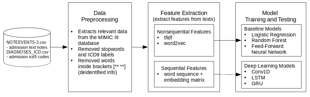
Figure 1: Methodology Pipeline Overview

3.1 Data Preprocessing

The MIMIC-III dataset is a large dataset relating to patients admitted to critical care units at a large tertiary care hospital. It contains de-identified medical records of patients who stayed from 2001 to 2012 within the intensive care units at Beth Israel Deaconess Medical Center [11]. The goal of this study is to explore useful semantic information using unstructured data. Therefore, only the free-text clinic note section from the dataset was used, specifically the noteevents table. Furthermore, the focus was on the discharge summaries category as it contained actual ground truth and free-text compared to other categories. Because discharge summaries were written after carrying out the diagnosis, the notes were sanitized by removing any mention of class-labels (ICD-9 codes). This approach is similar to the one utilized by Prakash et al. [23].

Table 1 describes the number of unique patients, hospital admissions, ICD-9 codes and ICD-9 categories involved in MIMIC-III dataset. All MIMIC-III describes the whole dataset, while noteevents and discharge summaries explain the corresponding subsets.

Coverage	Patients	Hospital Admissions	ICD-9 Codes	ICD-9 Categories
All MIMIC-III	46520	58976	6984	943
noteevents	46146	58361	6967	943
discharge summaries	41127	52726	6918	942

Table 1: MIMIC-III Descriptive Statistics

The data were preprocessed to produce separate datasets using two approaches. The first approach is to treat the ICD-9 code independently from each other, find the admissions (unique HADM_ID) for each ICD-9 classification, and consider only records related to the top 10 and top 50 common ICD-9 codes. The top 10 and top 50 were chosen because they covered a majority of the dataset (76.9% and 93.6% as illustrated in Table 3). The second approach is to group ICD-9 codes into categories based on their hierarchical nature, with categories for larger sets of similar health conditions (For instance, ”cholera due to vibrio cholerae” has the ICD-9 code 001.0, and is categorized as a type of cholera, which is also a type of intestinal infectious disease). The next step is to find the patients for top 10 and top 50 common categories. Evaluations would be separately performed on the four datasets, which will hereby be referred to as top-10-code, top-50-code, top-10-cat and top-50-cat, respectively.

Table 2 shows the top 10 ICD-9 codes and top 10 ICD-9 categories. Table 3 also describes the number of unique hospital admissions related to the four datasets mentioned in the previous paragraph.

ICD-9 Code	Admissions
4019: Hypertension	20046
4280: Congestive heart failure	12842
42731: Atrial fibrillation	12589
41401: Coronary atherosclerosis	12178
5849: Acute kidney failure	8906
25000: Diabetes Type II	8783
2724: Hyperlipidemia	8503
51881: Acute respiratory failure	7249
5990: Urinary tract infection	6442
53081: Esophageal reflux	6154

ICD-9 Category	Admissions
401: Essential hypertension	20646
427: Cardiac dysrhythmias	16774
276: Disorders of fluid electrolyte	14712
272: Disorders of lipoid metabolism	14212
414: Other chronic ischemic heart disease	14081
250: Diabetes mellitus	13818
428: Heart failure	13330
518: Other diseases of lung	12997
285: Other and unspecified anemias	12404
584: Acute kidney failure	11147

Table 2: Admission number for Top 10 ICD-9 codes and top 10 ICD-9 categories

Data Set	Hospital Admissions	discharge summaries Coverage (%)
top-10-code	40562	76.93%
top-50-code	49354	93.60%
top-10-cat	44419	84.24%
top-50-cat	51034	96.79%

Table 3: Dataset Descriptive Statistics

The filtered datasets will be split into 50-25-25 for training, validation and testing.

3.2 Feature Extraction

Two approaches will be used for feature extraction: They include Term Frequency - Inverse Document Frequency (tfidf) and word2vec [25]. The tfidf serves as a baseline of comparison with word2vec.

The tfidf aims to evaluate the level of importance of a word to a document in a collection of documents or corpus. It is the product of two statistics: tf and idf. While tf is the number of times a word appears in a given document, and idf measures whether a word is common or rare across the corpus. The following definition of idf will be used for our calculations:

$$idf(w)=log\frac{n_{d}}{df(d,w)}+1$$

where $n_{d}$ is the total number of documents, and $df(d,w)$ represents the number of documents that contain the word $w$.

To calculate tfidf, all the notes in the filtered training data set were first tokenized. Next, a document-word matrix with the count of each word in each note (tf) was created. Finally, each word was multiplied by the corresponding idf. Two tfidf configurations were also used: (1) one with top 40,000 words with highest tfidf scores as the bag of word features; (2) the other one with a minimum document frequency of 10 and a maximum document frequency of 0.8 of the total number of documents, which reduced the total number of words to around 20,000 words.

The model word2vec takes a tokenized text corpus as an input and produces word vectors as an output. The Continuous Bag of Words (CBOW) architecture was then used to predict the target word based on the context: words that precede and follow the target word. The CBOW is basically a Neural Network model that consists of inputs, projection and output layers where the traditional non-linear hidden layer is removed to reduce the time complexity and the projection layer is shared by all the words. The inputs are words in the context. We used text notes from MIMIC-III as corpus to train our word2vec model. Pre-trained word vectors induced from PubMed were also utilized. PubMed is a database of biomedical literature and the word vectors can be found at https://github.com/cambridgeltl/BioNLP-2016 [26]

3.3 Model Training and Testing

One fundamental assumption adopted by traditional supervised learning algorithms is that each sample has only one label assigned to it. In our problem, each sample has multiple (one or more) ICD-9 codes attached to it. Generally, there are two main methods for tackling the multi-label classification problem [27] One is the problem transformation methods and the other is algorithm adaptation methods. Problem transformation methods transform the multi-label problem into a set of binary classification or regression problems, and multiple binary classifiers are trained separately for each label. Algorithm adaptation methods, on the other hand, adapt the algorithms to perform multi-label classifications in its full form, and only one classifier is trained for all the labels.

In our study, three baseline approaches were first created: Linear Regression, Random Forests and Feed-forward Neural Networks. Then problem transformation methods were used to obtain the multi-label output for Linear Regression and Random Forests classifiers. Specifically, in order to assign each sample a set of target labels, $n$ different models for $n$ different labels were trained. Each model independently predicts a mutual exclusive output (0 or 1) for each sample data. For Feed-Forward Neural Networks, algorithm adaptation based methods were utilized, given that the neural network could be easily adapted to multi-label problem by setting up multiple neurons in the network output layer and each neuron represents a target label correspondingly. Similar to FNNs, algorithm adaptation-based methods were used in our deep learning models. In the following sub-sections, our implemented models will be described in detail.

3.3.1 Baseline Models

Logistic Regression (LR): Our first baseline model is a binomial logistic regression model implemented using Spark ML. For each label (ICD-9 code or category), a separate logistic regression model was trained, and each model independently predicted the said label (0 or 1 for the corresponding ICD-9 code or category). Different configurations were tried; specifically, “the number of iterations” was tuned between 5 to 100. Because only notes under discharge summaries category were used, there was one note per admission. Features extracted from this note were used as inputs for this classifier. For tfidf, the features were directly used as input features. For word2vec, the input features were the average of all the feature vectors of the words in the notes. This simple yet popular method was successfully applied in other studies to obtain sentence or document embedding [28, 29].

Random Forests (RFs): Our second baseline model is a random forest model implemented using Spark ML. The same approach and input for the logistic regression were used here (one model for each label). Different configurations were also evaluated; specifically the “tree depth” was tuned between 5 to 30.

Feed-forward Neural Networks (FNNs): One advantage of Neural Networks is that it can be fitted to multi-label problems in just one model with the proper activation function. The FNNs were implemented as the baseline for algorithm adaptation based multi-label classification problem (see Section 3.3). The same input features and train-test data split as previously described were used. The ReLU activation function was utilized for all the hidden layers and sigmoid function was used for the output layer, binary cross entropy as the loss function, and stochastic gradient descent as the optimizer. Several neural network models with one to four different hidden layers were also tried. For each hidden layer, a total of seven models was employed with the following combination of neuron sizes: 50, 100, 300, 500 and 1000. Among our model architectures, the best performed model pipeline is shown in Table 4.

Layer	0	1	2	3
NN	input	dense (ReLU)	dense (ReLU)	dense (ReLU)
Para	-	5000	500	100

Table 4: Configuration Details of the Best Performed FNN Architecture.

3.3.2 Deep Neural Network Models

In this study, the problem of ICD-9 code assignment from clinical notes was treated as multi-label classification problem on sequential observations $x_{1},x_{2},\cdots,x_{n}$, where $x_{i}$ is the word2vec features calculated for word $i$ in the discharge summary. Unlike the features used for the baseline models in which the sequential information was not preserved, each word was taken sequentially from the discharge summary. The input features for this classifier are $N$ most recent word sequences taken from the notes. If there were insufficient feature events, zero vectors were padded at the beginning. The word sequence was then converted into vectors using an embedding matrix based on a word2vec model (See Section 3.2).

Convolutional Neural Networks (CNNs) have achieved remarkable results in image processing related problems. In recent years, CNN models have shown excellent results for NLP such as in semantic parsing [30], search query retrieval [31], and sentence classification [32]. Thus, a series of experiments with CNNs were carried out. In general, the same architecture described in [32] was applied. As shown in Figure 2, the features were first concatenated into $n\times k$ feature vector, where $n$ is the number of words, and $k$ is the number of dimensions extracted from word2vec. A set of convolution filters with dimension $h\times k$ was then applied to a window of $h$ words to produce new features. The filters were then applied to each possible window of words in the sentences to produce a feature map. Finally, a max-overtime pooling operation over the feature map was applied to generate the fully connected layer. A sigmoid activation function was also applied to generate the multi-label output.

Figure 2: CNN Architecture

Various number of layers for our CNNs were tried, including three to ten convolutional (conv) layers with size 64, 128, or 256 for each layer. Then, each layer was followed with a max pooling layer, and one to three fully connected (fc) dense layers were attached to the last convolutional layer with a size of 4096, 1024 or 128. Among our model architecture setting, the best performed model pipeline is shown in Table 5. The same architecture was used on both top-10 and top-50 codes. Based on the hardware setting described, the training time for CNNs was less than 30 minutes with 500 maximum epochs and early stop if the validation loss did not improve for consecutive 10 epochs.

Layer	0	1	2	3	4	5	6	7
Architecture	input	conv	max pooling	conv	max pooling	conv	max pooling	fc
Para	-	128 - 5	5	128 - 5	5	128 - 5	35	128

Table 5: Configuration Details of the Best Performed CNN Architecture.

Recurrent Neural Networks (RNNs): RNNs are a type of neural network architecture designed to handle sequential inputs. They have shown promising results in many machine learning tasks [33]. Several RNN architectures were explored in this study. All the architectures follow the same pattern shown in Figure 3, where blue circles represent the text feature vectors. The green rectangles and the yellow rectangle represent recurrent hidden layers and the multi-label code assignment, respectively. Basically, the RNN cells went through the input sentences. Each word $x_{t}$ in the sentences generated a hidden layer $h_{t}$. Each hidden layer was connected with a directed connection weights $w_{h}$ to its successive layer $h_{t+1}$. The weights $w^{h}$ were shared among all the hidden layers (shared over time). The hidden layers of the RNN generated the outputs $\hat{y}$ when the RNN cells reached the last word. Sigmoid cross-entropy was then used as the loss function and RMSprop as the optimizer.

$$loss(\hat{y},y)=-\frac{1}{N}\sum_{n=1}^{l=N}y_{n}\cdot log(\hat{y_{n}})+(1-y_{n})\cdot log(1-\hat{y_{n}})$$

Figure 3: RNNs architecture

Although RNNs can handling input sequences of variable sizes, in practice, they face difficulties when modeling long-term dependencies [34]. To address this issue, various recurrent units were developed. Among those sophisticated recurrent units, in this study, two popular ones were evaluated: LSTMs [35] and Gated Recurrent Units (GRUs) [36]. Both of them could capture sequence-based inputs with long-term dependencies by utilizing a memory mechanism. Generally, LSTM contains three gates: the input gate, forget gate and output gate. The forget gate decides what information from previous and current input should be preserved or ignored. The input gate decides the values that will be updated to the cell states. The output gate decides what the next hidden state should be. A GRU is an LSTM without an output gate, and it uses an update gate to decide what past information should be kept and a reset gate decides how much past information should be discarded.

The input features to RNNs are the same as those used in CNNs. Three stacked recurrent layers with a combination 64, 128 and 256 units for each layer in our RNNs were tried. To predict the ICD-9 classification, only the output nodes of the last time step were considered, and the same activation function and loss function were applied as with the NNs. The best performed mode architecture for LSTMs and GRUs are shown in Table 6. Both architectures that performed best have two stacked recurrent layers with the same unit numbers for each layer. Based on the specified hardware setting, the training time was about 6 hours for GRUs and 18 hours for LSTMs with 200 maximum epochs and early stop if the validation loss did not improve for consecutive 5 epochs.

Layer	0	1	2	3	4	Layer	0	1	2	3	4
LSTMs	input	lstm	dropout	lstm	dropout	GRUs	input	gru	dropout	gru	dropout
Para	-	256	0.5	64	0.5	Para	-	256	0.5	64	0.5

Table 6: Configuration Details of the Best Performed LSTMs and GRUs Architectures.

3.4 Metrics

The combinations of our dataset, feature extraction methods, and models are evaluated under different performance metrics, including precision, accuracy, F-score and recall metrics for multi-label classification. Specifically, the following metrics are used [37]:

Precision $$=\frac{1}{n}\sum^{n}_{i=1}\frac{\lvert Y_{i}\cap Z_{i}\rvert}{\lvert Z_{i}\rvert} =\frac{1}{n}\sum^{n}_{i=1}\frac{\lvert Y_{i}\cap Z_{i}\rvert}{\lvert Y_{i}\rvert}$$ Recall

$$F_{1} =\frac{1}{n}\sum^{n}_{i=1}\frac{2\lvert Y_{i}\cap Z_{i}\rvert}{\lvert Y_{i}\rvert+\lvert Z_{i}\rvert} =\frac{1}{n}\sum^{n}_{i=1}\frac{\lvert Y_{i}\cap Z_{i}\rvert}{\lvert Y_{i}\cup Z_{i}\rvert}$$ Accuracy

where $Y_{i}$ is the set of predicted labels, $Z_{i}$ is the set of ground truth labels, and $n$ is the number of samples. Basically, precision calculates the proportion of predicted labels that are correct. Recall calculates the proportion of the actual labels that are correctly predicted. $F_{1}$ is the harmonic mean of precision and recall. Accuracy is the average proportion of the predicted correct labels to the total number of labels for all instances.

4 Results

This section illustrates the performance in three different aspects: (1) the baseline results, (2) the performance under different configurations, and (3) the best model performance.

4.1 Model Performance under Different Configurations

Different model configurations have been tried to give us insight into the most appropriate model configuration. Table 7 describes the different methods of feature extraction used and the parameters tweaked. The features extracted are divided into two categories: non-sequential and sequential features. The non-sequential features include tfidf and word2vec, both of which were used in Logistic Regression, Random Forests, and NNs. The sequential features includes word2seq (word sequences) used in conjunction with an embedding matrix based on word2vec, which were used in CNNs, RNNs, LSTMs, and GRUs. It is pertinent to note that we experimented on (1) using our custom word2vec model created from the MIMIC-III dataset and (2) utilizing pre-trained word vectors obtained from PubMed [26]. The vectors for stop words in the embedding matrix are all zeros.

Feature Extraction	Configuration	Value
tfidf	feature size	20301 - 40000
	minDocFreq	3 - 10
	max_df	0.8 - 1.0
word2vec	database	self trained from MIMIC-III (m3) or pre-trained from Pubmed (pm) [26]
	feature size	100 - 600
	pre-trained config	context window size 2 (win 2) or 30 (win30) [26]
wordseq	sequence length	1500-2000
	stopwords	removed from sequence or not removed
	embedding matrix	derived from the word2vec under different configurations

Table 7: Feature Extraction Methods

Figure 4 indicates the model performance of each model using different feature extraction methods on the top-10-code dataset. For each model, the configuration that provided the best performance here is used on the top-50-code, top-10-cat, and top-50-cat datasets. The results are further explained in the next section (see Section 4.2).

(a) Nonsequential

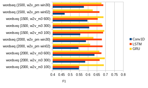
(b) Sequential

Figure 4: Model Performance under Different Configurations

Our three non-sequential models (Logistic Regression, Random Forests and NNs) had different but comparable performance depending on the features used. For example, for top-10 code classification, tfidf with 20k features produced the best $F_{1}$ results of 0.532 and 0.322 for Logistic Regression and Random Forests respectively. However, word2vec_m3 with 600 features produced the best results for FNNs with $F_{1}$ of 0.528 (although tfidf also gave a fairly good result for FNNs with $F_{1}$ of 0.488). Thus, tfidf configurations generated better results than those of word2vec. It is possible that the word2vec features lost information as the average of the word vectors was used to obtain document embedding for the non-sequential models. However, note that NNs gave fairly good results ($F_{1}$ 0.528) using the word2vec feature which was at most 600 dimensions compared to tfidf which was 20k or above. With a larger feature size, it is reasonable to say that tfidf kept a better global representation of document embedding. This ability could be used to explain the code classification. However, word2vec did retain the satisfactory representation of word embedding despite the substantial reduction in feature dimension (i.e., 20k down to 600).

Four sequential models (CNNs, simple RNNs, LTSMs and GRUs) were run under different configuration with two different types of embedding matrices (our self-trained word2vec from MIMIC-III corpus and pre-trained word2vec from PubMed [26]) and two sentence sequence lengths (1500 and 2000). In the top-10 code classification, seq. length 2000 + word2vec_m3 w/ 600 features generated the best $F_{1}$ result for CNNs, seq. length 1500 + word2vec_pm (win30) for LSTMs, and seq. length 2000 + word2vec_m3 w/ 300 features for GRUs. In short, all feature extraction methods generated good and comparable results for CNNs, LSTMs, and GRUs. Our self-trained word2vec also performed fairly well compared with the pre-trained word2vec models from PubMed. The best performed models with self-trained word2vec have $F_{1}$ of 0.637 (CNNs), 0.696 (GRUs) and 0.683 (LSTMs) while the best performed models from PubMed word2vec are 0.589 (CNNs), 0.677 (GRUs), and 0.687 (LSTMs). Under different configurations, our self-trained $word2vec$ outperformed PubMed word2vec in most cases. Experiments were also performed for simple RNNs. The results, however, were poor (0.0 - 0.08 $F_{1}$ at best). More information on this is explained in detail in Section 5. In addition, our top $F_{1}$ scores are linked to GRUs and LSTMs with GRUs providing slightly better results.

4.2 Best Model Performance

4.2.1 Overview

Figures 5 and 6 show the model performance, which is ordered from the best to worse, for the top-10-code, top-10-cat, top-50-code, and top-50-cat dataset. Figure 7 indicates the model performance for top-50-code and top-50-cat considering only the first 10 labels. Raw data are also shown in Tables 10 to 15 in the Appendix.

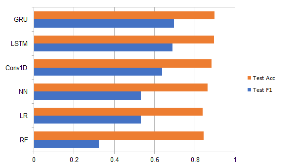
(a) top-10-code

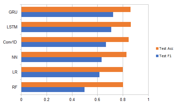
(b) top-10-cat

Figure 5: Model Performance Top 10

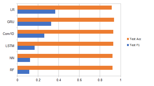
(a) top-50-code

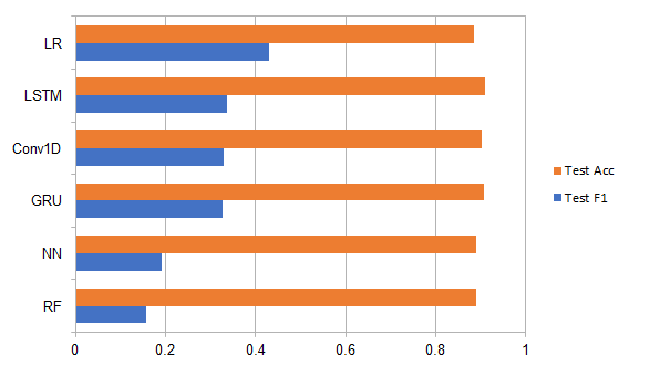
(b) top-50-cat

Figure 6: Model Performance Top 50

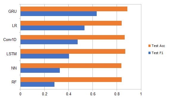
(a) top-50-code

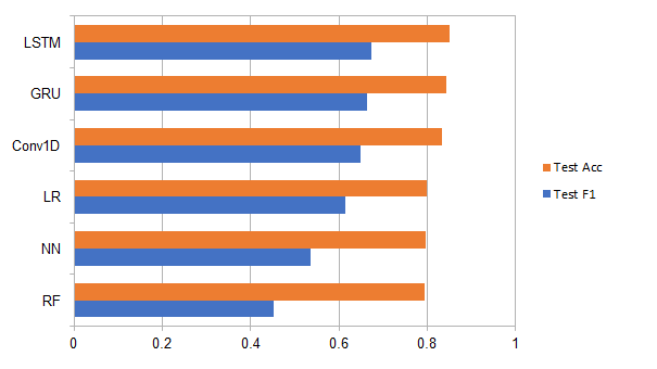
(b) top-50-cat

Figure 7: Model Performance Top 50 (first 10 labels only)

For top-10-code and top-10-cat, GRUs generated the best $F_{1}$ results (of 0.6957 and 0.7233, respectively). Hence, top-10-cat generated slightly better results than did top-10-code. This makes sense because there are more samples per label in top-10-cat and because the labels are less specific (the differences between labels are larger). Logistic Regression and Random Forests overfit the data with about 80% to 95% training $F_{1}$ but about 40% to 50% less on testing data). Even though FNNs are not overfitting, the results on testing data are slightly better than other baseline models. CNNs produces better results than FNNs, but there are more significant improvements with LSTMs and GRUs (about 70% $F_{1}$). This result signifies that our LSTMs and GRUs model can extract information from the sequence of words, thereby improving the $F_{1}$ and the result accuracy.

For top-50-code, Logistic Regression generated the best $F_{1}$ result of 0.3662. However, if only the first 10 labels are considered, GRUs generated the best $F_{1}$ result at 0.6328. For both all the label results and the first 10 label results, GRUs generated the best precision and accuracy results of 0.7520 and 0.8871, respectively. For top-50-cat, Logistic Regression also generated the best $F_{1}$ result of 0.4301. However, if only the first 10 labels are considered, LSTMs generated the best $F_{1}$ result of 0.6738. For both all the label results and the first 10 label results, GRUs generated the best precision and accuracy results of 0.7515 and 0.8345, respectively. Hence, top-50-cat generated slightly better results than did top-50-code. The baseline models (Logistic Regression and Random Forests) also overfit here.

4.2.2 Precision-Recall Curve

Table 8 presents the average overall precision performance of our selected best performance models for GRUs, LSTMs and CNNs. Average Precision (AP) summarizes the precision-recall curve as the mean of precisions achieved at different recall values and it is calculated as follows:

$$AP=\sum_{n}(R_{n}-R_{n-1})P_{n}$$

where $P_{n}$ and $R_{n}$ are the precision and recall at the nth threshold. As shown in the table below, GRUs generated the best precision results for top-10-code and top-50-code. Figure 8 shows precision-recall curve for the best-performed models for each label in top-10-code and the best-performing 10 labels for top-50-code. In this picture, it can be seen that for top-10-code, the top five common codes performed better than did the later ones. For example, the third common label (label 2: 42731), atrial fibrillation, has the highest AP of 0.90. followed by coronary atherosclerosis (label 3: 41401) with AP of 0.89, hypertension with AP of 0.83 (label 0: 4019) and congestive heart failure (label 1: 4280) with AP of 0.81. However, in the performance of top-50-code, it was observed that less common codes could also achieve high AP scores. For example, label 44: 7742, neonatal jaundice associated with preterm delivery, which have 2183 samples in the training dataset has the highest AP score of 0.92, and label 46: V053 with 2119 samples reached fifth. Other class-wise precision-recall curve for our tested models can be found in the Appendix.

Model	top-10-code	top-10-cat	top-50-code	top-50-cat	top-50-code(first10)	top-50-cat(first10)
LSTMs	0.7243	0.7915	0.3715	0.4929	0.7571	0.8426
GRUs	0.7362	0.7849	0.4518	0.4792	0.7949	0.8425
CNNs	0.6719	0.7293	0.3757	0.4565	0.7424	0.8269

Table 8: Average Precision Performance

(a) top-10-code

(b) top-50-code

Figure 8: Class-wise Precision-recall Curve for the Top 10 and the Best-performed 10 Labels for Top 50 Code Classification.

4.2.3 Results Comparison

Prakash and Zhao [23] used bag-of-words from discharge notes and Condensed Memory Neural Networks (C-MemNN) to tackle the same problem in this research. They tested their algorithm with top 50 and top 100 labels under metrics such as the macro average of Area Under the Curve (AUC), average precision over the top five predictions (Precision @5), and hamming loss.

$$AUC_{macro}=\frac{1}{q}\sum^{q}_{j=1}AUC_{j}$$

$$\textit{Hamming Loss}=\frac{1}{nq}\sum^{n}_{i=1}\sum^{q}_{j=1}xor(Z_{i,j},Y_{i,j})$$

where $AUC_{j}$ is the $AUC$ for each label, $q$ is the number of labels, and $n$ is the number of samples. Macro $AUC$ is used to calculate the unweighted mean of the $AUC$ values for each label. Hamming loss represents the fraction of labels that are incorrectly predicted. To compare our work with theirs, the same metrics were used for our best performed models for top 50 codes (top 100 labels are not compared), and the results are presented in Table 9.

Based on the results, it can be seen that while their hamming loss is better than ours, our work outperforms theirs in terms of macro AUC on GRU models and significantly performs better on top five precision for all of our models.

Model	AUC (macro)	Precision @5	Hamming Loss
C-MemNN [23]	0.833	0.42	0.01
GRUs	0.8599	0.8109	0.0645
LSTMs	0.8298	0.8054	0.0714
CNNs	0.8302	0.7998	0.0714

Table 9: Performance Comparison with Reference [23]

5 Discussion

Although some studies have used deep learning for automatic ICD-9 code assignment, a few of them have focused on getting meaningful information directly from unstructured clinical notes. Existing research on such tasks are difficult to compare with each other because there is a lack of standard comparison metrics. This study is significant in that it conducted extensive experiments to examine the performance of popular machine learning and deep learning algorithms under a set of standard metrics, precision, recall, $F_{1}$ and accuracy. As the output label vector for our task was sparse (for each sample, only a few labels were generally active), the influence of sparsity was considered when choosing the measurements. For instance, both hamming loss and accuracy are in favor of sparse labels. An all-zero classifier would have the hamming loss close to 0 and the accuracy close to 1. Precision, recall, and $F_{1}$ are more reasonable choices compared to hamming loss and accuracy. If the developed system is aiming for recommendation, $Precision@k$ has often been used for such purpose [38]. Other optimized measures for sparse labels are also worth exploring in future research [39].

Our findings support the use of RNNs for code assignment on patient notes, as they show better performance than other machine learning models as well as previously published systems [23] under certain metrics. Except from the sequential RNN models, the other models only consider the current input and they have no notion of order in time. They simply can not remember anything about what happened in the past. In a FNN, the information moves straight through the network in one direction. Because of that, the information hardly touches a node twice. In contrast, RNNs try to derive relations from the current word and what it has learned from previous words in the same sentence. In RNNs, each node at a time step takes an input from the previous node using a feedback loop.

To further understand what form of deep neural network architecture works better on automatic ICD-9 coding, the performance of CNNs, simple RNNs, and RNNs with long-term dependencies capability were also compared. Among all the compared methods (including the baseline models), simple RNNs without memory mechanism produced the worst performance. The $F_{1}$ is 0.08 at best for various configurations. Although it is well known that RNNs can only use information from near past, the unsatisfactory results may be due to the learning ability of the network itself. As explained in [34], RNNs for tasks with long-term dependencies would not be robust to input noise or would not be efficiently trainable by gradient descent, and the gradient of the loss function decays exponentially with time. Worth noting is that in order to know if representations from future time steps would help the network to gain extra information, bidirectional LSTMs and GRUs were also implemented in our experiments. Bidirectional RNNs connects two hidden layers of opposite directions to the same output. Such mechanisms make the network receive information from past and future states simultaneously. Bidirectional RNNs are especially useful when the later context of the input is needed. It was observed that bidirectional RNNs do not outperform (comparable or slightly worse) the RNNs for the top-10 code assignment task. Considering the extra computation cost of the bidirectional RNNs, this network architecture was not further explored with the belief that peeking future information may not beneficial to our task.

Despite the fact that CNNs did not perform as good as LSTMs and GRUs, the training time for CNNs (30 minutes) was significantly less than that of GRUs (6 hours) and LSTMs (18 hours). The computation for CNNs can happen in parallel, while RNNs need to be processed sequentially, After all, the subsequent steps depend on previous ones. As part of future work, the results may be improved with newly designed network architectures, such as Temporal Convolutional Networks (TCNs) [40]. Bai et al. compared a series of benchmark competitions of TCNs versus RNNs, LSTMs, and GRUs across eleven different industry standard RNNs problems. They found that TCN models substantially outperformed generic recurrent architectures such as LSTMs and GRUs. They also showed that TCNs exhibited longer memory than did recurrent architectures with the same capacity [41].

The paper also evaluates the impact of word embedding on the performance of our tested methods. For baseline models, a simple yet popular method to generate the non-sequential word2vec feature vector was used. Specifically, the word vectors from a discharge summary were averaged. Models using the averaged word vector features performed worse than those using tfidf features. While for deep learning, because the sequential information can be retained, almost all the networks with word2vec could generate better results than our baseline models. In addition, compared to our self-trained word2vec from MIMIC-III and word2vec downloaded from PubMed, they showed comparable performance and the word2vec trained from MIMIC-III generally produced slightly better results.

Although LSTMs and GRUs could capture long-term dependencies, the length of our input sequence could still be too long for LSTMs and GRUs to retain useful information. A different representation may be used to shorten the sequence, e.g. sentence2vec or paragraph2vec [42]. In addition to that, based on the comparison in Section 4.2.3, memory networks provide better results for certain metrics. word2vec representation and memory network can help address this problem.

Our current models for top 50 ICD-9 codes and categories were not successful. This failure may be because our current model design could not effectively distinguish between 50 different labels. To improve our model capability, we could run five top-10 models in parallel (each model predicting 10 labels), thereby making our top-50 models have the same model capability as our top-10 models. It was also observed that the samples for labels 11 to 50 were greatly imbalanced (i.e., the positive samples where very few compared to negative samples). Hence, the data might not be sufficient for the deep neural network to learn adequate useful representations. As part of future work, the sample size of the clinical notes that contains those labels needs to be balanced or increased. Zeng et al. [22] also showed that deep transfer learning could improve the performance of automatic ICD-9 coding on labels with limited samples.

Our custom word2vec model used CBOW. Skip-gram (even though the pre-trained word2vec induced from PubMed are skip-gram based) was not used. Some previous studies have noted that skip-gram outperforms CBOW in biomedical domain tasks [26]. Therefore, in future work, the effect of different word2vec parameters on our ICD-9 code or category classifier will be further explored.

Further research on what words affect the probability of a prediction could improve our understanding of the relationship between symptoms and diagnosis. The probability observation could also change our preprocessing and feature extraction methods and ultimately improve our deep learning models.

6 Conclusion

This study evaluates different NLP deep learning based models and feature extraction methods. It also establishes an empirical evaluation for learning-based automatic code assignment from the MIMIC-III discharge summary. The models are based on deep learning NLP frameworks that automatically assign clinical ICD-9 codes from free-text clinical notes. The deep learning models for predicting the top 10 ICD-9 codes and categories performed better than our baseline models that used traditional learning algorithms (best $F_{1}$ results: 0.6957 GRUs to 0.5320 Logistic Regression, and 0.7233 GRUs to 0.6313 FNNs, respectively). It was observed that the top 50 ICD-9 codes and categories results did not outperform our baseline ($F_{1}$ results: 0.3263 GRUs compared to 0.3662 Logistic Regression, and 0.3367 GRUs compare to 0.3651 FNNs). We believe that with more descriptive record collection and modern deep learning strategies, the predictive ability will likely increase. We also hope that our implementation and evaluation of the current state-of-the-art algorithms will serve as a baseline for further research on this topic.

Conflict of Interest Statement

The authors declare that there is no conflict of interest. The authors do not have financial and personal relationships with other people or organizations that could inappropriately influence (bias) their work.

Appendix A Model Performance for Top 10 Label Codes

	Training				Test
Model	Precision	Recall	Accuracy	$F_{1}$	Precision	Recall	Accuracy	$F_{1}$
Logistic Regression	0.9564	0.9440	0.9786	0.9501	0.5801	0.4934	0.8392	0.5320
Random Forests	0.9989	0.6988	0.9501	0.8086	0.7573	0.2340	0.8432	0.3219
Feed-forward NN	0.7933	0.5742	0.8998	0.6457	0.6810	0.4634	0.8622	0.5323
CNNs	0.8312	0.6713	0.9165	0.7371	0.7408	0.5687	0.8832	0.6373
LSTM RNNs	0.8106	0.6971	0.9154	0.7445	0.7574	0.6380	0.8950	0.6874
GRU RNNs	0.7936	0.6971	0.9126	0.7397	0.7502	0.6519	0.8967	0.6957

Table 10: Model Performance for top-10-code

Appendix B Model Performance for Top 50 Codes

	Training				Test
Model	Precision	Recall	Accuracy	$F_{1}$	Precision	Recall	Accuracy	$F_{1}$
Logistic Regression	0.9863	0.9768	0.9945	0.9815	0.4372	0.3213	0.9148	0.3662
Random Forests	0.9985	0.2852	0.9451	0.3866	0.5377	0.0953	0.9220	0.1155
Feed-forward NN	0.2490	0.1138	0.9224	0.1268	0.2251	0.1090	0.9212	0.1215
CNNs	0.6085	0.2663	0.9365	0.3200	0.4792	0.2169	0.9286	0.2609
LSTM RNNs	0.3526	0.1642	0.9325	0.1891	0.4022	0.1445	0.9286	0.1659
GRU RNNs	0.6539	0.3433	0.9460	0.3947	0.5592	0.2782	0.9354	0.3263

Table 11: Model Performance for top-50-code

	Training				Test
Model	Precision	Recall	Accuracy	$F_{1}$	Precision	Recall	Accuracy	$F_{1}$
Logistic Regression	0.9564	0.9440	0.9786	0.9501	0.5801	0.4934	0.8392	0.5320
Random Forests	0.9946	0.4937	0.9110	0.6305	0.7869	0.2009	0.8395	0.2822
Feed-forward NN	0.5266	0.2783	0.8408	0.3380	0.5143	0.2676	0.8370	0.3276
CNNs	0.7708	0.4673	0.8858	0.5377	0.6784	0.4109	0.8650	0.4739
LSTM RNNs	0.6204	0.3829	0.8805	0.4348	0.5748	0.3526	0.8688	0.4025
GRU RNNs	0.8351	0.6474	0.9168	0.7181	0.7520	0.5618	0.8871	0.6328

Table 12: Model Performance for top-50-code (first 10)

Appendix C Model Performance for Top 10 Label Categories

	Training				Test
Model	Precision	Recall	Accuracy	$F_{1}$	Precision	Recall	Accuracy	$F_{1}$
Logistic Regression	0.9437	0.9309	0.9652	0.9372	0.6458	0.5856	0.7994	0.6141
Random Forests	0.9983	0.8134	0.9500	0.8954	0.7653	0.3801	0.8019	0.4966
Feed-forward NN	0.7989	0.6456	0.8632	0.7083	0.7334	0.5633	0.8272	0.6314
CNNs	0.8039	0.6637	0.8681	0.7128	0.7613	0.6126	0.8446	0.6657
LSTM RNNs	0.8146	0.6807	0.8749	0.7343	0.7926	0.6536	0.8622	0.7090
GRU RNNs	0.8150	0.7613	0.8909	0.7861	0.7580	0.6941	0.8588	0.7233

Table 13: Model Performance for top-10-cat

Appendix D Model Performance for Top 50 Label Categories

	Training				Test
Model	Precision	Recall	Accuracy	$F_{1}$	Precision	Recall	Accuracy	$F_{1}$
Logistic Regression	0.9750	0.9572	0.9887	0.9659	0.4858	0.3894	0.8841	0.4301
Random Forests	0.9986	0.3294	0.9277	0.4465	0.6568	0.1142	0.8906	0.1576
Feed-forward NN	0.3522	0.1654	0.8940	0.2007	0.3600	0.1557	0.8909	0.1901
CNNs	0.7428	0.3262	0.9163	0.3870	0.5635	0.2770	0.9035	0.3301
LSTM RNNs	0.7117	0.3363	0.9194	0.3804	0.5869	0.2945	0.9087	0.3367
GRU RNNs	0.6695	0.3227	0.9179	0.3726	0.5611	0.2809	0.9067	0.3266

Table 14: Model Performance for top-50-cat

	Training				Test
Model	Precision	Recall	Accuracy	$F_{1}$	Precision	Recall	Accuracy	$F_{1}$
Logistic Regression	0.9437	0.9309	0.9652	0.9372	0.6458	0.5856	0.7994	0.6141
Random Forests	0.9937	0.6321	0.8999	0.7687	0.7877	0.3282	0.7944	0.4512
Feed-forward NN	0.6905	0.4762	0.8043	0.5535	0.6795	0.4562	0.7955	0.5347
CNNs	0.7945	0.6652	0.8670	0.7142	0.7296	0.5979	0.8345	0.6481
LSTM RNNs	0.7963	0.6863	0.8768	0.7213	0.7515	0.6362	0.8514	0.6738
GRU RNNs	0.7901	0.6803	0.8729	0.7213	0.7382	0.6196	0.8442	0.6641

Table 15: Model Performance for top-50-cat (first 10)

Appendix E Best Performance Models (LSTMs, GRUs, CNNs) Precision-Recall Curve

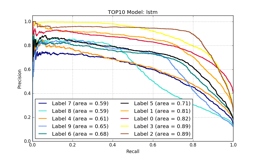
(a) LSTMs Top 10 Codes

(b) LSTMs Top 10 Categories

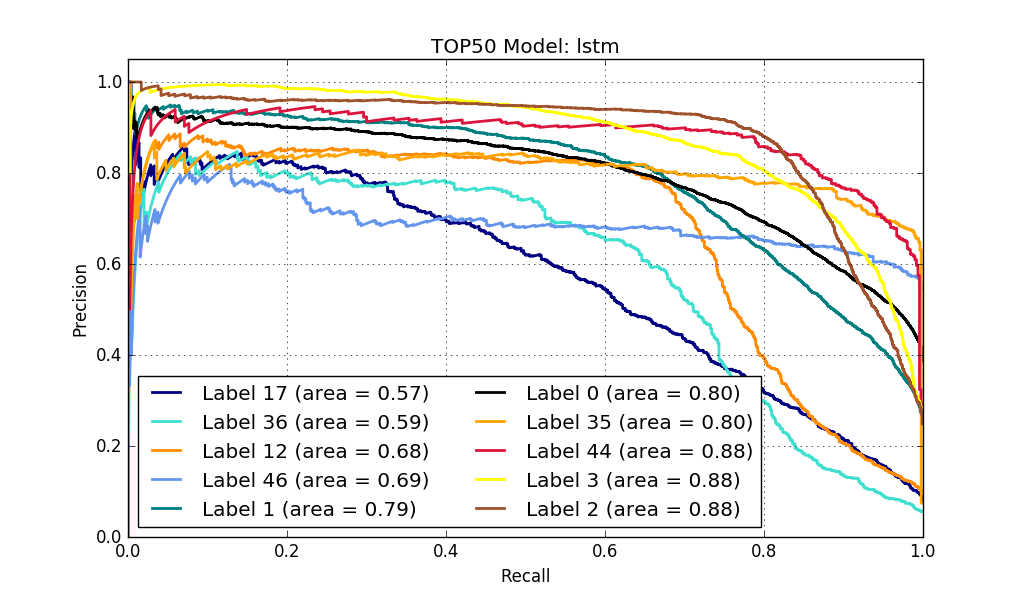
(c) LSTMs Top 50 Codes

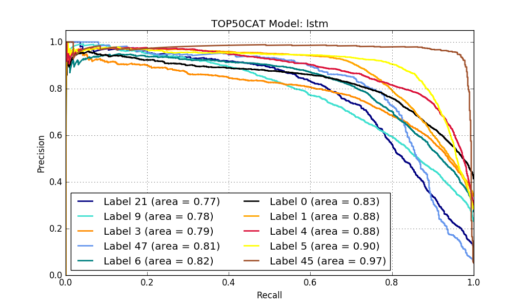
(d) LSTMs Top 50 Categories

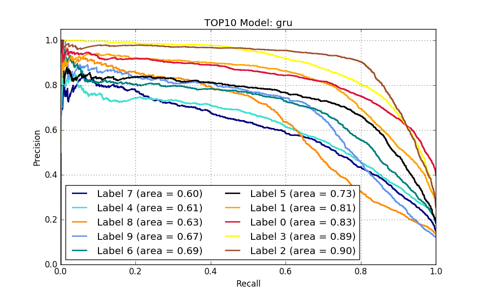
(e) GRUs Top 10 Codes

(f) GRUs Top 10 Categories

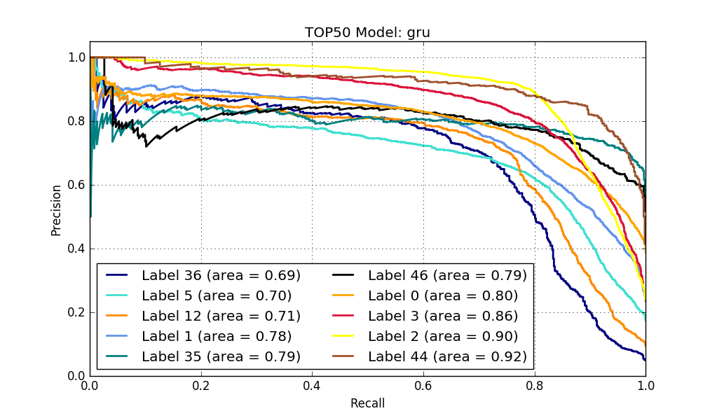
(g) GRUs Top 50 Codes

(h) GRUs Top 50 Categories

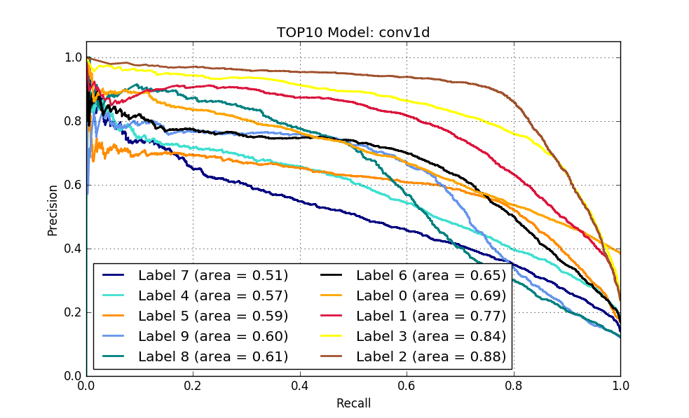
(i) CNNs Top 10 Codes

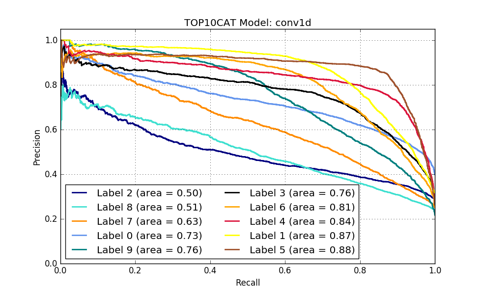
(j) CNNs Top 10 Categories

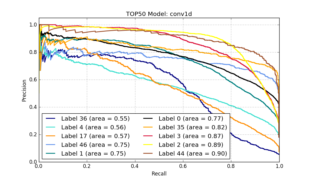
(k) CNNs Top 50 Codes

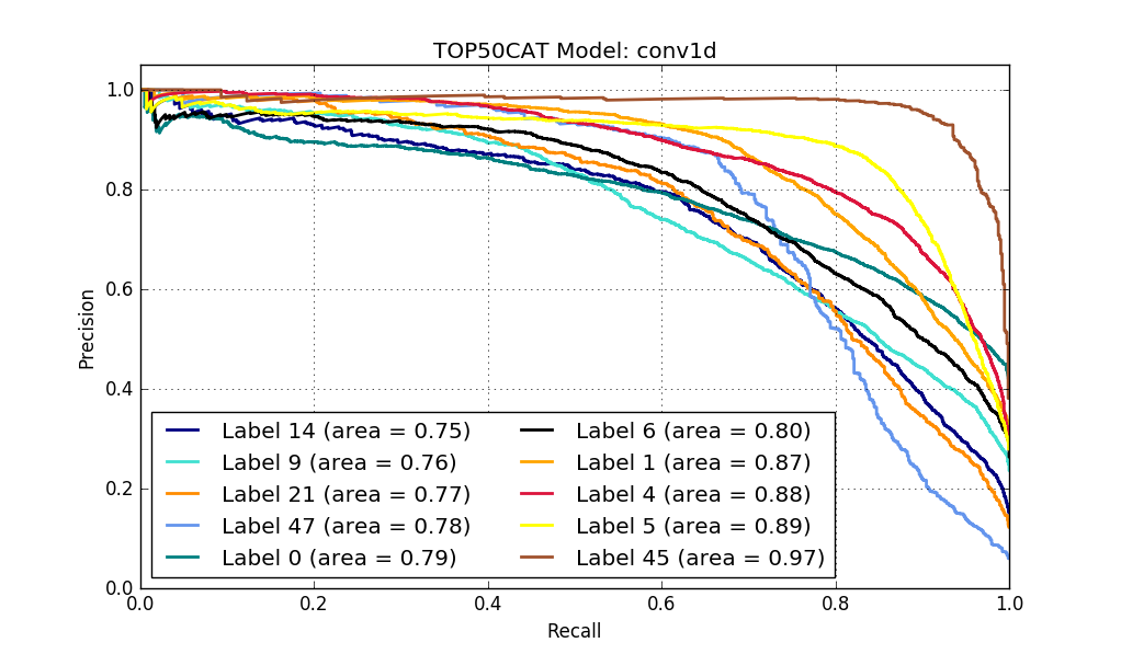
(l) CNNs Top 50 Categories

References

- [1] Ashly D Black, Josip Car, Claudia Pagliari, Chantelle Anandan, Kathrin Cresswell, Tomislav Bokun, Brian McKinstry, Rob Procter, Azeem Majeed, and Aziz Sheikh. The impact of ehealth on the quality and safety of health care: a systematic overview. PLoS Med, 8(1):e1000387, 2011.
- [2] Edward Choi, Mohammad Taha Bahadori, Andy Schuetz, Walter F Stewart, and Jimeng Sun. Doctor ai: Predicting clinical events via recurrent neural networks. In Machine Learning for Healthcare Conference, pages 301–318, 2016.
- [3] F Martin-Sanchez, K Verspoor, et al. Big data in medicine is driving big changes. Yearb Med Inform, 9(1):14–20, 2014.
- [4] Jose C Ferrao, Filipe Janela, Monica D Oliveira, and Henrique MG Martins. Using structured ehr data and svm to support icd-9-cm coding. In Healthcare Informatics (ICHI), 2013 IEEE International Conference on, pages 511–516. IEEE, 2013.
- [5] Serguei VS Pakhomov, James D Buntrock, and Christopher G Chute. Automating the assignment of diagnosis codes to patient encounters using example-based and machine learning techniques. Journal of the American Medical Informatics Association, 13(5):516–525, 2006.
- [6] Julia Medori and Cédrick Fairon. Machine learning and features selection for semi-automatic icd-9-cm encoding. In Proceedings of the NAACL HLT 2010 Second Louhi Workshop on Text and Data Mining of Health Documents, pages 84–89. Association for Computational Linguistics, 2010.
- [7] Ira Goldstein, Anna Arzumtsyan, and Özlem Uzuner. Three approaches to automatic assignment of icd-9-cm codes to radiology reports. In AMIA Annual Symposium Proceedings, volume 2007, page 279. American Medical Informatics Association, 2007.
- [8] Ilya Sutskever, Oriol Vinyals, and Quoc V Le. Sequence to sequence learning with neural networks. In Advances in neural information processing systems, pages 3104–3112, 2014.
- [9] Ronan Collobert, Jason Weston, Léon Bottou, Michael Karlen, Koray Kavukcuoglu, and Pavel Kuksa. Natural language processing (almost) from scratch. Journal of Machine Learning Research, 12(Aug):2493–2537, 2011.
- [10] Richard Socher, Jeffrey Pennington, Eric H Huang, Andrew Y Ng, and Christopher D Manning. Semi-supervised recursive autoencoders for predicting sentiment distributions. In Proceedings of the conference on empirical methods in natural language processing, pages 151–161. Association for Computational Linguistics, 2011.
- [11] Alistair EW Johnson, Tom J Pollard, Lu Shen, H Lehman Li-wei, Mengling Feng, Mohammad Ghassemi, Benjamin Moody, Peter Szolovits, Leo Anthony Celi, and Roger G Mark. Mimic-iii, a freely accessible critical care database. Scientific data, 3:160035, 2016.
- [12] Leah S Larkey and W Bruce Croft. Automatic assignment of icd9 codes to discharge summaries. Technical report, Technical report, University of Massachusetts at Amherst, Amherst, MA, 1995.
- [13] John P Pestian, Christopher Brew, Paweł Matykiewicz, Dj J Hovermale, Neil Johnson, K Bretonnel Cohen, and Włodzisław Duch. A shared task involving multi-label classification of clinical free text. In Proceedings of the Workshop on BioNLP 2007: Biological, Translational, and Clinical Language Processing, pages 97–104. Association for Computational Linguistics, 2007.
- [14] Berthier Ribeiro-Neto, Alberto HF Laender, and Luciano RS De Lima. An experimental study in automatically categorizing medical documents. Journal of the Association for Information Science and Technology, 52(5):391–401, 2001.
- [15] Stéphane M Meystre, Guergana K Savova, Karin C Kipper-Schuler, John F Hurdle, et al. Extracting information from textual documents in the electronic health record: a review of recent research. Yearb Med Inform, 35(128):44, 2008.
- [16] Yuan Ling. Methods and Techniques for Clinical Text Modeling and Analytics. PhD thesis, Drexel University, 2017.
- [17] Alex Krizhevsky, Ilya Sutskever, and Geoffrey E Hinton. Imagenet classification with deep convolutional neural networks. In Advances in neural information processing systems, pages 1097–1105, 2012.
- [18] Alex Graves, Abdel-rahman Mohamed, and Geoffrey Hinton. Speech recognition with deep recurrent neural networks. In Acoustics, speech and signal processing (icassp), 2013 ieee international conference on, pages 6645–6649. IEEE, 2013.
- [19] Edward Choi, Andy Schuetz, Walter F Stewart, and Jimeng Sun. Using recurrent neural network models for early detection of heart failure onset. Journal of the American Medical Informatics Association, page ocw112, 2016.
- [20] Zachary C Lipton, David C Kale, Charles Elkan, and Randall Wetzell. Learning to diagnose with lstm recurrent neural networks. arXiv preprint arXiv:1511.03677, 2015.
- [21] Edward Choi, Mohammad Taha Bahadori, Jimeng Sun, Joshua Kulas, Andy Schuetz, and Walter Stewart. Retain: An interpretable predictive model for healthcare using reverse time attention mechanism. In Advances in Neural Information Processing Systems, pages 3504–3512, 2016.
- [22] Min Zeng, Min Li, Zhihui Fei, Ying Yu, Yi Pan, and Jianxin Wang. Automatic icd-9 coding via deep transfer learning. Neurocomputing, 324:43–50, 2019.
- [23] Aaditya Prakash, Siyuan Zhao, Sadid A Hasan, Vivek V Datla, Kathy Lee, Ashequl Qadir, Joey Liu, and Oladimeji Farri. Condensed memory networks for clinical diagnostic inferencing. In AAAI, pages 3274–3280, 2017.
- [24] Benjamin Shickel, Patrick James Tighe, Azra Bihorac, and Parisa Rashidi. Deep ehr: a survey of recent advances in deep learning techniques for electronic health record (ehr) analysis. IEEE journal of biomedical and health informatics, 22(5):1589–1604, 2018.
- [25] Tomas Mikolov, Ilya Sutskever, Kai Chen, Greg S Corrado, and Jeff Dean. Distributed representations of words and phrases and their compositionality. In Advances in neural information processing systems, pages 3111–3119, 2013.
- [26] Billy Chiu, Gamal Crichton, Anna Korhonen, and Sampo Pyysalo. How to train good word embeddings for biomedical nlp. Proceedings of the 15th Workshop on Biomedical Natural Language Processing, pages 166–174, 2016.
- [27] Grigorios Tsoumakas and Ioannis Katakis. Multi-label classification: An overview. International Journal of Data Warehousing and Mining (IJDWM), 3(3):1–13, 2007.
- [28] Manaal Faruqui, Jesse Dodge, Sujay Kumar Jauhar, Chris Dyer, Eduard Hovy, and Noah A Smith. Retrofitting word vectors to semantic lexicons. In Proceedings of the 2015 Conference of the North American Chapter of the Association for Computational Linguistics: Human Language Technologies, pages 1606–1615, 2015.
- [29] Tom Kenter, Melvin Wevers, Pim Huijnen, and Maarten de Rijke. Ad hoc monitoring of vocabulary shifts over time. In Proceedings of the 24th ACM International on Conference on Information and Knowledge Management, pages 1191–1200. ACM, 2015.
- [30] Wen-tau Yih, Kristina Toutanova, John C Platt, and Christopher Meek. Learning discriminative projections for text similarity measures. In Proceedings of the Fifteenth Conference on Computational Natural Language Learning, pages 247–256. Association for Computational Linguistics, 2011.
- [31] Yelong Shen, Xiaodong He, Jianfeng Gao, Li Deng, and Grégoire Mesnil. Learning semantic representations using convolutional neural networks for web search. In Proceedings of the 23rd International Conference on World Wide Web, pages 373–374. ACM, 2014.
- [32] Yoon Kim. Convolutional neural networks for sentence classification. In Proceedings of the 2014 Conference on Empirical Methods in Natural Language Processing (EMNLP), pages 1746–1751, 2014.
- [33] Alex Graves et al. Supervised sequence labelling with recurrent neural networks, volume 385. Springer, 2012.
- [34] Yoshua Bengio, Patrice Simard, and Paolo Frasconi. Learning long-term dependencies with gradient descent is difficult. IEEE transactions on neural networks, 5(2):157–166, 1994.
- [35] Sepp Hochreiter and Jürgen Schmidhuber. Long short-term memory. Neural computation, 9(8):1735–1780, 1997.
- [36] Kyunghyun Cho, Bart van Merriënboer, Dzmitry Bahdanau, and Yoshua Bengio. On the properties of neural machine translation: Encoder–decoder approaches. Syntax, Semantics and Structure in Statistical Translation, page 103, 2014.
- [37] Min-Ling Zhang and Zhi-Hua Zhou. A review on multi-label learning algorithms. IEEE transactions on knowledge and data engineering, 26(8):1819–1837, 2014.
- [38] Rahul Agrawal, Archit Gupta, Yashoteja Prabhu, and Manik Varma. Multi-label learning with millions of labels: Recommending advertiser bid phrases for web pages. In Proceedings of the 22nd international conference on World Wide Web, pages 13–24. ACM, 2013.
- [39] Krzysztof Dembczyński, Willem Waegeman, Weiwei Cheng, and Eyke Hüllermeier. On label dependence and loss minimization in multi-label classification. Machine Learning, 88(1-2):5–45, 2012.
- [40] Colin Lea, Michael D Flynn, Rene Vidal, Austin Reiter, and Gregory D Hager. Temporal convolutional networks for action segmentation and detection. In proceedings of the IEEE Conference on Computer Vision and Pattern Recognition, pages 156–165, 2017.
- [41] Shaojie Bai, J. Zico Kolter, and Vladlen Koltun. An empirical evaluation of generic convolutional and recurrent networks for sequence modeling. arXiv:1803.01271, 2018.
- [42] Quoc Le and Tomas Mikolov. Distributed representations of sentences and documents. In International Conference on Machine Learning, pages 1188–1196, 2014.