Quantum-optimal detection of one-versus-two incoherent optical sources with arbitrary separation

Abstract

We analyze the fundamental quantum limit of the resolution of an optical imaging system from the perspective of the detection problem of deciding whether the optical field in the image plane is generated by one incoherent on-axis source with brightness $\epsilon$ or by two $\epsilon/2$-brightness incoherent sources that are symmetrically disposed about the optical axis. Using the exact thermal-state model of the field, we derive the quantum Chernoff bound for the detection problem, which specifies the optimum rate of decay of the error probability with increasing number of collected photons that is allowed by quantum mechanics. We then show that recently proposed linear-optic schemes approach the quantum Chernoff bound—the method of binary spatial-mode demultiplexing (B-SPADE) is quantum-optimal for all values of separation, while a method using image-inversion interferometry (SLIVER) is near-optimal for sub-Rayleigh separations. We then simplify our model using a low-brightness approximation that is very accurate for optical microscopy and astronomy, derive quantum Chernoff bounds conditional on the number of photons detected, and show the optimality of our schemes in this conditional detection paradigm. For comparison, we analytically demonstrate the superior scaling of the Chernoff bound for our schemes with source separation relative to that of spatially-resolved direct imaging. Our schemes have the advantages over the quantum-optimal (Helstrom) measurement in that they do not involve joint measurements over multiple modes, and that they do not require the angular separation for the two-source hypothesis to be given a priori and can offer that information as a bonus in the event of a successful detection.

The influential Rayleigh criterion for imaging resolution LordRayleigh1879 , which specifies a minimum separation for two incoherent light sources to be distinguishable by a given imaging system, is based on heuristic notions. As pointed out by Feynman (Feynman1963, , Sec. 30–4): “Rayleigh’s criterion is a rough idea in the first place …” and a better resolution can be achieved “… if sufficiently careful measurements of the exact intensity distribution over the diffracted image spot can be made …” The fundamental measurement noise is the quantum noise necessarily accompanying any measurement. A more rigorous approach to the resolution measure that accounts for the quantum noise in ideal spatially-resolved image-plane photon counting can be formulated using the classical Cramér-Rao bound on the minimum estimation error for locating the sources Ram2006 ; Chao2016 . Very recently, using methods of quantum estimation theory Helstrom1976 ; Holevo1982 , it was found that the estimation of the separation between two incoherent sources below the Rayleigh criterion can be drastically improved by measurements employing pre-detection linear optic processing of the collected light, followed by photon counting Tsang2016b ; Nair2016 ; Tsang2016a ; Nair2016a ; Ang2016 ; Lupo2016 ; Rehacek2016 ; Tsang2016c ; KGA17 ; YNT+17 ; Tang2016 ; Yang2016 ; Tham2017 ; Paur2016 .

Besides the minimum error of estimating the separation of two point sources, the resolving power of an imaging system can also be studied via the paradigmatic detection problem of deciding whether the optical field in the image plane is generated by one source or two sources Harris1964 ; Helstrom1973 ; Acuna1997 ; Shahram2006 ; Dutton2010 . This detection perspective is especially relevant to the detection of binary stars and exoplanets Acuna1997 ; Labeyrie2006 and the detection of protein multimers with fluorescent microscopes Nan2013 . In a pioneering work Helstrom1973 , Helstrom obtained the mathematical description of the quantum-optimal measurement that minimizes the error probability for detecting one or two point sources emitting quasi-monochromatic thermal light. Unfortunately, in addition to having no known physical realization, his method requires the separation between the two hypothetical sources to be given, though this separation is usually unknown in practice.

Here we investigate the performance of two practical quantum measurements for the detection of weak incoherent quasi-monochromatic point light sources. We assess the performance of these measurements vis-a-vis direct imaging and the optimum quantum measurement using the asymptotic error exponent (or Chernoff exponent), which specifies the rate at which the error probability decreases exponentially as the observation time or number of received photons increases. We show that a binary spatial-mode demultiplexing (B-SPADE) scheme Tsang2016b is quantum-optimal for all values of separations in the following two senses: (1) the asymptotic error exponent attains the maximum allowed by quantum mechanics, and (2) the error probability of a simple decision rule based on the observations of the B-SPADE is close to the quantum limit. We also show that the scheme of superlocalization by image inversion interferometry (SLIVER) Nair2016 ; Nair2016a is near-optimal for sub-Rayleigh separations. The Chernoff exponents of both schemes are shown to be superior to that of ideal shot-noise-limited continuum direct imaging in the sub-Rayleigh regime. In addition to their superiority over direct imaging, our methods do not require the capability to perform joint quantum measurements, do not require the two-source separation to be known a priori, can offer an accurate estimate of this separation in the event of a successful detection Tsang2016b ; Nair2016 ; Tsang2016a ; Nair2016a ; Ang2016 ; Lupo2016 ; Rehacek2016 ; Tsang2016c , and rely on methods that have been experimentally demonstrated in the context of parameter estimation Tang2016 ; Yang2016 ; Tham2017 ; Paur2016 . These advantages over the Helstrom measurement Helstrom1973 hold tremendous promise for practical detection applications in both astronomy Acuna1997 and molecular imaging Nan2013 .

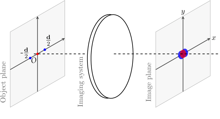
Figure 1: Schematic of the imaging of incoherent point light sources by a spatially-invariant imaging system. The images of two point sources of equal brightness (blue) spaced closer than the width of the point-spread function (PSF) of the imaging system are difficult to distinguish from that of one point source of the same total brightness (red) located midway between them.

Results
One source versus two sources. The set-up considered in this work is illustrated in Fig. 1. Under hypothesis $\textsf{H}_{1}$, we have a single thermal source of brightness (average photon number per temporal mode) $\epsilon$ imaged at the origin of the image plane. Under hypothesis $\textsf{H}_{2}$, we have two thermal sources, each of strength $\epsilon/2$, located a distance $d$ apart and imaged at the points $\pm\mathbf{d}/2=(\pm d/2,0)$ in the image plane. To focus on the resolution power of an optical imaging system, the total brightness is assumed to be identical under the two hypotheses so that simple photon counting is ineffective as a decision strategy. Similarly, the sources are presumed to have identical frequency spectra so that spectroscopy cannot help to distinguish the hypotheses. A strategy for accepting one or the other hypothesis, known as a decision rule, is given by partitioning the space of observations $\mathcal{Z}$ (which is determined by the choice of measurement) into two disjoint regions $\mathcal{Z}_{1}$ and $\mathcal{Z}_{2}$; the one-source hypothesis $\mathsf{H}_{1}$ is accepted if the observation belongs to $\mathcal{Z}_{1}$, and $\mathsf{H}_{2}$ is accepted otherwise. The performed quantum measurement can be described by a positive-operator-valued measure (POVM) $\{E(z)\}_{z\in\mathcal{Z}}$, where $z$ denotes the outcome, and the $E(z)$’s are nonnegative operators resolving the identity operator as $\int\!{\rm d}\mu(z)E(z)=\openone$ with $\mu(z)$ being an appropriate measure on $\mathcal{Z}$ Helstrom1976 ; Holevo1982 ; Hayashi2006 . Define $E_{1}=\int_{z\in\mathcal{Z}_{1}}\!{\rm d}\mu(z)E(z)$ and $E_{2}=\int_{z\in\mathcal{Z}_{2}}\!{\rm d}\mu(z)E(z)$. Let $\rho_{1}$ and $\rho_{2}$ be the density operators for the fields arriving at the image plane per temporal mode under $\mathsf{H}_{1}$ and $\mathsf{H}_{2}$, respectively. Assuming a flat emission spectrum over the bandwidth $W$, the probabilities of the false-alarm (accepting $\mathsf{H}_{2}$ when $\mathsf{H}_{1}$ is true) and miss (accepting $\mathsf{H}_{1}$ when $\mathsf{H}_{2}$ is true) errors for one-source-versus-two testing are given by $\alpha\equiv\operatorname{Tr}(E_{2}\rho_{1}^{\otimes M})$ and $\beta\equiv\operatorname{Tr}(E_{1}\rho_{2}^{\otimes M})$ respectively, where $M\simeq WT$ with $T$ being the observation time is the number of available temporal modes (also called the sample size). Assuming prior probabilities $p_{1}$ and $p_{2}$ for the respective hypotheses, the average probability of error is

$$P_{\mathrm{e}}\equiv p_{1}\alpha+p_{2}\beta,$$ (1)

which is widely used to assess the performance of a quantum decision strategy constituted by a quantum measurement and a classical decision rule Helstrom1976 . The minimum error probability optimized over all quantum decision strategies is given by the Helstrom formula Helstrom1976

$$P_{\mathrm{e,\min}}=\frac{1}{2}\big{(}1-\|p_{2}\rho_{2}^{\otimes M}-p_{1}\rho_{1}^{\otimes M}\|_{1}\big{)},$$ (2)

where $\|A\|_{1}\equiv\operatorname{Tr}\sqrt{A^{\dagger}A}$ is the trace norm. The minimum error probability can be achieved by the Helstrom-Holevo test in which $E_{2}$ is taken to be the projector onto the eigen subspace of $p_{2}\rho_{2}^{\otimes M}-p_{1}\rho_{1}^{\otimes M}$ with positive eigenvalues Helstrom1976 ; Holevo1973b . We refer to this optimal measurement as the Helstrom measurement henceforth.

While the Helstrom formula Eq. (2) allows exact computation of the optimum error probability in principle, it is difficult to physically implement the Helstrom measurement for several reasons. Firstly, the optimal measurement is a joint one over multiple samples Hayashi2006 . Secondly, this measurement depends on the separation between the two hypothetic point sources, which is often unknown in the first place. Lastly, the optimal measurement in general depends on the ratio of the prior probabilities of the two hypotheses, whose determination is often subjective. To circumvent these difficulties, we study the performance of two realizable measurements: B-SPADE Tsang2016b and SLIVER Nair2016 , originally introduced in the context of estimating the separation between two closely-spaced incoherent point sources.

B-SPADE. Spatial-mode demultiplexing refers to spatially separating the image-plane optical field into its components in any chosen set of orthogonal spatial modes Tsang2016b . The binary version of spatial-mode demultiplexing, B-SPADE, uses a device that separates a specific spatial mode from all other modes orthogonal to it, and on-off detectors (that can only distinguish between zero and one or more photons) are placed at the two output ports. In our set-up, the selected spatial mode is chosen to be that generated by the point source at the origin of the object plane. Such a separation of modes is always possible in principle for any given point-spread function (PSF), and various linear-optics schemes can be envisaged to realize it RZB+94 ; MNJ+10 ; Mil13 .

SLIVER. The second practical measurement we consider is SLIVER, which separates the optical field at the image plane into its symmetric and antisymmetric components with respect to inversion at the origin, followed by on-off photon detection in the respective ports Nair2016 . Here, we assume that the PSF is reflection-symmetric in the $y$-axis, i.e., $\psi(-x,y)=\psi(x,y)$, and consider a modified SLIVER for which the inversion operation is replaced by the reflection operation about the $y$-axis—this modification corresponds to the Pix-SLIVER scheme of Nair2016a with single-pixel (bucket) on-off detectors at the two outputs. For simplicity, we refer to this modified version as SLIVER henceforth. All photo-detectors in both B-SPADE and SLIVER are assumed free from dark counts, or at least that the dark-count rate is so far below the signal-count rate as to be negligible.

Asymptotic error (Chernoff) exponents. In realistic imaging situations, we usually deal with a large sample size $M\gg 1$, which motivates using the asymptotic error exponent as a useful metric for comparing the performance of different measurement schemes against the Helstrom measurement. For any specific quantum measurement performed on each sample, it is known that the minimum error probability $P_{\mathrm{e,\min}}^{\rm(meas)}$ over all decision rules decreases exponentially in $M$ as $P_{\mathrm{e,\min}}^{\rm(meas)}\sim\exp(-M\xi^{\rm(meas)})$. The asymptotic error exponent $\xi^{\rm(meas)}=-\lim_{M\rightarrow\infty}\frac{1}{M}\log P_{\mathrm{e,\min}}^{\rm(meas)}$ can be given by the Chernoff exponent (also known as Chernoff information or Chernoff distance) chernoff1952 ; VanTrees2013 ; Cover2012 , namely,

$$\xi^{\rm(meas)}=-\log\min_{0\leq s\leq 1}\int\!\mathrm{d}\mu(z)\,\Lambda_{1}(z)^{s}\Lambda_{2}(z)^{1-s},$$ (3)

where $\Lambda_{j}(z)=\operatorname{Tr}[E(z)\rho_{j}]$ is the probability of obtaining the outcome $z$ under the hypothesis $\mathsf{H}_{j}$, and $\{E(z)\}$ is the POVM for the measurement. On the other hand, the error probability $P_{\mathrm{e,\min}}$ of the optimum quantum measurement (which is in general a joint measurement on the $M$ samples) scales with the exponent $\xi$ known as the quantum Chernoff exponent, which is given by Ogawa2004 ; Kargin2005 ; Audenaert2007 ; Nussbaum2009 ; Audenaert2008 :

$$\xi\equiv-\log\min_{0\leq s\leq 1}\operatorname{Tr}(\rho_{1}^{s}\rho_{2}^{1-s}).$$ (4)

Note that $\xi$ is independent of the measurement and $\xi\geq\xi^{\rm(meas)}$ holds for any measurement.

To calculate the Chernoff exponent, we need to know the characteristics of the imaging system. Without essential loss of generality, we suppose that the imaging system is spatially-invariant and of unit magnification Goo05Fourier and is described by its 2-D amplitude PSF $\psi(\mathbf{r})$, where $\mathbf{r}=(x,y)$ is the transverse coordinate in the image plane $\mathcal{I}$. Moreover, we take the PSF to be normalized, i.e., $\int_{\mathcal{I}}\mathrm{d}x\mathrm{d}y\,|\psi(x,y)|^{2}=1$. For thermal sources, we show that the exact Chernoff exponents $\xi^{\rm(B-SPADE)}$ and $\xi^{\rm(SLIVER)}$ for B-SPADE and SLIVER respectively and the quantum Chernoff exponent $\xi$ are given by (see the Methods)

$$\xi^{\rm(B-SPADE)} =\xi=\log[(1+\epsilon_{-})(1+\epsilon_{+}-\mu^{2}\epsilon_{+})],$$ (5)

$$\xi^{\rm(SLIVER)} =\log(1+\epsilon_{-})\leq\xi,$$ (6)

where the $d$-dependent quantities

$$\epsilon_{\pm}=\frac{1\pm\delta(d)}{2}\epsilon\quad\mbox{and}\quad\mu=\delta\left(\frac{d}{2}\right)\sqrt{\frac{2}{1+\delta(d)}}$$ (7)

are defined in terms of the overlap function of the PSF for displacements along the $x$ axis:

$$\delta(d):=\int_{\mathcal{I}}{\rm d}x{\rm d}y\;\psi^{*}(x,y)\,\psi(x-d,y).$$ (8)

Moreover, we here assume that the overlap function (and hence $\epsilon_{\pm}$ and $\mu$) is real-valued. This assumption is satisfied for inversion-symmetric PSFs, i.e., $\psi(x,y)=\psi(-x,-y)$, and $y$-axis reflection-symmetric PSFs, i.e., $\psi(x,y)=\psi(-x,y)$ Nair2016a ; Ang2016 .

It can be seen from equation (5) that the Chernoff exponent of the B-SPADE is always equal to the quantum Chernoff exponent, meaning that B-SPADE is asymptotically optimal. For SLIVER, the Chernoff exponent is in general not quantum-optimal but is close to quantum-optimal in the sub-Rayleigh regime of small $d$, where $\mu$ is close to unity.

We consider three typical kinds of PSFs, corresponding to Gaussian apertures, rectangular hard apertures, and circular hard apertures. The PSFs can be respectively written as

$$\begin{split}\psi_{\rm gaus}(x,y)&=\frac{1}{\sqrt{2\pi}\sigma}\exp\left(-\frac{x^{2}+y^{2}}{4\sigma^{2}}\right),\\ \psi_{\rm rect}(x,y)&=\frac{1}{\pi\sqrt{\sigma_{x}\sigma_{y}}}\mathrm{sinc}(x/\sigma_{x})\,\mathrm{sinc}(y/\sigma_{y}),\mbox{ and}\\ \psi_{\rm circ}(x,y)&=\frac{1}{2\sqrt{\pi}\sigma_{c}}\mathrm{jinc}(\sqrt{x^{2}+y^{2}}/\sigma_{c}),\end{split}$$ (9)

where $\operatorname{sinc}(x)\equiv\sin(x)/x$, $\mathrm{jinc}(x)\equiv 2J_{1}(x)/x$, and $J_{1}(x)$ is the Bessel function of the first kind. The “characteristic lengths” $\sigma$, $\sigma_{x}$, $\sigma_{y}$, and $\sigma_{c}$ are related to the features of apertures as follows. For a Gaussian aperture, which is commonly assumed in fluorescence microscopy Chao2016 , we have $\sigma=\lambda/2\pi\mathrm{NA}$ with $\lambda$ being the free-space center wavelength and NA the effective numerical aperture of the system. For a $D_{x}\times D_{y}$ rectangular aperture, the characteristic length along the $x$ and $y$ directions are given by $\sigma_{x}=\lambda F/\pi D_{x}$ and $\sigma_{y}=\lambda F/\pi D_{y}$, respectively, where $F$ is the distance between the aperture plane and the image plane in a unit-magnification system. For a $D$-diameter circular hard aperture, we have $\sigma_{c}=\lambda F/\pi D$. After some algebra, the overlap functions can be shown to be

$$\begin{split}\delta_{\rm gaus}(d)&=\exp[-d^{2}/(8\sigma^{2})],\\ \delta_{\rm rect}(d)&={\rm sinc}(d/\sigma_{x}),\mbox{ and }\\ \delta_{\rm circ}(d)&={\rm jinc}(d/\sigma_{c}),\end{split}$$ (10)

using which the Chernoff exponents can be readily obtained.

We plot in Fig. 2 the Chernoff exponents of B-SPADE and SLIVER for the above three PSFs in equation (9). We can see that in the sub-Rayleigh regime the Chernoff exponents are insensitive to which PSF is used.

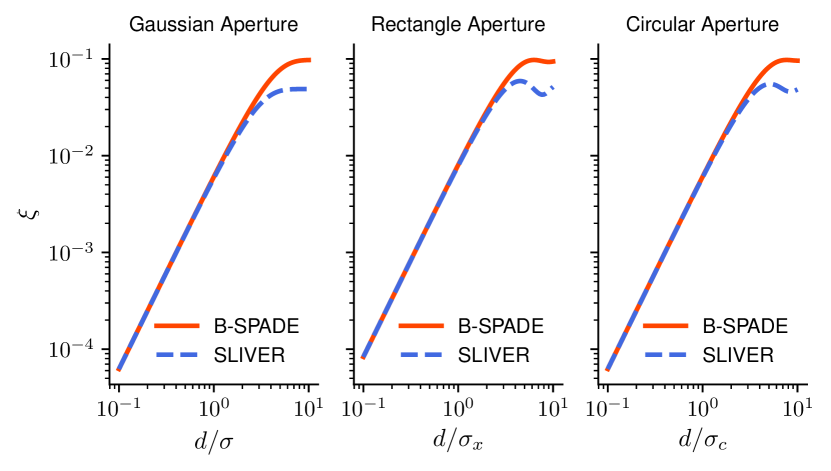
Figure 2: Chernoff exponents for the B-SPADE and SLIVER measurements as a function of the separation $d$. The quantum Chernoff exponent always equals the Chernoff exponent for the B-SPADE measurement. Here, the total strength $\epsilon$ of the thermal sources is set to be $0.1$.

Weak-source model. To compare the performance of B-SPADE and SLIVER with that of direct imaging, we introduce the weak-source model. In most applications in optical microscopy and astronomy, the source brightness $\epsilon\ll 1$ photons per temporal mode Goo85Statistical ; Tsang2016b ; Gottesman2012 ; Tsang2011 . Then, $\rho_{1}$ and $\rho_{2}$ may be considered with high accuracy to be confined to the subspace consisting of zero or one photons, i.e.,

$$\rho_{i}\simeq(1-\epsilon)\left|{\rm vac}\right\rangle\langle{\rm vac}|+\epsilon\eta_{i}$$ (11)

for $i=1,2$, where $\left|{\rm vac}\right\rangle$ denotes the vacuum state and $\eta_{i}$ are the corresponding one-photon states obtained by neglecting $O(\epsilon^{2})$ terms. This approximation enables us to simplify the theory in comparison with Ref. Helstrom1973 and still obtain similar results. The one-photon state for two hypothetical sources can be expressed as

$$\eta(d) =\frac{\left|{\Psi(d/2)}\right\rangle\langle{\Psi(d/2)}|}{2}+\frac{\left|{\Psi(-d/2)}\right\rangle\langle{\Psi(-d/2)}|}{2},$$

$$\left|{\Psi(x^{\prime})}\right\rangle \equiv\int_{\mathcal{I}}{\rm d}x{\rm d}y\,\psi(x-x^{\prime},y)\left|{x,y}\right\rangle,$$ (12)

where we have introduced the one-photon Dirac kets $\left|{x,y}\right\rangle$ satisfying $\langle{x,y}|{x^{\prime},y^{\prime}}\rangle=\delta(x-x^{\prime})\delta(y-y^{\prime})$ and $\int_{\mathcal{I}}{\rm d}x{\rm d}y\left|{x,y}\right\rangle\langle{x,y}|=\openone_{1}$, the identity on the one-photon subspace in the image plane field Tsang2016b . We then have $\eta_{1}=\eta(0)$ and $\eta_{2}=\eta(d)$.

For the specific cases of rectangular and circular hard apertures, Helstrom has derived expressions for the minimum error probability for thermal light sources Helstrom1973 . However, these expressions are very complex. Our weak-source model allows us to simplify the minimum error probability as

$$P_{\mathrm{e,\min}} =\sum_{L=0}^{M}\binom{M}{L}(1-\epsilon)^{M-L}\epsilon^{L}P_{\mathrm{e,\min}|L},$$ (13)

$$P_{\mathrm{e,\min}|L} \equiv\frac{1}{2}-\frac{1}{2}\|p_{2}\eta_{2}^{\otimes L}-p_{1}\eta_{1}^{\otimes L}\|_{1}.$$ (14)

Here, $\binom{M}{L}(1-\epsilon)^{M-L}\epsilon^{L}$ is the probability of $L$ photons arriving at the imaging plane and $P_{\mathrm{e,\min}|L}$ is the minimum probability of error conditioned on detecting $L$ photons in the image plane. The form of equation (13) is due to the fact that the distinguishability between $\rho_{1}$ and $\rho_{2}$ lies in the one-photon sector and the zero-photon event is uninformative. It is implicitly assumed in equation (13) that the source flux is low enough that the on-off detectors’ recovery time is short compared to the average interarrival time of the photons. Either the conditional error probability of equation (14) or the unconditional one of equation (13) can be used as a figure of merit, depending on whether or not the number of the photons arriving at the image plane is measured. Helstrom in Ref. Helstrom1973 took the latter approach, and the performance was studied with respect to the average total number of photons $N=M\epsilon$ detected over the observation interval. On the other hand, in fluorescence microscopy it is common practice to compare the performance of imaging schemes for the same number of detected photons $L$ Ram2006 ; Chao2016 .

We can define a conditional Chernoff exponent $\xi^{\rm(meas)}_{\rm c}$ satisfying $P_{\mathrm{e,\min}|L}^{\rm(meas)}\sim\exp(-L\xi^{\rm(meas)}_{\rm c})$, which is given by equation (3) with $\Lambda_{j}(z)$ replaced by the probability of measurement outcomes conditioned on a photon being detected, i.e., $\Lambda_{j}(z)=\operatorname{Tr}[E(z)\eta_{j}]$. Similarly, the optimum conditional error probability $P_{\mathrm{e,\min}|L}$ decays exponentially with $L$ multiplied by the conditional quantum Chernoff exponent given by $\xi_{\rm c}\equiv-\log\min_{0\leq s\leq 1}\operatorname{Tr}(\eta_{1}^{s}\eta_{2}^{1-s})$. It follows from equation (13) that the (unconditional) Chernoff exponents can be obtained via the relation $e^{-\xi}=1-\epsilon+\epsilon e^{-\xi_{\rm c}}$ and $e^{-\xi^{\rm(meas)}}=1-\epsilon+\epsilon e^{-\xi_{\rm c}^{\rm(meas)}}$. This implies that the (unconditional) Chernoff exponent is monotonically increasing with the conditional one. Particularly, we have $\xi^{\rm meas}\simeq\epsilon\xi_{\rm c}^{\rm meas}$ when $\xi^{\rm meas}\ll 1$. Therefore, we can use either $\xi^{\rm meas}$ or $\xi_{\rm c}^{\rm meas}$ to compare the performance of quantum measurements.

The conditional Chernoff exponents are readily calculated in the weak-source model using equations (12):

$$\xi_{\rm c}^{\rm(B-SPADE)} =\xi_{\rm c}=-2\log\delta(d/2),$$ (15)

$$\xi_{\rm c}^{\rm(SLIVER)} =-\log\frac{1+\delta(d)}{2}.$$ (16)

Note that as $d$ decreases, the SLIVER result converges to the B-SPADE result, which can also be seen in Fig. 2.

Direct Imaging. Direct imaging (DI) using a charge-coupled device (CCD) camera is a standard detection technique in microscopy and telescopy Chao2016 . To compare our schemes to direct imaging, we make the conservative assumption of an ideal noiseless photodetector with infinite spatial resolution and unity quantum efficiency placed in the image plane. In the weak-source model, and conditional on a photon being detected in a given temporal mode, the observation consists of its position of arrival $(x,y)\in\mathcal{I}$. Using equations (12), the resulting probability densities for the observation are $\Lambda_{1}(x,y)=\Upsilon(x,y;0)$ and $\Lambda_{2}(x,y)=\Upsilon(x,y;d)$ under $\textsf{H}_{1}$ and $\textsf{H}_{2}$, respectively, where

$$\Upsilon(x,y;d) \equiv\frac{\left|\psi(x-d/2,y)\right|^{2}}{2}+\frac{\left|\psi(x+d/2,y)\right|^{2}}{2}.$$ (17)

We show in the Methods that the conditional Chernoff exponent for ideal DI in the weak source model scales as $d^{4}$ in the interesting regime of small $d$:

$$\xi^{\rm(DI)}_{\rm c}\simeq\frac{d^{4}}{32}\int_{\mathcal{I}^{\prime}}{\rm d}x{\rm d}y\,\frac{1}{\Upsilon(x,y;0)}\left[\Upsilon^{(2)}(x,y;0)\right]^{2},$$ (18)

where $\Upsilon^{(n)}(x,y;d)$ denotes the $n$-th order partial derivative of $\Upsilon(x,y;d)$ with respect to $d$, and $\mathcal{I}^{\prime}\equiv\{(x,y)\mid\Upsilon(x,y;0)>0\}$. In contrast, the conditional Chernoff exponents of B-SPADE and SLIVER in the weak-source model are of order $d^{2}$, which can be seen by using equation (15)–(16) and $\partial\delta(d)/\partial d|_{d=0}=0$.

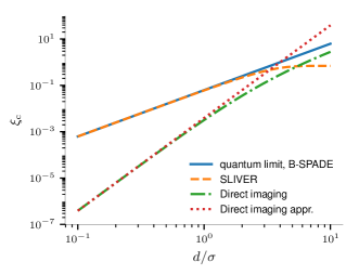
Figure 3: Conditional Chernoff exponents in the weak-source model as functions of the normalized two-source separation $d$ for the Gaussian PSF of equation (9). The Chernoff exponent for B-SPADE (solid) achieves the quantum limit for all values of $d$, while the Chernoff exponent for SLIVER (dashed) is near-quantum-optimal for sub-Rayleigh separations. In this regime, both schemes outperform direct imaging — whose Chernoff exponent is calculated numerically (dash-dotted) as well as by using the small-separation approximation (dotted) given by equation (18) — by more than an order of magnitude.

Table 1: Conditional Chernoff exponents for the Gaussian PSF.

Scheme	Chernoff exponent
B-SPADE/Quantum limit	$d^{2}/16$
SLIVER	$d^{2}/16-d^{4}/512+O(d^{6})$
Direct imaging	$d^{4}/256+O(d^{6})$

The conditional Chernoff exponents for different measurements in the case of the Gaussian PSF are given in Table 1. Here, we have used a Taylor series expansion of equation (16) in $d$ for SLIVER, and used equation (18) for estimating the Chernoff exponent for direct imaging. The characteristic scalings with respect to $d$ of the conditional quantum Chernoff exponent and that of the three measurement schemes are shown in Fig. 3. We see that the Chernoff exponent of SLIVER agrees with the quantum limit for all practical purposes in the sub-Rayleigh regime $d\leq 1$.

Decision rule. In order to choose a hypothesis based on a sequence of B-SPADE/SLIVER observations, we need to fix a decision rule. If the separation $d$ is known, the optimal decision rule is given by the likelihood-ratio test VanTrees2013 : For a given observation record $(z_{1},z_{2},\ldots,z_{M})$, we choose $\mathsf{H}_{2}$ if $\prod_{j=1}^{M}\Lambda_{2}(z_{j})/\Lambda_{1}(z_{j})>p_{1}/p_{2}$, where $p_{1}$ and $p_{2}$ are the prior probabilities of $\mathsf{H}_{1}$ and $\mathsf{H}_{2}$ respectively, and choose $\mathsf{H}_{1}$ otherwise. If the separation is unknown, one can use the generalized-likelihood-ratio test Kay1998 , which first estimates the separation and then does the likelihood-ratio test with the estimated value.

Here, we propose a simplified decision rule that does not require the separation to be known or estimated. Observe that if the detector corresponding to the modes orthogonal to the first mode in the three-mode basis (see equation (23–25) in Methods) clicked for any sample, we can infer with certainty (in either source model) that two point sources are present, i.e., $\mathsf{H}_{2}$ is true. The simplified decision rule is then given by accepting $\mathsf{H}_{1}$ only if this detector does not click during the entire observation period.

From Table 2 in the Methods, under the simplified decision rule, the false-alarm probability for $M$ samples is clearly $\alpha=0$ for both the B-SPADE and SLIVER measurement. The miss error probability is the probability that the detector corresponding to $\mathsf{H}_{2}$ does not click, i.e.,

$$\beta=[\Lambda_{2}\textsf{(off, off)}+\Lambda_{2}\textsf{(on, off)}]^{M},$$ (19)

where $\Lambda_{2}(\cdot,\cdot)$ is the probability of the measurement outcome under $\mathsf{H}_{2}$. It then can shown that $\beta^{\rm(meas)}=\exp(-M\xi^{\rm(meas)})$ for both the B-SPADE and SLIVER measurement.

Discussion. We have examined the problem of discriminating one thermal source from two closely separated ones for a given diffraction-limited imaging system. Using the exact thermal state of the image-plane field, we have derived the quantum Chernoff exponent for the detection problem. We also have used the weak-source model of the image-plane field, which is very accurate in the optical regime due to the low brightness of a thermal source in each temporal mode, to obtain simple expressions for the Chernoff exponent. The per-sample B-SPADE measurement that separates light in the PSF mode from the rest of the field was shown to attain the quantum-optimal Chernoff exponent for all values of two-source separation. Remarkably, it does so without the need for prior knowledge of the value of $d$, joint measurement over multiple modes, or photon-number resolution in each mode. These properties are not shared by the quantum-optimal measurement elucidated by Helstrom Helstrom1973 , which is not a structured receiver. These advantages also adhere to the SLIVER measurement, which is near-quantum-optimal in the sub-Rayleigh regime. Moreover, the experimental design of SLIVER is independent of the particular (reflection-symmetric) PSF of the imaging system.

In fact, the simplified decision rules proposed here for B-SPADE and SLIVER do not require resolving the arrival time of the detected photon or photons. To wit, only a single on-off detector without temporal resolution placed in the output corresponding to the modes orthogonal to the PSF (for B-SPADE) or to the antisymmetric component (for SLIVER) is sufficient for achieving the error probability behavior derived here. Hypothesis $\mathsf{H}_{2}$ is accepted if and only if this detector clicks at any time during the observation period. If we need to simultaneously know the conditional error probability, then at least two photon-number-resolving detectors (or gated on-off detectors with sufficient temporal resolution) are required such that the total number of the photons arriving on the image plane can be obtained from the observation.

Some implementation imperfections that can result in suboptimal performance deserve to be mentioned here. We have so far assumed in our analysis that the optical axes of the B-SPADE and SLIVER devices are perfectly aligned to the source centroids. In practice, we can use a portion of light to estimate the centroid before aligning the B-SPADE/SLIVER devices Tsang2016b ; Nair2016 . From quantum parameter estimation theory, it is known that direct imaging can be used to achieve a good estimate of the centroid, provided that a sufficient number of photons had been collected Tsang2016b . Remarkably, as long as the optical axes are perfectly aligned, the Chernoff exponents of both B-SPADE and SLIVER as well as the quantum limit are insensitive to the relative brightnesses under the weak source model, meaning that the advantage of B-SPADE and SLIVER over direct imaging still holds when the two hypothetical sources do not have equal brightness components. Another possible source of imperfection is dark counts in the photodetectors; this may affect the performance the B-SPADE and SLIVER schemes, especially those using the simplified decision rules. To improve the robustness against dark counts or extraneous background light, we may use feedback strategies, like those developed in the context of distinguishing between optical coherent states Dolinar1973 ; Geremia2004 . These issues will be addressed in subsequent work.

Although sophisticated optical microscopy techniques can help resolve multiple sources better than direct imaging WS15 , the manipulation of the source emission that they require is impossible in astronomical imaging for which the dominant detection technique is direct imaging. Our proof that the linear-optics schemes proposed here can yield Chernoff exponents that are orders of magnitude larger than that of direct imaging, coupled with the rapid recent experimental progress on similar schemes Tang2016 ; Yang2016 ; Tham2017 ; Paur2016 , holds out great promise for applications in astronomy and molecular imaging analysis in the near future.

Methods

Density operators. To calculate the Chernoff exponent and error probabilities, we need to express the density operators $\rho_{1}$ and $\rho_{2}$ in an appropriate basis. We focus on a single temporal mode $\chi(t)$ of the image-plane field satisfying $\int_{0}^{T}\left|\chi(t)\right|^{2}{\rm d}t=1$ on the observation interval $[0,T]$. The two mutually incoherent sources at $\pm\mathbf{d}/2$ under $\textsf{H}_{2}$ are described by statistically independent zero-mean circular complex Gaussian amplitudes $A_{1}$ and $A_{2}$ with the probability density

$$\Pr(A_{1},A_{2})=\prod_{j=1}^{2}\frac{1}{\pi\epsilon_{j}}\exp\left(-\left|A_{j}\right|^{2}/\epsilon_{j}\right),$$ (20)

where $\epsilon_{1}$ and $\epsilon_{2}$ are the brightnesses of the two point sources. The image-plane field conditioned on $(A_{1},A_{2})$ is described quantum-mechanically as a coherent-state, i.e., an eigenstate $\left|{\phi_{A_{1},A_{2}}}\right\rangle$ of the positive-frequency field operator $\hat{E}^{(+)}(\mathbf{r},t)$ in the image plane: $\hat{E}^{(+)}(\mathbf{r},t)\left|{\phi_{A_{1},A_{2}}}\right\rangle=\mathcal{E}_{A_{1},A_{2}}(\mathbf{r})\chi(t)\left|{\phi_{A_{1},A_{2}}}\right\rangle$, where $\mathcal{E}_{A_{1},A_{2}}(\mathbf{r})$ is given by

$$\mathcal{E}_{A_{1},A_{2}}(\mathbf{r})=A_{1}\psi\left(\mathbf{r}-\mathbf{d}/2\right)+A_{2}\psi\left(\mathbf{r}+\mathbf{d}/2\right)$$ (21)

and $\psi(\mathbf{r})$ is the normalized PSF. The density operator under $\mathsf{H}_{2}$ is formally given by

$$\rho_{2} =\int_{\mathbb{C}^{2}}{\rm d}^{2}A_{1}{\rm d}^{2}A_{2}\;\Pr(A_{1},A_{2})\left|{\phi_{A_{1},A_{2}}}\right\rangle\langle{\phi_{A_{1},A_{2}}}|.$$ (22)

Note that $\rho_{2}$ depends on the separation $d$ and is reduced to $\rho_{1}$ when setting $d=0$. Moreover, it can be seen from equation (21) that under $\mathsf{H}_{1}$ we have $\mathcal{E}_{A_{1},A_{2}}(\mathbf{r})=(A_{1}+A_{2})\psi(\mathbf{r})$. Thus, it is evident that, while the relevant coherent states are defined on a complete set of transverse-spatial modes on $\mathcal{I}$, only three orthonormal modes are in excited (non-vacuum) states. These may be chosen as

$$\phi_{1}(\mathbf{r}) =\psi(\mathbf{r}),$$ (23)

$$\phi_{2}(\mathbf{r}) =\frac{1}{\sqrt{1-\mu^{2}}}\left[\frac{\psi(\mathbf{r}-\mathbf{d}/2)+\psi(\mathbf{r}+\mathbf{d}/2)}{2\sqrt{\lambda_{+}}}-\mu\,\psi(\mathbf{r})\right],$$ (24)

$$\phi_{3}(\mathbf{r}) =\frac{\psi(\mathbf{r}-\mathbf{d}/2)-\psi(\mathbf{r}+\mathbf{d}/2)}{2\sqrt{\lambda_{-}}},$$ (25)

where $\lambda_{\pm}\equiv(1\pm\delta(d))/2$ and $\mu$ is given by equation (7). Using $\{\phi_{1}(\mathbf{r}),\phi_{2}(\mathbf{r}),\phi_{3}(\mathbf{r})\}$ as a spatial-mode basis, we have

$$\mathcal{E}_{A_{1},A_{2}}(\mathbf{r})=A_{+}\left[\mu\phi_{1}(\mathbf{r})+\sqrt{1-\mu^{2}}\phi_{2}(\mathbf{r})\right]+A_{-}\phi_{3}(\mathbf{r}),$$ (26)

where $A_{+}=\sqrt{\lambda_{+}}(A_{1}+A_{2})$ and $A_{-}=\sqrt{\lambda_{-}}(A_{1}-A_{2})$ are two circular complex Gaussian amplitudes random variables. When $\epsilon_{1}=\epsilon_{2}=\epsilon/2$, the random variables $A_{+}$ and $A_{-}$ are statistically independent Nair2016 . In such a case, we get

$$\rho_{1} =\rho_{\textsf{th}}\left(\epsilon\right)\otimes\left|{0}\right\rangle\langle{0}|\otimes\left|{0}\right\rangle\langle{0}|,$$ (27)

$$\rho_{2} =U\left[\rho_{\textsf{th}}(\epsilon_{+})\otimes\left|{0}\right\rangle\langle{0}|\right]U^{{\dagger}}\otimes\rho_{\textsf{th}}(\epsilon_{-}),$$ (28)

where $\rho_{\textsf{th}}(\epsilon)=\sum_{n}[\epsilon^{n}/(\epsilon+1)^{n+1}]\left|{n}\right\rangle\langle{n}|$ is the single-mode thermal state with $\epsilon$ average photons MW95 ; Shapiro2009 , $U$ is a unitary beamsplitter transformation with transmissivity $\mu$ acting on the first two modes. The $d$-dependent quantities $\epsilon_{\pm}$ and $\mu$ are given by equation (7). The transmissivity $\mu$ takes values in the range [-1,1] and equals unit when $d=0$. The beamsplitter implements the transformation

$$U\left|{\alpha}\right\rangle\otimes\left|{\beta}\right\rangle=|\mu\alpha-\sqrt{1-\mu^{2}}\beta\rangle\otimes|\mu\beta+\sqrt{1-\mu^{2}}\alpha\rangle$$ (29)

for input coherent states $\left|{\alpha}\right\rangle$ and $\left|{\beta}\right\rangle$, while for a number state-vacuum input $\left|{n}\right\rangle\left|{0}\right\rangle$, we have

$$U\left|{n}\right\rangle\otimes\left|{0}\right\rangle=\sum_{k=0}^{n}\sqrt{\binom{n}{k}}\,\mu^{k}\,(1-\mu^{2})^{\frac{n-k}{2}}\left|{k,n-k}\right\rangle.$$ (30)

Quantum Chernoff exponent. The quantum Chernoff exponent is given by $\xi=-\log\min_{0\leq s\leq 1}Q_{s}$ with $Q_{s}\equiv\operatorname{Tr}(\rho_{1}^{s}\rho_{2}^{1-s})$. Using equations (27), (28), and (30), we get after some algebra:

$$Q_{s} =\frac{1}{ap^{s}(1-bq^{s})},$$ (31)

where the coefficients are

$$\begin{split}a&=(1+\epsilon_{+})(1+\epsilon_{-}),\quad b=\frac{\epsilon_{+}}{1+\epsilon_{+}}\mu^{2},\\ p&=\frac{1+\epsilon}{(1+\epsilon_{+})(1+\epsilon_{-})},\quad q=\frac{\epsilon(1+\epsilon_{+})}{\epsilon_{+}(1+\epsilon)}.\end{split}$$ (32)

It follows from $0\leq\epsilon_{\pm}\leq\epsilon$ and $\epsilon_{+}+\epsilon_{-}=\epsilon$ that $p\leq 1$ and $q\geq 1$. Thus, $Q_{s}$ takes its minimum at $s=0$, i.e.,

$$\min_{0\leq s\leq 1}Q_{s} =Q_{0}=\frac{1}{(1+\epsilon_{-})(1+\epsilon_{+}-\mu^{2}\epsilon_{+})},$$ (33)

from which we obtain the quantum Chernoff exponent in equation (5).

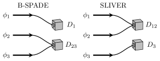
Figure 4: Effective description of the B-SPADE and SLIVER measurements in the three-mode basis. Here, $\phi_{1}$, $\phi_{2}$ and $\phi_{3}$ are the three orthonormal modes of equations (23)-(25) used to represent the density operators in equation (27) and (28).

Table 2: Probability distributions of single-sample outcomes for the two on-off detectors used in the B-SPADE and SLIVER measurement. The first entry in each outcome refers to detection of the filtered PSF mode for B-SPADE and the symmetric field for SLIVER. The probability represented by $*$ can be obtained by the normalization of the probability distribution.

Measurement	Hypothesis	Probability of Event
		(off, off)	(on, off)	(off, on)	(on, on)
B-SPADE	$\mathsf{H}_{1}$	$\frac{1}{1+\epsilon}$	$\frac{\epsilon}{1+\epsilon}$	0	0
	$\mathsf{H}_{2}$	$\frac{1}{(1+\epsilon_{+})(1+\epsilon_{-})}$	$\frac{\mu^{2}\epsilon_{+}}{(1+\epsilon_{+})(1+\epsilon_{-})(1+\epsilon_{+}-\mu^{2}\epsilon_{+})}$	$\frac{1}{1+\mu^{2}\epsilon_{+}}-\frac{1}{(1+\epsilon_{+})(1+\epsilon_{-})}$	$*$
SLIVER	$\mathsf{H}_{1}$	$\frac{1}{1+\epsilon}$	$\frac{\epsilon}{1+\epsilon}$	0	0
	$\mathsf{H}_{2}$	$\frac{1}{(1+\epsilon_{+})(1+\epsilon_{-})}$	$\frac{\epsilon_{+}}{(1+\epsilon_{+})(1+\epsilon_{-})}$	$\frac{\epsilon_{-}}{(1+\epsilon_{+})(1+\epsilon_{-})}$	$\frac{\epsilon_{+}\epsilon_{-}}{(1+\epsilon_{+})(1+\epsilon_{-})}$

B-SPADE and SLIVER. To calculate the Chernoff exponents as well as the error probabilities for B-SPADE and SLIVER, it will be convenient to only focus on the effective action of the measurement on the relevant Hilbert subspace. Figure 4 illustrates the effective actions of B-SPADE and SLIVER on the mode subspace spanned by $\phi_{1}(\mathbf{r})$, $\phi_{2}(\mathbf{r})$ and $\phi_{3}(\mathbf{r})$. The B-SPADE measurement discriminates the first mode from the other two, while the SLIVER measurement discriminates the first two modes from the third, which is the sole excited antisymmetric mode. We emphasize that our schemes are very different from a detector that resolves each of the modes $\phi_{1}(\mathbf{r})$, $\phi_{2}(\mathbf{r})$ and $\phi_{3}(\mathbf{r})$, since implementing such a detector would require knowledge of $d$. Our schemes, on the other hand, work for any $d$. Using equations (27) and (28) and the effective action of the measurements shown in Fig. 4, the probability distribution of measurement outcomes can be easily obtained as given in Table 2, on which the calculation of the Chernoff exponents is based.

For B-SPADE, we get

$$Q_{s}^{\rm(B-SPADE)}=\frac{1+\tilde{b}\tilde{q}^{s}}{ap^{s}},$$ (34)

where $a$ and $p$ are given in equation (32), $\tilde{b}=\mu^{2}\epsilon_{+}/(1+\epsilon_{+}-\mu^{2}\epsilon_{+})$, and $\tilde{q}=\epsilon(1+\epsilon_{+}-\mu^{2}\epsilon_{+})/\mu^{2}\epsilon_{+}\geq 1$. It follows that $Q_{s}$ is minimized over $[0,1]$ by taking $s=0$, leading to the result of $\xi^{\rm(B-SPADE)}$ in equation (5). In the weak-source model, the probability distribution of a detected photon being at the two output ports is $\{1,0\}$ under $\mathsf{H}_{1}$ and $\{\delta(d/2)^{2},1-\delta(d/2)^{2}\}$ under $\mathsf{H}_{2}$. Thus, one can easily obtain the result of $\xi_{\rm c}^{\rm(B-SPADE)}$ as shown in equation (15).

For SLIVER, the structure of $\rho_{1}$ and $\rho_{2}$ implies that the two detectors fire independently under both hypotheses. From these equations, the Chernoff exponent of SLIVER can be calculated (and corresponds to $s=0$ as for B-SPADE) with the result of equation (6). In the weak source model, the probability distribution of a detected photon being at the two output ports is $\{1,0\}$ under $\mathsf{H}_{1}$ and $\{[\delta(d)+1]/2,[1-\delta(d)]/2\}$ under $\mathsf{H}_{2}$. Thus, one can easily obtain the result of $\xi_{\rm c}^{\rm(SLIVER)}$ as shown in equation (16).

Leading term of Chernoff exponent. For a given measurement scheme, let $\Upsilon(z;d)$ be the resulting probability density of a measurement outcome $z$, where $d$ is the distance between the two hypothetic point sources. The Chernoff exponent of equation (3) for testing $\mathsf{H}_{2}$ ($d>0$) against $\mathsf{H}_{1}$ ($d=0$) can be written as $\xi(d)=-\log\min_{0\leq s\leq 1}Q_{s}(d)$ with $Q_{s}(d)\equiv\int\mathrm{d}\mu(z)\Upsilon(z;0)^{1-s}\Upsilon(z;d)^{s}$. Let us now focus on the leading term of $\xi(d)$ for small separations $d\approx 0$, where the optimal measurement performs much better than direct imaging. We expand $Q_{s}(d)$ in a Taylor series as

$$Q_{s}(d) =1+\sum_{k=1}^{\infty}\frac{d^{k}}{k!}Q_{s,k},$$ (35)

$$Q_{s,k} \equiv\int_{\Omega}{\rm d}\mu(z)\,\Upsilon(z;0)^{1-s}\left.\frac{\partial^{k}\Upsilon(z;d)^{s}}{\partial d^{k}}\right|_{d=0},$$ (36)

where $\Omega\equiv\{z\mid\Upsilon(z;0)>0\}$. These coefficients $Q_{s,k}$ are independent of $d$. Although in our model the separation $d$ is nonnegative, the PSFs in equation (9) can be easily extended to real numbers and meanwhile assured to be smooth at $d=0$. It then follows from equation (12) that $\Upsilon(z;d)=\Upsilon(z;-d)$ and thus all odd derivatives of $\Upsilon(z;d)$ with respect to $d$ at $d=0$ vanish for an arbitrary $z$. As a result, we have

$$\begin{split}Q_{s,1}&=Q_{s,3}=0,\quad Q_{s,2}=sg^{(2)}(0),\\ Q_{s,4}&=3s(s-1)\mathcal{K}+sg^{(4)}(0),\end{split}$$ (37)

where $g^{(k)}$ denotes the $k$-th derivatives of $g(d)\equiv\int_{\Omega}{\rm d}\mu(z)\,\Upsilon(z;d)$ and

$$\mathcal{K}\equiv\int_{\Omega}{\rm d}\mu(z)\,\frac{1}{\Upsilon(z;0)}\left[\frac{\partial^{2}\Upsilon(z;d)}{\partial d^{2}}\right]_{d=0}^{2}.$$ (38)

For the ideal direct imaging scenario in the weak-source model, the measurement outcome $z$ is the coordinates of a detected photon in the image plane, i.e., $z=(x,y)\in\mathcal{I}$. Suppose that the two point sources are aligned along the $x$-axis, $\Upsilon(z;d)$ is then given by equation (17) with $z=(x,y)$. For all three typical kinds of PSFs considered in this work, we have $g(d)=1$ for direct imaging. In such a case, the leading $d$-dependent term in the Taylor series of $Q_{s}(d)$ is of fourth order. It then follows that $\xi_{\rm c}^{\rm(DI)}\simeq\frac{d^{4}}{32}\mathcal{K}$, which is equation (18). On the other hand, for B-SPADE and SLIVER, it can be seen from Table 2 that $g(d)=\Lambda_{2}(\textsf{off,off})+\Lambda_{2}(\textsf{on,off})$, so that $g^{(2)}(0)$ is nonzero and the leading term in $Q_{s}(d)$ is second-order in $d$.

Acknowledgments
We thank Mankei Tsang for several useful discussions. This work was supported by the Singapore National Research Foundation under NRF Grant No. NRF-NRFF2011-07, the Singapore Ministry of Education Academic Research Fund Tier 1 Project R-263-000-C06-112, the Natural Science Foundation of Zhejiang Province of China under Grant No. LY18A050003, the Defense Advanced Research Projects Agency’s (DARPA) Information in a Photon (InPho) program under Contract No. HR0011-10-C-0159, the REVEAL and EXTREME Imaging program, and the Air Force Office of Scientific Research under Grant No. FA9550-14-1-0052.

Author contributions
X.-M. L. performed the weak-source model analysis. H. K., S. G., J. H. S., and R. N. performed the thermal-state analysis. R. N. performed the SLIVER analyses. X.-M. L. and R. N. wrote the manuscript. All the authors discussed extensively during the course of this work. This paper extends and unifies preliminary work in the preprints Krovi2016 (thermal-state model) and Lu2016 (weak-source model).

Competing financial interests: The authors declare no competing financial interests.

References

- (1) Lord Rayleigh, F. R. S. Xxxi. investigations in optics, with special reference to the spectroscope. Philosophical Magazine Series 5 8, 261–274 (1879).
- (2) Feynman, R., Leighton, R. & Sands, M. The Feynman Lectures on Physics:Volume I (Addison-Wesley, 1963).
- (3) Ram, S., Ward, E. S. & Ober, R. J. Beyond Rayleigh’s criterion: A resolution measure with application to single-molecule microscopy. Proc. Natl. Acad. Sci. U.S.A. 103, 4457–4462 (2006).
- (4) Chao, J., Ward, E. S. & Ober, R. J. Fisher information theory for parameter estimation in single molecule microscopy: tutorial. J. Opt. Soc. Am. A 33, B36–B57 (2016).
- (5) Helstrom, C. W. Quantum Detection and Estimation Theory (Academic Press, New York, 1976).
- (6) Holevo, A. S. Probabilistic and Statistical Aspects of Quantum Theory (North-Holland, Amsterdam, 1982).
- (7) Tsang, M., Nair, R. & Lu, X.-M. Quantum theory of superresolution for two incoherent optical point sources. Phys. Rev. X 6, 031033 (2016).
- (8) Nair, R. & Tsang, M. Interferometric superlocalization of two incoherent optical point sources. Opt. Express 24, 3684–3701 (2016).
- (9) Tsang, M., Nair, R. & Lu, X.-M. Semiclassical theory of superresolution for two incoherent optical point sources (2016). eprint 1602.04655.
- (10) Nair, R. & Tsang, M. Far-field superresolution of thermal electromagnetic sources at the quantum limit. Phys. Rev. Lett. 117, 190801 (2016).
- (11) Ang, S. Z., Nair, R. & Tsang, M. Quantum limit for two-dimensional resolution of two incoherent optical point sources. Phys. Rev. A 95, 063847 (2017).
- (12) Lupo, C. & Pirandola, S. Ultimate precision bound of quantum and subwavelength imaging. Phys. Rev. Lett. 117, 190802 (2016).
- (13) Rehacek, J. et al. Dispelling Rayleigh’s curse eprint 1607.05837.
- (14) Tsang, M. Subdiffraction incoherent optical imaging via spatial-mode demultiplexing. New Journal of Physics 19, 023054 (2017).
- (15) Kerviche, R., Guha, S. & Ashok, A. Fundamental limit of resolving two point sources limited by an arbitrary point spread function. In 2017 IEEE International Symposium on Information Theory (ISIT), 441–445 (2017).
- (16) Yang, F., Nair, R., Tsang, M., Simon, C. & Lvovsky, A. I. Fisher information for far-field linear optical superresolution via homodyne or heterodyne detection in a higher-order local oscillator mode. Phys. Rev. A 96, 063829 (2017).
- (17) Tang, Z. S., Durak, K. & Ling, A. Fault-tolerant and finite-error localization for point emitters within the diffraction limit. Opt. Express 24, 22004–22012 (2016).
- (18) Yang, F., Nair, R., Tsang, M., Simon, C. & Lvovsky, A. I. Fisher information for far-field linear optical superresolution via homodyne or heterodyne detection in a higher-order local oscillator mode. Phys. Rev. A 96, 063829 (2017).
- (19) Tham, W.-K., Ferretti, H. & Steinberg, A. M. Beating Rayleigh’s curse by imaging using phase information. Phys. Rev. Lett. 118, 070801 (2017).
- (20) Paúr, M., Stoklasa, B., Hradil, Z., Sánchez-Soto, L. L. & Rehacek, J. Achieving the ultimate optical resolution. Optica 3, 1144–1147 (2016).
- (21) Harris, J. L. Resolving power and decision theory. J. Opt. Soc. Am. 54, 606–611 (1964).
- (22) Helstrom, C. Resolution of point sources of light as analyzed by quantum detection theory. IEEE Trans. Inform. Theory 19, 389–398 (1973).
- (23) Acuna, C. O. & Horowitz, J. A statistical approach to the resolution of point sources. J. Appl. Statist. 24, 421–436 (1997).
- (24) Shahram, M. & Milanfar, P. Statistical and information-theoretic analysis of resolution in imaging. IEEE Trans. Inform. Theor. 52, 3411–3437 (2006).
- (25) Dutton, Z., Shapiro, J. H. & Guha, S. Ladar resolution improvement using receivers enhanced with squeezed-vacuum injection and phase-sensitive amplification. J. Opt. Soc. Am. B 27, A63–A72 (2010).
- (26) Labeyrie, A., Lipson, S. G. & Nisenson, P. An Introduction to Optical Stellar Interferometry (Cambridge University Press, 2006).
- (27) Nan, X. et al. Single-molecule superresolution imaging allows quantitative analysis of raf multimer formation and signaling. Proc. Natl. Acad. Sci. U.S.A. 110, 18519–18524 (2013).
- (28) Hayashi, M. Quantum Information: An Introduction (Springer-Verlag, Berlin Heidelberg, 2006), 1 edn.
- (29) Holevo, A. Statistical decision theory for quantum systems. J. Multivar. Anal. 3, 337 – 394 (1973).
- (30) Reck, M., Zeilinger, A., Bernstein, H. J. & Bertani, P. Experimental realization of any discrete unitary operator. Phys. Rev. Lett. 73, 58–61 (1994).
- (31) Morizur, J.-F. et al. Programmable unitary spatial mode manipulation. J. Opt. Soc. Am. A 27, 2524–2531 (2010).
- (32) Miller, D. A. B. Reconfigurable add-drop multiplexer for spatial modes. Opt. Express 21, 20220–20229 (2013).
- (33) Chernoff, H. A measure of asymptotic efficiency for tests of a hypothesis based on the sum of observations. Ann. Math. Statist. 23, 493–507 (1952).
- (34) Van Trees, H. L., Bell, K. L. & Tian, Z. Detection, Estimation, and Modulation Theory, Part I (Wiley, 2013), 2nd edition edn.
- (35) Cover, T. & Thomas, J. Elements of Information Theory (Wiley, 2006), 2nd edition edn.
- (36) Ogawa, T. & Hayashi, M. On error exponents in quantum hypothesis testing. IEEE Transactions on Information Theory 50, 1368–1372 (2004).
- (37) Kargin, V. On the Chernoff bound for efficiency of quantum hypothesis testing. Ann. Stat. 33, 959–976 (2005).
- (38) Audenaert, K. M. R. et al. Discriminating states: The quantum Chernoff bound. Phys. Rev. Lett. 98, 160501 (2007).
- (39) Nussbaum, M. & Szkoła, A. The Chernoff lower bound for symmetric quantum hypothesis testing. Ann. Statist. 37, 1040–1057 (2009).
- (40) Audenaert, K., Nussbaum, M., Szkoła, A. & Verstraete, F. Asymptotic error rates in quantum hypothesis testing. Commun. Math. Phys. 279, 251–283 (2008).
- (41) Goodman, J. W. Introduction to Fourier Optics (Roberts and Company Publishers, 2005), 3rd edn.
- (42) Goodman, J. W. Statistical Optics (John Wiley & Sons, 1985).
- (43) Gottesman, D., Jennewein, T. & Croke, S. Longer-baseline telescopes using quantum repeaters. Phys. Rev. Lett. 109, 070503 (2012).
- (44) Tsang, M. Quantum nonlocality in weak-thermal-light interferometry. Phys. Rev. Lett. 107, 270402 (2011).
- (45) Kay, S. M. Fundamentals of Statistical Signal Processing, Volume II: Detection Theory (Prentice Hall, New Jersey, 1998), 1st edn.
- (46) Dolinar, S. J. An optimum receiver for the binary coherent state quantum channel. MIT Res. Lab. Electron. Quart. Progr. Rep. 111, 115–120 (1973).
- (47) Geremia, J. Distinguishing between optical coherent states with imperfect detection. Phys. Rev. A 70, 062303 (2004).
- (48) Weisenburger, S. & Sandoghdar, V. Light microscopy: an ongoing contemporary revolution. Contemporary Physics 56, 123–143 (2015).
- (49) Mandel, L. & Wolf, E. Optical Coherence and Quantum Optics (Cambridge University Press, Cambridge, 1995).
- (50) Shapiro, J. H. The quantum theory of optical communications. IEEE Journal of Selected Topics in Quantum Electronics 15, 1547 –1569 (2009).
- (51) Krovi, H., Guha, S. & Shapiro, J. H. Attaining the quantum limit of passive imaging (2016). eprint arXiv:1609.00684.
- (52) Lu, X.-M., Nair, R. & Tsang, M. Quantum-optimal detection of one-versus-two incoherent sources with arbitrary separation (2016). eprint arXiv:1609.03025.