Loop currents and anomalous Hall effect from time-reversal symmetry-breaking superconductivity on the honeycomb lattice

Abstract

We study a tight-binding model on the honeycomb lattice of chiral $d$-wave superconductivity that breaks time-reversal symmetry. Due to its nontrivial sublattice structure, we show that it is possible to construct a gauge-invariant time-reversal-odd bilinear of the pairing potential. The existence of this bilinear reflects the sublattice polarization of the pairing state. We show that it generates persistent loop current correlations around each lattice site and opens a topological mass gap at the Dirac points, resembling Haldane’s model of the anomalous quantum Hall effect. In addition to the usual chiral $d$-wave edge states, there also exist electron-like edge resonances due to the topological mass gap. We show that the presence of loop-current correlations directly leads to a nonzero intrinsic ac Hall conductivity, which produces the polar Kerr effect without an external magnetic field. Similar results also hold for the nearest-neighbor chiral $p$-wave pairing. We briefly discuss the relevance of our results to superconductivity in twisted bilayer graphene.

I Introduction

Chiral superconductors, which possess order parameters that break time-reversal symmetry, are currently the subject of much attention due to their nontrivial topological properties. SatoRPP2017 ; KallinRPP2016 The best known example of a chiral pairing state is the A phase of superfluid ³He. LeggettRMP1975 Here Cooper pairs have the orbital angular momentum quantum numbers $L=1$ and $L_{z}=\pm 1$, and the pairing potential has $(p_{x}\pm ip_{y})$-wave symmetry. A direct solid-state analogue of this phase is believed to be realized in the triplet superconductor $\rm Sr_{2}RuO_{4}$. Mackenzie2017 Chiral superconductivity can also be obtained for pairing with higher-order orbital angular momentum. For example, the low-temperature superconducting phase of $\rm UPt_{3}$ may realize a chiral $f$-wave state, JoyntRMP2002 ; UPt3chiral while chiral $d$-wave superconducting states have been proposed for $\rm URu_{2}Si_{2}$, Kasahara2007 $\rm SrPtAs$, Fischer2014 and twisted bilayer graphene. Cao2018 Many other materials have been predicted to show chiral superconductivity, such as water-intercalated sodium cobaltate Na_xCoO${}_{2}\cdot y$H₂O, NaxCoO2papers the half-Heusler compound $\rm YPtBi$, Bry2016 and transition metal dichalcogenides. TiSe2 ; MoS2 ; dichalcogenides

The breaking of time-reversal symmetry in a chiral superconductor can be revealed by a number of experimental techniques, e.g. muon spin rotation or Josephson interferometry. KallinRPP2016 In the last dozen years, measurements of the polar Kerr effect have emerged as a key experimental probe. KapNJP2009 It gives evidence for an anomalous ac Hall conductivity at zero external magnetic field, which is a signature of broken time-reversal symmetry. A number of superconductors have been shown to display a nonzero Kerr signal below their critical temperatures, specifically Sr₂RuO₄, Sr2RuO4Kerr UPt₃, UPt3Kerr URu₂Si₂, URu2Si2Kerr PrOs₄Sb₁₂, PrOs4Sb12Kerr and Bi/Ni bilayers. BiNiKerr Although these observations give clear evidence for broken time-reversal symmetry, there is ongoing debate over the mechanism underlying the polar Kerr effect in chiral superconductors. An extrinsic Kerr effect may originate from impurity scattering, Goryo2008 ; Lutchyn2009 ; Koenig2017 whereas an intrinsic Kerr effect is possible for clean multiband superconductors. Wysokinski2012 ; Taylor2012 ; GradhandSr2RuO4 ; RobbinsSr2RuO4 ; KomendovaPRL2017 ; KerrUPt3_theory ; JoyntWu2017 ; Triola2017 The latter mechanism requires that the pairing potential depends on electronic degrees of freedom beyond the usual spin index, e.g.  orbital or sublattice indices. However, it remains unclear what general model-independent conditions these additional electronic degrees of freedom have to satisfy in order to produce a Kerr effect. Here we develop a general condition for this and then apply it to a minimal model of a chiral $d$-wave superconductor in order to clarify the underlying physics.

Such a minimal theoretical model of a chiral superconductor is provided by the extended Hubbard model on the honeycomb lattice. Baskaran2002 ; Uchoa2007 Various theoretical techniques BlaSchDon2007 ; Honerkamp2008 ; Pathak2010 ; Raghu2010 ; Ma2011 ; Kiesel2012 ; Nandkishore2012a ; Nandkishore2012b ; Wu2013 ; Gu2013 ; BlaSchPRB2014 ; JiangPRX2014 ; BlaSchHonJPCM2014 ; XiaoEPL2016 ; Xu2016 ; Ying2017 applied to this system generally agree on the existence of a spin-singlet chiral $d$-wave state at a doping level close to the van Hove singularity. Closer to half-filling, however, different methods have yielded singlet and triplet pairings, Raghu2010 ; BlaSchPRB2014 ; Faye2015 ; XiaoEPL2016 ; Xu2016 ; Ying2017 ; RoyJur2014 pair-density-wave Kekule order, Roy2010 ; Kunst2015 or an unconventional coexistence with antiferromagnetism. BlackSchaeffer2015 ; Faye2016 ; QiFuSunGu2017 The purpose of our paper is not to further interrogate the phase diagram, but rather to examine the properties of the chiral $d$-wave state in the case where the nearest-neighbor pairing dominates. Such inter-sublattice pairing would satisfy the multiband requirement Taylor2012 for the anomalous Hall conductivity. Thus, chiral $d$-wave pairing on the honeycomb lattice provides a minimal model of the intrinsic Kerr effect, in contrast to the more complicated multiband models of Sr₂RuO₄ Wysokinski2012 ; Taylor2012 ; GradhandSr2RuO4 ; RobbinsSr2RuO4 ; KomendovaPRL2017 and UPt₃. KerrUPt3_theory ; JoyntWu2017 ; Triola2017 The recent discovery of superconductivity in twisted bilayer graphene, Cao2018 which has been proposed to realize a chiral $d$-wave state, Wu2018 ; Xu2018 ; Fidrysiak2018 ; Guo2018 ; Su2018 ; Liu2018 makes this study timely. We discuss the relationship between our model and these proposals in more detail near the end of the paper.

Using this minimal model as an example, we show how to construct a gauge-invariant time-reversal-odd term by taking the product of the pairing potential and its Hermitian conjugate. The existence of such a bilinear is a prerequisite for the experimental detection of time-reversal symmetry-breaking superconductivity in a clean and homogeneous system. In the honeycomb model, the bilinear arises from the varying participation of the two sublattices in the pairing across the Brillouin zone and describes spontaneous breaking of the discrete $\mathbb{Z}_{2}$ time-reversal symmetry. The presence of this term results in the opening of a topological mass gap at the Dirac points and the emergence of persistent loop current correlations, in a striking analogy to Haldane’s model of the anomalous Hall insulator. Haldane1988 Furthermore, we show that the loop current correlations imply a nonzero anomalous Hall conductivity, hence connecting the polar Kerr effect in superconductors with the time-reversal-odd bilinear product of the pairing potentials.

The paper is organized as follows. We start in Sec. II by introducing the model of spin-singlet chiral $d$-wave pairing on the honeycomb lattice. In Sec. III we define a gauge-invariant bilinear product of the superconducting pairing potentials that breaks time-reversal symmetry. As a consequence of the existence of this bilinear, we demonstrate the opening of the mass gap at the Dirac point in Sec. IV and the existence of loop currents in Sec. V. The anomalous ac Hall conductivity is calculated in Sec. VI. A phenomenological description of the loop currents is outlined in Sec. VII. The relationship of our work to proposals of chiral $d$-wave superconductivity in twisted bilayer graphene is discussed in Sec. VIII. We conclude in Sec. IX with a brief discussion of the broader implications of our work. In Appendix A we present similar results for a spin-triplet chiral $p$-wave state on the honeycomb lattice. In Appendix B we show how the bilinear discussed in Sec. II applies to a broader class of Hamiltonians. More general expressions for the loop-current order and the Hall conductivity in the case of inequivalent sublattices are given in Appendix C. The high-frequency small-gap limit of the ac Hall conductivity is derived in Appendix D.

II Microscopic model

The Bogoliubov-de Gennes (BdG) Hamiltonian of superconducting pairing on the honeycomb lattice is

$$H=\sum_{\bm{k}}\Psi_{\bm{k}}^{\dagger}\left(\begin{array}[]{cc}H_{0}({\bm{k}})&\Delta({\bm{k}})\\ \Delta^{\dagger}({\bm{k}})&-H^{T}_{0}(-{\bm{k}})\end{array}\right)\Psi_{\bm{k}}\,,$$ (1)

where $\Psi_{\bm{k}}=(a_{\bm{k},\uparrow},b_{\bm{k},\uparrow},a^{\dagger}_{-\bm{k},\downarrow},b^{\dagger}_{-\bm{k},\downarrow})^{T}$, and the operator $a_{{\bm{k}},\sigma}$ ($b_{{\bm{k}},\sigma}$) annihilates an electron with momentum ${\bm{k}}=(k_{x},k_{y})$ and spin $\sigma$ on the $A$ ($B$) sublattices. In Eq. (1), $H_{0}(\bm{k})$ and $\Delta(\bm{k})$ are $2\times 2$ matrices in the sublattice space, and the absence of spin-orbit coupling allows the spin variables to be factored out.

Using the Pauli matrices $s_{\lambda}$ to encode the sublattice degree of freedom, we write the normal-state Hamiltonian as

$$H_{0}({\bm{k}})=\epsilon^{x}_{\bm{k}}{s}_{x}+\epsilon^{y}_{\bm{k}}{s}_{y}+\delta_{s}{s}_{z}-\mu{s}_{0},$$ (2)

$$\epsilon^{x}_{\bm{k}}=-t\sum\limits_{j=1}^{3}\cos({\bm{k}}\cdot{\bm{R}}_{j}),\;\;\epsilon^{y}_{\bm{k}}=t\sum\limits_{j=1}^{3}\sin({\bm{k}}\cdot{\bm{R}}_{j}).$$ (3)

Here $\mu$ is the chemical potential, $t$ is the nearest-neighbor hopping amplitude, and the ${\bm{R}}_{j}$ are the vectors of length $a$ connecting an $A$ site to its neighboring $B$ sites, see Fig. 1. For generality, we also include the Semenoff term Semenoff as a staggered potential $\delta_{s}$. This makes the $A$ and $B$ sites inequivalent, hence breaking inversion symmetry and lowering the point group from $D_{6h}$ to $D_{3h}$.

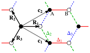
Figure 1: (Color online) Schematic diagram of the chiral $d$-wave pairing on the honeycomb lattice. The two sublattices are denoted by the black ($A$) and white ($B$) circles. The nearest-neighbor vectors ${\bm{R}}_{j=1,2,3}$ are shown as the black arrows, whereas ${\bm{c}}_{1}$ and ${\bm{c}}_{2}$ denote the primitive lattice vectors. The pairing potentials on the three nearest-neighbor bonds are $\{\Delta_{1},\Delta_{2},\Delta_{3}\}=\Delta\{1,e^{2\pi i/3},e^{4\pi i/3}\}$. The time-reversed pairing is obtained by complex conjugation.

We consider chiral spin-singlet superconducting pairing on the nearest-neighbor bonds along the directions ${\bm{R}}_{j}$ shown in Fig. 1. This gives the pairing term

$$\Delta_{\pm}({\bm{k}})=\Delta\sum_{j=1}^{3}e^{\mp i\phi_{j}}\left(\begin{array}[]{cc}0&e^{i{\bm{k}}\cdot{\bm{R}}_{j}}\\ e^{-i{\bm{k}}\cdot{\bm{R}}_{j}}&0\end{array}\right).$$ (4)

The magnitude $\Delta$ of the pairing potential is the same for each bond $j$, but the phase is $\phi_{j}=(j-1)2\pi/3$, and the two choices of sign in Eq. (4) define degenerate pairing potentials with opposite chiralities. A similar chiral spin-triplet pairing is discussed in Appendix A.

The two pairing potentials in Eq. (4) can be written in terms of the Pauli matrices $s_{\lambda}$

$$\Delta_{+}(\bm{k})=\Delta^{x}_{\bm{k}}s_{x}+\Delta^{y}_{\bm{k}}s_{y}\,,$$ (5)

$$\Delta_{-}(\bm{k})=(\Delta^{x}_{\bm{k}})^{*}s_{x}+(\Delta^{y}_{\bm{k}})^{*}s_{y}\,,$$ (6)

where

$$\Delta^{x}_{\bm{k}}=\Delta\sum_{j=1}^{3}e^{-i\phi_{j}}\cos({\bm{k}}\cdot{\bm{R}}_{j})\,,$$ (7)

$$\Delta^{y}_{\bm{k}}=-\Delta\sum_{j=1}^{3}e^{-i\phi_{j}}\sin({\bm{k}}\cdot{\bm{R}}_{j})\,.$$ (8)

The pairing potentials in Eq. (4) can also be expressed in terms of basis states of the irreducible representation $E_{2g}$

$$\Delta_{\pm}({\bm{k}})=\Delta_{x^{2}-y^{2}}({\bm{k}})\pm i\Delta_{xy}({\bm{k}})\,,$$ (9)

where

$$\Delta_{x^{2}-y^{2}}({\bm{k}}) = \Delta\left\{\left[\cos(k_{x}a)-\cos(\tfrac{1}{2}k_{x}a)\cos(\tfrac{\sqrt{3}}{2}k_{y}a)\right]{s}_{x}\right.$$

$$\left.-\left[\sin(k_{x}a)+\sin(\tfrac{1}{2}k_{x}a)\cos(\tfrac{\sqrt{3}}{2}k_{y}a)\right]{s}_{y}\right\},$$

$$\Delta_{xy}({\bm{k}}) = \sqrt{3}\Delta\left\{-\sin(\tfrac{1}{2}k_{x}a)\sin(\tfrac{\sqrt{3}}{2}k_{y}a){s}_{x}\right.$$

$$\left.+\cos(\tfrac{1}{2}k_{x}a)\sin(\tfrac{\sqrt{3}}{2}k_{y}a){s}_{y}\right\}.$$

and $a$ is the distance between neighboring sites. When projected onto the states near the Fermi surface, the basis states $\Delta_{x^{2}-y^{2}}({\bm{k}})$ and $\Delta_{xy}({\bm{k}})$ have the forms of $d_{x^{2}-y^{2}}$ and $d_{xy}$ waves, so $\Delta_{\pm}({\bm{k}})$ can be regarded as a chiral $(d_{x^{2}-y^{2}}\pm id_{xy})$-wave pairing state. The matrices ${s}_{x}$ and ${s}_{y}$ are multiplied by the functions that are even and odd with respect to ${\bm{k}}\to-{\bm{k}}$. This ensures that the pairing potentials are even under inversion, e.g. ${\cal I}^{\dagger}\Delta_{x^{2}-y^{2}}({\bm{k}}){\cal I}=\Delta_{x^{2}-y^{2}}(-{\bm{k}})$, as the inversion operator ${\cal I}=s_{x}$ swaps the sublattice index. A similar sublattice gap structure has been proposed for the chiral $f$-wave pairing state in UPt₃. Yanase2016 ; KerrUPt3_theory

III Time-reversal-odd bilinear

A central goal of our work is to understand how broken time-reversal symmetry in the particle-particle superconducting channel can lead to observable effects in the particle-hole channel, e.g., the anomalous Hall conductivity and the polar Kerr effect. For such effects, it is not sufficient to consider the pairing potential $\Delta(\bm{k})$ alone, since it is not gauge-invariant. Rather, these observable must depend on a time-reversal symmetry-breaking bilinear combination of $\Delta(\bm{k})$ and $\Delta^{\dagger}(\bm{k})$.

In order to define the time-reversal operation, let us label the second-quantized electron operators $\psi_{c,\sigma}(\bm{k})$ by the sublattice index $c$ and the spin index $\sigma=\pm$. The time-reversal operation involves the substitution $\psi_{c,\sigma}(\bm{k})\to\sigma\psi_{c,-\sigma}(-\bm{k})$ and complex conjugation of the matrix elements in the BdG Hamiltonian. Bernevig Then the off-diagonal term in Eq. (1) transforms as follows

$$\psi^{\dagger}_{c,\downarrow}(\bm{k})\Delta_{cd}(\bm{k})\psi^{\dagger}_{d,\uparrow}(-\bm{k}) \to -\psi^{\dagger}_{c,\uparrow}(-\bm{k})\Delta_{cd}^{*}(\bm{k})\psi^{\dagger}_{d,\downarrow}(\bm{k})$$ (10)

$$= \psi^{\dagger}_{c,\downarrow}(\bm{k})\Delta_{dc}^{*}(\bm{k})\psi^{\dagger}_{d,\uparrow}(-\bm{k})$$

where summation over repeated indices is implied. Note that, to obtain the second line, we anticommuted the fermion operators and then swapped the sublattice indices. Thus we obtain a BdG Hamiltonian of the same form with

$$\Delta(\bm{k})\;\to\;\Delta^{\dagger}(\bm{k})$$ (11)

upon time reversal.

The simplest bilinear product of the pairing potential with its Hermitian conjugate is $\Delta(\bm{k})\Delta^{\dagger}(\bm{k})$.bilinear The time-reversal-odd part of this bilinear product, which we abbreviate as TROB, obtained as the difference between $\Delta(\bm{k})\Delta^{\dagger}(\bm{k})$ and its time-reversed counterpart, is a commutator

$$\mbox{TROB}=\Delta(\bm{k})\Delta^{\dagger}(\bm{k})-\Delta^{\dagger}(\bm{k})\Delta(\bm{k})=[\Delta(\bm{k}),\Delta^{\dagger}(\bm{k})].$$ (12)

Due to its gauge invariance and odd time-reversal behavior, a non-zero TROB permits broken time-reversal symmetry in the particle-particle channel to manifest in the particle-hole channel. In Appendix B, we show that the expression for the TROB in Eq. (12) applies to more general Hamiltonians, which may include spin-orbit coupling and more electronic degrees of freedom, or break inversion symmetry. In the second-quantized formalism, the TROB matrix from Eq. (12) appears in the time-reversal-odd part of the commutator of the pairing terms

$$[\hat{H}_{\Delta},\hat{H}_{\Delta}^{\dagger}]-\Theta[\hat{H}_{\Delta},\hat{H}_{\Delta}^{\dagger}]\Theta^{-1}$$

$$=\sum_{\bm{k},\sigma}\psi^{\dagger}_{c,\sigma}(\bm{k})\,[\Delta(\bm{k}),\Delta^{\dagger}(\bm{k})]_{cd}\,\psi_{d,\sigma}(\bm{k}),$$ (13)

where $\Theta$ is the time-reversal operation, and

$$\hat{H}_{\Delta}=\sum_{\bm{k}}\psi^{\dagger}_{c,\downarrow}(\bm{k})\Delta_{cd}(\bm{k})\psi^{\dagger}_{d,\uparrow}(-\bm{k}).$$ (14)

We immediately see that the TROB in Eq. (12) always vanishes for a single-band spin-singlet superconductor where $\Delta(\bm{k})$ is just a complex function. This implies that any probe of time-reversal symmetry breaking, e.g., the Hall conductivity or polar Kerr effect, must vanish if such a system is clean, so that the momentum $\bm{k}$ is a good quantum number. Hence, the experimental detection of time-reversal symmetry breaking in single-band superconductors must rely upon inhomogeneities not conserving $\bm{k}$, e.g., scattering off impurities. Lutchyn2009

However, for a clean multiband system, where the pairing potential can be expressed as a matrix in the band indices, it is possible for the commutator in Eq. (12) to take on nonzero values. This is the case for the honeycomb lattice model of Sec. II, for which we obtain

$$\mbox{TROB}=[\Delta_{\pm}({\bm{k}}),\Delta^{\dagger}_{\pm}({\bm{k}})]=\pm 2i[\bm{\Delta}_{\bm{k}}\wedge\bm{\Delta}_{\bm{k}}^{*}]s_{z}$$

$$=\pm 4s_{z}|\Delta|^{2}\sum_{j<j^{\prime}}\sin(\phi_{j}-\phi_{j^{\prime}})\,\sin[\bm{k}\cdot(\bm{R}_{j}-\bm{R}_{j^{\prime}})]$$

$$=\pm 4\sqrt{3}|\Delta|^{2}\sin(\tfrac{\sqrt{3}}{2}k_{y}a)\left[\cos(\tfrac{3}{2}k_{x}a)-\cos(\tfrac{\sqrt{3}}{2}k_{y}a)\right]s_{z},$$

where the wedge product $[\bm{a}\wedge\bm{b}]=a_{x}b_{y}-a_{y}b_{x}$ is used for the two-component vector $\bm{\Delta}_{\bm{k}}=(\Delta^{x}_{\bm{k}},\Delta^{y}_{\bm{k}})$ from Eqs. (7) and (8). In the second line, the sum is taken over the pairs of nearest-neighbor bonds in Fig. 1. The nonzero TROB in Eq. (LABEL:eq:gapprod) implies the existence of a time-reversal symmetry-breaking sublattice polarization of the pairing state, which we define as

$$\Xi_{\pm}({\bm{k}}) =\mbox{Tr}\{\Delta^{\dagger}_{\pm}({\bm{k}}){s}_{z}\Delta_{\pm}({\bm{k}})\}$$

$$=\pm 4\sqrt{3}|\Delta|^{2}\sin(\tfrac{\sqrt{3}}{2}k_{y}a)\left[\cos(\tfrac{3}{2}k_{x}a)-\cos(\tfrac{\sqrt{3}}{2}k_{y}a)\right].$$ (16)

The sublattice polarization $\Xi_{\pm}(\bm{k})$ is crucially important for the physical effects discussed in the rest of the paper. It quantifies the relative participation in the pairing of electrons on the $A$ and $B$ sites. Pairing at the $M$ point of the Brillouin zone involves both sublattices equally, and so $\Xi_{\pm}({\bm{k}}_{M})=0$. In contrast, pairing at the $K$ ($K^{\prime}$) point involves exclusively the $B$ ($A$) sublattice for the $\Delta_{+}$ potential, and so $\Xi_{+}({\bm{k}}_{K})=-\Xi_{+}({\bm{k}}_{K^{\prime}})=9|\Delta|^{2}$; the sublattice polarization is reversed for $\Delta_{-}$. QiFuSunGu2017 This can be considered as a generalization to non-spin internal degrees of freedom of the spin polarization of a single-band nonunitary triplet state. SigUeda1991 It has recently been pointed out that such a polarization generically arises in multiband time-reversal symmetry-breaking superconductors, where it can have dramatic effects on the low-energy nodal structure. 4x4 Although the effect of the polarization on the electronic structure is confined to high energies in our fully-gapped pairing state, we shall see below that it plays a key role in generating the Hall conductivity.

Further insight into the implications of a nonzero TROB is provided by the concept of the superconducting fitness, which has recently emerged as a way to characterize the pairing state in multiband materials.Ramires2016 ; Ramires2018 For our system, where the normal-state Hamiltonian $H_{0}(\bm{k})$ is time-reversal invariant, a superconducting state is said to have perfect fitness when

$$[H_{0}(\bm{k}),\Delta(\bm{k})]=0,$$ (17)

i.e., the normal-state Hamiltonian $H_{0}(\bm{k})$ commutes with the pairing potential $\Delta(\bm{k})$. Then these two matrices can be simultaneously diagonalized in the normal-state band basis, and so there is no interband pairing in the case of perfect fitness. In this basis, a multiband BdG Hamiltonian with even-parity spin-singlet pairing reduces to a collection of decoupled single-band terms, so the TROB must therefore vanish. We conclude that the lack of perfect fitness, i.e., a violation of Eq. (17) and the presence of interband pairing, is a necessary (but not sufficient) condition for a nonvanishing TROB. The presence of interband pairing has been previously noted as crucial for the existence of the polar Kerr effect in clean chiral superconductors. Wysokinski2012 ; Taylor2012

The chiral $d$-wave pairing potential in our model does violate the superconducting fitness condition:

$$[H_{0}({\bm{k}}),\Delta_{\pm}({\bm{k}})]=2i[\bm{\epsilon}_{\bm{k}}\wedge\bm{\Delta}_{\bm{k}}^{(*)}]s_{z}\neq 0,$$ (18)

where $\bm{\epsilon}_{\bm{k}}=(\epsilon^{x}_{\bm{k}},\epsilon^{y}_{\bm{k}})$, complex conjugation in the right-hand side applies only for the negative chirality, and we set the Semenoff term to zero for simplicity (i.e., $\delta_{s}=0$). The violation of the fitness condition is due to the nontrivial phases $\phi_{j}$ along the nearest-neighbor bonds, making the complex vector $\Delta_{\bm{k}}$ in Eqs. (7) and (8) not parallel to the real vector $\bm{\epsilon}_{\bm{k}}$ in Eq. (3). Although the presence of both intraband and interband pairing in the chiral $d$-wave state is energetically disadvantageous due to mismatch of the energies of different bands,Mineev2012 it can emerge in a mean-field BCS theory due to the short range of real-space interaction between electrons. Indeed, the pairing potential Eq. (4) naturally arises from a mean-field decoupling of the nearest-neighbor exchange interactions in a $t$-$J$ model. BlaSchHonJPCM2014

It is instructive to compare our results to a chiral $d$-wave state with purely intra-sublattice (i.e., next-nearest-neighbor) pairing, as proposed in LABEL:Kiesel2012. For this state, the pairing potential

$$\tilde{\Delta}_{\pm}(\bm{k})= \tilde{\Delta}\left[\cos(\sqrt{3}k_{y}a)-\cos(\tfrac{3}{2}k_{x}a)\cos(\tfrac{\sqrt{3}}{2}k_{y}a)\right.$$

$$\left.\pm i\sqrt{3}\sin(\tfrac{3}{2}k_{x}a)\sin(\tfrac{\sqrt{3}}{2}k_{y}a)\right]s_{0}$$ (19)

is proportional to the unit matrix in sublattice space. As such, this potential commutes with the normal-state Hamiltonian and so has perfect fitness. Thus, despite the fact that $\tilde{\Delta}_{\pm}(\bm{k})$ breaks time-reversal symmetry and has a nonzero phase winding around the Fermi surface, this state does not display an intrinsic polar Kerr effect because $\mbox{TROB}=0$.

The pairing potential $\Delta_{\pm}({\bm{k}})$ and the TROB describe spontaneous breaking of the continuous $U(1)$ gauge symmetry and the discrete $\mathbb{Z}_{2}$ time-reversal symmetry, respectively. In the mean-field BCS theory, both symmetries are broken simultaneously. In a more general framework, however, these two symmetries may be broken at separate phase transitions taking place at different temperatures. For example, the TROB may acquire a non-zero expectation value at a higher temperature by selecting positive or negative chirality (which can be detected experimentally by observing the polar Kerr effect), while the expectation value of the pairing potential $\Delta_{\pm}({\bm{k}})$ is still zero due to phase fluctuations. The superconducting properties, such as supercurrent and Meissner effect, would emerge at a lower temperature, where $\Delta_{\pm}({\bm{k}})$ acquires a non-zero expectation value. This scenario is discussed in more detail in Sec. VII.

The above considerations are not limited to spin-singlet even-parity superconductivity. In Appendix A, we show that an odd-parity spin-triplet chiral $p$-wave pairing has a similar TROB and sublattice polarization.

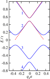
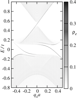
(a)    (b)   (c)

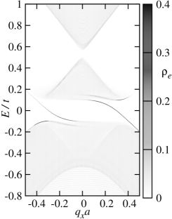
Figure 2: (Color online) (a) The eigenvalues of the BdG Hamiltonian in Eq. (1) (solid blue lines) and the effective gapped Dirac model in Eq. (21) (dashed red lines) vs. the deviation from the $K$ point, ${\bm{k}}_{K}=(0,4\pi/3\sqrt{3}a)$. (b) Energy spectrum obtained by exact diagonalization for a slab of 1200 layers in the $y$ direction and armchair edge. The eigenvalues are shaded according to the integrated electron-like weight in the first 40 laters of the slab. A dispersing edge resonance is clearly visible within the gap at the Dirac point near $E\approx 0.5t$. Two dispersing Andreev edge states are also present inside the superconducting gap near $E=0$. (c) Same as in panel (b), but with the inclusion of a Semenoff term $\delta_{s}=0.065t$, which renders the gap at the Dirac point topologically trivial. In all plots we set $\Delta=0.0866t$ and $\mu=-0.5t$.

IV Topological mass gap

Let us set the Semenoff term in Eq. (2) to zero first: $\delta_{s}=0$. In this case, there is no gap at the Dirac points $K$ and $K^{\prime}$ in the normal state. However, the energy spectrum of the BdG Hamiltonian in Eq. (1) shows an unexpected gap opening at the Dirac points near $E=\pm\mu=\pm 0.5t$ in Fig. 2(a), far away from the usual superconducting gap at the Fermi level $E=0$. Note that the momentum ${\bm{q}}={\bm{k}}-{\bm{k}}_{K}$ is measured relative to the $K$ point in Fig. 2.

To gain insight into the nature of this unexpected gap, we derive an effective Hamiltonian for the states near the Dirac points, perturbatively including the superconducting pairing in the limit $\Delta\ll|\mu|$. Our starting point is the formal expression for the electron-like component of the Green’s function,

$$\hbar G^{-1}({\bm{k}},\omega)$$

$$=\hbar\omega-H_{0}({\bm{k}})-\Delta({\bm{k}})\left[\hbar\omega+H_{0}^{T}(-{\bm{k}})\right]^{-1}\Delta^{\dagger}({\bm{k}})\,.$$ (20)

To find the energy spectrum in the vicinity of the Dirac points, we replace $\omega\to-\mu$ in the last term of Eq. (IV) and obtain an effective Hamiltonian

$$H_{\text{eff}}({\bm{k}})\approx H_{0}({\bm{k}})+\delta H\,.$$ (21)

Near the $K$ point, we can expand the first term to linear order in the relative momentum ${\bm{q}}={\bm{k}}-{\bm{k}}_{K}$

$$H_{0}({\bm{q}})=\left(\begin{array}[]{cc}-\mu&\frac{3}{2}ta(-q_{y}-iq_{x})\\ \frac{3}{2}ta(-q_{y}+iq_{x})&-\mu\end{array}\right)\,,$$ (22)

with the correction due to superconductivity

$$\delta H({\bm{k}}_{K})=-\frac{\Delta_{\pm}({\bm{k}}_{K})\Delta^{\dagger}_{\pm}({\bm{k}}_{K})}{2\mu}=-\frac{9|\Delta|^{2}}{4\mu}({s}_{0}\mp{s}_{z})\,.$$ (23)

Near the $K^{\prime}$ point, the expansion of the unperturbed Hamiltonian is identical except for the reversed sign in front of $q_{y}$, and the correction is

$$\delta H({\bm{k}}_{K^{\prime}})=-\frac{\Delta_{\pm}({\bm{k}}_{K^{\prime}})\Delta^{\dagger}_{\pm}({\bm{k}}_{K^{\prime}})}{2\mu}=-\frac{9|\Delta|^{2}}{4\mu}({s}_{0}\pm{s}_{z})\,.$$ (24)

Note that Eqs. (23) and (24) can be obtained from the last term in Eq. (IV) only in the vicinity of the Dirac points, where $H_{0}$ in Eq. (22) is proportional to the unit matrix in the limit of vanishing ${\bm{q}}$. Equation (21) can be interpreted as an effective normal-state Hamiltonian with the second-order perturbative correction due to superconducting pairing.

The perturbative correction given by Eqs. (23) and (24) is proportional to the matrix product $\Delta({\bm{k}})\Delta^{\dagger}({\bm{k}})$. Its time-reversal-even part, proportional to the unit matrix $s_{0}$, shifts the energy of the Dirac point. In contrast, the time-reversal-odd part (i.e., the TROB), proportional to $s_{z}$, opens a mass gap. This demonstrates the appearance of time-reversal symmetry breaking in the particle-hole channel due to the nonzero TROB. The gapped energy dispersion derived via this perturbative argument, shown by the dashed red curve in Fig. 2(a), is in excellent agreement with the dispersion of the full model near to the Dirac point.

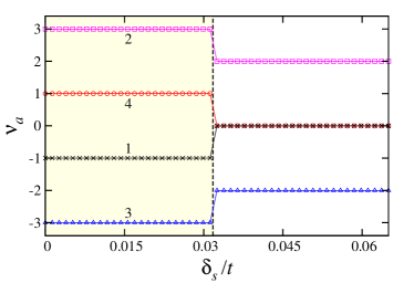
Figure 3: (Color online) Variation of the Chern numbers $\nu_{\alpha}$ of the four BdG bands labelled as in Fig. 2(a) vs. the Semenoff term $\delta_{s}$. The shaded region $\delta_{s}<\delta_{c}$ corresponds to the topologically nontrivial state. The lines are a guide for the eye. Other parameters are the same as in Fig. 2.

The mass gaps at the $K$ and $K^{\prime}$ points introduced by the superconductivity [Eqs. (23) and (24)] have opposite signs. This suggests a topologically nontrivial state, as in Haldane’s model of the quantum anomalous Hall state on the honeycomb lattice. Haldane1988 The topological nature of the mass gap is confirmed by calculation of the Chern numbers for the different bands and observation of chiral edge states within the energy gaps via the bulk-boundary correspondence. With the opening of the mass gap, the four eigenstates of the BdG Hamiltonian in Eq. (1) are everywhere nondegenerate, so a Chern number $\nu_{\alpha}$ can be defined for each band $\alpha=1,2,3,4$, as labeled in Fig. 2(a). As shown in Fig. 3, each band has a nonzero Chern number for $\delta_{s}=0$, i.e. in the absence of the Semenoff term. The sum of the Chern numbers of the occupied bands 3 and 4 below the chemical potential is $-2$, consistent with the chiral $d$-wave superconductivity. Correspondingly, the two topologically-protected chiral edge states within the superconducting gap are clearly visible near $E=0$ in the energy spectrum weighted by the integrated probability density of the electron-like wave function components near the surface, as shown in Fig. 2(b) for the armchair edge. The nonzero Chern numbers of the outer bands 1 and 4, which are separated by the mass gap from the inner bands 2 and 3, imply that the mass gap is topological. Thus, we would expect to find a single chiral edge state within each mass gap. However, due to the spectrum doubling in the superconducting state, the hole-like states generally overlap with the energy range of the mass gap and can hybridize with the edge state. Nevertheless, the edge state persists as a predominantly electron-like edge resonance inside the mass gap between bands 1 and 2 in Fig. 2(b).

A combination of a nonzero Semenoff term $\delta_{s}\neq 0$ in Eq. (2) and the superconducting corrections in Eqs. (23) and (24) produces different magnitudes of the mass gaps at the two Dirac points $K$ and $K^{\prime}$. At a critical value $\delta_{c}=\frac{1}{2}(\sqrt{9|\Delta|^{2}+\mu^{2}}-|\mu|)$, the gap at one of the Dirac points passes through zero and changes sign. Correspondingly, as shown in Fig. 3, there is an abrupt change in the Chern numbers of all BdG bands at this topological phase transition. For $|\delta_{s}|>\delta_{c}$, the Chern number of the outer bands 1 and 4 vanishes, although the sum of the Chern numbers of the occupied bands 3 and 4 remains $-2$. This is consistent with the mass gaps at $K$ and $K^{\prime}$ having the same sign, which is topologically trivial. Accordingly, we do not observe any edge resonance within the gap, as shown in Fig. 2(c).

Repeating the calculations for a zigzag edge, we also find evidence for Haldane states. However, they are mixed with the standard flat-band edge states that exist at the zigzag edges of a hexagonal lattice, making their interpretation more complicated.

V Loop currents

It was argued in the previous Section that the energy gaps observed at the Dirac points are similar to the energy gaps in Haldane’s model of the quantum anomalous Hall insulator. Haldane1988 They arise in Haldane’s model due to the presence of a time-reversal symmetry-breaking next-nearest-neighbor hopping term, resulting in loop currents around each lattice site shown by the arrows in Fig. 4. In second quantization, the time-reversal-odd part of this hopping term is proportional to the dimensionless operator $\chi_{lc}$, which is defined as

$$\chi_{lc} = i\sum_{{\bm{r}},\sigma}\left(a^{\dagger}_{{\bm{r}},\sigma}a_{{\bm{r}}+{\bm{c}}_{1},\sigma}+a^{\dagger}_{{\bm{r}}+{\bm{c}}_{1},\sigma}a_{{\bm{r}}+{\bm{c}}_{2},\sigma}+a^{\dagger}_{{\bm{r}}+{\bm{c}}_{2},\sigma}a_{{\bm{r}},\sigma}\right.$$ (25)

$$\left.+b^{\dagger}_{{\bm{r}},\sigma}b_{{\bm{r}}-{\bm{c}}_{1},\sigma}+b^{\dagger}_{{\bm{r}}-{\bm{c}}_{1},\sigma}b_{{\bm{r}}-{\bm{c}}_{2},\sigma}+b^{\dagger}_{{\bm{r}}-{\bm{c}}_{2},\sigma}b_{{\bm{r}},\sigma}-\mbox{H.c.}\right)$$

$$= \sum_{{\bm{k}}}4\sin(\tfrac{\sqrt{3}}{2}k_{y}a)\left[\cos(\tfrac{3}{2}k_{x}a)-\cos(\tfrac{\sqrt{3}}{2}k_{y}a)\right]$$

$$\times\Psi^{\dagger}_{\bm{k}}{\tau}_{0}\otimes{s}_{z}\Psi_{\bm{k}}\,.$$

Here ${\bm{c}}_{1}$ and ${\bm{c}}_{2}$ are the primitive lattice vectors (see Fig. 1), the operator $a_{{\bm{r}},\sigma}$ ($b_{{\bm{r}},\sigma}$) destroys a spin-$\sigma$ electron on the $A$ ($B$) site of the unit cell corresponding to the lattice vector ${\bm{r}}$, and ${\tau}_{0}$ is the unit matrix in Nambu space. The sign convention in Eq. (25) matches the convention for the link directions in Fig. 4.

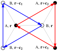
Figure 4: (Color online) Loop currents between the three nearest neighbors of the $A$ and $B$ sites in the unit cell at $\bm{r}$.

In Haldane’s model, the operator in Eq. (25) has a nonzero expectation value $\langle\chi_{lc}\rangle\neq 0$, resulting in the loop currents shown in Fig. 4. In our model, the operator $\chi_{lc}$ appears in the commutator (13) with the TROB given by Eq. (LABEL:eq:gapprod). The commutator of the pairing terms on the adjacent nearest-neighboring links generates electron transfer between the next-nearest neighboring sites with a complex amplitude carrying the phase difference of pairing potentials shown in Fig. 1. The analogy between our system and Haldane’s model suggests that $\chi_{lc}$ also has a non-zero expectation value in the chiral $d$-wave state, which is readily verified to be

$$\frac{\langle\chi_{lc}\rangle}{N} = -\frac{1}{N}\sum_{{\bm{k}}}\sin(\tfrac{\sqrt{3}}{2}k_{y}a)\left[\cos(\tfrac{3}{2}k_{x}a)-\cos(\tfrac{\sqrt{3}}{2}k_{y}a)\right]$$ (26)

$$\times\frac{1}{\beta}\sum_{\nu_{m}}\frac{8\mu\,\Xi_{\pm}({\bm{k}})}{(\hbar^{2}\nu_{m}^{2}+E_{{\bm{k}},1}^{2})(\hbar^{2}\nu_{m}^{2}+E_{{\bm{k}},2}^{2})}\,.$$

Here $E_{{\bm{k}},\alpha=1,2}>0$ are the quasiparticle dispersions corresponding to the upper two bands shown in Fig. 2(a) (explicit expressions are given in LABEL:BlaSchPRB2014), $\beta=1/k_{B}T$ is the inverse temperature, $\nu_{m}$ are the fermionic Matsubara frequencies, and $N$ is the number of unit cells. The presence in Eq. (26) of the sublattice polarization $\Xi_{\pm}({\bm{k}})$ from Eq. (16) (equivalent to the TROB) is essential for obtaining a nonzero expectation value of $\chi_{\text{lc}}$. Since $\Xi_{\pm}({\bm{k}})$ has the same momentum dependence as the term in front of the fraction in Eq. (26), the summand has the same sign everywhere in the Brillouin zone, and thus the expectation value $\langle\chi_{lc}\rangle$ is nonzero. The essential importance of the TROB in ensuring $\langle\chi_{lc}\rangle\neq 0$ is consistent with the role of the TROB in generating the energy gaps at the Dirac points. As such, the inclusion of the Semenoff term does not alter the conditions for a nonzero expectation value of $\langle\chi_{lc}\rangle$, but Eq. (26) is replaced by a more complicated expression given in Appendix C. We note that $\langle\chi_{lc}\rangle\neq 0$ was calculated in LABEL:Faye2015 for the closely-related nearest-neighbor chiral $p$-wave state introduced in Appendix A. In contrast, $\langle\chi_{lc}\rangle$ is zero for the intra-sublattice chiral $d$-wave state described by Eq. (III), where the TROB vanishes.

However, unlike in Haldane’s model, a nonzero expectation value of $\chi_{lc}$ in our system only implies the presence of loop current correlations. Since the normal-state Hamiltonian (2) does not contain next-nearest-neighbor hopping, there are no current operators between next-nearest sites in our model. We can remedy this by introducing a next-nearest-neighbor hopping term with a small real amplitude $t^{\prime}$:

$$H_{t^{\prime}}=t^{\prime}\sum_{\langle\langle m,n\rangle\rangle,\sigma}(a_{{\bm{r}}_{m},\sigma}^{\dagger}a_{{\bm{r}}_{n},\sigma}+b_{{\bm{r}}_{m},\sigma}^{\dagger}b_{{\bm{r}}_{n},\sigma}).$$ (27)

The corresponding current operators between the next-nearest-neighbor sites $m$ and $n$ belonging to the sublattice $c=A,B$ are hence obtained from Eq. (27) as

$$I^{c}_{mn}=\frac{iet^{\prime}}{\hbar}\left[\psi^{\dagger}_{c,\sigma}({\bm{r}}_{m})\psi_{c,\sigma}({\bm{r}}_{n})-\psi^{\dagger}_{c,\sigma}({\bm{r}}_{n})\psi_{c,\sigma}({\bm{r}}_{m})\right],$$ (28)

where $\psi_{c,\sigma}({\bm{r}})$ is the annihilation operator for spin-$\sigma$ electrons on sublattice $c$ of unit cell ${\bf r}$. Adding the current operators in Eq. (28) with the signs corresponding to Fig. 4, we introduce the total current operator $I_{\rm tot}$ as

$$I_{\rm tot}=\frac{et^{\prime}}{\hbar}\chi_{lc}\,.$$ (29)

Then the expectation value $I$ of the microscopic current on one link is obtained as

$$I=\frac{\langle I_{\rm tot}\rangle}{6N}=\frac{et^{\prime}}{6\hbar}\frac{\langle\chi_{lc}\rangle}{N},$$ (30)

where we divide by $6$ because there are six currents of equal magnitude in a unit cell. The current $I$ is very small, because it is proportional to the small hopping amplitude $t^{\prime}$ and $\langle\chi_{lc}\rangle/N\sim\mu\Delta^{2}/t^{3}\ll 1$ from Eq. (26).

Another physical consequence of $\langle\chi_{lc}\rangle\neq 0$ is the existence of a nonzero anomalous Hall conductivity in the absence of an external magnetic field, which is calculated in the next Section. Unlike the current $I$ in Eq. (30), the Hall conductivity does not require $t^{\prime}\neq 0$, so we set $t^{\prime}=0$ in the rest of the paper to simplify calculations.

VI Hall conductivity

The existence of loop-current correlations in Eq. (26) for the chiral $d$-wave state naturally suggests the presence of an intrinsic Hall conductivity. Indeed, the nontrivial sublattice structure of the BdG Hamiltonian (1) is consistent with the conditions outlined in LABEL:Taylor2012 for the existence of an intrinsic Hall effect.

As shown by the Feynman diagrams in Fig. 5, the Hall conductivity can be obtained as the difference

$$\sigma_{H}(\omega)=\frac{i}{2\hbar\omega}\lim_{i\omega_{n}\to\omega+i0^{+}}\left[\pi_{xy}(i\omega_{n})-\pi_{yx}(i\omega_{n})\right]$$ (31)

of the current-current correlation functions

$$\pi_{ab}(i\omega_{n})=-\frac{1}{S}\int^{\hbar\beta}_{0}d\tau e^{i\omega_{n}\tau}\left\langle T_{\tau}J_{a}(\tau)J_{b}(0)\right\rangle,$$ (32)

where $\omega_{n}$ is a bosonic Matsubara frequency and $S$ is the total area of the crystal. Here $J_{a}$ is the $a$-component of the current operator

$${\bm{J}}=e\sum_{\bm{k}}\Psi^{\dagger}_{\bm{k}}{\bm{V}}_{\bm{k}}\Psi_{\bm{k}},$$ (33)

where ${\bm{V}}_{\bm{k}}$ is the velocity vertex in Nambu notation

$${\bm{V}}_{\bm{k}}={\tau}_{0}\otimes\left(\begin{array}[]{cc}0&{\bm{v}}_{\bm{k}}\\ {\bm{v}}_{\bm{k}}^{\ast}&0\end{array}\right),$$ (34)

and the velocity components are obtained from Eq. (3).

$${\bm{v}}_{\bm{k}}=\frac{1}{\hbar}\frac{\partial}{\partial\bm{k}}(\epsilon^{x}_{\bm{k}}-i\epsilon^{y}_{\bm{k}})=-\frac{it}{\hbar}\sum_{j}\bm{R}_{j}e^{i\bm{k}\cdot\bm{R}_{j}}$$ (35)

A straightforward evaluation of the Feynman diagrams in Fig. 5 (for the vanishing Semenoff term $\delta_{s}=0$) yields the Hall conductivity

$$\sigma_{H}(\omega)=\lim_{i\omega_{n}\to\omega+i0^{+}}\frac{1}{\beta}\sum_{\nu_{m}}\int\frac{d^{2}k}{(2\pi)^{2}}\frac{e^{2}\hbar^{3}\mu\,i[{\bm{v}}_{\bm{k}}^{*}\wedge{\bm{v}}_{\bm{k}}]\,\Xi_{\pm}({\bm{k}})\,(i\omega_{n}+2i\nu_{m})^{2}}{(\hbar^{2}\nu_{m}^{2}+E_{{\bm{k}},1}^{2})(\hbar^{2}\nu_{m}^{2}+E_{{\bm{k}},2}^{2})(\hbar^{2}[\omega_{n}+\nu_{m}]^{2}+E_{{\bm{k}},1}^{2})(\hbar^{2}[\omega_{n}+\nu_{m}]^{2}+E_{{\bm{k}},2}^{2})}.$$ (36)

The sign of $\sigma_{H}(\omega)$ correlates with the sign of the chemical potential $\mu$, and the Hall conductivity vanishes at $\mu=0$ (at the Dirac point) due to particle-hole symmetry. The real and imaginary parts of the Hall conductivity calculated from Eq. (36) are shown in Fig. 6. This expression is consistent with Eq. (24) of LABEL:KerrUPt3_theory for the Hall conductivity in UPt₃ in the limiting case where spin-orbit coupling and intrasublattice hopping terms are neglected. As the point groups of UPt₃ and the honeycomb lattice are both $D_{6h}$, such terms are also allowed in our model, but we neglect them for simplicity.

Equation (36) shows some similarity to a general formulaTewari2008 for the intrinsic ac Hall conductivity in terms of the Berry curvature for a nonsuperconducting two-band system, which includes Haldane’s model. However, that formula is not directly applicable to our superconducting case, because the effective two-band model derived in Sec. IV is only suitable near to the Dirac points.

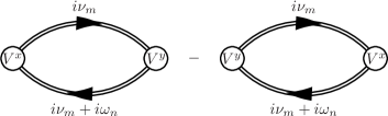
Figure 5: Feynman diagrams for the intrinsic Hall conductivity. The double lines are the matrix superconducting Green’s functions in Nambu notation. The vertices ${V}^{x}$ and ${V}^{y}$ are the $x$- and $y$-components of the velocity operator in Eq. (34). The Matsubara frequencies $i\omega_{n}$ and $i\nu_{m}$ are the external bosonic and internal fermionic frequencies, respectively.

Figure 6: (Color online) Real (solid red line) and imaginary (dashed blue line) parts of the Hall conductivity calculated using Eq. (36). The high-frequency approximation from Eq. (40) (black dotted line) agrees very well with the exact result for $\hbar\omega\gtrsim 4t$. The inset compares the approximate and exact results in more detail. We use the same parameters as in Fig. 2(a) and set the temperature $k_{B}T=0.05t$.

From the numerator of Eq. (36), it is clear that the anomalous Hall conductivity $\sigma_{H}(\omega)$ is nonzero only when the sublattice polarization $\Xi_{\pm}(\bm{k})$ in Eq. (16) has common irreducible representations with the product of velocities $[{\bm{v}}_{\bm{k}}\wedge{\bm{v}}_{\bm{k}}^{*}]$. Indeed, we find from Eq. (35) that

$$[{\bm{v}}_{\bm{k}}\wedge{\bm{v}}_{\bm{k}}^{*}]=\frac{2it^{2}a^{2}}{\hbar^{2}}\sum_{j<j^{\prime}}\sin(\varphi_{j^{\prime}}-\varphi_{j})\,\sin[\bm{k}\cdot(\bm{R}_{j}-\bm{R}_{j^{\prime}})],$$ (37)

where $\varphi_{j}$ are the geometric angles between the vectors $\bm{R}_{j}$ and the $x$ axis, which, in our model, are the same as the phases $\phi_{j}$ in Eq. (4). Thus, Eq. (37) has the same momentum dependence as the TROB in Eq. (LABEL:eq:gapprod) and $\Xi_{\pm}(\bm{k})$ in Eq. (16).

The full result Eq. (36) is rather complicated, but it simplifies in the high-frequency limit $\hbar\omega\gg t$. This regime is experimentally relevant, as the polar Kerr effect measurements detailed in LABEL:KapNJP2009 are performed at infrared frequency $\hbar\omega=0.8$eV which is typically large compared to the hopping integrals in a strongly-correlated material. As shown in LABEL:Shastry1993, the Hall conductivity in this limit is given by

$$\sigma_{H}(\omega)\approx\frac{i}{S\hbar\omega^{2}}\langle\left[J_{x},J_{y}\right]\rangle\,.$$ (38)

Taking into account Eq. (37), we find that the commutator of the $x$- and $y$-components of the current operator appearing in this expression is directly proportional to the loop-current operator in Eq. (25)

$$\left[J_{x},J_{y}\right]=e^{2}\sum_{\bm{k}}{[{\bm{v}}_{\bm{k}}\wedge{\bm{v}}_{\bm{k}}^{*}]}\,\Psi^{\dagger}_{\bm{k}}{\tau}_{0}\otimes{s}_{z}\Psi_{\bm{k}}=\frac{\sqrt{3}ie^{2}t^{2}a^{2}}{2\hbar^{2}}\chi_{lc}\,.$$ (39)

We hence find that the high-frequency Hall conductivity is proportional to the expectation value of the loop-current operator:

$$\sigma_{H}(\omega)\approx-\frac{\sqrt{3}e^{2}t^{2}a^{2}}{2S\hbar^{3}\omega^{2}}\langle\chi_{lc}\rangle$$ (40)

$$=\frac{2e^{2}}{\hbar\omega^{2}}\frac{1}{\beta}\sum_{\nu_{m}}\int\frac{d^{2}k}{(2\pi)^{2}}\frac{\mu i[{\bm{v}}_{\bm{k}}^{*}\wedge{\bm{v}}_{\bm{k}}]\,\Xi_{\pm}({\bm{k}})}{(\hbar^{2}\nu_{m}^{2}+E_{{\bm{k}},1}^{2})(\hbar^{2}\nu_{m}^{2}+E_{{\bm{k}},2}^{2})}\,.$$

Equations (38)–(40) establish a direct connection between the Hall conductivity and the loop currents discussed in Sec. IV. As shown in Fig. 6, the agreement between Eqs. (36) and (40) is very good for $\hbar\omega\gtrsim 4t$. An alternative derivation is presented in Appendix D in the limit of small $\Delta$, where the Green’s functions appearing in Fig. 5 can be expanded to the second order in the pairing potential. This approach yields Eq. (D) similar to Eq. (40), but with the BdG energies $E_{\bm{k}}$ replaced by the normal-state energies $\epsilon_{\bm{k}}$.

The high-frequency Hall conductivity in Eq. (40) is real, but the polar Kerr effect is primarily sensitive to the imaginary part of the Hall conductivity when the refraction index is predominantly real. KapNJP2009 Although it is not possible to directly associate the imaginary part of the Hall conductivity at a given frequency to the loop currents in the superconductor, an indirect connection is provided by the sum rule Lange1999

$$\int\limits^{\infty}_{-\infty}\omega\text{Im}\{\sigma_{H}(\omega)\}d\omega=-\frac{i\pi}{\hbar S}\langle\left[J_{x},J_{y}\right]\rangle=\frac{\pi\sqrt{3}e^{2}t^{2}a^{2}}{2S\hbar^{3}}\langle\chi_{lc}\rangle\,.$$

Again, the right-hand side of this equation is proportional to the expectation value of the loop-current operator, and we hence conclude that the existence of the loop-current correlations results in a nonzero imaginary Hall conductivity.

It should be noted that, in contrast to nonsuperconductors, the dc Hall conductivity in superconductors is not directly related to the Chern number, as discussed in Appendices A and B of LABEL:Lutchyn2009. Thus, the topological phase diagram shown in Fig. 3 in terms of the Semenoff term $\delta_{s}$ is not particularly relevant for the calculation of the Hall conductivity. A generalization of Eq. (36) to a nonzero Semenoff term in Appendix C shows that the ac Hall conductivity $\sigma_{H}(\omega)$ is nonzero for any value of $\delta_{s}$. Moreover, in the high-frequency limit, Eqs. (38) and (39) are still valid for $\delta_{s}\neq 0$, so the Hall conductivity remains proportional to the expectation value of the loop-current operator, which is mainly sensitive to the pairing potential and only weakly dependent upon the Semenoff term.

VII Phenomenological treatment

In Eq. (26) we obtained a nonzero expectation value of the loop-current operator from a microscopic theory of the chiral $d$-wave state at the level of the single-particle Green’s functions. The appropriate interactions would, however, lead to true long-range loop-current order. The interplay of this order with the superconductivity could then be understood within the framework of a phenomenological Landau expansion of the free energy density

$$f-f_{0} = \alpha(|\eta_{1}|^{2}+|\eta_{2}|^{2})+\beta_{1}(|\eta_{1}|^{2}+|\eta_{2}|^{2})^{2}$$ (41)

$$+\beta_{2}(\eta_{1}^{\ast}\eta_{2}-\eta_{1}\eta_{2}^{\ast})^{2}$$

$$+i\gamma\delta_{lc}(\eta_{1}^{\ast}\eta_{2}-\eta_{1}\eta_{2}^{\ast})+\kappa\delta_{lc}^{2}\,,$$

where $f_{0}$ is the normal-state free energy density. The first two lines describe the superconductivity, where $\eta_{1}$ and $\eta_{2}$ are the order parameters corresponding to the two states in the $E_{2g}$ irreducible representation. The term with $\beta_{2}>0$ stabilizes the time-reversal symmetry-breaking configuration $(\eta_{1},\eta_{2})\propto(1,\pm i)$ studied in this paper. The coupling to the loop-current order parameter $\delta_{lc}\propto\langle\chi_{lc}\rangle$ is given by $\gamma$, and $\kappa>0$ implies that this order is subdominant. Minimization of $f$ with respect to $\delta_{lc}$ shows that the loop-current order becomes induced in the time-reversal-breaking superconducting state.

As already mentioned in Sec. III, a more intriguing possibility could be that the loop-current order preempts the superconductivity. We speculate that fluctuating superconducting order may cause the discrete $\mathbb{Z}_{2}$ time-reversal symmetry to be broken with $\delta_{lc}\neq 0$ at a higher temperature than the continuous $U(1)$ gauge symmetry, which is rigorously permitted only at zero temperature in two dimensions. Similar scenarios were discussed for multiband superconductors in LABEL:Babaev and for pair-density wave order in the underdoped cuprates in LABEL:cuprate.

VIII Relevance to superconductivity in twisted bilayer graphene

It has been proposed theoretically Wu2018 ; Xu2018 ; Fidrysiak2018 ; Guo2018 ; Su2018 ; Liu2018 that the superconducting state observed in twisted bilayer graphene Cao2018 (TBLG) realizes chiral $d$-wave pairing. Given that our analysis concerns hypothetical superconductivity in monolayer graphene, it is worthwhile to survey theories of TBLG briefly and explore possible links to our work. Although most proposals include more electronic degrees of freedom than our model, in many cases they show a qualitative resemblance, implying that the physics discussed in our paper may be applicable.

Some of the earliest proposals, such as Refs. Xu2018, ; Fidrysiak2018, , assume $SU(4)$ symmetry of a single-particle Hamiltonian, for which the physics we discuss does not apply. However, $SU(4)$ symmetry-breaking terms may change this conclusion and are currently under consideration.

Phenomenological models with orbital or sublattice degrees of freedom have been considered in Refs. Dodaro2018, and Guo2018, , respectively. Due to the presence of these additional electronic degrees of freedom, the pairing potential may have a nonzero TROB, thus resulting in similar physics to that discussed here. The model of Ref. Guo2018, , based upon a three-site sublattice to simulate the AA and AB regions of the Moiré pattern of TBLG, resembles our model most closely and, indeed, reduces to it in the limit $t^{\prime}=\Delta^{\prime}_{j}=0$, where the triangular lattice of the AA regions is neglected.

Several papers Quan2018 ; Koshino2018 ; Kang2018 ; Po2018 proposed a low-energy description of the normal-state electronic structure based on an emergent honeycomb lattice with two additional electronic orbital degrees of freedom at each lattice site. Reference Liu2018, considers such a model with $p_{x}$ and $p_{y}$ orbitals on a honeycomb lattice with local electronic interactions and finds that a $d$-wave chiral pairing state emerges. The paper argues that the mechanism is similar to that for chiral $d$-wave pairing in single-layer graphene at quarter doping, for which our model applies.

Adopting an alternative approach, Refs. Su2018, and Wu2018, numerically analyze how a nearest-neighbor chiral $d$-wave state in each of the two graphene layers is modified by the Moiré structure in TBLG. Interestingly, these papers find intra-unit-cell supercurrent loops. Since the intralayer pairing state is identical to ours, we suggest that these currents may be related to the loop current correlations found in our work.

Although a theoretical description of the superconducting state in TBLG remains unsettled, the presence of multiple electronic degrees of freedom indicates that a chiral $d$-wave state is likely to have a nonvanishing TROB. Consequently, much of the physics discussed in our paper may be applicable. An experimental measurement of the polar Kerr effect in TBLG would be particularly useful to verify whether the superconducting pairing breaks time-reversal symmetry.

IX Conclusions

In this paper we have examined the appearance of the polar Kerr effect in a minimal model of time-reversal symmetry-breaking chiral $d$-wave superconductivity on the honeycomb lattice. We have demonstrated that the existence of a gauge-invariant time-reversal-odd bilinear (TROB) constructed from the pairing potential is an essential requirement for the polar Kerr effect. In the context of the honeycomb lattice, the TROB reflects the sublattice polarization of the pairing. The key physical manifestation of the TROB is the appearance of an emergent nonsuperconducting order in conjunction with the superconductivity, which we identify as loop currents similar to those in Haldane’s model of a quantum anomalous Hall insulator. Haldane1988 This is directly evidenced in the energy spectrum, where we observe the opening of a topological gap with opposite signs at the Dirac points $K$ and $K^{\prime}$. The Kubo formula calculation of the intrinsic ac Hall conductivity in the absence of an external magnetic field shows that it is directly proportional to the expectation value of the loop current operator. Thus we establish an explicit relation connecting the emergent loop-current correlations and both the real and imaginary parts of the Hall conductivity.

The model considered here is another example of a time-reversal symmetry-breaking superconducting state with an intrinsic Hall conductivity, and generalizes these analyses to an even-parity pairing state. The first example is Sr₂RuO₄, where different pairing in the Ru $d_{xz}$ and $d_{yz}$ orbitals implies a polarization in the $d_{xz}$-$d_{yz}$ orbital space. Wysokinski2012 ; Taylor2012 ; GradhandSr2RuO4 ; RobbinsSr2RuO4 ; KomendovaPRL2017 More recently, a theoretical treatment of the Kerr effect in UPt₃ has identified the time-reversal-odd sublattice dependence of the pairing potential permitted by the nonsymmorphic symmetry as an essential ingredient. KerrUPt3_theory ; Yanase2016 The similarity of these models to the simpler case considered in our paper suggests the intriguing possibility that the Hall conductivities in these systems can be also understood in terms of loop-current correlations induced by a TROB. Although we have considered only two internal degrees of freedom here, loop currents can also arise in materials with more complicated unit cells, Ghosh2018 including twisted bilayer graphene. The observation of the polar Kerr effect in many unconventional superconductors therefore suggests that pairing states supporting nonzero TROBs may be realized in a broad range of materials.

Appendix A Chiral $p$-wave state

Other chiral pairing states on the honeycomb lattice also display a polarization in their sublattice degrees of freedom due to a non-zero TROB. For example, chiral $p$-wave triplet superconductivity with nearest-neighbor pairing has been considered by several authors. Xu2016 ; Faye2015 ; QiFuSunGu2017 ; Ying2017 Here we examine the case where the vector $\bm{d}$ of the triplet pairing is oriented along the $z$ axis, which is also the spin quantization axis. In this representation, the triplet pairing takes place between the opposite spins and is described by the BdG Hamiltonian in Eq. (1) with the pairing potential

$${\Delta}_{\pm}^{p}({\bm{k}})=\Delta\sum\limits_{j=1}^{3}e^{\pm i\phi_{j}}\left(\begin{array}[]{cc}0&e^{i{\bm{k}}\cdot{\bm{R}}_{j}}\\ -e^{-i{\bm{k}}\cdot{\bm{R}}_{j}}&0\end{array}\right)\,.$$ (42)

Note that one of the off-diagonal terms has opposite sign compared with Eq. (4) for the pairing potential of the chiral $d$-wave state, but the phases along each bond $\phi_{j}=(j-1)2\pi/3$ are the same. As shown in Fig. 7, the phase of the pairing on each bond winds by $2\pi$ as one moves around a hexagonal plaquette, in contrast to the chiral $d$-wave state where the phase winds by $4\pi$.

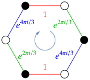
(a)(b)

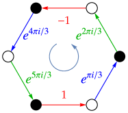
Figure 7: (Color online) Phases of the nearest-neighbor pairing potentials on the bonds of a hexagonal plaquette for the (a) chiral $d$-wave state and (b) the chiral $p$-wave state. In the former the phase winds by $4\pi$ around the plaquette, whereas in the latter in winds by $2\pi$, and the direction of winding is indicated by the curved arrow. In the spin-triplet $p$-wave state, the straight arrow points to the location of the spin-$\downarrow$ electron in the Cooper pair for the given phase. Placing the spin-$\downarrow$ electron at the other end of the arrow gives an overall sign change of the pairing potential.

The pairing potential in Eq. (42) can be decomposed into basis states of the irreducible representation $E_{1u}$

$${\Delta}^{p}_{\pm}({\bm{k}})={\Delta}^{p}_{x}({\bm{k}})\pm i{\Delta}^{p}_{y}({\bm{k}}),$$ (43)

where

$${\Delta}^{p}_{x}({\bm{k}}) = i\Delta\left\{\left[\cos(k_{x}a)-\cos(\tfrac{1}{2}k_{x}a)\cos(\tfrac{\sqrt{3}}{2}k_{y}a)\right]{s}_{y}\right.$$

$$\left.+\left[\sin(k_{x}a)+\sin(\tfrac{1}{2}k_{x}a)\cos(\tfrac{\sqrt{3}}{2}k_{y}a)\right]{s}_{x}\right\},$$

$${\Delta}^{p}_{y}({\bm{k}}) = i\sqrt{3}\Delta\left\{\sin(\tfrac{1}{2}k_{x}a)\sin(\tfrac{\sqrt{3}}{2}k_{y}a){s}_{y}\right.$$

$$\left.+\cos(\tfrac{1}{2}k_{x}a)\sin(\tfrac{\sqrt{3}}{2}k_{y}a){s}_{x}\right\}.$$

Projected onto the states at the Fermi surface, the basis functions ${\Delta}^{p}_{x}({\bm{k}})$ and ${\Delta}^{p}_{y}({\bm{k}})$ appear as $p_{x}$-wave and $p_{y}$-wave triplet states, respectively. Like the basis functions for $E_{2g}$ discussed in Sec, II, these states contain the matrices ${s}_{x}$ and ${s}_{y}$, but here with odd- and even-parity coefficients, respectively. This ensures that the pairing potentials are odd under inversion, i.e. ${\cal I}^{\dagger}\Delta^{p}_{x}({\bm{k}}){\cal I}=-\Delta^{p}_{x}(-{\bm{k}})$.

The $E_{1u}$ basis functions can be obtained from the basis functions for $E_{2g}$ by multiplying them with ${s}_{z}$. This follows from the direct product rules for the point group $D_{6h}$, since $s_{z}$ belongs to the irreducible representation $B_{1u}$ and $E_{1u}=B_{1u}\times E_{2g}$. Thus, the TROB of the chiral $p$-wave state is the same as for the chiral $d$-wave case in Eq. (LABEL:eq:gapprod):

TROB

$$=\mp 4\sqrt{3}|\Delta|^{2}\sin(\tfrac{\sqrt{3}}{2}k_{y}a)\left[\cos(\tfrac{3}{2}k_{x}a)-\cos(\tfrac{\sqrt{3}}{2}k_{y}a)\right]{s}_{z}\,.$$

The physics arising from the existence of the TROB in the chiral $p$-wave state is thus essentially the same as for the chiral $d$-wave state discussed in the main part of the paper.

We finally note that, in the presence of a Semenoff term, the reduced symmetry of the lattice due to lack of inversion implies that both the $p$-wave and $d$-wave pairing potentials are basis states of the same irreducible representation $E^{\prime}$ of the point group $D_{3h}$. As such, a chiral state can generally involve a mixture of the two. BlackSchaeffer2015 ; QiFuSunGu2017

Appendix B Time-reversal odd bilinear in more general models

Here we show that Eq. (12) for the TROB applies quite generally, including Hamiltonians with spin-orbit coupling and more electronic degrees of freedom, and without inversion symmetry.

The pairing term in Eq. (1) couples opposite spins, but a more general BdG Hamiltonian can be written in terms of a $2m$-component operator $c_{\bm{k}}$ encoding $m$ orbital or sublattice degrees of freedom (assumed to be time-reversal invariant) and both spin orientations:

$$H=\frac{1}{2}\sum_{\bm{k}}\Psi^{\dagger}_{\bm{k}}{\cal H}_{\bm{k}}\Psi_{\bm{k}}\,.$$ (44)

Here $\Psi_{\bm{k}}=(c_{\bm{k}},c^{\dagger}_{-{\bm{k}}})^{T}$ is a Nambu spinor, and $T$ denotes transposition. We use $\hat{\Delta}(\bm{k})$ with a “hat” to denote pairing potential in this basis:

$${\cal H}_{\bm{k}}=\left(\begin{array}[]{cc}H_{0}(\bm{k})&\hat{\Delta}(\bm{k})\\ \hat{\Delta}^{\dagger}(\bm{k})&-H_{0}^{T}(-\bm{k})\end{array}\right).$$ (45)

The pairing potential obeys $\hat{\Delta}^{T}(\bm{k})=-\hat{\Delta}(-\bm{k})$ due to the fermion exchange symmetry. SPOT

The time-reversal operation is implemented as $\Theta={\cal K}U$, where $\cal K$ is complex conjugation, and the unitary part Agterberg2017 is

$$U=i\sigma_{y}\otimes s_{0}=\left(\begin{array}[]{rr}0&1\\ -1&0\end{array}\right)\otimes s_{0}\,.$$ (46)

Here $\sigma_{y}$ is the spin Pauli matrix, and $s_{0}$ is an $m$-dimensional identity matrix operating on the $m$ orbital or sublattice electronic degrees of freedom. The matrix $U$ is real and satisfies $U^{2}=-1$ and $U^{\dagger}=U^{T}=U^{-1}=-U$. Because it is real, the creation and annihilation operators transform upon time reversal in the same way, as discussed in Sec. III:

$$c_{\bm{k}} \;\to\; \Theta c_{\bm{k}}\Theta^{-1}=Uc_{-\bm{k}}$$

$$c^{\dagger}_{\bm{k}} \;\to\; \Theta c^{\dagger}_{\bm{k}}\Theta^{-1}=Uc^{\dagger}_{-\bm{k}}$$

$$\Psi_{\bm{k}} \;\to\; \Theta\Psi_{\bm{k}}\Theta^{-1}=[\tau_{0}\otimes U]\,\Psi_{-\bm{k}}\,,$$

where $\tau_{0}$ is a $2\times 2$ identity matrix in the Nambu space. The matrix elements in Eq. (45) become complex-conjugated upon time reversal: ${\cal H}_{\bm{k}}\to\Theta{\cal H}_{\bm{k}}\Theta^{-1}={\cal H}_{\bm{k}}^{*}$. Combining these transformations, we obtain the time reversal of the BdG Hamiltonian (44)

$$H \;\to\; \frac{1}{2}\sum_{\bm{k}}\Theta\Psi^{\dagger}_{\bm{k}}\Theta^{-1}\Theta{\cal H}_{\bm{k}}\Theta^{-1}\Theta\Psi_{\bm{k}}\Theta^{-1}$$

$$= \frac{1}{2}\sum_{\bm{k}}\Psi_{-\bm{k}}^{\dagger}\,[\tau_{0}\otimes U^{T}]\,{\cal H}_{\bm{k}}^{*}\,[\tau_{0}\otimes U]\,\Psi_{-\bm{k}}\,.$$

Changing $\bm{k}\to-\bm{k}$ in the sum, we arrive to a BdG Hamiltonian of the same form as in Eq. (44) but with the transformed matrix elements in Eq. (45)

$${\cal H}_{\bm{k}}\;\to\;[\tau_{0}\otimes U^{T}]\,{\cal H}^{*}_{-\bm{k}}\,[\tau_{0}\otimes U].$$ (47)

The time-reversal rule in Eq. (47) is similar to that for a non-superconducting Hamiltonian, Bernevig because $U$ is real.

According to Eq. (47), the pairing potential transforms as

$$\hat{\Delta}(\bm{k})\;\to\;U^{T}\hat{\Delta}^{*}(-\bm{k})U=-U^{T}\hat{\Delta}^{\dagger}(\bm{k})U,$$ (48)

where we used the fermion exchange relation. It is convenient to define $\Delta({\bm{k}})$ without the “hat” as

$$\Delta({\bm{k}})=\hat{\Delta}({\bm{k}})U,$$ (49)

which corresponds more closely to the pairing potential introduced in Sec. II. Combining Eq. (48) with Eq. (49) and using $U^{2}=-1$, we reproduce Eq. (11)

$$\Delta(\bm{k})\to\Delta^{\dagger}(\bm{k}).$$ (50)

Finally, we obtain the TROB as the difference between $\hat{\Delta}({\bm{k}})\hat{\Delta}^{\dagger}({\bm{k}})$ and its time-reversed counterpart:

TROB $$= \hat{\Delta}({\bm{k}})\hat{\Delta}^{\dagger}({\bm{k}})-\Theta\hat{\Delta}({\bm{k}})\Theta^{-1}\Theta\hat{\Delta}^{\dagger}({\bm{k}})\Theta^{-1}$$ (51)

$$= \hat{\Delta}({\bm{k}})\hat{\Delta}^{\dagger}({\bm{k}})-U^{T}\hat{\Delta}^{\dagger}({\bm{k}})\hat{\Delta}({\bm{k}})U$$

$$= \Delta(\bm{k})\Delta^{\dagger}(\bm{k})-\Delta^{\dagger}(\bm{k})\Delta(\bm{k}),$$

where we used Eqs. (48) and (49). Equation (51) reproduces Eq. (12) for the TROB, which is the result we wanted to show in general form.

As discussed in Sec. III, the superconducting fitness restricts opportunities for a nonzero TROB. The general condition for superconducting fitness Ramires2016 ; Ramires2018 is

$$H_{0}(\bm{k})\hat{\Delta}(\bm{k})=\hat{\Delta}(\bm{k})H_{0}^{*}(-\bm{k}).$$ (52)

If the normal-state Hamiltonian $H_{0}(\bm{k})$ is invariant under time reversal in Eq. (47), then, using Eq. (49), Eq. (52) reduces to the commutator in Eq. (17)

$$[H_{0}({\bm{k}}),\Delta({\bm{k}})]=0.$$ (53)

Below we illustrate these general relations by simple examples. For a single-band superconductor, where the only internal degree of freedom is spin, the pairing potential can be written in terms of the spin Pauli matrices

$$\Delta({\bm{k}})=\Delta^{(s)}_{\bm{k}}+\Delta^{(t)}_{\bm{k}}({\bm{d}}_{\bm{k}}\cdot\bm{\sigma}).$$ (54)

Here $\Delta^{(s)}_{\bm{k}}$ and $\Delta^{(t)}_{\bm{k}}$ represent singlet and triplet pairing, and $\bm{d}_{\bm{k}}$ is a unit vector. Evaluation of Eq. (51) for this pairing potential gives

$$\mbox{TROB}=2i\,|\Delta^{(t)}_{\bm{k}}|^{2}\,(\bm{d}_{\bm{k}}\times\bm{d}^{*}_{\bm{k}})\cdot\bm{\sigma}.$$ (55)

Clearly, $\mbox{TROB}\neq 0$ only when the vector $\bm{d}^{*}_{\bm{k}}$ is not parallel to $\bm{d}_{\bm{k}}$. The pairing with $\bm{d}_{\bm{k}}\times\bm{d}^{*}_{\bm{k}}\neq 0$ is known in the literature SigUeda1991 as nonunitary pairing, because the product $\Delta(\bm{k})\Delta^{\dagger}(\bm{k})$ is not proportional to the unit matrix. Obviously, TROB in Eq. (51) vanishes for a unitary pairing, so nonunitarity is a necessary, but generally not sufficient condition for $\mbox{TROB}\neq 0$.

A similar construction can be obtained for spin-singlet pairing in a two-band model, where the pairing potential is expanded in the Pauli matrices $s_{\lambda}$ for sublattice space:

$$\Delta({\bm{k}})=\Delta^{(0)}_{\bm{k}}s_{0}+\bm{\Delta}_{\bm{k}}\cdot{\bm{s}}.$$ (56)

The honeycomb lattice model described in Sec. II is a special case where $\Delta^{(0)}=0$ and the vector $\bm{\Delta}_{\bm{k}}$ has only two components. An evaluation of Eq. (51) for Eq. (56) gives a formula similar to Eq. (55)

$$\mbox{TROB}=[\Delta({\bm{k}}),\Delta^{\dagger}({\bm{k}})]=2i(\bm{\Delta}_{\bm{k}}\times\bm{\Delta}^{*}_{\bm{k}})\cdot{\bm{s}}.$$ (57)

For $\mbox{TROB}\neq 0$, the pairing vector $\bm{\Delta}_{\bm{k}}$ must be not parallel to its complex conjugate.

To evaluate the fitness condition for this model, we take the normal-state Hamiltonian to be spin-independent and write it as

$$H_{0}({\bm{k}})=h^{(0)}_{\bm{k}}s_{0}+{\bm{h}}_{\bm{k}}\cdot{\bm{s}},$$ (58)

where $h^{(0)}_{\bm{k}}$ and ${\bm{h}}_{\bm{k}}$ are necessarily real, because $H_{0}$ is Hermitian. Then the fitness condition (53) is

$$[H_{0}({\bm{k}}),\Delta({\bm{k}})]=2i[{\bm{h}}_{\bm{k}}\times{\bm{\Delta}}_{\bm{k}}]\cdot{\bm{s}}.$$ (59)

Perfect fitness is achieved when the pairing vector ${\bm{\Delta}}_{\bm{k}}$ is parallel to the real vector ${\bm{h}}_{\bm{k}}$, which makes TROB vanish in Eq. (57), so perfect fitness is incompatible with $\mbox{TROB}\neq 0$.

Appendix C Effect of Semenoff term

For simplicity, the main text gives Eq. (26) for the loop-current operator expectation value and Eq. (36) for the Hall conductivity only in the absence of the Semenoff term, i.e. for $\delta_{s}=0$. Here we present the general expressions for $\delta_{s}\neq 0$, which may be useful for applications to transition metal dichalcogenides, TiSe2 ; MoS2 ; dichalcogenides where the $A$ and $B$ sites are strongly inequivalent.

In the presence of the Semenoff term, the expectation value of the loop-current operator is given by

$$\frac{\langle\chi_{lc}\rangle}{N} = -\frac{1}{N}\sum_{{\bm{k}}}\sin(\tfrac{\sqrt{3}}{2}k_{y}a)\left[\cos(\tfrac{3}{2}k_{x}a)-\cos(\tfrac{\sqrt{3}}{2}k_{y}a)\right]$$ (60)

$$\times\frac{1}{\beta}\sum_{\nu_{m}}\frac{8\mu\,\left[4\delta_{s}i\hbar\nu_{m}+\text{Tr}\{{\Delta}^{\dagger}({\bm{k}}){s}_{z}{\Delta}({\bm{k}})\}\right]}{\hbar^{4}\nu_{m}^{4}+c_{2}\hbar^{2}\nu_{m}^{2}+c_{1}i\hbar\nu_{m}+c_{0}}\,.$$

where the coefficients of the quartic polynomial in the fermionic frequency $\nu_{m}$ in the denominator are

$$c_{2} = 2(\delta_{s}^{2}+\epsilon_{x}^{2}+\epsilon_{y}^{2}+\mu^{2})+\text{Tr}\{\Delta^{\dagger}({\bm{k}})\Delta({\bm{k}})\}$$

$$c_{1} = -2\delta_{s}\text{Tr}\{{\Delta}^{\dagger}({\bm{k}}){s}_{z}{\Delta}({\bm{k}})\}$$

$$c_{0} = (\delta_{s}^{2}+\epsilon_{x}^{2}+\epsilon_{y}^{2}-\mu^{2}-\tfrac{1}{2}\text{Tr}\{{\Delta}^{\dagger}({\bm{k}}){\Delta}({\bm{k}})\})^{2}$$

$$-\tfrac{1}{4}|\text{Tr}\{{\Delta}^{\dagger}({\bm{k}}){s}_{z}{\Delta}({\bm{k}})\}|^{2}+|\text{Tr}\{H_{0}({\bm{k}}){\Delta}({\bm{k}})\}|^{2}\,.$$

The numerator in Eq. (60) is no longer directly proportional to the sublattice polarization $\text{Tr}\{{\Delta}^{\dagger}({\bm{k}}){s}_{z}{\Delta}({\bm{k}})\}$, but now also contains a term proportional to the Semenoff term $\delta_{s}$. Nevertheless, the contribution from this additional term, which is also proportional to fermionic frequency $\nu_{m}$, is only nonzero if the coefficient $c_{1}$ of the linear term in the denominator is also nonzero. As this is only the case if the pairing potential has a time-reversal symmetry-breaking sublattice polarization, the key role of the non-zero TROB in producing the loop current correlations is robust to the presence of the Semenoff term.

The Hall conductivity in the presence of the Semenoff term is given by

$$\sigma_{H}(\omega) = \lim_{i\omega_{n}\to\omega+i0^{+}}\frac{1}{\beta}\sum_{\nu_{m}}\int\frac{d^{2}k}{(2\pi)^{2}}ie^{2}\mu\hbar^{2}[{\bm{v}}_{\bm{k}}\wedge{\bm{v}}_{\bm{k}}^{\ast}]\,(i\omega_{n}+2i\nu_{m})$$

$$\times\frac{\left[4\delta_{s}(\delta_{s}^{2}+\epsilon_{x}^{2}+\epsilon_{y}^{2}-\mu^{2}-\tfrac{1}{2}\text{Tr}\{{\Delta}^{\dagger}({\bm{k}}){\Delta}({\bm{k}})\}-i\hbar^{2}\nu_{m}[i\nu_{m}+i\omega_{n}])-\hbar(i\omega_{n}+2i\nu_{m})\text{Tr}\{{\Delta}^{\dagger}({\bm{k}}){s}_{z}{\Delta}({\bm{k}})\}\right]}{(\hbar^{4}\nu_{m}^{4}+c_{2}\hbar^{2}\nu_{m}^{2}+c_{1}i\hbar\nu_{m}+c_{0})(\hbar^{4}[\omega_{n}+\nu_{m}]^{4}+c_{2}\hbar^{2}[\omega_{n}+\nu_{m}]^{2}+c_{1}\hbar[i\omega_{n}+i\nu_{m}]+c_{0})}\,.$$

Similarly to Eq. (60), a nonzero Semenoff term again results in a new term proportional to $\delta_{s}$ in the numerator. The coefficient of $\delta_{s}$ in the numerator of Eq. (C) has the full symmetry of the lattice, whereas the prefactor $[{\bm{v}}_{\bm{k}}\wedge{\bm{v}}_{\bm{k}}^{\ast}]$ belongs to the irreducible representation $A_{2}^{\prime}$ of the point group $D_{3h}$. The contribution from this new term will thus be vanishing, unless the denominator also contains a term in the irreducible representation $A_{2}^{\prime}$. Such a term is only present if the linear coefficient $c_{1}$ of the polynomials in the denominator is nonzero, which requires a sublattice polarization of the pairing. Thus, the nonzero Hall conductivity remains a signature of a finite TROB in the presence of the Semenoff term.

Appendix D High-frequency small-$\Delta$ limit of the Hall conductivity

The high-frequency limit of the Hall conductivity was derived in LABEL:Shastry1993 from the general form of the current-current correlation function. Here we present an alternative derivation based upon approximation of the Green’s functions in the Feynman diagrams shown in Fig. 5. Specifically, in the high-frequency limit $|\omega|\gg|\Delta|$, the Hall conductivity Eq. (36) should only weakly depend upon the modification of energy spectrum in the superconducting state. We thus expect that a perturbative expansion in the pairing Hamiltonian will quickly converge. To achieve this, we first note that the full Green’s function ${G}$ is related to the Green’s function of the normal system ${G}_{0}$ by the Dyson’s equation

$${G}={G}_{0}+{G}_{0}{H}_{\Delta}{G},$$ (62)

where ${H}_{\Delta}$ is the pairing part of the BdG Hamiltonian Eq. (1). Expanding this to second order in ${H}_{\Delta}$, we approximate ${G}$ by

$${G}\approx{G}_{0}+{G_{0}}{H}_{\Delta}{G}_{0}+{G_{0}}{H}_{\Delta}{G_{0}}{H}_{\Delta}{G}_{0}+{\cal O}(|\Delta|^{3})\,.$$ (63)

Note that the normal part of the Green’s function in Eq. (63) reproduces Eq. (IV). Using the approximate Eq. (63) to replace the full Green’s function in the current-current correlator $\pi_{xy}(i\omega_{n})$, we obtain the expansion shown in Fig. 8. Performing the analytic continuation $i\omega_{n}\to\omega+i0^{+}$, the first diagram on the right hand side is $\sim 1/\omega$ in the high-frequency limit, as the external frequency passes through a single normal-state Green’s function. The next diagram is also $\sim 1/\omega$, since a redefinition of the internal frequency (see second line) also allows the external frequency $i\omega_{n}$ to pass through a single normal-state Green’s function. In contrast, the external frequency in the third diagram must necessarily pass through two Green’s functions, and this diagram can be shown to be at least $\sim 1/\omega^{2}$ in the high-frequency limit.

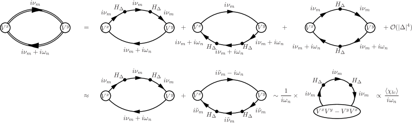
Figure 8: Diagrammatic derivation of the high-frequency small-$\Delta$ limit. The current-current correlator $\pi_{xy}(i\omega_{n})$ is expanded in powers of the pairing Hamiltonian ${H}_{\Delta}$, which is treated as a perturbation. The leading-order contribution in the high-frequency limit comes from the first two terms on the right hand side, as shown in the second line. Note the redefinition of the internal frequency $i\tilde{\nu}_{m}=i\nu_{m}+i\omega_{n}$ in the second term. After the Green’s functions containing the external frequency are factored out, the result is expressed in terms of the expectation value of the loop-current operator $\chi_{lc}$. The double line represents the full Green’s function ${G}$, and the single line denotes the Green’s function ${G}_{0}$ of the normal system.

Keeping only the first two diagrams, therefore, we approximate $\pi_{xy}(i\omega_{n})$ as shown in the second line of Fig. 8. We observe that, in performing the Matsubara summation over the internal frequency, the residue of the poles of the Green’s function containing the external frequency will be at least $\sim 1/\omega^{3}$, whereas the residue of the poles of the other Green’s functions will be $\sim 1/\omega$. Since the $\sim 1/\omega$ contribution only arises from the unit matrix (i.e.  ${\tau}_{0}\otimes{s}_{0}$) component of the Green’s function containing the external frequency, we make the approximation ${G}_{0}({\bm{k}},i\nu_{m}\pm i\omega_{n})\approx(\pm i\omega_{n})^{-1}{\tau}_{0}\otimes{s}_{0}$ and hence factor the external frequency out of the Matsubara sum. This yields the diagram involving the commutator of the velocity vertices and the second-order Green’s function correction ${G_{0}}{H}_{\Delta}{G_{0}}{H}_{\Delta}{G}_{0}$. This product is proportional to the expectation value of the dimensionless loop-current operator Eq. (26) expanded to lowest order in the pairing potential. Evaluating this diagram, we obtain the Hall conductivity

$$\pi_{xy}(i\omega_{n})$$

$$\approx\frac{e^{2}}{\hbar i\omega_{n}}\frac{1}{S\beta}\sum_{{\bm{k}},\nu_{m}}\text{Tr}\{(V^{x}_{\bm{k}}V^{y}_{\bm{k}}-V^{y}_{\bm{k}}V^{x}_{\bm{k}})G_{0}H_{\Delta}G_{0}H_{\Delta}G_{0}\}$$

$$=\frac{e^{2}}{\hbar i\omega_{n}}\frac{1}{\beta}\sum_{\nu_{m}}\int\frac{d^{2}k}{(2\pi)^{2}}\frac{\mu[\bm{v}_{\bm{k}}^{*}\wedge\bm{v}_{\bm{k}}]\,\Xi_{\pm}(\bm{k})}{(\hbar^{2}\nu_{m}^{2}+\epsilon_{\bm{k},1}^{2})(\hbar^{2}\nu_{m}^{2}+\epsilon_{\bm{k},2}^{2})},$$

where $\epsilon_{{\bm{k}},1(2)}=+(-)\sqrt{(\epsilon^{x}_{\bm{k}})^{2}+(\epsilon^{y}_{\bm{k}})^{2}}-\mu$ are the dispersions in the normal state. A similar analysis yields $\pi_{yx}(i\omega_{n})=-\pi_{xy}(i\omega_{n})$. We hence obtain the Hall conductivity

$$\sigma_{H}(\omega)=\frac{2e^{2}}{\hbar\omega^{2}}\frac{1}{\beta}\sum_{\nu_{m}}\int\frac{d^{2}k}{(2\pi)^{2}}\frac{i\mu[\bm{v}_{\bm{k}}^{*}\wedge\bm{v}_{\bm{k}}]\,\Xi_{\pm}(\bm{k})}{(\hbar^{2}\nu_{m}^{2}+\epsilon_{\bm{k},1}^{2})(\hbar^{2}\nu_{m}^{2}+\epsilon_{\bm{k},2}^{2})}\,.$$

We recognize this as the lowest-order term in the expansion of Eq. (40) in powers of the gap magnitude.

References

- (1) M. Sato and Y. Ando, Topological superconductivity: a review. Rep. Prog. Phys. 80, 076501 (2017).
- (2) C. Kallin and J. Berlinsky, Chiral superconductors, Rep. Prog. Phys. 79, 054502 (2016).
- (3) A. J. Leggett, A theoretical description of the new phases of liquid 3He, Rev. Mod. Phys. 47, 331 (1975).
- (4) Andrew P. Mackenzie, Thomas Scaffidi, Clifford W. Hicks, and Yoshiteru Maeno, Even odder after twenty-three years: the superconducting order parameter puzzle of Sr2RuO4, npj Quantum Materials 2, 40 (2017).
- (5) R. Joynt and L. Taillefer, The superconducting phases of UPt3 , Rev. Mod. Phys. 74, 235 (2002).
- (6) J. D. Strand, D. J. Bahr, D. J. van Harlington, J. P. Davis, W. J. Gannon, and W. P. Halperin, The transition between real and complex superconducting order parameter phases in UPt3, Science 328, 1368 (2010).
- (7) Y. Kasahara, T. Iwasawa, H. Shishido, T. Shibauchi, K. Behnia, Y. Haga, T. D. Matsuda, Y. Onuki, M. Sigrist, and Y. Matsuda, Exotic Superconducting Properties in the Electron-Hole-Compensated Heavy-Fermion “Semimetal”, URu2Si2, Phys. Rev. Lett. 99, 116402 (2007).
- (8) M. H. Fischer, T. Neupert, C. Platt, A. P. Schnyder, W. Hanke, J. Goryo, R. Thomale, and M. Sigrist, Chiral -wave superconductivity in SrPtAs, Phys. Rev. B 89, 020509(R) (2014).
- (9) Y. Cao, V. Fatemi, S. Fang, K. Watanabe, T. Taniguchi, E. Kaxiras, and P. Jarillo-Herrero, Unconventional superconductivity in magic-angle graphene superlattices, Nature 556, 43 (2018).
- (10) D. Sa, M. Sardar, and G. Baskaran, Superconductivity in NaxCoOH2O: Protection of a state by spin-charge separation, Phys. Rev. B 70, 104505 (2004); M. L. Kiesel, C. Platt, W. Hanke, and R. Thomale, Model Evidence of an Anisotropic Chiral -Wave Pairing State for the Water-Intercalated NaxCoOH2O Superconductor, Phys. Rev. Lett. 111, 097001 (2013).
- (11) P. M. R. Brydon, L. M. Wang, M. Weinert, and D. F. Agterberg, Pairing of Fermions in Half-Heusler Superconductors, Phys. Rev. Lett. 116, 177001 (2016).
- (12) R. Ganesh, G. Baskaran, J. van den Brink, and D. V. Efremov, Theoretical Prediction of a Time-Reversal Broken Chiral Superconducting Phase Driven by Electronic Correlations in a Single TiSe2 Layer, Phys. Rev. Lett. 113, 177001 (2014).
- (13) N. F. Q. Yuan, K. F. Mak, and K. T. Law, Possible topological superconducting phases of , Phys. Rev. Lett. 113, 097001 (2014).
- (14) Y.-T. Hsu, A. Vaezi, M. H. Fischer, and E.-A. Kim, Topological superconductivity in monolayer transition metal dichalcogenides, Nat. Commun. 8, 14985 (2017).
- (15) A. Kapitulnik, J. Xia, E. Schemm, and A. Palevski, Polar Kerr effect as probe for time-reversal symmetry breaking in unconventional superconductors, New J. Phys. 11, 055060 (2009).
- (16) J. Xia, Y. Maeno, P. T. Beyersdorf, M. M. Fejer, and A. Kapitulnik, High Resolution Polar Kerr Effect Measurements of Sr2RuO4: Evidence for Broken Time-Reversal Symmetry in the Superconducting State, Phys. Rev. Lett. 97, 167002 (2006).
- (17) E. R. Schemm, W. J. Gannon, C. M. Wishne, W. P. Halperin, and A. Kapitulnik, Science 345, 190 (2014).
- (18) E. R. Schemm, R. E. Baumbach, P. H. Tobash, F. Ronning, E. D. Bauer, and A. Kapitulnik, Evidence for broken time-reversal symmetry in the superconducting phase of URu2Si2, Phys. Rev. B 91, 140506(R) (2015).
- (19) E. M. Levenson-Falk, E. R. Schemm, Y. Aoki, M. B. Maple, and A. Kapitulnik, Polar Kerr Effect from Time-Reversal Symmetry Breaking in the Heavy-Fermion Superconductor PrOs4Sb12, Phys. Rev. Lett. 120, 187004 (2018).
- (20) X. Gong, M. Kargarian, A. Stern, D. Yue, H. Zhou, X. Jin, V. M. Galitski, V. M. Yakovenko, and J. Xia, Time-Reversal-Symmetry-Breaking Superconductivity in Epitaxial Bismuth/Nickel Bilayers, Sci. Adv. 3, e1602579 (2017).
- (21) J. Goryo, Impurity-induced polar Kerr effect in a chiral -wave superconductor, Phys. Rev. B 78, 060501(R) (2008).
- (22) R. M. Lutchyn, P. Nagornykh, and V. M. Yakovenko, Frequency and temperature dependence of the anomalous ac Hall conductivity in a chiral superconductor with impurities, Phys. Rev. B 80, 104508 (2009).
- (23) E. J. König and A. Levchenko, Kerr Effect from Diffractive Skew Scattering in Chiral Superconductors, Phys. Rev. Lett. 118, 027001 (2017).
- (24) K. I. Wysokiński, J. F. Annett, and B. L. Györffy, Intrinsic Optical Dichroism in the Chiral Superconducting State of Sr2RuO4, Phys. Rev. Lett. 108, 077004 (2012).
- (25) E. Taylor and C. Kallin, Intrinsic Hall Effect in a Multiband Chiral Superconductor in the Absence of an External Magnetic Field, Phys. Rev. Lett. 108, 157001 (2012).
- (26) M. Gradhand, K. I. Wysokinski, J. F. Annett, and B. L. Györffy, Kerr rotation in the unconventional superconductor Sr2RuO4, Phys. Rev. B 88, 094504 (2013).
- (27) J. Robbins, J. F. Annett, and M. Gradhand, Effect of spin-orbit coupling on the polar Kerr effect in Sr2RuO4, Phys. Rev. B 96, 144503 (2017).
- (28) L. Komendová and A. Black-Schaffer, Odd-Frequency Superconductivity in Sr2RuO4 Measured by Kerr Rotation, Phys. Rev. Lett. 119, 087001 (2017).
- (29) Z. Wang, J. Berlinsky, G. Zwicknagl, and C. Kallin, Intrinsic ac anomalous Hall effect of nonsymmorphic chiral superconductors with an application to UPt3, Phys. Rev. B 96, 174511 (2017).
- (30) R. Joynt and W.-C. Wu, Interband theory of Kerr rotation in unconventional superconductors, Scientific Reports 7, 12968 (2017).
- (31) C. Triola and A. M. Black-Schaffer, Odd-frequency pairing and Kerr effect in the heavy-fermion superconductor UPt3, Phys. Rev. B 97, 064505 (2018).
- (32) G. Baskaran, Resonating-valence-bond contribution to superconductivity in MgB2, Phys. Rev. B 65, 212505 (2002).
- (33) B. Uchoa and A. H. Castro Neto, Superconducting States of Pure and Doped Graphene, Phys. Rev. Lett. 98, 146801 (2007).
- (34) A. M. Black-Schaffer and S. Doniach, Resonating valence bonds and mean-field -wave superconductivity in graphite, Phys. Rev. B 75, 134512 (2007).
- (35) C. Honerkamp, Density Waves and Cooper Pairing on the Honeycomb Lattice, Phys. Rev. Lett. 100, 146404 (2008).
- (36) S. Pathak, V. B. Shenoy, and G. Baskaran, Possible high-temperature superconducting state with a pairing symmetry in doped graphene, Phys. Rev. B 81, 085431 (2010).
- (37) S. Raghu, S. A. Kivelson, and D. J. Scalapino, Superconductivity in the repulsive Hubbard model: An asymptotically exact weak-coupling solution, Phys. Rev. B 81, 224505 (2010).
- (38) T. Ma, Z. Huang, F. Hu, and H.-Q. Lin, Pairing in graphene: A quantum Monte Carlo study, Phys. Rev. B 84, 121410(R) (2011).
- (39) M. L. Kiesel, C. Platt, W. Hanke, D. A. Abanin, and R. Thomale, Competing many-body instabilities and unconventional superconductivity in graphene, Phys. Rev. B 86, 020507(R) (2012).
- (40) R. Nandkishore, L. S. Levitov, and A. V. Chubukov, Chiral superconductivity from repulsive interactions in doped graphene, Nat. Phys. 8, 158 (2012).
- (41) R. Nandkishore and A. V. Chubukov, Interplay of superconductivity and spin-density-wave order in doped graphene, Phys. Rev. B 86, 115426 (2012).
- (42) W. Wu, M. M. Scherer, C. Honerkamp, and K. Le Hur, Correlated Dirac particles and superconductivity on the honeycomb lattice, Phys. Rev. B 87, 094521 (2013).
- (43) Z.-C. Gu, H.-C. Jiang, D. N. Sheng, H. Yao, L. Balents, and X.-G. Wen, Time-reversal symmetry breaking superconducting ground state in the doped Mott insulator on the honeycomb lattice, Phys. Rev. B 88, 155112 (2013).
- (44) A. M. Black-Schaffer, W. Wu, and K. Le Hur, Chiral -wave superconductivity on the honeycomb lattice close to the Mott state, Phys. Rev. B 90, 054521 (2014).
- (45) S. Jiang, A. Mesaros, and Y. Ran, Chiral Spin-Density Wave, Spin-Charge-Chern Liquid, and Superconductivity in -Doped Correlated Electronic Systems on the Honeycomb Lattice, Phys. Rev. X 4, 031040 (2014).
- (46) A. M. Black-Schaffer and C. Honerkamp, Chiral -wave superconductivity in doped graphene, J. Phys.: Condens. Matter 26, 423201 (2014).
- (47) X. Y. Xu, S. Wessel, and Z. Y. Meng, Competing pairing channels in the doped honeycomb lattice Hubbard model, Phys. Rev. B 94, 115105 (2016).
- (48) L.-Y. Xiao, S.-L. Yu, W. Wang, Z.-J. Yao, and J.-X. Li, Possible singlet and triplet superconductivity on honeycomb lattice, Europhys. Lett. 115, 27008 (2016).
- (49) T. Ying and S. Wessel, Pairing and chiral spin density wave instabilities on the honeycomb lattice: a comparative quantum Monte Carlo study, Phys. Rev. B 97, 075127 (2018).
- (50) B. Roy and V. Juričić, Strain-induced time-reversal odd superconductivity in graphene, Phys. Rev. B 90, 041413(R) (2014).
- (51) J. P. L. Faye, P. Sahebsara, and D. Sénéchal, Chiral triplet superconductivity on the graphene lattice, Phys. Rev. B 92, 085121 (2015).
- (52) B. Roy and I. F. Herbut, Unconventional superconductivity on honeycomb lattice: the theory of Kekule order parameter, Phys. Rev. B 82, 035429 (2010).
- (53) F. K. Kunst, C. Delerue, C. M. Smith, and V. Juričić, Kekule versus hidden superconducting order in graphene-like systems: Competition and coexistence, Phys. Rev. B 92, 165423 (2015).
- (54) A. M. Black-Schaffer and K. Le Hur, Topological superconductivity in two dimensions with mixed chirality, Phys. Rev. B 92, 140503(R) (2015).
- (55) J. P. L. Faye, M. N. Diarra, and D. Sénéchal, Kekule superconductivity and antiferromagnetism on the graphene lattice, Phys. Rev. B 93, 155149 (2016).
- (56) Y. Qi, L. Fu, K. Sun, and Z. Gu, Coexistence of antiferromagnetism and topological superconductivity on honeycomb lattice Hubbard model, arXiv:1709.08232.
- (57) C. Xu and L. Balents, Topological superconductivity in twisted multilayer graphene, Phys. Rev. Lett. 121, 087001 (2018).
- (58) M. Fidrysiak, M. Zegrodnik, and J. Spalek, Unconventional topological superconductivity and phase diagram for an effective two-orbital model as applied to twisted bilayer graphene, Phys. Rev. B 98, 085436 (2018).
- (59) H. Guo, X. Zhu, S. Feng, and R.T. Scalettar, Pairing symmetry of interacting fermions on a twisted bilayer graphene superlattice, Phys. Rev. B 97, 235453 (2018).
- (60) C.-C. Liu, L.-D. Zhang, W.-Q. Chen, and F. Yang, Chiral SDW and superconductivity in the magic-angle twisted bilayer-graphene, Phys. Rev. Lett. 121, 217001 (2018).
- (61) Y. Su and S.-Z. Lin, Pairing symmetry and spontaneous vortex-antivortex lattice in superconducting twisted-bilayer graphene: Bogoliubov-de Gennes approach, Phys. Rev. B 98, 195101 (2018).
- (62) F. Wu, Topological Chiral Superconductor with Spontaneous Vortices and Supercurrent in Twisted Bilayer Graphene, arXiv:1811.10620.
- (63) F. D. M. Haldane, Model for a quantum Hall effect without landau levels: Condensed-matter realization of the “parity anomaly”, Phys. Rev. Lett. 61, 2015 (1988).
- (64) G. W. Semenoff, Condensed-Matter Simulation of a Three-Dimensional Anomaly, Phys. Rev. Lett. 53, 2449 (1984).
- (65) Y. Yanase, Nonsymmorphic Weyl superconductivity in UPt3 based on representation, Phys. Rev. B 94, 174502 (2016).
- (66) B. A. Bernevig and T. L. Hughes, Topological Insulators and Topological Superconductors (Princeton University Press, Princeton, 2013).
- (67) More complicated bilinear products of and may also involve , but we focus on the simplest case of in our paper.
- (68) M. Sigrist and K. Ueda, Phenomenological theory of unconventional superconductivity, Rev. Mod. Phys. 63, 239 (1991).
- (69) P. M. R. Brydon, D. F. Agterberg, H. Menke, and C. Timm, Bogoliubov Fermi surfaces: General theory, magnetic order, and topology, Phys. Rev. B 98, 224509 (2018).
- (70) A. Ramires and M. Sigrist, Identifying detrimental effects for multiorbital superconductivity: Application to , Phys. Rev. B 94, 104501 (2016).
- (71) A. Ramires, D. F. Agterberg, and M. Sigrist, Tailoring by symmetry principles: The concept of superconducting fitness, Phys. Rev. B 98, 024501 (2018).
- (72) V. P. Mineev, Whether there is the intrinsic Hall effect in a multi-band superconductor?, J. Phys. Soc. Japan 81, 093703 (2012).
- (73) S. Tewari, C. Zhang, V. M. Yakovenko, and S. Das Sarma, Time-reversal symmetry breaking by a () density-wave state in underdoped cuprate superconductors, Phys. Rev. Lett. 100, 217004 (2008).
- (74) B. S. Shastry, B. I. Shraiman, and R. P. P. Singh, Faraday rotation and the Hall constant in strongly correlated Fermi systems, Phys. Rev. Lett. 70, 2004 (1993).
- (75) E. Lange and G. Kotliar, Magneto-optical Sum Rules Close to the Mott Transition, Phys. Rev. Lett. 82, 1317 (1999).
- (76) T. A. Bojesen, E. Babaev, and A. Sudbø, Time reversal symmetry breakdown in normal and superconducting states in frustrated three-band systems, Phys. Rev. B 88, 220511(R) (2013); Phase transitions and anomalous normal state in superconductors with broken time-reversal symmetry, Phys. Rev. B 89, 104509 (2014).
- (77) D. F. Agterberg, D. S. Melchert, and M. K. Kashyap, Emergent loop current order from pair density wave superconductivity, Phys. Rev. B 91, 054502 (2015); Y. Wang, D. F. Agterberg, and A. Chubukov, Interplay between pair- and charge-density-wave orders in underdoped cuprates, ibid, 115103 (2015).
- (78) J. F. Dodaro, S. A. Kivelson, Y. Schattner, X. Q. Sun, and C. Wang, Phases of a phenomenological model of twisted bilayer graphene, Phys. Rev. B 98, 075154 (2018).
- (79) N. F. Q. Yuan and L. Fu, Model for the metal-insulator transition in graphene superlattices and beyond, Phys. Rev. B 98, 045103 (2018).
- (80) M. Koshino, N. F. Q. Yuan, T. Koretsune, M. Ochi, K. Kubo, and L. Fu, Maximally Localized Wannier Orbitals and the Extended Hubbard Model for Twisted Bilayer Graphene, Phys. Rev. X 8, 031087 (2018).
- (81) J. Kang and O. Vafek, Symmetry, Maximally Localized Wannier States, and a Low-Energy Model for Twisted Bilayer Graphene Narrow Bands, Phys. Rev. X 8, 031088 (2018).
- (82) H. C. Po, L. Zou, A. Vishwanath, and T. Senthil, Origin of Mott Insulating Behavior and Superconductivity in Twisted Bilayer Graphene, Phys. Rev. X 8, 031089 (2018).
- (83) S. K. Ghosh, J. F. Annett, and J. Quintanilla, Time-reversal symmetry breaking in superconductors through loop Josephson-current order, arXiv:1803.02618.
- (84) This relation is obtained by interchanging fermion operators in the pairing terms of Eq. (44) and then changing the variable of summation from to . It is known as in the context of odd-frequency pairing (see J. Linder and A. V. Balatsky, arXiv:1709.03986), which is not considered in our paper.
- (85) A similar structure of for spin 3/2 is discussed by D. F. Agterberg, P. M. R. Brydon, and C. Timm, Bogoliubov Fermi surfaces in superconductors with broken time-reversal symmetry, Phys. Rev. Lett. 118, 127001 (2017).