Constraining Type Ia Supernova Progenitor Scenarios with Extremely Late-time Photometry of Supernova SN 2013aa

Abstract

We present Hubble Space Telescope observations and photometric measurements of the Type Ia supernova (SN Ia) SN 2013aa 1500 days after explosion. At this epoch, the luminosity is primarily dictated by the amounts of radioactive ${}^{57}\textrm{Co}$ and ${}^{55}\textrm{Fe}$, while at earlier epochs, the luminosity depends on the amount of radioactive ${}^{56}\textrm{Co}$. The ratio of odd-numbered to even-numbered isotopes depends significantly on the density of the progenitor white dwarf during the SN explosion, which, in turn, depends on the details of the progenitor system at the time of ignition. From a comprehensive analysis of the entire light curve of SN 2013aa, we measure a $M({}^{57}\textrm{Co})/M({}^{56}\textrm{Co})$ ratio of $0.02^{+0.01}_{-0.02}$, which indicates a relatively low central density for the progenitor white dwarf at the time of explosion, consistent with double-degenerate progenitor channels. We estimate $M({}^{56}\textrm{Ni})=0.732\pm 0.151\>\mathrm{M_{\odot}}$, and place an upper limit on the abundance of ${}^{55}\textrm{Fe}$. A recent study reported a possible correlation between $M({}^{57}\textrm{Co})/M({}^{56}\textrm{Co})$ and stretch for four SNe Ia. SN 2013aa, however, does not fit this trend, indicating either SN 2013aa is an extreme outlier or the correlation does not hold up with a larger sample. The $M({}^{57}\textrm{Co})/M({}^{56}\textrm{Co})$ measured for the expanded sample of SNe Ia with photometry at extremely late times has a much larger range than that of explosion models, perhaps limiting conclusions about SN Ia progenitors drawn from extremely late-time photometry.

1 Introduction

Type Ia Supernova (SNe Ia) are the result of a thermonuclear explosion of a carbon-oxygen white dwarf (WD) in a binary system (Hoyle & Fowler 1960; Colgate & McKee 1969; Woosley & Weaver 1986). While the applications of SNe Ia as standardizable candles are far reaching in the realm of cosmology (e.g., Riess et al. 1998; Perlmutter et al. 1999), the exact nature of the explosion and the progenitor system, and in particular the binary companion, are still an open question (see e.g., Maoz et al. 2014).

There are several ways to potentially produce a SN Ia (Woosley et al. 1986). In these models, the (primary) WD is usually either very close to the Chandrasekhar mass, having undergone a simmering stage (Piro & Bildsten 2008; Piro & Chang 2008) and having a high central density, or below the Chandrasekhar mass with a lower central density (Iben & Tutukov 1984; Woosley et al. 2004). The details of the explosive nuclear burning depends critically on the central density. In particular, explosions with higher central densities will produce more Fe-group elements with an odd number of nucleons (Iwamoto et al. 1999; Seitenzahl et al. 2013a). While other aspects of the explosion have a larger effect on the amount of odd-numbered, radioactive isotopes produced (e.g., metallicity or M(⁵⁶Ni)), measuring the mass of these isotopes can distinguish explosion models.

In addition to different explosions, there are fundamentally different progenitor channels for SNe Ia. The single-degenerate (SD) and double-degenerate (DD) channels, which have non-degenerate and WD companion stars, respectively. The DD channel will naturally have a sub-Chandrasekhar mass primary and a relatively low central density (Pakmor et al. 2010, 2011). While some SD systems might result in a sub-Chandrasekhar mass explosion, the classical model involves a Chandrasekhar-mass WD and a high central density (Khokhlov 2000; Han & Podsiadlowski 2004).

The single-degenerate (SD) model argues that the explosion is triggered by a high central density, delayed detonation of a near-Chandrasekhar-mass WD as it accretes material and energy from main-sequence or larger star (Whelan & Iben 1973, Khokhlov 1991). Alternatively, the double-degenerate (DD) model consists of a low central density, violent merger of two, sub-Chandrasekhar-mass WD stars (Webbink 1984, Pakmor et al. 2012). While both are accepted theoretical predictions, the direct detection of the progenitor system is difficult, with most DD models leaving no post-explosion indication of the system responsible. There have, however, been recent constraints placed on the direct detection of progenitor systems following SD models (Chomiuk et al. 2016, Maguire et al. 2016). Fortunately, other methods of progenitor system constraint come from the unique modeling of these explosions by Röpke et al. (2012) and Seitenzahl et al. (2013b), all of which are verifiable via the study of radioactive decay in late-time bolometric light curves of SNe Ia.

By Arnett’s Law, the bolometric luminosity produced at peak magnitude is proportional to the rate of energy deposition by the radioactive decay chain $\ce{{}^{5}6Ni->[t_{1/2}=6.08\textrm{d}]{}^{5}6Co->[t_{1/2}=77.2\textrm{d}]{}^{5}6Fe}$ (Arnett 1982). While Arnett’s Law is an approximation, the decay of ${}^{56}\textrm{Ni}$ remains the most prominent source of heating in SNe Ia and produces primarily $\gamma$-rays and positrons, whose energies are deposited and thermalized in the expanding ejecta (Seitenzahl & Townsley 2017). Not only can the total mass of ${}^{56}\textrm{Ni}$ be determined from the peak luminosity, the isotopic yields generated in decay chains ${}^{57}\textrm{Co}\rightarrow{}^{57}\textrm{Fe}$ and ${}^{55}\textrm{Fe}\rightarrow{}^{55}\textrm{Mn}$ can be indirectly detected from the light curve evolution of SNe Ia at epochs $>300$ days after explosion (Seitenzahl et al. 2009). Model analysis has shown that the mass ratios of these nucleosyntheic yields differ between single and double degenerate explosion models, thus making them extremely useful in identifying the pre-explosion SNe Ia progenitor systems (Röpke et al. 2012).

Testing each model requires precise photometric data from continuous observations of nearby SNe Ia $>400$ days after peak luminosity. This is a challenging effort due to the variability of SNe Ia explosions coupled with the ability to perform accurate photometric measurements at late enough epochs to detect the radioactive decay of isotopes other than ${}^{56}\textrm{Ni}$. Nonetheless, a few significant studies have been recently performed on SNe Ia in close proximately to us and with multiple broad band photometric detections produced at late epochs.

SN 2011fe remains to be one of the most highly studied late-time SNe Ia, with numerous examinations of radioactive decay channels since its nearby discovery (Kasen & Nugent 2013). Shappee et al. (2017) were able to detect abundances of ${}^{56}\textrm{Co}$ and ${}^{57}\textrm{Co}$ as well as place an upper limit on the mass of ${}^{55}\textrm{Fe}$, while indicating that the fits to the data preferred a DD explosion model. A similar study by Dimitriadis et al. (2017) examined the near infrared contribution to the bolometric luminosity of SN 2011fe, but found a contradicting alignment to the single-degenerate explosion model of a high central density white dwarf star.

Further examinations of extremely late-time supernovae also make predictions of the pre-explosion progenitor system. Graur et al. (2016) finds a distinct detection of ${}^{57}\textrm{Co}$ in the light curve of SN 2012cg and predicts a single-degenerate explosion mechanism. The analysis of SN 2014J makes similar conclusions in their determination of mass ratios that prefer a high central density explosion model (Yang et al. 2017). Alternatively, the mass ratio found in SN 2015F by Graur et al. (2017) shows evidence for a double degenerate merger of two white dwarfs. Graur et al. (2017) also examines the relationship between the calculated light curve stretch and ${}^{57}\textrm{Co}$/${}^{56}\textrm{Co}$ in all four late-time SNe Ia, the implications of which we will discuss as it relates to SN 2013aa.

The detection of SN 2013aa at a phase of $\sim 1500$ days presents a unique opportunity to examine the nucleosynthetic yields of late-time decay. SN 2013aa is the fifth SNe Ia to be observed at an epoch $>1000$ days, with a photometric detection at the second latest phase next to SN 2011fe. The measured late-time bolometric luminosity, combined with early-time data, allows for a fitted calculation of radionuclide abundances powering the light curve. The mass ratios of ${}^{56}\textrm{Co}$, ${}^{57}\textrm{Co}$, and ${}^{55}\textrm{Fe}$ found in SN 2013aa can then compared with explosion models as an indicator of the progenitor system. With only four recorded late-time SNe Ia prior to SN 2013aa, this analysis will contribute to the understanding of late-time trends in the light curves of SNe Ia.

In Section 2 we present observations and data reduction of SN 2013aa. In Section 3 we discuss the calculation of radioactive isotope abundances. In Section 4 we examine the implications of measured mass ratios in the context of explosion models and other late-time studies.

2 Observations

In this section, we briefly introduce SN 2013aa, presenting the published photometric and spectroscopic data and basic parameters from early-time data. We also present late-time HST photometry.

2.1 Early-time data (up to 400 days)

SN 2013aa was discovered by the Backyard Observatory Supernova Survey (BOSS) on 2013 February 13 (Parker et al. 2013) and confirmed to be a SN Ia on 2013 February 16 (Parrent et al. 2013). SN 2013aa is located in the barred spiral galaxy NGC 5643, 74^′′ West and 180^′′ South from the galactic center (Graham et al. 2017). Another SN Ia, SN 2017cbv, is in the same galaxy, providing an independent distance estimate to SN 2013aa (Shappee et al., in preparation). Applying the SALT2 algorithm (Guy et al. 2007) to the SN 2017cbv data, we determine that the distance to NGC 5643 is $13.95\pm 0.35$ Mpc, corresponding to a distance modulus of $\mu=30.72\pm 0.05$ mag. Primary parameters of SN 2013aa and its host galaxy, NGC 5643, are reported in Table 1.

Table 1: Main Parameters of SN 2013aa and Host Galaxy

Host Galaxy									NGC 5643
Galaxy Type									SAB(rs)c
Redshift									$0.003999\pm 0.000007$
Distance									$13.95\pm 0.3$ Mpc
Distance Modulus, $\mu$									$30.72\pm 0.05$ mag
$\textrm{RA}_{\textrm{SN}}$									$14^{\textrm{h}}32^{\textrm{m}}33.919^{\textrm{s}}$
$\textrm{Dec}_{\textrm{SN}}$									$-44^{\circ}13^{\prime}28.763^{\prime\prime}$
Stretch									1.072 $\pm$ 0.014
$m_{B}^{\mathrm{peak}}$									$11.11\pm 0.05$ mag
$M_{B}^{\mathrm{peak}}$									$-19.49\pm 0.07$ mag

SN 2013aa was initially followed by the Las Cumbres Observatory Global Telescope (LCOGT) Supernova Key Project (Brown et al. 2013), with the $B\!V\!gri$ light curves first published by Graham et al. (2017). As mentioned in Graham et al. (2017), most of the near-peak photometry was saturated, thus we complement the early-time light curve with optical ($U\!B\!V$) data from the Swift Optical/Ultraviolet Supernova Archive (SOUSA; Brown et al. 2014). This data provides adequate coverage of the SN from $-10$ to $\sim$200 days after peak. Additionally, Graham et al. (2017) present $gri$ photometry from the Gemini Multi-Object Spectrograph (GMOS; Davies et al. 1997), at $\sim$400 days. In Fig. 1, we present the early-time ($-15$ to 50 days from peak) light curves of SN 2013aa.

We fit the light curves with sifto (Conley et al. 2008), with which we recover a time of maximum light of $\mathrm{MJD_{max}}=56342.69\pm 0.18$, peak brightnss of $m_{B}^{\mathrm{peak}}=11.11\pm 0.05$ mag, peak color of $(B-V)_{0}=-0.03\pm 0.05$ mag and a stretch of $s=1.072\pm 0.014$. Restricting our fit to only the Swift photometry, which covers the peak of the light curve, we calculate $s=1.067\pm 0.023$, consistent with what was found using all available data.

Adopting the distance modulus from SN 2017cbv, $\mu=30.72\pm 0.05$ mag, SN 2013aa had a $B$-band absolute magnitude at peak of $M_{B}^{\mathrm{peak}}=-19.49\pm 0.07$ mag. The relatively high peak absolute magnitude is consistent with its slightly broad light curves.

A collection of SN 2013aa spectra is presented in Fig. 2, spanning from 32 to 398 days after peak. These spectra have been published by Childress et al. (2015) and Graham et al. (2017). All the spectra were retrieved through the WISeREP archive (Yaron & Gal-Yam 2012).

We used the Supernova Identification package (SNID; Blondin & Tonry 2007) and Superfit (Howell et al. 2005) at the earliest spectrum (32.3 days after peak) to sub-classify the SN. Both packages reported SN 1991T-like objects as having the best-matching spectra in accordance with the early-time light-curve evolution. However, SN 1991T-like objects are difficult to distinguish from lower-luminosity SNe Ia a month after peak, and the sub-classification is somewhat uncertain. With this in mind, throughout this paper, we will consider SN 2013aa as a normal-to-overluminous SNe Ia.

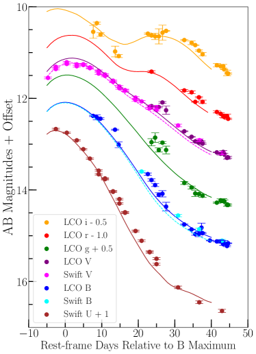
Figure 1: LCOGT and Swift light curves of SN 2013aa around peak. LCOGT photometry in shown as B (blue), V (purple), g (green), r (red) and i (orange). Swift photometry shown as U (brown), B (cyan) and V (magenta). The photometry has been corrected for MW extinction. Solid and dashed lines are the sifto fits on the LCOGT and Swift photometry respectively.

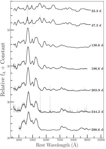
Figure 2: Spectra of SN 2013aa. Raw spectra are shown in gray, smoothed spectra with black lines.

2.2 HST Data

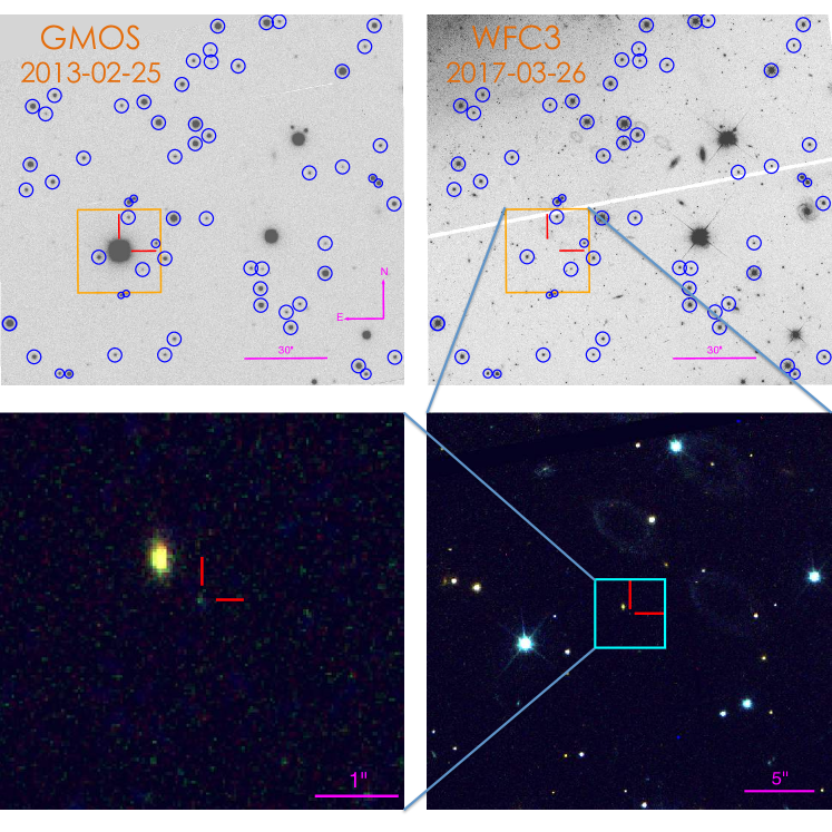
Figure 3: Top Images: Explosion image taken by Gemini with GMOS (left). HST image of SN 2013aa at 1500 day epoch taken with WFC3. Stars used for astrometric solution circled in blue. Bottom Images: HST RGB images centered on SN 2013aa with $30^{\prime\prime}$ (right) and $5^{\prime\prime}$ (left) radii from the source.

Due to its distance and significant offset from its host galaxy, SN 2013aa is an excellent target for late-time observations. Under HST program DD–14925 (Foley 2016), we imaged SN 2013aa ($\alpha=14^{\textrm{h}}32^{\textrm{m}}33.919^{\textrm{s}},\delta=-44^{\circ}13^{\prime}28.763^{\prime\prime}$) on 2017 March 22, 24, 26 & 30 with the HST Wide Field Camera 3 (WFC3). These observations were obtained in parallel with STIS observations of SN 2017cbv. The source was observed with wide-band filters F350LP, F555W, and F814W at varying exposures times. Photometric measurements are reported in Table 2.

We received HST WFC3 image files in the FLC format, all of which have been corrected for dark current, flat fielding, and charge transfer efficiency through the HST calibration pipeline. We used the IRAF package StarFind to located reference stars for initial frame alignment. We performed fine alignment of all images to one-another using calibration algorithm TweakReg. With all frames aligned, we ran the AstroDrizzle reduction package (Gonzaga & et al. 2012) for cosmic ray removal and generation of median and drizzled science images for each HST filter used. We constructed a drizzled template image of all HST filters by overlaying each frame, which was then used as reference during photometric calculations.

To determine the position of SN 2013aa in the WFC images, we determined a geometric transformation between the HST images and Gemini images taken when the SN was brighter. Using 21 stars common to each image and the Gaia stellar catalog, we calculated a WCS solution for both HST and Gemini images. We aligned the WCS of the HST image to that of Gemini based on 72 common, unsaturated stars. We then determine the position of SN 2013aa in the HST images.

We determined the positional systematic uncertainty related to our geometric transformation by performing the transformation many times using a bootstrap re-sampling (with replacement). The final positional uncertainty is a combination of the systematic uncertainty, the statistical uncertainty of the geometric transformation, and the statistical uncertainty from centroiding the SN.

Our best estimate of the position of SN 2013aa is $\alpha=14^{\textrm{h}}32^{\textrm{m}}33.919^{\textrm{s}}\ \pm 0.003^{\textrm{s}},\ \delta=-44^{\circ}13^{\prime}28.76^{\prime\prime}\ \pm 0.03^{\prime\prime}$. Images of SN 2013aa with reference stars are displayed in Figure  3. We detected a point source in our HST image that was $+0.01^{\prime\prime}$ East and $+0.01^{\prime\prime}$ North of the supernova position found in the Gemini explosion image. This translates to a $0.31\sigma$ offset in Right Ascension and a $0.33\sigma$ offset in Declination. The position of the sources in both HST and Gemini images agree with one another, which suggests that they are in fact the same source.

We performed Point Spread Function (PSF) photometry with DOLPHOT (Dolphin 2000) on the F350LP, F555W, and F814W images. DOLPHOT ran simultaneously on all frames while using the combined template HST frame for reference. We used default WFC3 DOLPHOT parameters in the input file, keeping the sigPSF value (minimum signal-to-noise for a PSF calculation) at 10. Using 52 PSF stars in the photometric solution, we detected a point source in all three filter frames that was within the uncertainties of the astrometric solution, confirming that this was indeed SN 2013aa. The source is shown most clearly in the bottom panel of Figure 3.

In this DOLPHOT detection, we measure the apparent magnitudes of SN 2013aa to be $27.969\pm 0.082$ in F350LP, $27.971\pm 0.280$ in F555W, and $27.465\pm 0.177$ in F814W, corresponding to signal-to-noise ratios of 13.3, 3.9, and 6.1, respectively. The brightness of this source is similar to that expected for a SN 2013aa at this epoch. We calibrated our apparent magnitudes from DOLPHOT to AB magnitudes using the WFC3/UVIS2 photometry zeropoint tables given by the Space Telescope Science Institute (STSci). As a result of the default aperture correction performed by DOLPHOT during the photometry calculation process, we applied the infinite aperture zeropoint values to our generated absolute magnitudes.

Table 2: Photometric Observations

MJD	Band	Exp. Time	AB Maga	Telescope
		(s)
57834 - 57842	350LP	507 - 537	27.969 (0.082)	HST/WFC3
57834 - 57842	555W	507-537	27.971 (0.280)	HST/WFC3
57834 - 57842	814W	1014-1074	27.465 (0.177)	HST/WFC3

Note. — Exposures were taken on 2017 March 22, 24, 26, and 30. All four days of observations were combined into a single image for each respective filter.

To determine the chance coincidence between SN 2013aa and our identified source, we look at other detected objects within a $5^{\prime\prime}$ radius of SN 2013aa. We limit the sample of reasonable objects to have ${\rm S/N}\geq 5$, be classified as a star by Dolphot (type 1 or 2), have a roundness of $<$0.5 (as determined by Dolphot), have a sharpness between $-0.3$ and 0.3, and have a Dolphot photometric quality flag of 0 or 1. We find 10 reasonable objects with a $5^{\prime\prime}$ radius, resulting in a chance coincidence of only 0.2%.

3 Analysis

In this section we briefly detail how we generated a pseudo-bolometric light curve from the photometric data described in Section 2. We then discuss our analysis of different elemental decay chains responsible for light curve shape and the process of determining each radioactive isotope mass based on the fit to our bolometric luminosity data.

3.1 Constructing a pseudo-bolometric light curve

In order to construct the pseudo-bolometric light curve of SN 2013aa, we employ similar techniques as performed for other late-time SN Ia studies, that includes the modification of the SN spectra to match a series of photometric observations and, subsequently, integration of these modified spectra over the optical wavelengths (e.g., Graur et al. 2016; Dimitriadis et al. 2017; Graur et al. 2017; Kerzendorf et al. 2017; Shappee et al. 2017). We correct all photometric data, both ground- and space based, for Milky Way Extinction according to Cardelli et al. (1989) with $R_{v}=3.1$, and find no host-galaxy extinction to correct for in the data.

For photometric epochs with phases of $\sim$100 to 200 days, we mangle (Hsiao et al. 2007) the closest-in-time spectrum to the LCOGT photometric data. For the $\sim$400-day epoch, we perform the same operation with the GMOS photometry and spectrum. For the 1500-day photometric epoch, there is no spectrum of SN 2013aa or any other SN Ia; instead, we use a 1000-day spectrum of SN 2011fe (Taubenberger et al. 2015). The bolometric flux is computed by integrating each modified synthetic spectrum from 4000 to 9000 Å, obtaining errors by Monte Carlo re-sampling of the observed photometry. Finally, we calculate the optical bolometric luminosity by scaling the integrated flux with the distance to the SN, estimated in Section 2.1.

The choice of wavelength range for generating the pseudo-bolometric light curve was set by the wavelength coverage of the available spectra, and in particular the GMOS spectrum (see Fig. 2). While this wavelength range is narrower than pseudo-bolometric light curves generated for other SNe Ia (usually $\sim$3500–10000 Å), the dominant spectral lines of SNe Ia at these phases, mainly from iron peak elements and Ca II, are included in our wavelength range. We can estimate the fraction of flux lost bluewards (3500–4000 Å) and redwards (9000–10000 Å) of our pseudo-bolometric wavelength range by using spectra of the well-observed SN 2011fe: we calculate a fraction of 5% and 9% at 348d, reducing to 4% and 7% at 1034d. Our closest spectrum to the GMOS spectrum at 398d is the WiFeS spectrum at 344d, which spans from 3500–9280Å, for which we estimate a fraction of flux lost bluewards (i.e. the integrated flux from 3500–4000 over the integrated flux from 3500–9280Å) and redwards (i.e. the integrated flux from 9000–9280 over the integrated flux from 3500–9280Å) of our pseudo-bolometric wavelength range to be 1.2% and 1.5% respectively. By using spectra of the well-observed SN 2011fe, which cover a wider wavelength range (3000–10000Å), the equivalent blueward-redward flux losses are 5% and 9% at 348, reducing to 4% and 7% at 1034d.

3.2 The bolometric light curve model

Figure 4: Left: Bolometric luminosities of SN 2013aa with respect to SD (orange) and DD (purple) explosion models using fractions of ${}^{56}\textrm{Co}$ predicted by Röpke et al. (2012). Blue line is calculated from the expected mass of ${}^{57}\textrm{Co}$ based on fit for ${}^{57}\textrm{Co}$ / ${}^{56}\textrm{Co}$ versus stretch shown by Graur et al. (2017). This trend is plotted in Figure 5. Right: Our three separate fits to bolometric data. Values found for ${}^{56}\textrm{Co}$, ${}^{57}\textrm{Co}$, and ${}^{55}\textrm{Fe}$ reported in Table 3. Other three lines represent the decomposition of ${}^{56}\textrm{Co}$, ${}^{57}\textrm{Co}$, and ${}^{55}\textrm{Fe}$ decay chains using the masses found in Fit 2 as well as the upper limit of $M({}^{55}\textrm{Fe})$ measured in Fit 1.

The light curve of a SN Ia is powered by the thermalization of the expanding ejecta due to the deposition of energy from the radioactive decay of several decay chains. At early times, the dominant contribution comes from ${}^{56}\textrm{Ni}$, the most abundant synthesized element, and its daughter isotope, ${}^{56}\textrm{Co}$, with its decay channel $\ce{{}^{5}6Co->[t_{1/2}=77.2\textrm{d}]{}^{5}6Fe}$ being the most important for epochs up to 2 yrs after explosion. At later times, and as the column density of the expanding ejecta decreases, additional energy is deposited by the radioactive decays of $\ce{{}^{5}7Co->[t_{1/2}=271.2\textrm{d}]{}^{5}7Fe}$ and ^55Fe -¿[ t_1/2=999.67 d ] ^55Mn . All of these decay chains produce $\gamma$-rays, X-rays and charged leptons (positrons, Auger electrons, and internal conversion electrons). In our analysis we employ the same decay energies and constants as presented in Table 2 of Seitenzahl et al. (2014). In this framework, the luminosity produced can be approximated by the Bateman equation:

$$\begin{split}&L_{A}(t)=2.221\frac{\lambda_{A}}{A}\frac{M(A)}{M_{\odot}}\frac{q^{x}_{A}+q^{l}_{A}f^{l}_{A}(t)+q^{\gamma}_{A}f^{\gamma}_{A}(t)}{\mathrm{keV}}\\ &\ \ \ \ \ \ \ \ \ \ \ \ \ \ \ \ \ \ \ \ \ \ \ \ \ \ \ \ \ \ \textrm{exp}(-\lambda_{A}t)\ \times\ \ 10^{43}\ \textrm{erg}\ \textrm{s}^{-1}\end{split}$$ (1)

where $t$ is time since explosion, $\lambda_{A}$ is the decay constant, $A$ is the atomic number, and $q^{l}$, $q^{\gamma}$, and $q^{x}$ are the average energies of charged leptons, $\gamma$-rays, and X-rays, respectively, per decay. In this equation, $f^{\gamma}_{A}(t)$ and $f^{l}_{A}(t)$ describe the trapping of the deposited energy of the $\gamma$-rays and charged leptons respectively, and, assuming homologous expansion, are given by

$$f^{\gamma,l}_{A}=1-\textrm{exp}\Big{[}-\Big{(}\frac{t^{\gamma,l}_{A}}{t}\Big{)}^{2}\Big{]}$$ (2)

In previous late-time studies, such as Graur et al. (2016), Shappee et al. (2017) and Graur et al. (2017), with late-time data $>500$ days, the authors consider only the charged leptons deposited energy, for which they assume complete trapping in the decay of ${}^{56}\textrm{Co}$ (i.e., $f^{l}_{A}=1$), and no positron trapping in the decays of ${}^{57}\textrm{Co}$ and ${}^{55}\textrm{Fe}$ (i.e., $f^{l}_{A}=0$). For the ${}^{56}\textrm{Co}$ $\gamma$-rays, a timescale of $t^{\gamma}_{56}\approx 35$ days was found to fit the late-time light curves of several SNe Ia (Sollerman et al. 2004; Stritzinger & Sollerman 2007; Leloudas et al. 2009; Zhang et al. 2016) While these SNe Ia do have lower predicted mass of ${}^{56}\textrm{Ni}$ than SN 2013aa, the application of $t^{\gamma}_{56}\approx 35$ days is still an adequate assumption and has no effect on the analysis.

While Equation 1 describes the bolometric luminosity (that is, the complete energetic output across the electromagnetic spectrum), the photometric data presented here and in (most of) the aforementioned studies are primarily optical data, with some cases including near-infrared observations. A common approach is to assume that the optical luminosity scales with the complete bolometric one as $L_{\rm opt}(t)=B(t)\times L_{\rm bol}(t)$, where $B(t)$ is the fraction of the bolometric luminosity in the optical and is often assumed to be a constant in time. In this sense, 1/$B(t)$ resembles a “bolometric correction”, i.e. a function that transforms the optical flux to a bolometric one. We can estimate $B(t)$ by calculating the ratio between the ${}^{56}\textrm{Co}$ mass found by fitting the late-time data with Equation 1 over the total ${}^{56}\textrm{Ni}$ mass as determined from data around peak (where ${}^{56}\textrm{Ni}$ dominates), for which the non-optical contribution at this phase is $\leq$15% (e.g. see Pereira et al. 2013, for SN 2011fe). Values of $B(t)$ calculated by Graur et al. (2017) for a sample of SNe Ia with late-time data range from 20-40%. However, Dimitriadis et al. (2017) showed that, for SN 2011fe, a non-constant $B$ can explain the increase of the late-time non-optical contribution, approximating the optical contribution with a sigmoid function:

$$B(t)=1-\frac{P_{0}}{1-e^{P_{1}\times(t-P_{2})}}$$ (3)

In that work, this non-optical contribution, consisting of the $J\!H\!K$ near-infrared bands, increases from $\sim$5 to 35%, from 200 to 600 days after the $B$-band maximum brightness. This effect can be seen as a faster decline of the (optical bolometric) light curve at these epochs, compared to the expected radioactive decay slope, predicted by known radioactive decay chains. The physical origin of this faster decline remains elusive: positron escape models, a re-distribution of optical flux to the mid/far-infrared Fransson & Jerkstrand (2015) or time-dependent effects, such as freeze-out could provide an explanation.

3.3 Results from Light-Curve Model Fitting

Table 3: Model Fit to Pseudo-Bolometric Light Curve Data

Model	${}^{56}\textrm{Co}$	${}^{57}\textrm{Co}$	${}^{55}\textrm{Fe}$	$t^{\gamma}_{56}$	$t^{l}_{56}$	$\chi^{2}$	DOF
	$(\textrm{M}_{\odot})$	$(\textrm{M}_{\odot})$	$(\textrm{M}_{\odot})$	(days from explosion)	(days from explosion)
Fit 1	$0.589^{+0.014}_{-0.014}$	$0.00002^{+0.0001}_{-0.00002}$	$0.006^{+0.001}_{-0.006}$	$35^{a}$	-	298.4	23
Fit 2	$0.631^{+0.015}_{-0.015}$	$0.006^{+0.001}_{-0.006}$	$0.0002^{+0.0007}_{-0.0002}$	$35^{a}$	$281.02^{+16.44}_{-15.29}$	20.4	22
Fit 3	$0.732^{a}$	$0.015^{+0.0075}_{-0.015}$	$0.0000007^{+0.000007}_{-0.0000007}$	$35^{a}$	-	21.3	20
Fit 4	$0.59^{+0.01}_{-0.01}$	$0.006^{+0.001}_{-0.001}$	$0^{a}$	$35^{a}$	-	299.7	24

In this work, we will explore four models for the late-time light curve of SN 2013aa: (1) Complete positron trapping (i.e., $f^{l}_{A}=1$ & negligible $t^{l}_{55,56,57}$) and free-streaming $\gamma$-rays at late-times (i.e., $f^{\gamma}_{55,57}=0$ & negligible $t^{\gamma}_{55,57}$) , (2) the same as 1, but with possible positron escape, for which we will assume a same form of $f^{l}_{A}$ as the trapping function of the $\gamma$-rays (i.e., as in Equation 2), (3) the same as 1, but with a time-dependent non-optical contribution (Equation 3), and (4) the same as 1, but with no ${}^{55}\textrm{Fe}$, as was assumed by Graur et al. (2017). For all of our fits, we assume $t^{\gamma}_{56}=35$ days, and, by applying a Markov-Chain Monte-Carlo fitting algorithm, determine the amount of ${}^{56}\textrm{Co}$, ${}^{57}\textrm{Co}$, and ${}^{55}\textrm{Fe}$. In our analysis, we use emcee, a Python-based application of an affine invariant MCMC with an ensemble sampler (Foreman-Mackey et al. 2013). Working with an MCMC allows for the detection of degeneracy amongst free variables that could not be properly identified with a standard $\chi^{2}$ fitting algorithm. Unfortunately, SN 2013aa has no data between 400 and 1500 days. As a result, it is difficult to separate the contributions of ${}^{57}\textrm{Co}$ and ${}^{55}\textrm{Fe}$ to the late-time light curve. However, the current data are still constraining for explosion models.

An important step in consistently comparing our late-time mass estimates of the different scenarios considered, is an accurate determination of the total ${}^{56}\textrm{Ni}$ mass, synthesized in the explosion. At early times, the luminosity is dominated by the ${}^{56}\textrm{Ni}$ decay and almost all of the light is emitted in the optical (e.g., Pereira et al. 2013). In the sample study of Graur et al. (2017), the authors estimate the ${}^{56}\textrm{Ni}$ mass by fitting a straight line to the $M_{56}$ values of Childress et al. (2015) over their sifto stretch values. A similar calculation for SN 2013aa yields $M_{56}=0.732\pm 0.151$ M_⊙. As a consistency check, we additionally estimate the ${}^{56}\textrm{Ni}$ mass from the bolometric luminosity at peak, following the widely-used Arnett law Arnett (1982). Using our early-time photometry (Section 2.1) and a template SN Ia spectrum from Hsiao et al. (2007) at peak, we integrate the spectrum and estimate $L_{peak}=1.56\pm\>0.05\times 10^{43}\>\mathrm{erg\>s^{-1}}$. Assuming a rise time of 17 days, we estimate $M_{56}=0.73\pm 0.03\>\mathrm{M_{\odot}}$. In the following sections, we will follow the Graur et al. (2017) approach and adopt $M_{56}=0.732\pm 0.151\>\mathrm{M_{\odot}}$.

In Fit 1, we considered complete positron trapping and a fixed $t^{\gamma}_{56}=35$ days in fitting for the masses of ${}^{56}\textrm{Co}$, ${}^{57}\textrm{Co}$, and ${}^{55}\textrm{Fe}$. We find a ${}^{56}\textrm{Co}$ mass of $0.589^{+0.0140}_{-0.0140}\ \textrm{M}_{\odot}$, which is 20% less than the total mass of ${}^{56}\textrm{Ni}$ calculated from the near-peak data. Additionally, we find estimates of ${}^{57}\textrm{Co}$ and ${}^{55}\textrm{Fe}$ masses of $M({}^{57}\textrm{Co})={2\times 10^{-5}}^{+{1\times 10^{-4}}}_{-{2\times 10^{-5}}}$ M_⊙, and $M({}^{55}\textrm{Fe})=0.006^{+0.001}_{-0.006}\ \textrm{M}_{\odot}$. This fit yields a $\chi^{2}/{\rm dof}=298.4/23$, and we calculate a mass ratio of ${}^{57}\textrm{Co}/{}^{56}\textrm{Co}={3\times 10^{-5}}^{+{2\times 10^{-4}}}_{-{3\times 10^{-5}}}$. For this scenario, the best-fitting values have significantly more ${}^{55}\textrm{Fe}$ than ${}^{57}\textrm{Co}$, although the range of allowed values include having the mass hierarchy inverted.

Unlike the other fits displayed in Figure 4, Fit 1 is significantly more luminous at 400 days than the data, suggesting that – under the assumption of a constant bolometric correction – incomplete positron trapping occurs at 400 days, and is therefore likely to also occur at later times.

In Fit 2, we fit for all three radioactive isotope masses in addition to $t^{l}_{56}$, which allows for positron leakage (see Equation 2). This varies from Fit 1 in that we now consider only partial positron trapping as well as a fixed $t^{\gamma}_{56}=35$ days. The ${}^{56}\textrm{Co}$, ${}^{57}\textrm{Co}$, and ${}^{55}\textrm{Fe}$ masses are estimated to be $0.631^{+0.0150}_{-0.0150}\ \textrm{M}_{\odot}$, $0.006^{+0.001}_{-0.006}\ \textrm{M}_{\odot}$, and $0.0002^{+0.0007}_{-0.0002}\ \textrm{M}_{\odot}$, respectively.

We find that the best-fitting value of ${}^{56}\textrm{Co}$ is 14% less than the near-peak estimate of ${}^{56}\textrm{Ni}$, and we calculate a mass ratio ${}^{57}\textrm{Co}/{}^{56}\textrm{Co}=0.01^{+0.002}_{-0.01}$. This model has a $\chi^{2}/{\rm dof}=20.4/22$. Fit 2 is much better at matching the data near 400 days than Fit 1. We find that fitting for partial rather than complete positron trapping yields a timescale of $t^{l}_{56}=281.02^{+16.440}_{-15.290}$ days for lepton escape.

In Fit 3, we fit for ${}^{57}\textrm{Co}$, ${}^{55}\textrm{Fe}$, and each free parameter of the sigmoid function in Equation 3, while fixing $M_{56}$ to the value determined from the early-time data, $M_{56}=0.732\pm 0.151\>\mathrm{M_{\odot}}$. Similar to Fit 1, this model includes complete positron trapping, but with an increasing non-optical contribution to the total luminostiy of the light curve. We measure the ${}^{57}\textrm{Co}$ mass to be $0.015^{+0.0075}_{-0.015}\>\textrm{M}_{\odot}$, and a mass ratio ${}^{57}\textrm{Co}/{}^{56}\textrm{Co}=0.02^{+0.01}_{-0.02}$. The best-fitting value for the mass of ${}^{55}\textrm{Fe}$ is only ${7\times 10^{-7}}^{+{7\times 10^{-6}}}_{-{7\times 10^{-7}}}$ M_⊙, significantly smaller than the best-fitting values of the other fits, but consistent with their range for the ${}^{55}\textrm{Fe}$ mass. This fit has a $\chi^{2}/{\rm dof}=21.3/20$ and, like Fit 2, matches the data at 400 days 4.

Finally for Fit 4, we set the ${}^{55}\textrm{Fe}$ mass to be zero. This is done to be consistent with the Graur et al. (2017) analysis. We find ${}^{56}\textrm{Co}$ and ${}^{57}\textrm{Co}$ masses of $0.59^{+0.010}_{-0.010}\ \mathrm{M_{\odot}}$ and $0.006^{+0.001}_{-0.001}\ \mathrm{M_{\odot}}$, respectively. The best-fitting value of ${}^{56}\textrm{Co}$ is $20\%$ less than the total the near-peak estimate of ${}^{56}\textrm{Ni}$, and we calculate a mass ratio ${}^{57}\textrm{Co}/{}^{56}\textrm{Co}=0.01^{+0.002}_{-0.002}$. This fit has a $\chi^{2}/{\rm dof}=299.7/24$ and, like Fit 1, is over-luminous, relative to the data, around 400 days after peak brightness. Although Fit 4 is not a particularly good representation of the data, we use the mass ratios measured here when comparing to other SNe Ia examined by Graur et al. (2017) in Section 4.2.

Best-fitting parameters for each model are reported in Table 3, with each respective fit plotted in Figure 4.

Table 4: Explosion Model Characteristics

Model	Description	Density	M(WD)	M(56Ni)	${}^{57}\textrm{Co}/^{56}\textrm{Co}$	Stretch	Ref.
		(g $\textrm{cm}^{-3}$)	$(\textrm{M}_{\odot})$	$(\textrm{M}_{\odot})$
Single Degenerate
W7	Deflagration	$2\times 10^{9}$	$1.38$	$0.59$	0.041	0.90	Iwamoto et al. 1999
ddt$\_$n100	Delayed Detonation	$2.9\times 10^{9}$	1.40	0.60	0.031	0.83	Seitenzahl et al. 2013b
det$\_$1.06	Detonation	$4.2\times 10^{7}$	$1.06$	$0.56$	0.006	0.75	Sim et al. 2010
doubledt$\_$CSDD-S	Double Detonation	$8.5\times 10^{6}$	$0.79$	$0.21$	0.044	0.89	Sim et al. 2012
def$\_$N100def	Pure Deflagration	$2.9\times 10^{9}$	$1.40$	$0.36$	0.038	0.84	Fink et al. 2014
det$\_$ONe15e7	O-Ne WD Detonation	$1.5\times 10^{8}$	$1.23$	$0.96$	0.009	0.79	Marquardt et al. 2015
gcd$\_$GCD200	Detonation	$1.0\times 10^{6}$	$1.40$	$0.74$	0.025	0.92	Seitenzahl et al. 2016
Double Degenerate
merger$\_$11+09	Violent Merger	$2.0\times 10^{6}$	$1.10+0.90$	$0.10$	0.024	1.03	Pakmor et al. 2012
merger$\_$09+09	Violent Merger	$3.8\times 10^{6}$	$0.90+0.90$	$0.10$	0.003	0.80	Pakmor et al. 2010
merger$\_$09+076$\_$Z1	Violent Merger	$2.0\times 10^{6}$	$0.90+0.76$	$0.18$	0.009	0.89	Kromer et al. 2013
merger$\_$09+076$\_$Z0.01	Violent Merger	$2.0\times 10^{6}$	$0.90+0.76$	$0.18$	0.003	0.99	Kromer et al. 2016

4 Discussion

4.1 Comparison to Explosion Models

The mass ratios between given radioactive isotopes are indicators of the explosion mechanism in SNe Ia. We compare our values for ${}^{57}\textrm{Co}$/${}^{56}\textrm{Co}$ with the two explosion models presented in Röpke et al. (2012), both of which probe the two extremes of the density at the location of the explosion: The ddt$\_$n100 (Seitenzahl et al. 2013b), a Delayed Detonation, near-Chandrasekhar mass explosion model, with $\rho\sim$$3\times 10^{9}\ \textrm{g cm}^{-3}$, and the merger$\_$11+09 (Pakmor et al. 2012), a Violent Merger model of 1.1 and 0.9 $\textrm{M}_{\odot}$ WDs, with $\rho\sim$$2\times 10^{6}\ \textrm{g cm}^{-3}$. Figure 4 illustrates that the Violent Merger model has a 1500-day luminosity that is more similar to that of SN 2013aa than the Delayed Detonation model. However, both models predict a significantly more luminous event than SN 2013aa. Our preferred description of the data (Fit 3) has ${}^{57}\textrm{Co}$/${}^{56}\textrm{Co}=0.02^{+0.01}_{-0.02}$, which is more than 0.4$\sigma$ below that of the Violent Merger model (${}^{57}\textrm{Co}$/${}^{56}\textrm{Co}=0.0242$) and 1.1$\sigma$ below that of the Delayed Detonation model (${}^{57}\textrm{Co}$/${}^{56}\textrm{Co}=0.0311$). The other scenarios described in Section 3.3 have even smaller ratios of ${}^{57}\textrm{Co}$/${}^{56}\textrm{Co}$.

Despite the best-fitting values being consistent with zero, the parameter space of our model fits provides estimates for the abundances of ${}^{57}\textrm{Co}$ and ${}^{55}\textrm{Fe}$ at this late-time epoch. Due to the difficulty in detecting ${}^{55}\textrm{Fe}$, other late-time studies have constrained this isotopic abundance based on the ratio of ${}^{57}\textrm{Co}/{}^{55}\textrm{Fe}$ predicted in SD and DD explosion models such as Röpke et al. (2012), Ohlmann et al. (2014) and Iwamoto et al. (1999). We, however, find it inconsistent to enforce a ratio of ${}^{57}\textrm{Co}/{}^{55}\textrm{Fe}$, but not that of ${}^{57}\textrm{Co}/{}^{56}\textrm{Co}$ in fitting for the abundance of all radioactive isotopes. In our three fits we choose not to constrain the mass of ${}^{57}\textrm{Co}$ nor that of ${}^{55}\textrm{Fe}$, and thus explore the parameter space of each fit without the confinement of an explosion model mass ratio. Nonetheless, the degeneracy between the masses of ${}^{57}\textrm{Co}$ and ${}^{55}\textrm{Fe}$ cannot be broken by our limited late-time data, and ultimately requires future observation of SN 2013aa in epochs where the presence of ${}^{55}\textrm{Fe}$ becomes more prominent in the bolometric light curve.

4.2 Comparison to Other Supernova Observed at Late-Time Epochs

SN 2013aa is the fifth SN Ia used to constrain explosion models via mass ratios of late-time decay elements. Using the four SNe Ia with previous extremely late-time photometry, Graur et al. (2017) found a linear trend between light-curve shape (specifically, sifto-calculated stretch values) and M(⁵⁷Co)/M(⁵⁶Co). They also found a linear trend between the change in pseudo-bolometric luminosity between 600 and 900 days ($\Delta\textrm{L}_{900}=\log_{10}(\textrm{L}_{600}/\textrm{L}_{900})$ and the time at which freeze-out effects are most prevalent in the light curve, $\textrm{t}_{\textrm{freeze}}$. We reproduce these trends in Figure 5 by fitting a line to the four original data points. In Figure 5, we also include the values for SN 2013aa found in Fit 4, in which we fit the light curve only for $M({}^{56}\textrm{Co})$ and $M({}^{57}\textrm{Co})$, with $M({}^{55}\textrm{Fe})=0$. This fit has the same assumptions as the Graur et al. 2017 analysis (i.e. complete positron trapping). From the figure, we see that SN 2013aa is a large outlier to the Graur et al. (2017) trend.

Using the Graur et al. (2017) relation, we estimate a theoretical mass ratio of M(⁵⁷Co)/M(⁵⁶Co) corresponding to the stretch value we find for SN 2013aa. We plot that model with respect to bolometric luminosity data as the blue line in Figure 4. The Graur et al. (2017) relation predicts a luminosity that is more than an order of magnitude above that of SN 2013aa. We conclude that either SN 2013aa is extremely abnormal or the Graur et al. (2017) relation does not hold for a larger sample.

We also use Figure 5 to explore the implication of various explosion models abundances. Apart from the already discussed ddt$\_$n100, merger$\_$11+09 and W7, we include models from the Heidelberg Supernova Model Archive (HESMA) that include various binary configurations and explosion mechanisms. We estimate the stretch of each explosion model by using the equations in Guy et al. (2007) and published $\Delta\textrm{m}_{15}$ values. A brief description of these models and some of their basic physical parameters is presented in Table 4, and more information for each model can be found in the relevant references. This calculation reveals a discrepancy in the fitted relation of Figure 5 because, in plotting the predicted mass ratios of each explosion model with respect to specific stretch values, there is no discernible adherence to the trend of other late-time SNe Ia.

While some late-time SNe are visibly closer in stretch and M(⁵⁷Co)/M(⁵⁶Co) values to those of explosion models, i.e. SN 2013aa to the 1.1-0.9 Violent Merger or SN 2015F to the 0.9-0.76 Violent Merger, there is ultimately no concrete correlation between these specific models and the observed late-time SNe in terms of measured mass ratios and stretch.

To further understand the late-time luminosity evolution of SNe Ia, we plot the pseudo-bolometric luminosities of all five SNe Ia with extremely late-time data in the right panel of Figure 5. Notably, the light curves are very similar through $\sim$700 days. After this time, SNe 2012cg and 2014J have higher luminosities than that of SNe 2011fe, 2013aa, and 2015F. In fact, the latter three SNe have nearly identical light curves (up to where their data overlap in time) through 1600 days after explosion. Unsurprisingly, these three SNe have similar isotopic mass ratios, yet there is a noticeable difference between the mass ratio of SN 2013aa and SN 2011fe, despite their similar light curve trend. We conclude that the larger mass ratio found in SN 2011fe is a result of available data in the 500-1000 day phase range in which the relation is presented. The lack of data for SN 2013aa from 500-1000 days after max light, may be the cause of this lower mass ratio.

SNe 2012cg and 2014J, on the other hand, have larger M(⁵⁷Co)/M(⁵⁶Co), which has been interpreted as being the result of having near-Chandrasekhar-mass progenitor stars (Graur et al. 2016; Yang et al. 2017). However, the measured mass ratios are significantly larger than that predicted by the SD models. Moreover, the difference in mass ratios for SNe 2012cg and 2014J is larger than the differences between the different theoretical models. This indicates either systematic effects in the luminosity determination for these SNe, missing physics in the models, or the model parameter space not spanning the physical parameter space.

4.3 Non-Optical Contribution to the Bolometric Luminosity

Figure 5: Left: Reproduction of mass ratio vs. stretch plot from Graur et al. (2017) with added SN 2013aa point. We displayed the ratios of a variety of single-degenerate and double-degenerate explosion models with their predicted stretch value provided by the Heidelberg Supernova Model Archive. Blue line represents our fit to the Graur et al. (2017) data, excluding SN 2013aa in the fit. Right: Combined pseudo-bolometric light curve data from all late-time SNe Ia studies.

Since the luminosities calculated for SN 2013aa are confined to the optical band ($4000-9000$Å), we investigate a non-optical contribution in late-time epochs (particularly at $\sim$10000 – 20000 Å). For the case of Fit 1 and 2, the non-optical contribution can be estimated by the ratio of the calculated ${}^{56}\textrm{Co}$ to the total ${}^{56}\textrm{Ni}$, for which we find $\sim$20% and $\sim$14%, respectively. These values represent the non-optical $B(t)$ term shown in Section 3.2, and the bolometric correction is found by $1/B(t)$. For the case of Fit 3, in which we fit for this non-optical contribution, we examine the sigmoid function with free parameters generated by the MCMC. We find a gradually increasing non-optical contribution from $\sim$10% at 100d to $\sim$60% after 500d from maximum. These values are broadly consistent with the theoretical prediction of $\sim 20\%$ by Fransson & Jerkstrand (2015). Moreover, they are consistent with the non-optical contribution estimations of SN 2012cg and SN 2014J based on the Graur et al. (2017) fits. Based on the infrared analysis of SN 2011fe by Shappee et al. (2017) and Dimitriadis et al. (2017), it is predicted that the non-optical contribution will remain constant after this phase. However, this prediction is based on only one late-time study, and much still remains to be understood about NIR and Mid/Far-Infrared contributions to SN luminosity.

4.4 Companion Contamination?

While we see no visible evidence of companion contamination from the photometric analysis or in the HST images, we still consider the potential for a surviving binary companion, which could contribute to the luminosity at late-time epochs. We fit the psuedo-bolometric light curve for the decay of ⁵⁶Co plus a constant companion luminosity. We calculate a companion contribution to the luminosity of $5.26\pm 1.04\times 10^{2}\ \textrm{L}_{\odot}$ with a $\chi^{2}/\textrm{dof}=297.29/24$. Using the mass-luminosity relation (Kuiper 1938), this luminosity translates to a main sequence or red giant star with a mass of $\sim 5\>\textrm{M}_{\odot}$. In similar studies such as Dimitriadis et al. (2017) and Shappee et al. (2017), an existing companion star was also ruled out based on the lack of pre- and post-explosion detection. We conclude that this scenario is unlikely in the case of SN 2013aa.

4.5 Light Echoes?

Graur et al. (2017) used the late-time SN color evolution to successfully rule out light echo contamination for SN 2015F, by comparing B-V and V-R with the colors of the well-studied SN 2011fe, which shows no signs of light echo, having exploded in a relatively clean environment. While we cannot repeat the same procedure for SN 2013aa, as we do not have this temporal color information at these phase ranges, we can rule out the presence of a light echo by comparing the SED derived from the HST $\sim$1500d photometry with SN 2007af and SN 2011fe: SN 2007af is an otherwise normal SN Ia that showed clear signs of a light echo when observed at $\sim$1080d at the same HST photometric bands with SN 2013aa, while for SN 2011fe, we construct a synthetic SED of the HST filters, using the Taubenberger et al. (2015) $\sim$1035d spectrum.

It is straightforward to rule out light echo contamination, as SN 2013aa is more similar to SN 2011fe: The SED of SN 2007af shows the characteristic blue shape of a light echo spectrum, originating from scattered early-time spectra, which is different for both SN 2013aa and SN 2011fe. The calculated F555W-F814W (similar to V-i) colors are 0.79$\pm$0.33, 0.45$\pm$0.02 and -0.49$\pm$0.13 for SN 2013aa, SN 2011fe and SN 2007af, respectively.

5 Conclusions

In this paper we have presented HST WFC3 imaging of SN 2013aa 1500 days after explosion. Upon detecting the supernova in three optical filters, we determined the respective AB magnitudes to be 27.969 (F350LP), 27.971 (F555W), and 27.465 (F814W). Based on our astrometric solution, we calculate the chance of coincidence for this detection to be $0.2\%$. Calculated magnitudes at this epoch, combined with photometric data from Swift, LCOGT, and Gemini, allowed for the generation of a pseudo-bolometric light curve.

In our analysis, we applied the Bateman equation in order to fit the radioactive decays of ${}^{56}\textrm{Ni}$, ${}^{57}\textrm{Ni}$, and ${}^{55}\textrm{Co}$ to the bolometric luminosities of SN 2013aa. We fit the pseudo-bolometric light curve data with three primary, independent model fits: complete positron trapping (Fit 1), partial positron trapping (Fit 2), and a time-dependent non-optical contribution represented by the sigmoid function (Fit 3). For each model, we estimate the ${}^{57}\textrm{Co}$ and ${}^{55}\textrm{Fe}$ masses and determine the ${}^{57}\textrm{Co}$/${}^{56}\textrm{Co}$ ratio.

For our preferred model (Fit 3), we estimate ${}^{57}\textrm{Co}$/${}^{56}\textrm{Co}=0.02^{+0.01}_{-0.02}$. This value is more consistent with a low-central density, double-degenerate explosion of two sub-Chandrasekhar-mass white dwarf stars than a high-central density Chandrasekhar-mass single-degenerate WD system.

Compared to other SNe Ia observed at late-time epochs, we find that SN 2013aa does not match the Graur et al. (2017) M(⁵⁷Co)/M(⁵⁶Co) vs. stretch trend. However, the relation presented is for a specific phase range of 500-1000 days, during which SN 2013aa has no photometric data. Nonetheless, the data at $\sim 400$ and $\sim 1500$ days is quite constraining in this phase range, and any substantial decrease in luminosity at the 400-500 day or 1000-1500 day phase range is unlikely due to SN 2013aa’s light curve similarity to other late-time SNe Ia. We explore the possibility that the discrepancy in mass ratios may be the result of a major shift in resulting in a substantial non-optical contribution at late-times (Fransson & Jerkstrand 2015; Sollerman et al. 2004; Leloudas et al. 2009). However, if this were the case and SN 2013aa conformed to the predicted mass ratio by Graur et al. (2017), only $\sim 10\%$ of the light at late-times would come from the optical based on our calculated ratio of M(⁵⁷Co)/M(⁵⁶Co). While SN 2013aa may be an outlier to the trend of Graur et al. (2017), we cannot sub-classify the target as any different than a normal SN Ia (e.g. 1991T-like) as a result of ambiguity in fitting spectral features.

We note that SN 2013aa’s light-curve evolution and its isotopic mass ratio, are similar to that of SNe 2011fe. From this similarity in late-time luminosity, we conclude that the slight discrepancy in the masses of SN 2013aa and SN 2011fe is the result of missing data between 500-1000 days. Furthermore, we find no direct correlation between the values of stretch and M(⁵⁷Co)/M(⁵⁶Co) measured in observed late-time SNe Ia to those of single-degenerate and double-degenerate explosion models. While the mass ratio and stretch of some late-time SNe Ia are comparable to that of particular explosion models e.g., SN 2013aa to a 1.1+0.9 $\textrm{M}_{\odot}$ Violent Merger, or SN 2015F to a 0.9+0.76 $\textrm{M}_{\odot}$ Violent Merger, there still exists no visible trend between data and models. The significant spread between the predicted mass ratios of explosion models and those of observed late-time SNe indicates a need for either a more comprehensive model analysis of the physics behind supernova explosions, or the reduction of systematic errors in determining the luminosities of late-time SNe Ia. Additional observations of SN 2013aa should improve both mass estimates and mitigate potential systematic effects.

References

- Arnett (1982) Arnett, W. D. 1982, ApJ, 253, 785
- Blondin & Tonry (2007) Blondin, S., & Tonry, J. L. 2007, ApJ, 666, 1024
- Brown et al. (2014) Brown, P. J., Breeveld, A. A., Holland, S., Kuin, P., & Pritchard, T. 2014, Ap&SS, 354, 89
- Brown et al. (2013) Brown, T. M., Baliber, N., Bianco, F. B., et al. 2013, PASP, 125, 1031
- Cardelli et al. (1989) Cardelli, J. A., Clayton, G. C., & Mathis, J. S. 1989, ApJ, 345, 245
- Childress et al. (2015) Childress, M. J., Hillier, D. J., Seitenzahl, I., et al. 2015, MNRAS, 454, 3816
- Chomiuk et al. (2016) Chomiuk, L., Soderberg, A. M., Chevalier, R. A., et al. 2016, ApJ, 821, 119
- Colgate & McKee (1969) Colgate, S. A., & McKee, C. 1969, ApJ, 157, 623
- Conley et al. (2008) Conley, A., Sullivan, M., Hsiao, E. Y., et al. 2008, ApJ, 681, 482
- Davies et al. (1997) Davies, R. L., Allington-Smith, J. R., Bettess, P., et al. 1997, in Proc. SPIE, Vol. 2871, Optical Telescopes of Today and Tomorrow, ed. A. L. Ardeberg, 1099–1106
- Dimitriadis et al. (2017) Dimitriadis, G., Sullivan, M., Kerzendorf, W., et al. 2017, MNRAS, 468, 3798
- Dolphin (2000) Dolphin, A. E. 2000, PASP, 112, 1383
- Fink et al. (2014) Fink, M., Kromer, M., Seitenzahl, I. R., et al. 2014, MNRAS, 438, 1762
- Foley (2016) Foley, R. 2016, 4 For 1: UV Spectroscopy of a Young, Nearby SN Ia, Cepheid Distances to 2 SN Ia, and Extremely Late-time Photometry of Another SN Ia, HST Proposal, ,
- Foreman-Mackey et al. (2013) Foreman-Mackey, D., Hogg, D. W., Lang, D., & Goodman, J. 2013, PASP, 125, 306
- Fransson & Jerkstrand (2015) Fransson, C., & Jerkstrand, A. 2015, ApJ, 814, L2
- Gonzaga & et al. (2012) Gonzaga, S., & et al. 2012, The DrizzlePac Handbook
- Graham et al. (2017) Graham, M. L., Kumar, S., Hosseinzadeh, G., et al. 2017, ArXiv e-prints, arXiv:1708.07799
- Graur et al. (2016) Graur, O., Zurek, D., Shara, M. M., et al. 2016, ApJ, 819, 31
- Graur et al. (2017) Graur, O., Zurek, D. R., Rest, A., et al. 2017, ArXiv e-prints, arXiv:1711.01275
- Guy et al. (2007) Guy, J., Astier, P., Baumont, S., et al. 2007, A&A, 466, 11
- Han & Podsiadlowski (2004) Han, Z., & Podsiadlowski, P. 2004, MNRAS, 350, 1301
- Howell et al. (2005) Howell, D. A., Sullivan, M., Perrett, K., et al. 2005, ApJ, 634, 1190
- Hoyle & Fowler (1960) Hoyle, F., & Fowler, W. A. 1960, ApJ, 132, 565
- Hsiao et al. (2007) Hsiao, E. Y., Conley, A., Howell, D. A., et al. 2007, ApJ, 663, 1187
- Iben & Tutukov (1984) Iben, Jr., I., & Tutukov, A. V. 1984, ApJS, 54, 335
- Iwamoto et al. (1999) Iwamoto, K., Brachwitz, F., Nomoto, K., et al. 1999, ApJS, 125, 439
- Kasen & Nugent (2013) Kasen, D., & Nugent, P. E. 2013, Annual Review of Nuclear and Particle Science, 63, 153
- Kerzendorf et al. (2017) Kerzendorf, W. E., McCully, C., Taubenberger, S., et al. 2017, MNRAS, 472, 2534
- Khokhlov (1991) Khokhlov, A. M. 1991, A&A, 245, 114
- Khokhlov (2000) —. 2000, ArXiv Astrophysics e-prints, astro-ph/0008463
- Kromer et al. (2013) Kromer, M., Pakmor, R., Taubenberger, S., et al. 2013, ApJ, 778, L18
- Kromer et al. (2016) Kromer, M., Fremling, C., Pakmor, R., et al. 2016, MNRAS, 459, 4428
- Kuiper (1938) Kuiper, G. P. 1938, ApJ, 88, 472
- Leloudas et al. (2009) Leloudas, G., Stritzinger, M. D., Sollerman, J., et al. 2009, A&A, 505, 265
- Maguire et al. (2016) Maguire, K., Taubenberger, S., Sullivan, M., & Mazzali, P. A. 2016, MNRAS, 457, 3254
- Maoz et al. (2014) Maoz, D., Mannucci, F., & Nelemans, G. 2014, ARA&A, 52, 107
- Marquardt et al. (2015) Marquardt, K. S., Sim, S. A., Ruiter, A. J., et al. 2015, A&A, 580, A118
- Ohlmann et al. (2014) Ohlmann, S. T., Kromer, M., Fink, M., et al. 2014, A&A, 572, A57
- Pakmor et al. (2011) Pakmor, R., Hachinger, S., Röpke, F. K., & Hillebrandt, W. 2011, A&A, 528, A117
- Pakmor et al. (2010) Pakmor, R., Kromer, M., Röpke, F. K., et al. 2010, Nature, 463, 61
- Pakmor et al. (2012) Pakmor, R., Kromer, M., Taubenberger, S., et al. 2012, ApJ, 747, L10
- Parker et al. (2013) Parker, S., Amorim, A., Parrent, J. T., et al. 2013, Central Bureau Electronic Telegrams, 3416
- Parrent et al. (2013) Parrent, J. T., Sand, D., Valenti, S., Graham, M. J., & Howell, D. A. 2013, The Astronomer’s Telegram, 4817
- Pereira et al. (2013) Pereira, R., Thomas, R. C., Aldering, G., et al. 2013, A&A, 554, A27
- Perlmutter et al. (1999) Perlmutter, S., Aldering, G., Goldhaber, G., et al. 1999, ApJ, 517, 565
- Piro & Bildsten (2008) Piro, A. L., & Bildsten, L. 2008, ApJ, 673, 1009
- Piro & Chang (2008) Piro, A. L., & Chang, P. 2008, ApJ, 678, 1158
- Riess et al. (1998) Riess, A. G., Filippenko, A. V., Challis, P., et al. 1998, AJ, 116, 1009
- Röpke et al. (2012) Röpke, F. K., Kromer, M., Seitenzahl, I. R., et al. 2012, ApJ, 750, L19
- Seitenzahl et al. (2013a) Seitenzahl, I. R., Cescutti, G., Röpke, F. K., Ruiter, A. J., & Pakmor, R. 2013a, A&A, 559, L5
- Seitenzahl et al. (2009) Seitenzahl, I. R., Taubenberger, S., & Sim, S. A. 2009, MNRAS, 400, 531
- Seitenzahl et al. (2014) Seitenzahl, I. R., Timmes, F. X., & Magkotsios, G. 2014, ApJ, 792, 10
- Seitenzahl & Townsley (2017) Seitenzahl, I. R., & Townsley, D. M. 2017, ArXiv e-prints, arXiv:1704.00415
- Seitenzahl et al. (2013b) Seitenzahl, I. R., Ciaraldi-Schoolmann, F., Röpke, F. K., et al. 2013b, MNRAS, 429, 1156
- Seitenzahl et al. (2016) Seitenzahl, I. R., Kromer, M., Ohlmann, S. T., et al. 2016, A&A, 592, A57
- Shappee et al. (2017) Shappee, B. J., Stanek, K. Z., Kochanek, C. S., & Garnavich, P. M. 2017, ApJ, 841, 48
- Sim et al. (2012) Sim, S. A., Fink, M., Kromer, M., et al. 2012, MNRAS, 420, 3003
- Sim et al. (2010) Sim, S. A., Röpke, F. K., Hillebrandt, W., et al. 2010, ApJ, 714, L52
- Sollerman et al. (2004) Sollerman, J., Lindahl, J., Kozma, C., et al. 2004, A&A, 428, 555
- Stritzinger & Sollerman (2007) Stritzinger, M., & Sollerman, J. 2007, A&A, 470, L1
- Taubenberger et al. (2015) Taubenberger, S., Elias-Rosa, N., Kerzendorf, W. E., et al. 2015, MNRAS, 448, L48
- Webbink (1984) Webbink, R. F. 1984, ApJ, 277, 355
- Whelan & Iben (1973) Whelan, J., & Iben, Jr., I. 1973, ApJ, 186, 1007
- Woosley et al. (1986) Woosley, S. E., Taam, R. E., & Weaver, T. A. 1986, ApJ, 301, 601
- Woosley & Weaver (1986) Woosley, S. E., & Weaver, T. A. 1986, ARA&A, 24, 205
- Woosley et al. (2004) Woosley, S. E., Wunsch, S., & Kuhlen, M. 2004, ApJ, 607, 921
- Yang et al. (2017) Yang, Y., Wang, L., Baade, D., et al. 2017, ArXiv e-prints, arXiv:1704.01431
- Yaron & Gal-Yam (2012) Yaron, O., & Gal-Yam, A. 2012, PASP, 124, 668
- Zhang et al. (2016) Zhang, K., Wang, X., Zhang, J., et al. 2016, ApJ, 820, 67