An Imputation-Consistency Algorithm for High-Dimensional Missing Data Problems and Beyond

Abstract

Missing data are frequently encountered in high-dimensional problems, but they are usually difficult to deal with using standard algorithms, such as the expectation-maximization (EM) algorithm and its variants. To tackle this difficulty, some problem-specific algorithms have been developed in the literature, but there still lacks a general algorithm. This work is to fill the gap: we propose a general algorithm for high-dimensional missing data problems. The proposed algorithm works by iterating between an imputation step and a consistency step. At the imputation step, the missing data are imputed conditional on the observed data and the current estimate of parameters; and at the consistency step, a consistent estimate is found for the minimizer of a Kullback-Leibler divergence defined on the pseudo-complete data. For high dimensional problems, the consistent estimate can be found under sparsity constraints. The consistency of the averaged estimate for the true parameter can be established under quite general conditions. The proposed algorithm is illustrated using high-dimensional Gaussian graphical models, high-dimensional variable selection, and a random coefficient model.

Keywords: EM Algorithm; Gaussian Graphical Model; Gibbs Sampler; Random Coefficient Model; Variable Selection.

1 Introduction

Missing data are frequently encountered in both low and high-dimensional data, where low and high refer to that the number of variables is smaller or larger than the sample size, respectively. For example, the microarray data is usually considered as high-dimensional, where the number of genes can be much larger than the number of samples. Missing values can appear in microarray data due to various factors such as scratches on slides, spotting problems, experimental errors, etc. In some microarray experiments, missing values can occur for more than 90% of the genes (Ouyang et al., 2004). Simply deleting the samples or genes for which missing values occur can lead to a significant loss of information of the data. How to deal with missing data has been a long-standing problem in statistics.

For low-dimensional problems, the missing data can be dealt with using the EM algorithm (Dempster et al., 1977) or its variants. Let ${\bm{X}}^{{\rm obs}}=(X^{{\rm obs}}_{1},X^{{\rm obs}}_{2},\ldots,X^{{\rm obs}}_{n})$ denote the observed incomplete data, where $n$ denotes the sample size. Let ${\bm{X}}^{{\rm mis}}=(X^{{\rm mis}}_{1},X^{{\rm mis}}_{2},\ldots,X^{{\rm mis}}_{n})$ denote the missing data, and let ${\bm{X}}=({\bm{X}}^{{\rm obs}},{\bm{X}}^{{\rm mis}})$ denote the complete data. Let ${\bm{\theta}}$ denote the vector of unknown parameters, and let $f({\bm{X}}|{\bm{\theta}})$ denote the likelihood function of the complete data. Then the maximum likelihood estimate (MLE) of ${\bm{\theta}}$ can be determined by maximizing the marginal likelihood of the observed data,

$$f({\bm{X}}^{{\rm obs}}|{\bm{\theta}})=\int f({\bm{X}}^{{\rm obs}},{\bm{x}}^{{\rm mis}}|{\bm{\theta}})h({\bm{x}}^{{\rm mis}}|{\bm{\theta}},{\bm{X}}^{{\rm obs}})d{\bm{x}}^{{\rm mis}},$$

where $h({\bm{x}}^{{\rm mis}}|{\bm{\theta}},{\bm{X}}^{{\rm obs}})$ denotes the predictive density of the missing data. The EM algorithm seeks to maximize the marginal likelihood function by iterating between the following two steps:

• E-step: Calculate the expected value of the log-likelihood function with respect to the predictive distribution of the missing data given the current estimate ${\bm{\theta}}^{(t)}$, i.e.,

  $$Q({\bm{\theta}}|{\bm{\theta}}^{(t)})=\int\log f({\bm{X}}^{{\rm obs}},{\bm{x}}^{{\rm mis}}|{\bm{\theta}})h({\bm{x}}^{{\rm mis}}|{\bm{\theta}}^{(t)},{\bm{X}}^{{\rm obs}})d{\bm{x}}^{{\rm mis}}.$$

• M-step: Find a value of ${\bm{\theta}}$ that maximizes the quantity $Q({\bm{\theta}}|{\bm{\theta}}^{(t)})$, i.e., set

  $${\bm{\theta}}^{(t+1)}=\arg\max_{{\bm{\theta}}}Q({\bm{\theta}}|{\bm{\theta}}^{(t)}).$$

Dempster et al. (1977) showed that the marginal likelihood value increases with each iteration and, under fairly general conditions, it converges to a local or global maximum of the marginal likelihood. A rigorous study for the convergence is given by Wu (1983).

Both the $E$ and $M$-steps of the algorithm can be rather complicated or even intractable. Meng and Rubin (1993) found that in many cases, the $M$-step is relatively simple when conditioned on some function of the parameters under estimation. Motivated by this observation, they introduced the expectation-conditional maximization (ECM) algorithm, which is to replace the M-step by a number of computationally simpler conditional maximization steps. Later, the EM algorithm was further speeded up by some other variants, such as the ECME algorithm (Liu and Rubin, 1994, He and Liu, 2012) and the PX-EM algorithm (Liu et al., 1998). When the E-step is analytically intractable, Wei and Tanner (1990) introduced the Monte Carlo EM algorithm, which is to simulate multiple missing values from the predictive distribution $h({\bm{x}}^{{\rm mis}}|{\bm{\theta}}^{(t)},{\bm{X}}^{{\rm obs}})$ at the $(t+1)th$ iteration, and then maximize the approximate conditional expectation of the complete-data log-likelihood

$$\widehat{Q}({\bm{\theta}}|{\bm{\theta}}^{(t)})=\frac{1}{m}\sum_{j=1}^{m}\log f({\bm{X}}^{{\rm obs}},{\bm{X}}^{{\rm mis}}_{j}|{\bm{\theta}}),$$

which converges to $Q({\bm{\theta}}|{\bm{\theta}}^{(t)})$ as $m\to\infty$, where ${\bm{X}}^{{\rm mis}}_{1},\ldots,{\bm{X}}^{{\rm mis}}_{m}$ denote the missing values simulated from $h({\bm{x}}^{{\rm mis}}|{\bm{\theta}}^{(t)}$, ${\bm{X}}^{{\rm obs}})$. When the dimension of ${\bm{X}}^{{\rm mis}}$ is high, the Monte Carlo approximation can be rather expensive. An alternative algorithm to deal with the intractable E-step is the stochastic EM (SEM) algorithm (Celeux and Diebolt, 1985). In this algorithm, the E-step is replaced by an imputation step, where the missing data are imputed with plausible values conditioned on the observed data and the current parameter estimate. At the M-step, the parameters are estimated by maximizing the likelihood function of the pseudo-complete data. Unlike the deterministic EM algorithm, the imputation-step and M-step of the SEM algorithm generate a Markov chain which converges to a stationary distribution whose mean is close to the MLE and whose variance reflects the information loss due to the missing data (Nielsen, 2000).

Although EM and its variants work well for low-dimensional problems, see McLachlan and Krishnan (2008) for an overview, they essentially fail for high-dimensional problems. For the latter, the MLE can be non-unique or inconsistent. To address this issue, some problem-specific algorithms have been proposed, see e.g., misgLasso (Städler and Bühlmann, 2012), misPALasso (Städler et al., 2014), and matrix completion algorithms (Cai et al. 2010; Mazumder et al., 2010). MisgLasso is specifically designed for estimating Gaussian graphical models in presence of missing data. Similar to misgLasso, MisPALasso also deals with multivariate Gaussian data in presence of missing data. The matrix completion algorithm deals with large incomplete matrices, which is to learn a low-rank approximation for a large-scale matrix with missing entries. However, there still lacks a general algorithm for high-dimensional missing data problems.

This work is to fill the gap: we propose a general algorithm for dealing with high-dimensional missing data problems. The proposed algorithm consists of two steps, an imputation step and a consistency step, and is therefore called an imputation-consistency (IC) algorithm. The imputation step is to impute the missing data with plausible values conditioned on the observed data and the current estimate of the parameters. The consistency step is to find a consistent estimate for the minimizer of a Kullback-Leibler divergence defined on the pseudo-complete data. For high dimensional problems, the consistent estimate is suggested to be found under sparsity constraints. Like the SEM algorithm, the IC algorithm generates a Markov chain which converges to a stationary distribution. Under mild conditions, we show that the mean of the stationary distribution converges to the true value of the parameters in probability as the sample size becomes large. For low-dimensional problems, the SEM algorithm can be viewed as a special case of the IC algorithm. The IC algorithm has strong implications for big data computing: Based on it, we propose a general strategy to improve Bayesian computation for big data. The IC algorithm also facilitates data integration from multiple sources, which plays an important role in big data analysis. A R package accompanying this paper is currently available at http://www.stat.purdue.edu/$\sim$fmliang and later will be distributed to the public via CRAN upon the acceptance of the paper.

The remainder of this paper is organized as follows. Section 2 describes the IC algorithm with the theoretical development deferred to the Appendix. Section 3 applies the IC algorithm to high-dimensional Gaussian graphical models. Section 4 applies the IC algorithm to high-dimensional variable selection. Section 5 applies the IC algorithm to a random coefficient model and discusses its potential use for big data problems. Section 6 concludes the paper with a brief discussion.

2 The Imputation-Consistency Algorithm

2.1 The IC Algorithm

Let $X_{1},\dots,X_{n}$ denote a random sample drawn from the distribution $f(x|{\bm{\theta}})$ (also denoted by $f_{{\bm{\theta}}}(x)$ depending on convenience), where ${\bm{\theta}}$ is a vector of parameters. Let $X_{i}=(X^{{\rm obs}}_{i},X^{{\rm mis}}_{i})$, $i=1,\ldots,n$, where $X^{{\rm obs}}_{i}$ is observed and $X^{{\rm mis}}_{i}$ is missed. Let ${\bm{X}}=(X_{1},\ldots,X_{n})$, ${\bm{X}}^{{\rm obs}}=(X^{{\rm obs}}_{1},\ldots,X^{{\rm obs}}_{n})$ and ${\bm{X}}^{{\rm mis}}=(X^{{\rm mis}}_{1},\ldots,X^{{\rm mis}}_{n})$. To indicate the dependence of the dimension of ${\bm{\theta}}$ on the sample size $n$, we also write ${\bm{\theta}}$ as ${\bm{\theta}}_{n}$ and denote by ${\bm{\theta}}_{n}^{(t)}$ the estimate of ${\bm{\theta}}$ obtained at the $t^{th}$ iteration of the IC algorithm. The IC algorithm works by starting with an initial guess ${\bm{\theta}}_{n}^{(0)}$ and then iterating between the imputation and consistency steps:

• I-step: Draw ${\tilde{\bm{X}}}^{{\rm mis}}$ from the predictive distribution $h({\bm{x}}^{{\rm mis}}|{\bm{X}}^{{\rm obs}},{\bm{\theta}}_{n}^{(t)})$ given ${\bm{X}}^{{\rm obs}}$ and the current estimate ${\bm{\theta}}_{n}^{(t)}$.

• C-step: Based on the pseudo-complete data $\tilde{{\bm{X}}}=({\bm{X}}^{{\rm obs}},{\tilde{\bm{X}}}^{{\rm mis}})$, find an updated estimate ${\bm{\theta}}_{n}^{(t+1)}$ which forms a consistent estimate of

  $${\bm{\theta}}_{*}^{(t)}=\arg\max_{{\bm{\theta}}}E_{{\bm{\theta}}_{n}^{(t)}}\log f_{{\bm{\theta}}}(\tilde{{\bm{x}}}),$$ (1)

  where $E_{{\bm{\theta}}_{n}^{(t)}}\log f_{{\bm{\theta}}}(\tilde{{\bm{x}}})=\int\log(f({\bm{x}}^{{\rm obs}},{\tilde{\bm{x}}}^{{\rm mis}}|{\bm{\theta}}))f({\bm{x}}^{{\rm obs}}|{\bm{\theta}}^{*})h({\tilde{\bm{x}}}^{{\rm mis}}|{\bm{x}}^{{\rm obs}},{\bm{\theta}}_{n}^{(t)})d{\bm{x}}^{{\rm obs}}d{\tilde{\bm{x}}}^{{\rm mis}}$, ${\bm{\theta}}^{*}$ denotes the true value of the parameters, and $f({\bm{x}}^{{\rm obs}}|{\bm{\theta}}^{*})$ denotes the marginal density function of ${\bm{x}}^{{\rm obs}}$.

To find a consistent estimate of ${\bm{\theta}}_{*}^{(t)}$, which is the minimizer of the Kullback-Leibler divergence from $f(\tilde{{\bm{x}}}|{\bm{\theta}})$ to the joint density $f({\bm{x}}^{{\rm obs}}|{\bm{\theta}}^{*})h({\tilde{\bm{x}}}^{{\rm mis}}|{\bm{x}}^{{\rm obs}},{\bm{\theta}}_{n}^{(t)})$, sparsity constraints can be imposed on ${\bm{\theta}}$ for high-dimensional problems. In general, we have two ways. The first way is via regularization methods. Corollary 1 in the Appendix shows that the regularization methods can be employed here to find consistent estimates for ${\bm{\theta}}_{*}^{(t)}$’s with appropriate penalty functions. For regularization methods, we recommend to use the same penalty functions as they would use if there are no missing data. The second way is via sure screening-based methods, which are to first reduce the space of ${\bm{\theta}}_{*}^{(t)}$ to a low-dimensional subspace and then find a consistent estimate of ${\bm{\theta}}_{*}^{(t)}$ in the low-dimensional subspace using a conventional statistical method, such as maximum likelihood, moment estimation or even regularization. In the Appendix, we point out that the sure screening-based methods can be viewed as a subclass of regularization methods, for which the solutions in the low-dimensional subspace receives a zero penalty and those outside the subspace receives a penalty of $\infty$. Such a binary-type penalty function satisfies the condition (C1) we imposed on regularization methods. Other than the regularization and sure screening-based methods, we justify in Corollary 2 and Remark (R3) the use of general consistent estimation procedures in the IC algorithm, provided that the resulting estimates are accurate enough at each iteration $t$. For low-dimensional problems, the consistent estimator of ${\bm{\theta}}_{*}^{(t)}$ can be obtained by maximizing the pseudo-complete likelihood function. In this sense, the SEM algorithm can be viewed as a special case of the IC algorithm.

It is easy to see that by simulating new independent missing values at each iteration, the sequence of estimates, $\{{\bm{\theta}}_{n}^{(t)}\}$, forms a time-homogeneous Markov chain. Also, the imputed values at different iterations form a Markov chain. The two Markov chains are interleaved and share many properties, such as irreducibility, aperiodicity and ergodicity. Refer to Nielsen (2000) for more discussions on this issue. In Theorem 3 and Theorem 4 of the Appendix, we prove that the Markov chain $\{{\bm{\theta}}_{n}^{(t)}\}$ has a stationary distribution and, furthermore, the mean of the stationary distribution forms a consistent estimate of ${\bm{\theta}}^{*}$. Like for other Markov chains, a good initial value will accelerate the convergence of the simulation. There are many different ways to specify initial values for the IC algorithm. In most examples of this paper, we started the simulation with an I-step, where all missing values are filled by the median of the variable. This method is simple and usually works when the missing rate is not high. However, when we perceive that such a constant filling method does not work well, we may start the simulation with a C-step. In this case, the initial estimate ${\bm{\theta}}_{n}^{(0)}$ may be obtained based on the complete samples (i.e., those without missing information) only.

We note that many of the assumptions we made for proving the convergence of the IC algorithm are quite regular. For example, we assumed that $\log f_{{\bm{\theta}}}(\tilde{x})$ is a continuous function of ${\bm{\theta}}$ for each $\tilde{x}\in{\cal X}$ and a measurable function of $\tilde{x}$ for each ${\bm{\theta}}$. Since we aim to address the missing data issue for a wide range of problems and it is hard to specify the structure of each problem, we incorporate the assumptions about the parameters and problem structures into a metric entropy condition, see condition (A2). As discussed in Remark (R1) of the Appendix, this condition allows $p$ to grow with $n$ at a polynomial rate $O(n^{\gamma})$ for some constant $0<\gamma<\infty$, and allows the number of nonzero elements in ${\bm{\theta}}$ to grow with $n$ at a rate of $O(n^{\alpha})$ for some $0<\alpha<1/2$. These rates seem a little more restrictive than the exponential rate, i.e., $\log(p)=n^{b}$ for some constant $0<b<1$, seeking for in the literature of high-dimensional regression. However, more or less, they are just some technical conditions. Moreover, our theory is more general and can be applied to many other problems. Note that the metric entropy condition has often been used in studying the minimax rate of estimation under the high-dimensional scenario, see e.g. Raskutti et al. (2011).

Regarding conditions on missing data, we note that the IC algorithm essentially works with any missing data mechanism, as long as the predictive distribution $h({\bm{x}}^{{\rm mis}}|{\bm{X}}^{{\rm obs}},{\bm{\theta}}_{n}^{(t)})$ is available, well behaved, and unchanged with the sample size $n$. Our current theory rules out the case that the missing data mechanism changes as the sample size increases, e.g., the missing rate increases due to increased wear and tear on measurement instruments or fatigue among data subjects measured later in the study. Our condition (A3) constrains the behavior of $h({\bm{x}}^{{\rm mis}}|{\bm{X}}^{{\rm obs}},{\bm{\theta}}_{n}^{(t)})$ via some moment conditions on the log-likelihood function of the pseudo-complete data. It implies that a high missing rate may hurt the performance of the method.

2.2 An Extension of the IC Algorithm

Like the EM algorithm, the IC algorithm is attractive only when the consistent estimate of ${\bm{\theta}}_{*}^{(t)}$ can be easily obtained at each C-step. We found that for many problems, similar to the ECM algorithm (Meng and Rubin, 1993), the consistent estimate of ${\bm{\theta}}_{*}^{(t)}$ can be easily obtained with a number of conditional consistency steps. That is, we can partition the parameter ${\bm{\theta}}$ into a number of blocks and then find the consistent estimator for each block conditioned on the current estimates of other blocks. Note that for many problems, e.g., the examples studied in Sections 4 and 5, the partitioning of ${\bm{\theta}}$ is natural.

Suppose that ${\bm{\theta}}=({\bm{\theta}}^{(1)},\ldots,{\bm{\theta}}^{(k)})$ has been partitioned into $k$ blocks. The imputation-conditional consistency (ICC) algorithm can be described as follows:

• I-step. Draw ${\tilde{\bm{X}}}^{{\rm mis}}$ from the conditional distribution $h({\bm{x}}^{{\rm mis}}|{\bm{X}}^{{\rm obs}},{\bm{\theta}}_{n}^{(t,1)},\ldots,{\bm{\theta}}_{n}^{(t,k)})$ given ${\bm{X}}^{{\rm obs}}$ and the current estimate ${\bm{\theta}}_{n}^{(t)}=({\bm{\theta}}_{n}^{(t,1)},\ldots,{\bm{\theta}}_{n}^{(n,k)})$.

• CC-step. Based on the pseudo-complete data $\tilde{{\bm{X}}}=({\bm{X}}^{{\rm obs}},{\tilde{\bm{X}}}^{{\rm mis}})$, do the following:

  • Conditioned on $({\bm{\theta}}_{n}^{(t,2)},\ldots,{\bm{\theta}}_{n}^{(t,k)})$, find ${\bm{\theta}}_{n}^{(t+1,1)}$ which forms a consistent estimate of

    $${\bm{\theta}}_{*}^{(t,1)}=\arg\max_{{\bm{\theta}}^{(t,1)^{\prime}}}E_{{\bm{\theta}}_{n}^{(t,1)},\ldots,{\bm{\theta}}_{n}^{(t,k)}}\log f(\tilde{{\bm{x}}}|{\bm{\theta}}_{n}^{(t,1)^{\prime}},{\bm{\theta}}_{n}^{(t,2)},\ldots,{\bm{\theta}}_{n}^{(t,k)}),$$

    where the expectation is taken with respect to the joint distribution function of $\tilde{{\bm{x}}}=({\bm{x}}^{{\rm obs}},{\bm{x}}^{{\rm mis}})$ and the subscript of $E$ gives the current estimate of ${\bm{\theta}}$.

  • Conditioned on $({\bm{\theta}}_{n}^{(t+1,1)},{\bm{\theta}}_{n}^{(t,3)},\ldots,{\bm{\theta}}_{n}^{(t,k)})$, find ${\bm{\theta}}_{n}^{(t+1,2)}$ which forms a consistent estimate of

    $${\bm{\theta}}_{*}^{(t,2)}=\arg\max_{{\bm{\theta}}^{(t,2)^{\prime}}}E_{{\bm{\theta}}_{n}^{(t+1,1)},{\bm{\theta}}_{n}^{(t,2)},{\bm{\theta}}_{n}^{(t,3)},\ldots,{\bm{\theta}}_{n}^{(t,k)}}\log f(\tilde{{\bm{x}}}|{\bm{\theta}}_{n}^{(t+1,1)},{\bm{\theta}}_{n}^{(t,2)^{\prime}},{\bm{\theta}}_{n}^{(t,3)},\ldots,{\bm{\theta}}_{n}^{(t,k)}).$$

  • $\ldots\ldots$

  • Conditioned on $({\bm{\theta}}_{n}^{(t+1,1)},\ldots,{\bm{\theta}}_{n}^{(t,k-1)})$, find ${\bm{\theta}}_{n}^{(t+1,k)}$ which forms a consistent estimate of

    $${\bm{\theta}}_{*}^{(t,k)}=\arg\max_{{\bm{\theta}}^{(t,k)^{\prime}}}E_{{\bm{\theta}}_{n}^{(t+1,1)},\ldots,{\bm{\theta}}_{n}^{(t+1,k-1)},{\bm{\theta}}_{n}^{(t,k)}}\log f(\tilde{{\bm{x}}}|{\bm{\theta}}_{n}^{(t+1,1)},\ldots,{\bm{\theta}}_{n}^{(t+1,k-1)},{\bm{\theta}}_{n}^{(t,k)^{\prime}}).$$

It is easy to see that the sequence $\{({\bm{\theta}}_{n}^{(t,1)},\ldots,{\bm{\theta}}_{n}^{(t,k)})\}$ forms a Markov chain. The convergence of the Markov chain can be studied under similar conditions as the IC algorithm. In Theorem 5 and Theorem 6 (see Appendix), we prove that the Markov chain $\{{\bm{\theta}}_{n}^{(t)}\}$ has a stationary distribution and the mean of the stationary distribution forms a consistent estimate of ${\bm{\theta}}^{*}$.

3 Learning High-Dimensional Gaussian Graphical Models in Presence of Missing Data

Gaussian graphical models (GGMs) have often been used in learning gene regulatory networks from microarray data, see e.g., Dobra et al. (2004) and Friedman et al. (2008). As mentioned in the Introduction, missing values can appear in microarray data due to many factors. To deal with missing values in microarray data, many imputation methods, such as single value decomposition (SVD) imputation (Troyanskaya et al., 2001), least-square imputation (Bo et al., 2004), and Bayesian principal component analysis (BPCA) imputation (Oba et al., 2003), have been proposed. Since these methods impute the missing values independent of the models under consideration, they are often ineffective. Moreover, the statistical inference based on the “one-time” imputed data is potentially biased, because the uncertainty of the missing values cannot be properly accounted for. In this section, we apply the IC algorithm to handle missing values for microarray data. The IC algorithm iteratively impute missing values based on the updated parameter estimate. Therefore, it overcomes the weakness of the “one-time” imputation methods, and improves accuracy of statistical inference.

Let ${\bm{X}}=({\bm{x}}_{1},\ldots,{\bm{x}}_{n})^{T}$ denote a microarray dataset of $n$ samples and $p$ genes, where ${\bm{x}}_{i}$ is assumed to follow a multivariate Gaussian distribution $N_{p}({\bm{\mu}},{\bm{\Sigma}})$. According to the theory of GGMs, estimation of the GGM is equivalent to identify non-zero elements of the concentration matrix (i.e., the inverse of the covariance matrix ${\bm{\Sigma}}$) or to identify non-zero partial correlation coefficients for different pairs of genes. During the recent years, a couple of methods have been proposed to estimate high-dimensional GGMs, e.g., graphical Lasso (Yuan and Lin, 2007; Friedman et al., 2008), node-wise regression (Meinshausen and Bühlmann, 2006), and $\psi$-learning (Liang et al., 2015). However, none of the methods can be directly applied in presence of missing data.

3.1 The IC Algorithm

To apply the IC algorithm to learn GGMs in presence of missing data, we choose the $\psi$-learning algorithm as the consistent estimation procedure used in the C-step. For GGMs, ${\bm{\theta}}$ corresponds to the concentration matrix, which can be uniquely determined from the network structure using the algorithm given in Hastie et al. (2009, p.634). Under mild conditions, Liang et al. (2015) showed that the $\psi$-learning algorithm provides a consistent estimator for Gaussian graphical networks. Refer to the Supplementary Material for a brief review of the algorithm. As mentioned in the Appendix, the $\psi$-learning algorithm belongs to the class of sure-screening-based methods, which are to first reduce the dimension of the solution space via correlation screening and then conduct GGM estimation via covariance selection (Dempster, 1972) which, by nature, produces a maximum likelihood estimate. As mentioned in Section 2.1, such a sure-screening-based method can be used in IC simulations. Other than the $\psi$-learning algorithm, node-wise regression and graphical Lasso can also be used, which both belong to the class of regularization methods and are consistent in Gaussian graphical network estimation.

The Gaussian graphical network specifies the dependence between different genes, according to which the missing values can be imputed. For convenience, we let $A=(a_{jk})$ denote the adjacency matrix of a Gaussian graphical network, where $a_{jk}=1$ if an edge exists between node $j$ and node $k$ and 0 otherwise. For microarray data, a node corresponds to a gene. Let $x_{ij}$ denote a missing entry, and let $\omega(j)=\{k:a_{jk}=1\}$ denote the neighborhood of node $j$. According to the faithfulness property of GGMs, conditional on the neighboring genes in $\omega(j)$, gene $j$ is independent of all other genes. Therefore, $x_{ij}$ can be imputed conditional on the expression values of the neighboring genes. Mathematically, we have

$$\left(\begin{array}[]{c}x_{ij}\\ {\bm{x}}_{i\omega}\\ \end{array}\right)\sim N\left(\left(\begin{array}[]{c}\mu_{j}\\ {\bm{\mu}}_{\omega}\\ \end{array}\right),\left(\begin{array}[]{cc}\sigma_{j}^{2}&{\bm{\Sigma}}_{j\omega}\\ {\bm{\Sigma}}_{j\omega}^{T}&{\bm{\Sigma}}_{\omega\omega}\\ \end{array}\right)\right),$$ (2)

where ${\bm{x}}_{i\omega}=\{x_{ik}:k\in\omega(j)\}$, and $\mu_{j}$, ${\bm{\mu}}_{\omega}$, $\sigma_{j}^{2}$, ${\bm{\Sigma}}_{j\omega}$ and ${\bm{\Sigma}}_{\omega\omega}$ denote the corresponding mean and variance components. The mean and variance of $x_{ij}$ conditional on ${\bm{x}}_{i\omega}$ is thus given by

$$\mu_{ij|\omega}=\mu_{j}+{\bm{\Sigma}}_{j\omega}{\bm{\Sigma}}_{\omega\omega}^{-1}({\bm{x}}_{i\omega}-{\bm{\mu}}_{\omega}),\quad\sigma_{ij|\omega}=\sigma_{j}^{2}-{\bm{\Sigma}}_{j\omega}{\bm{\Sigma}}_{\omega\omega}^{-1}{\bm{\Sigma}}_{j\omega}^{T}.$$ (3)

As shown in Liang et al. (2015), for each gene, the neighborhood size can be upper bounded by $\lceil n/log(n)\rceil$, where $\lceil z\rceil$ denotes the smallest integer not smaller than $z$. Hence, in practice, $\sigma_{j}^{2}$, ${\bm{\Sigma}}_{j\omega}$ and ${\bm{\Sigma}}_{\omega\omega}$ can be directly estimated from the data. Let ${\bm{s}}_{j}^{2}$, ${\bm{S}}_{j\omega}$, ${\bm{S}}_{\omega\omega}$, $\bar{x}_{j}$ and $\bar{{\bm{x}}}_{\omega}$ denote the respective sample estimates of $\sigma_{j}^{2}$, ${\bm{\Sigma}}_{j\omega}$, ${\bm{\Sigma}}_{\omega\omega}$, $\mu_{j}$ and ${\bm{\mu}}_{\omega}$. Then, at each iteration, $x_{ij}$ can be imputed by sampling from the distribution

$$X_{ij|\omega}\sim N(\bar{x}_{j}+{\bm{S}}_{j\omega}{\bm{S}}_{\omega\omega}^{-1}({\bm{x}}_{i\omega}-\bar{{\bm{x}}}_{\omega}),{\bm{s}}_{j}^{2}-{\bm{S}}_{j\omega}{\bm{S}}_{\omega\omega}^{-1}{\bm{S}}_{j\omega}^{T}).$$ (4)

In this way, exact evaluation of the concentration matrix can be skipped. In summary, we have the following algorithm for learning GGMs in presence of missing data:

• (Initialization) Fill each missing entry by the median of the corresponding variable, and then iterates between the C- and I-steps.

• (C-step) Apply the $\psi$-learning algorithm to learn the structure of the Gaussian graphical network.

• (I-step) Impute missing values according to (4) based on the network learned in the C-step.

This algorithm outputs a series of Gaussian graphical networks. To integrate/average these networks into a single network, we adopt the $\psi$-score averaging approach suggested by Liang et al. (2015). Let $(\psi_{ij}^{(t)})$ denote the $\psi$-scores at iteration $t$, where are obtained from $\psi$-partial correlation coefficients via Fisher’s transformation. Let $\bar{\psi}_{ij}=\sum_{t=1}^{T}\psi_{ij}^{(t)}/T$, $i,j=1,2,\ldots,p$ and $i\neq j$, denote the averaged $\psi$-score for gene $i$ and gene $j$. Then the averaged network can be obtained by applying a multiple hypothesis approach to threshold the averaged $\psi$-scores; if an averaged $\psi$-score is greater than the threshold value, we set the corresponding element of the adjacency matrix to 1 and 0 otherwise. The multiple hypothesis test can be done using the method of Liang and Zhang (2008), which can be viewed as a generalized empirical Bayesian method (Efron, 2004). The significance level of the multiple hypothesis test can be specified in terms of Storey’s $q$-value (Storey, 2002). In this paper, we set it to $0.05$.

3.2 A Simulated Example

We consider an autoregressive process of order two with the concentration matrix given by

$$C_{i,j}=\left\{\begin{array}[]{ll}0.5,&\textrm{if $\left|j-i\right|=1,i=2,...,(p-1),$}\\ 0.25,&\textrm{if $\left|j-i\right|=2,i=3,...,(p-2),$}\\ 1,&\textrm{if $i=j,i=1,...,p,$}\\ 0,&\textrm{otherwise.}\end{array}\right.$$ (5)

This example has been used by multiple authors, e.g., Yuan and Lin (2007), Mazumder and Hastie (2012), and Liang et al. (2015) to illustrate different GGM methods. In this paper, we generated multiple datasets with $n=200$ and different values of $p$=100, 200, 300 and 400. For each combination of $(n,p)$, we generated 10 datasets independently; and for each dataset, we randomly deleted 10% of the observations as missing values. To evaluate the performance of the IC algorithm, the precision-recall curves were drawn by varying the threshold value of $\psi$-scores, where the precision is the fraction of true edges among the retrieved edges, and the recall is the fraction of true edges that have been retrieved over the total amount of true edges.

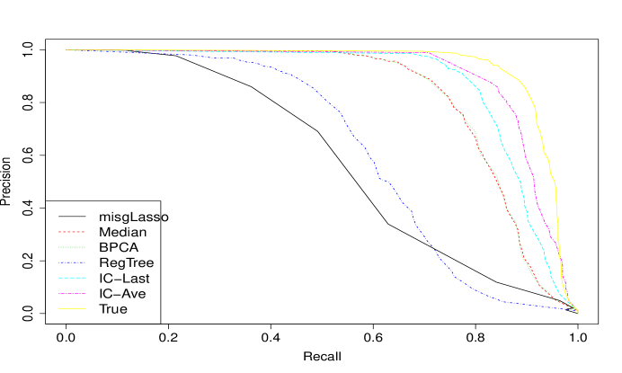
Figure 1: Precision-recall curves resulted from different imputation methods for one simulated dataset with $p=400$: “True” refers to the curve obtained with complete data; “misgLasso” refers to the curve produced by the misgLasso algorithm; “IC-Ave” and “IC-Last” refer to the curves obtained with the $\psi$-scores generated in the last IC iteration and averaged over last 20 IC iterations, respectively; and “Median”, “BPCA” and “RegTree” refer to the curves obtained with missing values imputed by the median filling, BPCA and regression tree methods, respectively.

For each dataset, the IC algorithm was run for 50 iterations. Figure 1 shows the resulting precision-recall curves for one dataset with $p=400$. For comparison, Figure 1 also includes the precision-recall curves produced by misgLasso and those produced by the $\psi$-learning algorithm with missing values imputed by the median filling, BPCA(Oba et al., 2003), and regression tree (Buuren and Groothuis-Oudshoorn, 2011) methods. The regression tree method has been implemented in the R package MICE and was applied to this example under its default setting. The misgLasso algorithm is a combination of the gLasso and EM algorithms, which is to integrate out the missing data as in the EM algorithm (see e.g., Städler and Bühlmann, 2012) and then learn the GGM using the gLasso algorithm. The misgLasso algorithm has been implemented in the R package spaceExt (He, 2011). Refer to Figure 1 of the Supplementary Material for the curves with other values of $p$.

Table 1: Average areas (over 10 datasets) under the Precision-Recall curves resulted from different imputation methods, where the number in the parentheses denotes the standard deviation of the average.

p	misgLasso	Median	BPCA	RegTree	IC-Last	IC-Ave	True
100	0.678(0.006)	0.882(0.007)	0.874(0.006)	0.817(0.005)	0.877(0.007)	0.904(0.006)	0.949(0.006)
200	0.633(0.005)	0.856(0.004)	0.855(0.004)	0.442(0.004)	0.887(0.004)	0.902(0.003)	0.941(0.002)
300	0.599(0.004)	0.830(0.003)	0.833(0.003)	0.574(0.003)	0.869(0.003)	0.901(0.002)	0.936(0.002)
400	0.580(0.003)	0.824(0.003)	0.824(0.003)	0.620(0.003)	0.868(0.003)	0.900(0.002)	0.932(0.001)

Table 1 compares the averaged areas (over 10 datasets) under the precision-recall curves produced by different methods. The comparison indicates that IC-Ave outperforms all others for this example. It is interesting to note that although IC-Last is also based on one-time imputation, it is much better than the median filling, regression tree and BPCA methods. This suggests that for microarray data, the model-based imputation method is potentially more accurate than other one-time imputation methods. The misgLasso algorithm does not work well for this example. This inferiority is not due to the EM algorithm, but due to the gLasso algorithm which does not work well for the example. This is consistent with Liang et al. (2015), where it is shown that the $\psi$-learning algorithm works much better than gLasso for the complete data version of this example.

3.3 Yeast Cell Expression Data

Gasch et al. (2000) explored genomic expression patterns in the yeast Saccharomyces cerevisiae responding to diverse environmental changes. The whole dataset has a missing rate of 3.01% and is available at http://genome-www.stanford.edu/yeast-stress/. Our numerical results for a subset of 1000 genes, reported in the Supplementary Material, indicate that the IC algorithm works reasonably well for this example with a few hub genes successfully identified, which are expected to play an important role for yeast cells in response to environmental changes.

4 High-Dimensional Variable Selection in Presence of Missing Data

This problem is also motivated by microarray data analysis, but the goal has been shifted to selection of genes relevant to a particular phenotype. To be more general, we let ${\bm{Y}}=(Y_{1},\ldots,Y_{n})^{T}$ denote the response vector for $n$ observations, and let ${\bm{X}}=(X_{1},\ldots,X_{n})^{T}$ denote the matrix of covariates, where each $X_{i}$ is a $p$-dimensional vector and $p$ can be much larger than $n$ (a.k.a. small-$n$-large-$p$). The response variable and covariates are linked through the regression,

$${\bm{Y}}=(\bm{1}_{n},{\bm{X}}){\bm{\beta}}+{\bm{\epsilon}},$$ (6)

where ${\bm{\beta}}=(\beta_{0},\beta_{1},\ldots,\beta_{p})^{T}$ denotes the vector of regression coefficients, and ${\bm{\epsilon}}\sim N(0,\sigma_{\epsilon}^{2}I_{n})$ denotes the vector of random errors.

Variable selection for the model (6) with complete data has been extensively studied in the recent literature. Methods have been developed from both frequentist and Bayesian perspectives, see e.g., Tibshirani (1996), Johnson and Rossell (2012), and Song and Liang (2015a). For incomplete data, Garcia et al. (2010) proposed to conduct variable selection by maximizing the penalized likelihood function of the incomplete data. However, when $p$ is large and the covariates $X_{i}$’s are generally correlated, the incomplete data likelihood function can be intractable, rendering failure of their method. Zhao and Long (2013) showed through numerical studies that for the high dimensional data the standard multiple imputation approach performs poorly, while the imputation method based on Bayesian Lasso often works better. However, since Bayesian Lasso tends to over-shrink the non-zero regression coefficients, its consistency in variable selection is hard to be justified when $p$ is much greater than $n$ (Castillo et al., 2015). Quite recently, Long and Johnson (2015) proposed to combine Bayesian Lasso imputation and stability selection (Meinshausen and Bühlmann, 2010). Again, the consistency of this method is hard to be justified due to the inconsistency of Bayesian Lasso.

4.1 The ICC Algorithm

In what follows, we consider a general setting of the model (6), where the covariates follow a multivariate Gaussian distribution ${\bm{X}}\sim N({\bm{\mu}},{\bm{\Sigma}})$. Under this setting, the parameter vector ${\bm{\theta}}$ consists of three natural blocks ${\bm{\beta}}$, $\sigma_{\epsilon}^{2}$ and the concentration matrix ${\bm{C}}={\bm{\Sigma}}^{-1}$. Since $n$ has been assumed to be smaller than $p$, we further assume the sparsity for both the regression coefficients ${\bm{\beta}}$ and the concentration matrix ${\bm{C}}$.

To apply the ICC algorithm to this problem, we choose the SIS-MCP algorithm as the consistent estimator of ${\bm{\beta}}$. That is, the variables are first subject to a sure independence screening procedure, and then the survived variables are selected using the MCP method (Zhang, 2010). This algorithm has been implemented in the R-package SIS. Given an estimates of ${\bm{\beta}}$, $\sigma_{\epsilon}^{2}$ can be estimated by $\hat{\sigma}_{\epsilon}^{2}=\sum_{i=1}^{n}\hat{\epsilon}_{i}^{2}/(n-|\hat{{\bm{\beta}}}|-1)$, where $\hat{\epsilon}_{i}$ denotes the residual of sample $i$, and $|\hat{{\bm{\beta}}}|$ denotes the number of nonzero elements included in the estimate $\hat{{\bm{\beta}}}$. Given the consistency of $\hat{{\bm{\beta}}}$, the consistency of $\hat{\sigma}_{\epsilon}^{2}$ is easy to be justified. To estimate the concentration matrix ${\bm{C}}$, we choose the $\psi$-learning algorithm. As mentioned previously, the $\psi$-learning algorithm provides a consistent estimate for the Gaussian graphical network, based on which a consistent estimate of the concentration matrix can be uniquely determined by the algorithm given in Hastie et al. (2009, p.634). Note that SIS-MCP does not make use of the dependency among the covariates. Given the structure of the ICC algorithm, some other variable selection algorithms which have made use of the dependency among the covariates, e.g., Yu and Liu (2016), can also be applied here.

Next, we consider the imputation step. Suppose that the value of $x_{hk}$ is missed in ${\bm{X}}$. Section 4 of the Supplementary Material presents the conditional distributions of $X_{hk}$ given ${\bm{Y}}$ and the rest elements of ${\bm{X}}$ under different scenarios. Based on the conditional distributions, $x_{hk}$ can be easily imputed by sampling from the respective samplized conditional distributions. Here the samplized conditional distribution refers to the distribution with its population parameters replaced by their respective estimates calculated from samples. For example, $\beta_{i}$’s are replaced by their SIS-MCP estimates, $\sigma_{\epsilon}^{2}$ is replaced by $\hat{\sigma}_{\epsilon}^{2}$, etc. In summary, the ICC algorithm works as follows:

• (Initialization) Fill each missing entry of ${\bm{X}}$ by the median of the corresponding variable, and then iterates between the CC- and I-steps.

• (CC-step) (i) Apply the SIS-MCP algorithm to estimate the regression coefficients ${\bm{\beta}}$; (ii) estimate $\sigma_{\epsilon}^{2}$ conditional on the estimate of ${\bm{\beta}}$; and (iii) apply the $\psi$-learning algorithm to learn the structure of the Gaussian graphical network.

• (I-step) Impute missing values according to the conditional distributions (given in the Supplemental Material) based on the regression model and network structure learned in the CC-step.

4.2 A Simulated Example

The datasets were simulated from the model (6) with $n=100$ and $p$=200 and 500. The covariates ${\bm{X}}$ were generated under two settings: (i) the covariates are mutually independent, where ${\bm{x}}_{i}\sim N(0,2I_{n})$ for $i=1,\ldots,n$; and (ii) the covariates are generated according to the concentration matrix (5). For both settings, we set $(\beta_{0},\beta_{1},\ldots,\beta_{5})=(1,1,2,-1.5,-2.5,5)$ and $\beta_{6}=\cdots=\beta_{p}=0$, and random error ${\bm{\epsilon}}\sim N(0,I_{n})$. For each pair of $(n,p)$, we simulated 10 datasets independently. For each dataset, we considered two missing rates, randomly deleting 5% and 10% entries of ${\bm{X}}$ as missing values. The performance of different methods was measured using three criteria:

$$\mbox{err}_{{\bm{\beta}}}^{2}=\|\hat{{\bm{\beta}}}-{\bm{\beta}}\|^{2},\quad\mbox{fsr}=\frac{|{\bm{s}}\backslash{\bm{s}}^{*}|}{|{\bm{s}}|},\quad\mbox{nsr}=\frac{|{\bm{s}}^{*}\backslash{\bm{s}}|}{|{\bm{s}}^{*}|},$$

where $\|\cdot\|$ denotes the Euclidean norm, $\hat{{\bm{\beta}}}$ denotes the estimate of ${\bm{\beta}}$, ${\bm{s}}^{*}$ denotes the set of true covariates, and ${\bm{s}}$ denotes the set of selected covariates.

The ICC algorithm was first applied to this example with the results summarized in Table 2 and 3. For each dataset, the algorithm was run for 30 iterations. For variable selection, we kept only the variables appeared 5 or more times in the last 10 iterations. For estimation of ${\bm{\beta}}$, we averaged the estimates of ${\bm{\beta}}$ obtained in the last 10 iterations. For comparison, we also tried the one-time imputation methods, including median filling and BPCA. As explained previously, the median filling method is to fill each missing value by the median of the corresponding variable, and BPCA is to impute the missing values based on the principal component regression. Then the variables are selected using the SIS-MCP method.

Table 2: Comparison of the ICC algorithm with the median filling and BPCA methods for high-dimensional variable selection with independent covariates. ”True” denotes the results obtained by the MCP method from the complete data. The values in the table are obtained by averaging over 10 independent datasets with the standard deviation reported in the parentheses.

$p$	Missing Rate		BPCA	Median	ICC	True
$200$		$\mbox{err}_{{\bm{\beta}}}^{2}$	0.257(0.267)	0.262(0.261)	0.042(0.041)	0.046(0.048)
	5%	fsr	0.119(0.143)	0.082(0.092)	0(0)	0(0)
		nsr	0(0)	0(0)	0(0)	0(0)
		$\mbox{err}_{{\bm{\beta}}}^{2}$	0.903(0.396)	0.856(0.421)	0.065(0.087)	0.046(0.048)
	10%	fsr	0.310(0.159)	0.308(0.178)	0(0)	0(0)
		nsr	0(0)	0(0)	0(0)	0(0)
$500$		$\mbox{err}_{{\bm{\beta}}}^{2}$	0.339(0.214)	0.350(0.206)	0.029(0.034)	0.027(0.023)
	5%	fsr	0.249(0.225)	0.266(0.237)	0(0)	0(0)
		nsr	0(0)	0(0)	0(0)	0(0)
		$\mbox{err}_{{\bm{\beta}}}^{2}$	1.532(1.071)	1.354(0.895)	0.044(0.022)	0.027(0.023)
	10%	fsr	0.470(0.265)	0.420(0.255)	0(0)	0(0)
		nsr	0.033(0.070)	0.017(0.053)	0(0)	0(0)

Table 3: Comparison of the ICC algorithm with the median filling and BPCA methods for high-dimensional variable selection with dependent covariates. ”True” denotes the results obtained by the MCP method from the complete data.

$p$	Missing Rate		BPCA	Median	ICC	True
$200$		$\mbox{err}_{{\bm{\beta}}}^{2}$	0.580(0.413)	0.548(0.140)	0.118(0.097)	0.071(0.050)
	5%	fsr	0.262(0.204)	0.263(0.200)	0(0)	0(0)
		nsr	0.017(0.052)	0.017(0.052)	0(0)	0(0)
		$\mbox{err}_{{\bm{\beta}}}^{2}$	1.604(0.666)	1.575(0.974)	0.424(0.461)	0.071(0.050)
	10%	fsr	0.247(0.229)	0.273(0.238)	0(0)	0(0)
		nsr	0.100(0.086)	0.083(0.088)	0.033(0.070)	0(0)
$500$		$\mbox{err}_{{\bm{\beta}}}^{2}$	0.669(0.366)	0.717(0.358)	0.172(0.195)	0.096(0.083)
	5%	fsr	0.262(0.202)	0.289(0.236)	0(0)	0(0)
		nsr	0.017(0.053)	0.017(0.053)	0(0)	0(0)
		$\mbox{err}_{{\bm{\beta}}}^{2}$	2.752(2.306)	2.896(2.601)	0.578(0.587)	0.096(0.083)
	10%	fsr	0.297(0.230)	0.327(0.224)	0(0)	0(0)
		nsr	0.133(0.070)	0.133(0.070)	0.050(0.081)	0(0)

The comparison indicates that the ICC algorithm works extremely well for this example. For the case of independent covariates, its results are almost as good as those obtained from the complete data. In both cases, the ICC algorithm significantly outperforms the one-time imputation methods.

4.3 A Real Data Example

We analyzed one real gene expression dataset about Bardet-Biedl syndrome (Scheetz et al., 2006). The complete dataset contains 120 samples, where the expression level of the gene TRIM32 works as the response variable and the expression levels of 200 other genes work as the predictors. The dataset is available in the R package flare. We generated ten incomplete datasets from the complete one by randomly deleting 5% observations. For each incomplete dataset, we ran the ICC algorithm for 30 iterations and averaged the estimates of ${\bm{\beta}}$ obtained in the last 10 iterations as the final estimate. For comparison, the median filling and BPCA methods were also applied to this example. Table 4 summarizes the estimation errors of $\hat{{\bm{\beta}}}$ (with respect to ${\bm{\beta}}_{c}$, the estimate of ${\bm{\beta}}$ from the complete data) produced by the three methods for ten incomplete datasets.

Table 4: Estimation errors of $\hat{{\bm{\beta}}}$ (with respect to ${\bm{\beta}}_{c}$) produced by ICC, median filling and BPCA for the Bardet-Biedl syndrome example, where err${}_{{\bm{\beta}}}^{2}$ is calculated by averaging $\|\hat{{\bm{\beta}}}-{\bm{\beta}}_{c}\|^{2}$ over ten incomplete datasets, and “s.d.” represents the standard deviation of err${}_{{\bm{\beta}}}^{2}$.

Method	BPCA	Median	ICC
err${}_{{\bm{\beta}}}^{2}$	0.428	0.397	0.187
s.d.	0.091	0.086	0.040

We have also explored the results of variable selection. The complete data model selects 5 variables: v.153, v.180, v.185, v.87 and v.200. For the ICC, median filling and BPCA models, we count the selection frequency of each variable for the ten incomplete datasets. For the ICC models, the top 5 variables in selection frequency are v.153, v.185, v.180, v.87 and v.200, which are the same (ignoring the order) as the complete data model. For the median filling models, the top 5 variables are v.153, v.185, v.62, v.200 and v.54. For the BPCA models, the top 5 variables are v.153, v.87, v.185, v.62 and v.200. Both the results of ${\bm{\beta}}$ estimation and variable selection indicate the superiority of the ICC algorithm over the one-time imputation methods.

5 A Random Coefficient Linear Model

To further illustrate the use of the ICC algorithm, we consider a random coefficient linear model. Such a model often arises, for instance, in recommendation systems where the customers rate different items, e.g., products or service. Specifically, we simulate the data from the following model

$$\begin{split}&y_{ij}={\bm{x}}_{ij}^{T}{\bm{\beta}}+{\bm{z}}_{i}^{T}{\bm{\lambda}}_{i}+{\bm{w}}_{j}^{T}{\bm{\gamma}}_{j}+e_{ij},\\ &e_{ij}\sim N(0,\sigma^{2}),\quad{\bm{\lambda}}_{i}\sim N(0,\Lambda),\quad{\bm{\gamma}}_{j}\sim N(0,\Gamma),\\ \end{split}$$ (7)

where $y_{ij}$ represents the response for customer $i$ on item $j$. Assuming that there are $I$ customers and each customer responds to $J$ items. Thus, the dataset consists of a total of $n=IJ$ observations. The vector ${\bm{x}}_{ij}$ represents the covariates that characterize the customers and items, e.g., how and how long the customer has purchased the item; ${\bm{z}}_{i}$ represents customer-specific covariates such as gender, education and demographics; and ${\bm{w}}_{j}$ represents item-specific covariates, e.g., the manufacturer and category of the item. The vector ${\bm{\lambda}}_{i}$ represents the customer-specific (random) coefficients and ${\bm{\gamma}}_{j}$ represents the item-specific (random) coefficients. This model can be easily extended to the case where each customer responds to only a subset of items. For this model, we treat the random coefficients ${\bm{\lambda}}_{i}$’s and ${\bm{\gamma}}_{j}$’s as missing data, and are interested in estimation of ${\bm{\beta}}$. For simplicity, we assume that ${\bm{\beta}}$ is low-dimensional, although the whole dataset can be big when $I$ and/or $J$ become large. Under this assumption, the ICC algorithm is essentially reduced to the stochastic EM algorithm for this example. Instead of using the ICC algorithm in this straightforward way, we propose to use it under the Bayesian framework. This extends the applications of the ICC algorithm to Bayesian computation.

To conduct Bayesian analysis for the model, we assume the following semiconjugate priors:

$${\bm{\beta}}\sim N({\bm{\mu}}_{{\bm{\beta}}},\Sigma_{{\bm{\beta}}}),\quad\sigma^{2}\sim IG(a,b),\quad\Lambda\sim IW(\rho_{\Lambda},{\bm{R}}_{\Lambda}),\quad\Gamma\sim IW(\rho_{\Gamma},{\bm{R}}_{\Gamma}),$$ (8)

where $IG(\cdot,\cdot)$ denotes the inverted Gamma distribution, $IW(\cdot,\cdot)$ denotes the inverted Wishart distribution, and ${\bm{\mu}}_{{\bm{\beta}}}$, $\Sigma_{{\bm{\beta}}}$, $a$, $b$, $\rho_{\Lambda}$, ${\bm{R}}_{\Lambda}$, $\rho_{\Gamma}$, and ${\bm{R}}_{\Gamma}$ are hyperparameters to be specified by the user. Each of these priors is individually conjugate to the normal likelihood function, given the other parameters, although the joint prior is not conjugate. Given these priors, the full conditional posterior distributions are derived in Section 5 of the Supplementary Material. Since, under the low-dimensional setting, the mode of the full conditional posterior distribution provides a consistent estimator for the corresponding parameter, the ICC algorithm can work as follows:

• (Initialization) Initialize $\lambda_{i}$’s, $\gamma_{j}$’s, and all parameters by some random numbers.

• (CC-step) Estimate the parameters ${\bm{\beta}}$, $\Lambda$, $\Gamma$, and $\sigma^{2}$ by the mode of their respective full conditional posterior distributions.

• (I-step) Impute the values of ${\bm{\lambda}}_{i}$’s and ${\bm{\gamma}}_{j}$’s according to their respective full conditional posterior distributions.

Under the Bayesian framework, the ICC algorithm works in a similar way to the Gibbs sampler except that it replaces posterior samples of the parameters by their respective full conditional posterior modes. Also, in this case, it is reduced to a hybrid of data augmentation (Tanner & Wong, 1987) and iterative conditional modes (Besag, 1974) by using imputation for the missing data and conditional modes for the parameters. However, the ICC algorithm offers more, whose consistency step allows it to conduct parameter estimation based on sub-samples only and this can create great savings in computation for big data problems. For high-dimensional problems, if the choice of prior distributions ensures posterior consistency, then the above algorithm can still be employed.

Figure 3 of the supplementary material compares the sampling path and autocorrelations of the ICC and Gibbs samples. As expected, the comparison shows that the ICC algorithm can converge faster than the Gibbs sampler and, in addition, the samples generated by the ICC algorithm tend to have smaller variations than those by the Gibbs sampler. We are aware that the accuracy of the ICC estimates is achieved at the price that we scarify the variance information contained in the posterior samples. As pointed out by Nielsen (2000), the variance of the ICC samples reflects the information loss due to the missing data. However, for the random coefficient example, the variance information can be obtained from the full conditional posterior distributions (given in the Supplementary Material) by simply plugging the parameter estimates into their variances. This observation suggests a general strategy to improve simulations of the Gibbs sampler: At each iteration, we only need to draw samples for the components for which the posterior variance is not analytically available and also of interest to us, and the other components can be replaced by the mode of the respective full conditional posterior distributions. As aforementioned, the mode can be found with a subset of samples, which can be much cheaper than sampling from the full data conditional posterior. We expect that the proposed strategy can significantly facilitate Bayesian computation for big data problems. A further study of this proposed strategy will be reported elsewhere.

6 Discussion

In this paper, we have proposed the imputation-consistency algorithm, or the IC algorithm in short, as a general algorithm for dealing with high-dimensional missing data problems. Under quite general conditions, we show that the IC algorithm can lead to a consistent estimate for the parameters. We have also extended the IC algorithm to the case of multiple block parameters, which leads to the imputation-conditional consistency (ICC) algorithm. We illustrate the proposed algorithms using the high-dimensional Gaussian graphical models, high-dimensional variable selection, and a random coefficient model.

Like the EM algorithm for low-dimensional data, we expect that the IC/ICC algorithm can have many applications for high-dimensional data. With the IC/ICC algorithm, many problems can be much simplified, e.g., variable selection for high-dimensional mixture regression (Khalili and Chen, 2007) and variable selection for high-dimensional mixed effect models (Fan and Li, 2012). For the former, the group index of each sample can be treated as missing data, and then the IC algorithm can be applied: The I-step is to assign the samples into different groups and the C-step is to conduct variable selection for each group separately. For the latter, at each iteration of the IC algorithm, it is reduced to variable selection for a high-dimensional regression with fixed designs given imputed random effects.

To assess the convergence of IC simulations, we recommend the Gelman-Rubin statistic (Gelman and Rubin, 1992). Since the IC algorithm usually converges very fast, we do not recommend a long run. Our experience shows that 20 iterations have often been long enough to produce a stable parameter estimate. Due to the MCMC nature of IC simulations, we recommend the averaging method for parameter estimation, and allow a burn-in period before collecting the samples for averaging. In Section 3.2, we reported the results based on the last iteration is just to compare with other one-time imputation methods. Theoretically, the variation of the IC estimates collected at different iterations reflects the missing data information. Hence, in addition to the parameter estimates, one might report their variance over iterations. However, this information is often not of interest to us, we choose not to report them in the paper.

Please be aware that when a large amount of noise was brought into the system through missing data, the IC/ICC algorithm may fail to work as implied by condition (A3). Also, please be aware that the IC/ICC algorithm targets consistency by design. When the sample size is small, the consistent estimators might not be adequately accurate. Our numerical experience shows that in this case, the IC/ICC algorithm might not significantly outperform one-time imputation methods, such as median filling and BPCA, as there is no much information to use for improving imputation during iterations. In general, when the sample size increases, the IC/ICC algorithm can significantly outperform one-time imputation methods.

Regarding statistical inference for parameters, we note that, theoretically, it can be done in general scenarios, not limited to that the posterior distribution of the parameters has a closed form. For example, for high-dimensional regression, if the Lasso algorithm is employed as the consistent estimator in the IC algorithm, then the inference for ${\bm{\theta}}$, e.g., constructing confidence intervals for each component of ${\bm{\theta}}$, can be done using the de-sparsified method (Zhang and Zhang, 2014; van de Geer et al., 2014). Let $V({\bm{x}}^{{\rm obs}},{\tilde{\bm{x}}}^{{\rm mis}}_{t},{\bm{\theta}}_{n}^{(t)})$ denote an uncertainty assessment statistic obtained at iteration $t$. Assume that $V({\bm{x}}^{{\rm obs}},{\bm{x}}^{{\rm mis}},{\bm{\theta}})$ is a Lipschitz function with respect to ${\bm{\theta}}$ and it is integrable. Then, by Corollary 3 or Corollary 4 (depending on IC or ICC being used), we will be able to get an uncertainty assessment for ${\bm{\theta}}$ by averaging $V({\bm{x}}^{{\rm obs}},{\tilde{\bm{x}}}^{{\rm mis}}_{t},{\bm{\theta}}_{n}^{(t)})$ along the IC/ICC chain. However, how to get the uncertainty assessment statistic $V({\bm{x}}^{{\rm obs}},{\tilde{\bm{x}}}^{{\rm mis}}_{t},{\bm{\theta}}_{n}^{(t)})$ for general high-dimensional problems is beyond the scope of this paper.

As a variant of the ICC algorithm, we note that the I-step can be replaced by an E-step if it is available. In this case, the C-step is to maximize the objective function

$$\max_{{\bm{\theta}}}E_{{\bm{\theta}}^{*}}Q({\bm{x}}^{{\rm obs}},{\bm{\theta}}|{\bm{\theta}}_{n}^{(t)}),$$ (9)

where the Q-function is as defined in the EM algorithm, and $E_{{\bm{\theta}}^{*}}$ denotes expectation with respect to the true distribution $\pi({\bm{x}}^{{\rm obs}}|{\bm{\theta}}^{*})$. Suppose that ${\bm{\theta}}$ has been partitioned into a few blocks ${\bm{\theta}}=(\theta^{(1)},\ldots,\theta^{(k)})$. To solve (9), the ICC algorithm is reduced to a blockwise consistency algorithm, which is to iteratively find consistent estimates for the parameters of each block conditioned on the current estimates of the parameters of other blocks. The blockwise consistency algorithm is closely related to, but more flexible than, the coordinate ascent algorithm (Tseng, 2001; Tseng and Yun, 2009). The coordinate ascent algorithm is to iteratively find the exact maximizer for each block conditioned on the current estimates of the parameters of other blocks. Under appropriate conditions, such as contraction as in (A5^′) and uniform consistency of ${\bm{\theta}}_{n}^{(t)}$’s as shown in Theorem 2, we will be able to show that the paths of the two algorithms will converge to the same point. This will be explored elsewhere.

The ICC algorithm have strong implications for big data computing. Based on the ICC algorithm, we have proposed a general strategy to improve Bayesian computation under big data scenario; that is, we can replace posterior samples by posterior modes in Gibbs iterations to accelerate simulations, where the posterior modes can be calculated with a subset of samples. In addition, the IC/ICC algorithm facilitates data integration from multiple sources when missing data are present. With the IC/ICC algorithm, the problem of data integration for incomplete data is converted to a problem for complete data and thus many of the existing meta-analysis methods can be conveniently applied for inference. This is very important for big data analysis.

Appendix

1. Proof of Consistency of ${\bm{\theta}}_{n}^{(t+1)}$.

Define $\Theta_{n}$ as the parameter space of ${\bm{\theta}}$, where the subscript $n$ indicates the dependence of the dimension of ${\bm{\theta}}$ on the sample size $n$. Without possible confusion, we will refer to $\Theta_{n}$ as $\Theta$. In addition, we let $\Theta_{n}^{T}=\{\theta_{n}^{(1)},\ldots,\theta_{n}^{(T)}\}$ denote a path of $\theta_{n}$ in the IC algorithm, which can be considered as an arbitrary subset of $\Theta_{n}$ with $T$ elements (replicates are allowed). Let $\tilde{x}=(x^{{\rm obs}},{\tilde{x}}^{{\rm mis}})$ and define

$$\begin{split}G_{n}({\bm{\theta}}|{\bm{\theta}}_{n}^{(t)})&=E_{{\bm{\theta}}_{n}^{(t)}}\log f_{{\bm{\theta}}}(\tilde{x})=\int\log(f_{{\bm{\theta}}}(\tilde{x}))f(x^{{\rm obs}}|{\bm{\theta}}^{*})h({\tilde{x}}^{{\rm mis}}|{\bm{\theta}}_{n}^{(t)})d\tilde{x},\\ \hat{G}_{n}({\bm{\theta}}|\tilde{\bm{x}},{\bm{\theta}}_{n}^{(t)})&=\frac{1}{n}\sum_{i=1}^{n}\log f(x^{{\rm obs}}_{i},{\tilde{x}}^{{\rm mis}}_{i}|{\bm{\theta}}),\\ \tilde{G}_{n}({\bm{\theta}}|{\bm{\theta}}_{n}^{(t)})&=\frac{1}{n}\sum_{i=1}^{n}\int\log f(x^{{\rm obs}}_{i},{\tilde{x}}^{{\rm mis}}|{\bm{\theta}})h({\tilde{x}}^{{\rm mis}}|x^{{\rm obs}}_{i},{\bm{\theta}}_{n}^{(t)})d{\tilde{x}}^{{\rm mis}}:=\frac{1}{n}\sum_{i=1}^{n}q(x^{{\rm obs}}_{i}).\end{split}$$ (10)

Our first goal is to show the following uniform law of large numbers (ULLN) holds for any $T$ such that $\log T=o(n)$:

$$\sup_{{\bm{\theta}}_{n}^{(t)}\in\Theta_{n}^{T}}\sup_{{\bm{\theta}}\in\Theta_{n}}|\hat{G}_{n}({\bm{\theta}}|\tilde{\bm{x}},{\bm{\theta}}_{n}^{(t)})-G_{n}({\bm{\theta}}|{\bm{\theta}}_{n}^{(t)})|\rightarrow_{p}0,$$ (11)

where $\rightarrow_{p}$ denotes convergence in probability. To achieve this goal, we need the following conditions:

• $\log f_{{\bm{\theta}}}(\tilde{x})$ is a continuous function of ${\bm{\theta}}$ for each $\tilde{x}\in\mathcal{X}$ and a measurable function of $\tilde{x}$ for each $\theta$.

• [Conditions for Glivenko-Cantelli theorem]

  • There exists a function $m_{n}(\tilde{x})$ such that $\sup_{{\bm{\theta}}\in\Theta_{n},\tilde{x}\in\mathcal{X}}|\log f_{{\bm{\theta}}}(\tilde{x})|\leq m_{n}(\tilde{x})$.

  • Define $\tilde{m}_{n}(x^{{\rm obs}},{\bm{\theta}}_{n}^{(t)})=\int m_{n}(\tilde{x})$ $h({\tilde{x}}^{{\rm mis}}|x^{{\rm obs}},{\bm{\theta}}_{n}^{(t)})d{\tilde{x}}^{{\rm mis}}$. Assume that there exists $m^{*}_{n}(x^{{\rm obs}})$ such that $0\leq\tilde{m}_{n}(x^{{\rm obs}},{\bm{\theta}}_{n}^{(t)})\leq m^{*}_{n}(x^{{\rm obs}})$ for all ${\bm{\theta}}_{n}^{(t)}$, $E[m^{*}_{n}(x^{{\rm obs}})]$ $<\infty$, and $\sup_{n\in\mathbb{Z}^{+}}E[m_{n}^{*}(x^{{\rm obs}})$ $1(m_{n}^{*}(x^{{\rm obs}})\geq\zeta)]\rightarrow 0$ as $\zeta\rightarrow\infty$. In addition, $\sup_{n\geq 1}\sup_{x\in\mathcal{X},{\bm{\theta}}\in\Theta_{n}}$ $|\int m_{n}(\tilde{x})1(m_{n}(\tilde{x})>\zeta)h({\tilde{x}}^{{\rm mis}}|x,{\bm{\theta}})d{\tilde{x}}^{{\rm mis}}|\rightarrow 0$ as $\zeta\rightarrow\infty$.

  • Define $\mathcal{F}_{n}=\{\int\log f(x^{{\rm obs}},{\tilde{x}}^{{\rm mis}}|{\bm{\theta}})h({\tilde{x}}^{{\rm mis}}|x^{{\rm obs}}$, ${\bm{\theta}}_{n}^{(t)})d{\tilde{x}}^{{\rm mis}}|{\bm{\theta}},{\bm{\theta}}_{n}^{(t)}\in\Theta_{n}\}$, and $\mathcal{G}_{n,M}=\{q1(m^{*}_{n}(x^{{\rm obs}})$ $\leq M)|q\in\mathcal{F}_{n}\}$. Suppose that for every $\epsilon$ and $M>0$, the metric entropy $\log N(\epsilon,\mathcal{G}_{n,M},L_{1}(\mathbb{P}_{n}))=o_{p}^{*}(n)$, where $\mathbb{P}_{n}$ is the empirical measure of $x^{{\rm obs}}$, and $N(\epsilon,\mathcal{G}_{n,M},L_{1}(\mathbb{P}_{n}))$ is the covering number with respect to the $L_{1}(\mathbb{P})$-norm.

• [Conditions for imputed data] Define $Z_{t,i}=\log f(x^{{\rm obs}}_{i},{\tilde{x}}^{{\rm mis}}_{i}|{\bm{\theta}})-\int\log f(x^{{\rm obs}}_{i},{\tilde{x}}^{{\rm mis}}|{\bm{\theta}})h({\tilde{x}}^{{\rm mis}}|$ $x^{{\rm obs}}_{i},{\bm{\theta}}_{n}^{(t)})$ $d{\tilde{x}}^{{\rm mis}}$. Suppose that for any ${\bm{\theta}}$ and ${\bm{\theta}}_{n}^{(t)}\in\Theta_{n}$, $E|Z_{t,i}|^{m}\leq m!M_{b}^{m-2}v_{i}/2$ for every $m\geq 2$ and some constants $M_{b}>0$ and $v_{i}=O(1)$. That is, $Z_{t,i}$’s are sub-exponential random variables.

Theorem 1.

Assume conditions (A1)–(A3), then (11) holds for any $T$ such that $\log T=o(n)$.

Proof.

By the definitions in (10), we have the decomposition

$$\hat{G}_{n}({\bm{\theta}}|\tilde{\bm{x}},{\bm{\theta}}_{n}^{(t)})-G_{n}({\bm{\theta}}|{\bm{\theta}}_{n}^{(t)})=\big{\{}\hat{G}_{n}({\bm{\theta}}|\tilde{\bm{x}},{\bm{\theta}}_{n}^{(t)})-\tilde{G}_{n}({\bm{\theta}}|{\bm{\theta}}_{n}^{(t)})\big{\}}+\big{\{}\tilde{G}_{n}({\bm{\theta}}|{\bm{\theta}}_{n}^{(t)})-G_{n}({\bm{\theta}}|{\bm{\theta}}_{n}^{(t)})\big{\}},$$ (12)

which consists of two terms, the first term comes from imputation of missing data, and the second term comes from the observed data.

First, we show that the second term of (12) converges to 0 uniformly, following the proof of Theorem 2.4.3 of van der Vaart and Wellner (1996). By the symmetrization Lemma 2.3.1 of van der Vaart and Wellner (1996), measurability of the class $\mathcal{F}_{n}$, and Fubini’s theorem,

$$\begin{split}&E^{*}\sup_{{\bm{\theta}},{\bm{\theta}}_{n}^{(t)}\in\Theta_{n}}|\tilde{G}_{n}({\bm{\theta}}|{\bm{\theta}}_{n}^{(t)})-G_{n}({\bm{\theta}}|{\bm{\theta}}_{n}^{(t)})|\leq 2E_{x^{{\rm obs}}}E_{\epsilon}\sup_{q(x)\in\mathcal{F}_{n}}\|\frac{1}{n}\sum_{i=1}^{n}\epsilon_{i}q(x_{i}^{obs})\|\\ &\leq 2E_{x^{{\rm obs}}}E_{\epsilon}\sup_{q(x)\in\mathcal{G}_{n,M}}\|\frac{1}{n}\sum_{i=1}^{n}\epsilon_{i}q(x_{i}^{obs})\|+2E^{*}[m^{*}_{n}(x^{obs})1(m^{*}_{n}(x^{obs})>M)],\\ \end{split}$$

where $\epsilon_{i}$ are i.i.d. Rademacher random variables with $P(\epsilon_{i}=+1)=P(\epsilon_{i}=-1)=1/2$, and $E^{*}$ denotes the outer expectation.

By condition (A2), $2E^{*}[m^{*}_{n}(x^{{\rm obs}})1(m^{*}_{n}(x^{{\rm obs}})>M)]\rightarrow 0$ for sufficiently large $M$. To prove convergence in mean, it suffices to show that the first term converges to zero for fixed $M$. Fix $x^{{\rm obs}}_{1},...,x^{{\rm obs}}_{n}$, and let $\mathcal{H}$ be a $\epsilon$-net in $L_{1}(\mathbb{P}_{n})$ over $\mathcal{G}_{n,M}$, then

$$E_{\epsilon}\sup_{q(x)\in\mathcal{G}_{n,M}}\|\frac{1}{n}\sum_{i=1}^{n}\epsilon_{i}q(x^{{\rm obs}}_{i})\|\leq E_{\epsilon}\sup_{q(x)\in\mathcal{H}}\|\frac{1}{n}\sum_{i=1}^{n}\epsilon_{i}q(x^{{\rm obs}}_{i})\|+\epsilon.$$

The cardinality of $\mathcal{H}$ can be chosen equal to $N(\epsilon,\mathcal{G}_{n,M},L_{1}(\mathbb{P}_{n})$. Bound the $L_{1}$-norm on the right by the Orlicz-norm $\psi_{2}$ and use the maximal inequality (Lemma 2.2.2 of van der Vaart and Wellner (1996)) and Hoeffding’s inequality, it can be shown that

$$E_{\epsilon}\sup_{q(x)\in\mathcal{G}_{n,M}}\|\frac{1}{n}\sum_{i=1}^{n}\epsilon_{i}q(x^{{\rm obs}}_{i})\|\leq K\sqrt{1+\log N(\epsilon,\mathcal{G}_{n,M},L_{1}(\mathbb{P}_{n}))}\sqrt{6/n}M+\epsilon\rightarrow_{P^{*}}\epsilon,$$ (13)

where $K$ is a constant, and $P^{*}$ denotes outer probability. It has been shown that the left side of (13) converges to zero in probability. Since it is bounded by $M$, its expectation with respect to $x^{{\rm obs}}_{1},\ldots,x^{{\rm obs}}_{n}$ converges to zero by the dominated convergence theorem.

This concludes the proof that $\sup_{{\bm{\theta}}_{n}^{(t)}\in\Theta_{n}}\sup_{{\bm{\theta}}\in\Theta_{n}}|\tilde{G}_{n}({\bm{\theta}}|{\bm{\theta}}_{n}^{(t)})-G_{n}({\bm{\theta}}|{\bm{\theta}}_{n}^{(t)})|\rightarrow_{p}0$ in mean. Further, by Markov inequality, we conclude that

$$\sup_{{\bm{\theta}}_{n}^{(t)}\in\Theta_{n}}\sup_{{\bm{\theta}}\in\Theta_{n}}|\tilde{G}_{n}({\bm{\theta}}|{\bm{\theta}}_{n}^{(t)})-G_{n}({\bm{\theta}}|{\bm{\theta}}_{n}^{(t)})|\to_{p}0.$$ (14)

To establish the uniform convergence of the first term of (12), we fix $x^{{\rm obs}}_{1},...,x^{{\rm obs}}_{n}$. By condition (A3), $n(\hat{G}_{n}({\bm{\theta}}|\tilde{x},{\bm{\theta}}_{n}^{(t)})-\tilde{G}_{n}({\bm{\theta}}|{\bm{\theta}}_{n}^{(t)}))=Z_{t,1}+Z_{t,2}+\cdots+Z_{t,n}$. By Bernstein’s inequality,

$$P(n|\hat{G}_{n}({\bm{\theta}}|\tilde{x},{\bm{\theta}}_{n}^{(t)})-\tilde{G}_{n}({\bm{\theta}}|{\bm{\theta}}_{n}^{(t)})|>z)=P(|Z_{t,1}+Z_{t,2}+\cdots+Z_{t,n}|>z)\leq 2\exp\left\{-\frac{1}{2}\frac{z^{2}}{v+M_{b}z}\right\},$$

for $v\geq v_{1}+\cdots+v_{n}$. By Lemma 2.2.10 of van der Vaart and Wellner (1996), for Orlicz norm $\psi_{1}$, we have

$$\begin{split}&\|\sup_{{\bm{\theta}}\in\Theta_{n},t=1,2,\ldots,T}n\big{\{}\hat{G}_{n}({\bm{\theta}}|\tilde{\bm{x}},{\bm{\theta}}_{n}^{(t)})-\tilde{G}_{n}({\bm{\theta}}|{\bm{\theta}}_{n}^{(t)})\big{\}}\|_{\psi_{1}}\\ &\leq\epsilon+K(M_{b}\log(1+TN(\epsilon,\mathcal{G}_{n,M},L_{1}(\mathbb{P}_{n})))+\sqrt{v}\sqrt{\log(1+TN(\epsilon,\mathcal{G}_{n,M},L_{1}(\mathbb{P}_{n})))}),\end{split}$$

for a constant $K$ and any $\epsilon>0$. By condition (A2)-(c) and the condition $\log(T)=o(n)$,

$$\begin{split}&\|\sup_{{\bm{\theta}}\in\Theta_{n},t=1,2,\ldots,T}\{\hat{G}_{n}({\bm{\theta}}|\tilde{\bm{x}},{\bm{\theta}}_{n}^{(t)})-\tilde{G}_{n}({\bm{\theta}}|{\bm{\theta}}_{n}^{(t)})\}\|_{\psi_{1}}\\ &\leq\epsilon+K(M_{b}\log(1+TN(\epsilon,\mathcal{G}_{n,M},L_{1}(\mathbb{P}_{n})))/n+\sqrt{v/n}\sqrt{\log(1+TN(\epsilon,\mathcal{G}_{n,M},L_{1}(\mathbb{P}_{n})))/n})\rightarrow_{P^{*}}\epsilon.\end{split}$$

Therefore,

$$\sup_{{\bm{\theta}}\in\Theta_{n},t=1,2,...,T}|\hat{G}_{n}({\bm{\theta}}|\widetilde{x},{\bm{\theta}}_{n}^{(t)})-\tilde{G}_{n}({\bm{\theta}}|{\bm{\theta}}_{n}^{(t)})|\rightarrow_{p}0.$$ (15)

The theorem can then be concluded by combining (14) and (15). ∎

Remark R1 (On the metric entropy condition) Assume that all elements in $\cup_{n\geq 1}\mathcal{F}_{n}$ are uniformly Lipschitz with respect to the $L_{1}$-norm. Then the metric entropy $\log N(\epsilon,\mathcal{G}_{n,M},L_{1}(\mathbb{P}_{n}))$ can be measured based on the parameter space $\Theta$. Since the functions in $\mathcal{G}_{n,M}$ are all bounded, the corresponding parameter space $\Theta_{n,M}$ can be contained in a $L_{1}$-ball by the continuity of $\log f(\tilde{x}|{\bm{\theta}})$ in ${\bm{\theta}}$. Further, we assume that the diameter of the $L_{1}$-ball or the space $\Theta_{n,M}$ grows at a rate of $O(n^{\alpha})$ for some $0\leq\alpha<1/2$, then $\log N(\epsilon,\mathcal{G}_{n,M},L_{1}(\mathbb{P}_{n}))=O(n^{2\alpha}\log p)$ holds, which allows $p$ to grow at a polynomial rate of $O(n^{\gamma})$ for some constant $0<\gamma<\infty$. Note that the increased diameter accounts for the conventional assumption that the size of the true model grows with the sample size $n$. Refer to Vershynin (2015) for more discussions on this issue. Similar conditions on metric entropy have been used in the literature of high-dimensional statistics. For example, Raskutti et al. (2011) studied minimax rates of estimation for high-dimensional linear regression over $L_{q}$-balls.

Remark R2 (On the condition of $T$). Since the imputation step draws random data at each iteration $t$, there is no way to show uniform convergence of ${\bm{\theta}}_{n}^{(t+1)}$ to ${\bm{\theta}}_{*}^{(t)}$ over all possible ${\bm{\theta}}_{n}^{(t)}\in\Theta_{n}$. However, we are able to prove that the consistency results hold for any sequence of ${\bm{\theta}}_{n}^{(1)},...,{\bm{\theta}}_{n}^{(T)}$ with $T$ being not too large compared to $e^{n}$. This is enough for Theorems 3-6. To justify this, we may consider the case that the dimension of ${\bm{\theta}}_{n}$ grows with $n$ at a rate of $p=O(n^{\gamma})$ for a constant $\gamma>0$, say, $\gamma=5$. Then it is easy to see that when $n>13$, the ratio $T/p$ has an order of

$$O(e^{n}/p)=O(e^{n-\gamma\log(n)})\succ O(e^{0.1n})\succ O(p^{100}),$$

which implies that essentially there is no constraint on the setting of $T$. Note that for MCMC simulations, the number of iterations is often set to a low-order polynomial of $p$ for a given set of observations.

For any ${\bm{\theta}}_{n}^{(t)}\in\Theta_{n}^{T}$, we define ${{\bm{\theta}}}_{n}^{(t+1)}=\arg\max_{{\bm{\theta}}\in\Theta_{n}}\hat{G}_{n}({\bm{\theta}}|\widetilde{x},{\bm{\theta}}_{n}^{(t)})$ and ${\bm{\theta}}_{*}^{(t)}=\arg\max_{{\bm{\theta}}\in\Theta_{n}}G_{n}({\bm{\theta}}|{\bm{\theta}}_{n}^{(t)})$. We would like to establish the uniform consistency of ${{\bm{\theta}}}_{n}^{(t+1)}$ with respect to $t$, i.e.,

$$\sup_{t\in\{1,2,\ldots,T\}}\|{{\bm{\theta}}}_{n}^{(t+1)}-{\bm{\theta}}_{*}^{(t)}\|\to_{p}0,\quad\mbox{as $n\to\infty$}.$$ (16)

To achieve this goal, we assume the following condition:

• For each $t=1,2,\ldots,T$, $G_{n}({\bm{\theta}}|{\bm{\theta}}_{n}^{(t)})$ has a unique maximum at ${\bm{\theta}}_{*}^{(t)}$; for any $\epsilon>0$, $\sup_{{\bm{\theta}}\in\Theta_{n}\setminus B_{t}(\epsilon)}G_{n}({\bm{\theta}}|{\bm{\theta}}_{n}^{(t)})$ exists, where $B_{t}(\epsilon)=\{{\bm{\theta}}\in\Theta_{n}:\|{\bm{\theta}}-{\bm{\theta}}_{*}^{(t)}\|<\epsilon\}$. Let $\delta_{t}=G_{n}({\bm{\theta}}_{*}^{(t)}|{\bm{\theta}}_{n}^{(t)})-\sup_{{\bm{\theta}}\in\Theta_{n}\setminus B_{t}(\epsilon)}G_{n}({\bm{\theta}}|{\bm{\theta}}_{n}^{(t)})$, $\delta=\min_{t\in\{1,2,\ldots,T\}}\delta_{t}>0$.

Note that the existence of $\sup_{{\bm{\theta}}\in\Theta_{n}\setminus B_{t}(\epsilon)}G_{n}({\bm{\theta}}|{\bm{\theta}}_{n}^{(t)})$ can be easily satisfied if $\Theta_{n}$ is restricted to a compact set, which implies that $\Theta_{n}\setminus B_{t}(\epsilon)$ is also a compact set and thus the supremum is achievable. This condition can also be satisfied by assuming that $\Theta_{n}$ is convex and for each $t$, ${\bm{\theta}}_{*}^{(t)}$ is in the interior of $\Theta_{n}$ and $G_{n}({\bm{\theta}}|{\bm{\theta}}_{n}^{(t)})$ is concave in ${\bm{\theta}}$.

Theorem 2.

Assume conditions (A1)-(A4) hold, then the maximum pseudo-complete data likelihood estimate ${{\bm{\theta}}}_{n}^{(t+1)}$ is uniformly consistent to ${\bm{\theta}}_{*}^{(t)}$ over $t=1,2,\ldots,T$, i.e. (16) holds.

Proof.

Since both $\hat{G}_{n}({\bm{\theta}}|\widetilde{x},{\bm{\theta}}_{n}^{(t)})$ and $G_{n}({\bm{\theta}}|{\bm{\theta}}_{n}^{(t)})$ are continuous in $\theta$ as implied by the continuity of $\log f_{{\bm{\theta}}}(\tilde{\bm{x}})$, the remaining part of the proof follows from Lemma 1 by setting the penalty function $P_{\lambda_{n}}({\bm{\theta}})=0$ for all ${\bm{\theta}}\in\Theta_{n}$. ∎

Lemma 1.

Consider a sequence of functions $Q_{t}({\bm{\theta}},{\bm{X}}_{n})$ for $t=1,2,\ldots,T$. Suppose that the following conditions are satisfied: (B1) For each $t$, $Q_{t}({\bm{\theta}},{\bm{X}}_{n})$ is continuous in ${\bm{\theta}}$ and there exists a function $Q_{t}^{*}({\bm{\theta}})$, which is continuous in ${\bm{\theta}}$ and uniquely maximized at ${\bm{\theta}}_{*}^{(t)}$. (B2) For any $\epsilon>0$, $\sup_{{\bm{\theta}}\in\Theta_{n}\setminus B_{t}(\epsilon)}Q_{t}^{*}({\bm{\theta}})$ exists, where $B_{t}(\epsilon)=\{{\bm{\theta}}:\|{\bm{\theta}}-{\bm{\theta}}_{*}^{(t)}\|<\epsilon\}$; Let $\delta_{t}=Q_{t}^{*}({\bm{\theta}}_{*}^{(t)})-\sup_{{\bm{\theta}}\in\Theta_{n}\setminus B_{t}(\epsilon)}Q_{t}^{*}({\bm{\theta}})$, $\delta=\min_{t\in\{1,2,\ldots,T\}}\delta_{t}>0$. (B3) $\sup_{t\in\{1,2,\ldots,T\}}\sup_{{\bm{\theta}}\in\Theta_{n}}|Q_{t}({\bm{\theta}},{\bm{X}}_{n})-Q_{t}^{*}({\bm{\theta}})|\to_{p}0$ as $n\to\infty$. (B4) The penalty function $P_{\lambda_{n}}({\bm{\theta}})$ is non-negative and converges to 0 uniformly over the set $\{{\bm{\theta}}_{*}^{(t)}:t=1,2,\ldots,T\}$ as $n\to\infty$, where $\lambda_{n}$ is a regularization parameter and its value can depend on the sample size $n$. Let ${\bm{\theta}}_{n}^{(t)}=\arg\max_{{\bm{\theta}}\in\Theta_{n}}\{Q_{t}({\bm{\theta}},{\bm{X}}_{n})-P_{\lambda_{n}}({\bm{\theta}})\}$. Then the uniform convergence holds, i.e., $\sup_{t\in\{1,2,\ldots,T\}}\|{\bm{\theta}}_{n}^{(t)}-{\bm{\theta}}_{*}^{(t)}\|\to_{p}0$.

Proof.

Consider two events (i) $\sup_{t\in\{1,2,\ldots,T\}}\sup_{{\bm{\theta}}\in\Theta_{n}\setminus B_{t}(\epsilon)}|Q_{t}({\bm{\theta}},{\bm{X}}_{n})-Q_{t}^{*}({\bm{\theta}})|<\delta/2$, and (ii) $\sup_{t\in\{1,2,\ldots,T\}}$ $\sup_{{\bm{\theta}}\in B_{t}(\epsilon)}|Q_{t}({\bm{\theta}},{\bm{X}}_{n})-Q_{t}^{*}({\bm{\theta}})|<\delta/2$. From event (i), we can deduce that for any $t\in\{1,2,\ldots,T\}$ and any ${\bm{\theta}}\in\Theta_{n}\setminus B_{t}(\epsilon)$, $Q_{t}({\bm{\theta}},{\bm{X}}_{n})<Q_{t}^{*}({\bm{\theta}})+\delta/2\leq Q_{t}^{*}({\bm{\theta}}_{*}^{(t)})-\delta_{t}+\delta/2\leq Q_{t}^{*}({\bm{\theta}}_{*}^{(t)})-\delta/2$. Therefore, $Q_{t}({\bm{\theta}},{\bm{X}}_{n})-P_{\lambda_{n}}({\bm{\theta}})<Q_{t}^{*}({\bm{\theta}}_{*}^{(t)})-\delta/2-o(1)$ by condition (B4).

From event (ii), we can deduce that for any $t\in\{1,2,\ldots,T\}$ and any ${\bm{\theta}}\in B_{t}(\epsilon)$, $Q_{t}({\bm{\theta}},{\bm{X}}_{n})>Q_{t}^{*}({\bm{\theta}})-\delta/2$ and $Q_{t}({\bm{\theta}}_{*}^{(t)},{\bm{X}}_{n})>Q_{t}^{*}({\bm{\theta}}_{*}^{(t)})-\delta/2$. Therefore, $Q_{t}({\bm{\theta}}_{*}^{(t)},{\bm{X}}_{n})-P_{\lambda_{n}}({\bm{\theta}}_{*}^{(t)})>Q_{t}^{*}({\bm{\theta}}_{*}^{(t)})-\delta/2-o(1)$ by condition (B4).

If both events hold simultaneously, then we must have ${{\bm{\theta}}}_{n}^{(t)}\in B_{t}(\epsilon)$ for all $t\in\{1,2,\ldots,T\}$ as $n\to\infty$. By condition (B3), the probability that both events hold tends to 1. Therefore,

$$P(\mbox{${\bm{\theta}}_{n}^{(t)}\in B_{t}(\epsilon)$ for all $t=1,2,\ldots,T$})\to 1,$$

which concludes the lemma. ∎

Theorem 2 establishes the consistency of ${{\bm{\theta}}}_{n}^{(t+1)}$ with respect to ${\bm{\theta}}_{*}^{(t)}$ for each $t=1,2,\ldots,T$. However, in the small-$n$-large-$p$ scenario, ${{\bm{\theta}}}_{n}^{(t+1)}$ is not well defined. For this reason, a sparsity constraint needs to be imposed on ${\bm{\theta}}$. For example, we can apply a regularization method to get an estimate of ${\bm{\theta}}_{*}^{(t)}$; that is, we can define

$${\bm{\theta}}_{n,p}^{(t+1)}=\arg\max_{{\bm{\theta}}\in\Theta_{n}}\left\{\hat{G}_{n}({\bm{\theta}}|\tilde{\bm{x}},{\bm{\theta}}_{n}^{(t)})-P_{\lambda_{n}}({\bm{\theta}})\right\},$$ (17)

where the penalty function $P_{\lambda_{n}}({\bm{\theta}})$ constrains the sparsity of the solution. Assume that

• The penalty function $P_{\lambda_{n}}({\bm{\theta}})$ is non-negative, ensures the existence of ${\bm{\theta}}_{n,p}^{(t+1)}$ for all $n\in\mathbb{N}$ and $t=1,2,\ldots,T$, and converges to 0 uniformly over the set $\{{\bm{\theta}}_{*}^{(t)}:t=1,2\ldots,T\}$ as $n\to\infty$.

Corollary 1.

If the conditions (A1)-(A4) and (C1) hold, then the regularization estimator ${\bm{\theta}}_{n,p}^{(t+1)}$ in (17) is uniformly consistent to ${\bm{\theta}}_{*}^{(t)}$ over $t=1,2,\ldots,T$, i.e., $\sup_{t\in\{1,2,\ldots,T\}}\|{\bm{\theta}}_{n,p}^{(t+1)}-{\bm{\theta}}_{*}^{(t)}\|\to_{p}0$ as $n\to\infty$.

Proof.

It follows the proof of Lemma 1 directly. ∎

Take the high-dimensional regression as example. If we allow $p$ to grow with $n$ at the rate $p=O(n^{\gamma})$ for some constant $\gamma>0$, allow the size of ${\bm{\beta}}_{*}^{(t)}$ for all $t$ to grow with $n$ at the rate $O(n^{\alpha})$ for some constant $0<\alpha<1/2$, choose $\lambda_{n}=O(\sqrt{\log(p)/n})$, and set $P_{\lambda_{n}}({\bm{\theta}})=\lambda_{n}\sum_{i=1}^{p}c_{\lambda_{n}}(|\theta_{i}|)$, where $c_{\lambda_{n}}(\cdot)$ is set in the form of SCAD (Fan and Li, 2001) or MCP (Zhang, 2010) penalties, then the condition (C1) is satisfied. For both the SCAD and MCP penalties, $c_{\lambda_{n}}(|\theta_{i}|)=0$ if $\theta_{i}=0$ and bounded by a constant otherwise. Similarly, if the beta-min assumption holds, i.e., there exists a constant $\beta_{\min}>0$ such that $\min_{j\in S^{*}}|\beta_{*j}|\geq\beta_{\min}$, where $S^{*}=\{j:\beta_{*j}\neq 0\}$ denotes the index set of non-zero regression coefficients, then the reciprocal Lasso penalty (Song and Liang, 2015b) also satisfies (C1). Note that, if $\Theta=\mathbb{R}^{p}$, the Lasso penalty does not satisfy (C1) as which is unbounded. This explains why the Lasso estimate is unbiased even as $n\to\infty$. However, if $\Theta_{n}$ is restricted to a bounded space, then the Lasso penalty also satisfies (C1).

Alternative to regularization methods, one may first restrict the space of ${\bm{\theta}}_{*}^{(t)}$ to some low-dimensional subspace through sure screening, and then find a consistent estimate in the subspace using a conventional statistical methods, such as maximum likelihood, moment estimation, or even regularization. Both the $\psi$-learning (Liang, Song and Qiu, 2015) sure independence screening (SIS) (Fan and Lv, 2008; Fan and Song, 2010) methods belong to this class. For $\psi$-learning, after correlation screening (based on the pseudo-complete data), the remaining network structure estimation procedure is essentially the same with the covariance selection method (Dempster, 1972) which, by nature, is a maximum likelihood estimation method. It is interesting to point out that the sure screening-based methods can be viewed as a special subclass of regularization methods, for which the solutions in the low-dimensional subspace receives a zero penalty, and those outside the subspace receives a penalty of $\infty$. It is easy to see that such a binary-type penalty function satisfies condition (C1).

Both the regularization and sure screening-based methods are constructive. In what follows, we give a proof for the use of general consistent estimation procedures in the IC algorithm. Let ${\bm{\theta}}_{n,g}^{(t+1)}$ denote the estimate of ${\bm{\theta}}_{*}^{(t)}$ produced by such a general consistent estimation procedure at iteration $t+1$. Corollary 2 shows that if ${\bm{\theta}}_{n,g}^{(t+1)}$ is accurate enough for each $t$ (pointwisely) and the log-likelihood function of the pseudo-complete data satisfies some moment conditions, then the estimation procedure can be used in the IC algorithm. Therefore, by its MLE nature in the subspace, the use of the $\psi$-learning algorithm in the IC algorithm can also be justified by Corollary 2.

• [Conditions for general consistent estimate ${\bm{\theta}}_{n,g}^{(t)}$] Assume that for each $t=1,2,\ldots,T$, ${\bm{\theta}}_{n,g}^{(t+1)}-{\bm{\theta}}_{*}^{(t)}=O_{p}(1/\sqrt{n})$ (pointwisely) and the Hessian matrix $\partial^{2}G_{n}({\bm{\theta}}|\tilde{\bm{x}},{\bm{\theta}}_{n}^{(t)})/\partial{\bm{\theta}}\partial{\bm{\theta}}^{\prime}$ is bounded in a neighborhood of ${\bm{\theta}}_{*}^{(t)}$; let

  $$Z_{t,i}^{\prime}=\log f(x^{{\rm obs}}_{i},{\tilde{x}}^{{\rm mis}}_{i}|{\bm{\theta}}_{n,g}^{(t+1)})-\int\log f(x^{{\rm obs}},{\tilde{x}}^{{\rm mis}}|{\bm{\theta}}_{n,g}^{(t+1)})f(x^{{\rm obs}}|{\bm{\theta}}^{*})h({\tilde{x}}^{{\rm mis}}|x^{{\rm obs}}_{i},{\bm{\theta}}_{n}^{(t)})d{\tilde{x}}^{{\rm mis}}dx^{{\rm obs}},$$

  then $E|Z_{t,i}^{\prime}|^{m}\leq m!\tilde{M}_{b}^{m-2}\tilde{v}_{i}/2$ for every $m\geq 2$ and some constants $\tilde{M}_{b}>0$ and $\tilde{v}_{i}=O(1)$.

Corollary 2.

Assume (A1)-(A4) and (C2). Then ${\bm{\theta}}_{n,g}^{(t+1)}$ is uniformly consistent to ${\bm{\theta}}_{*}^{(t)}$ over $t=1,2,\ldots,T$, i.e., $\sup_{t\in\{1,2,\ldots,T\}}\|{\bm{\theta}}_{n,g}^{(t+1)}-{\bm{\theta}}_{*}^{(t)}\|\to_{p}0$ as $n\to\infty$.

Proof.

Applying Taylor expansion to $G_{n}({\bm{\theta}}|{\bm{\theta}}_{n}^{(t)})$ at ${\bm{\theta}}_{*}^{(t)}$, we get $G_{n}({\bm{\theta}}_{n,g}^{(t+1)}|{\bm{\theta}}_{n}^{(t)})-G_{n}({\bm{\theta}}_{*}^{(t)}|{\bm{\theta}}_{n}^{(t)})=O_{p}(1/n)$, following from condition (C2) and condition (A4) that $G_{n}({\bm{\theta}}|{\bm{\theta}}_{n}^{(t)})$ is maximized at ${\bm{\theta}}_{*}^{(t)}$. Therefore,

$$\begin{split}n[\hat{G}_{n}({\bm{\theta}}_{n,g}^{(t+1)}|\tilde{\bm{x}},{\bm{\theta}}_{n}^{(t)})-G_{n}({\bm{\theta}}_{*}^{(t)}|{\bm{\theta}}_{n}^{(t)})]&=Z_{t,1}^{\prime}+\cdots+Z_{t,n}^{\prime}+n[G_{n}({\bm{\theta}}_{n,g}^{(t+1)}|{\bm{\theta}}_{n}^{(t)})-G_{n}({\bm{\theta}}_{*}^{(t)}|{\bm{\theta}}_{n}^{(t)})]\\ &=Z_{t,1}^{\prime}+\cdots+Z_{t,n}^{\prime}+\epsilon_{n},\\ \end{split}$$

where $\epsilon_{n}=O_{p}(1)$, and

$$P(n|\hat{G}_{n}({\bm{\theta}}_{n,g}^{(t+1)}|\tilde{\bm{x}},{\bm{\theta}}_{n}^{(t)})-G_{n}({\bm{\theta}}_{*}^{(t)}|{\bm{\theta}}_{n}^{(t)})|>nz)\leq P(|Z_{t,1}^{\prime}+\cdots+Z_{t,n}^{\prime}|>nz-|\epsilon_{n}|).$$ (18)

By Bernstein’s inequality,

$$P(|Z_{t,1}^{\prime}+\cdots+Z_{t,n}|>nz-|\epsilon_{n}|)\leq 2\exp\left\{-\frac{1}{2}\frac{(z-|\epsilon_{n}|/n)^{2}}{\tilde{v}^{\prime}+\tilde{M}_{b}^{\prime}(z-|\epsilon_{n}|/n)}\right\},$$ (19)

for $\tilde{v}^{\prime}\geq(\tilde{v}_{1}+\cdots+\tilde{v}_{n})/n^{2}$ and $\tilde{M}_{b}^{\prime}=\tilde{M}_{b}/n$. Applying Taylor expansion to the right of (19) at $z$ and combining with (18) leads to

$$P(|\hat{G}_{n}({\bm{\theta}}_{n,g}^{(t+1)}|\tilde{\bm{x}},{\bm{\theta}}_{n}^{(t)})-G_{n}({\bm{\theta}}_{*}^{(t)}|{\bm{\theta}}_{n}^{(t)})|>z)\leq K\exp\left\{-\frac{1}{2}\frac{z^{2}}{\tilde{v}^{\prime}+\tilde{M}_{b}^{\prime}z}\right\},$$ (20)

where $K=2+\frac{3}{\tilde{M}_{b}^{\prime}}O_{p}(1/n)=2+\frac{3}{\tilde{M}_{b}}O_{p}(1)$, since the derivative $|d[z^{2}/(\tilde{v}^{\prime}+\tilde{M}_{b}^{\prime}z)]/dz|\leq 3/\tilde{M}_{b}^{\prime}$.

As in the proof of Theorem 1, by applying Lemma 2.2.10 of van der Vaart and Wellner (1996), we can prove

$$\sup_{{\bm{\theta}}_{n}^{(t)}\in\Theta_{n},t\in\{1,2,\ldots,T\}}\left|\hat{G}_{n}({\bm{\theta}}_{n,g}^{(t+1)}|\tilde{\bm{x}},{\bm{\theta}}_{n}^{(t)})-G_{n}({\bm{\theta}}_{*}^{(t)}|{\bm{\theta}}_{n}^{(t)})\right|\to_{p}0.$$ (21)

Note that, as implied by the proof of Lemma 2.2.10 of van der Vaart and Wellner (1996), (21) holds for a general constant $K$ in (20). Then, by condition (A4), we must have the uniform convergence that ${\bm{\theta}}_{n,g}^{(t+1)}\in B_{t}(\epsilon)$ for all $t$ as $n\to\infty$, where $B_{t}(\epsilon)$ is as defined in (A4). This statement can be proved by contradiction as follows:

Assume ${\bm{\theta}}_{n,g}^{(i+1)}\notin B_{i}(\epsilon)$ for some $i\in\{1,2,\ldots,T\}$. By the uniform convergence established in Theorem 1, $\left|\hat{G}_{n}({\bm{\theta}}_{n,g}^{(i+1)}|\tilde{\bm{x}},{\bm{\theta}}_{n}^{(i)})-G_{n}({\bm{\theta}}_{n,g}^{(i+1)}|{\bm{\theta}}_{n}^{(i)})\right|=o_{p}(1)$. Further, by condition (A4) and the assumption ${\bm{\theta}}_{n,g}^{(i+1)}\notin B_{i}(\epsilon)$,

$$\begin{split}\left|\hat{G}_{n}({\bm{\theta}}_{n,g}^{(i+1)}|\tilde{\bm{x}},{\bm{\theta}}_{n}^{(i)})-G_{n}({\bm{\theta}}_{*}^{(i)}|{\bm{\theta}}_{n}^{(i)})\right|&\geq\left|G_{n}({\bm{\theta}}_{n,g}^{(i+1)}|{\bm{\theta}}_{n}^{(i)})-G_{n}({\bm{\theta}}_{*}^{(i)}|{\bm{\theta}}_{n}^{(i)})\right|-\left|\hat{G}_{n}({\bm{\theta}}_{n,g}^{(i+1)}|\tilde{\bm{x}},{\bm{\theta}}_{n}^{(i)})-G_{n}({\bm{\theta}}_{n,g}^{(i+1)}|{\bm{\theta}}_{n}^{(i)})\right|\\ &\geq\delta-o_{p}(1),\end{split}$$

which contradicts with the uniform convergence established in (21). This concludes the proof. ∎

Remark R3 (On the accuracy of ${\bm{\theta}}_{n,g}^{(t)}$’s) Condition (C2) restricts the consistent estimates to those having a distance to the true parameter point of the order $O_{p}(1/\sqrt{n})$. Such condition can be satisfied by some estimation procedures in the low-dimensional subspace, e.g., maximum likelihood, for which both the variance and bias are often of the order $O(1/n)$ (Firth, 1993) and therefore the root mean squared error is of the order $O(1/\sqrt{n})$. To make the result of Corollary 2 more general to include more estimation procedures, we can relax this order to ${\bm{\theta}}_{n,g}^{(t+1)}-{\bm{\theta}}_{*}^{(t)}=O_{p}(n^{-1/4})$, if we would like to relax the order of $T$ to $\log(T)=o(\sqrt{n})$ and the order of metric entropy to $\log N(\epsilon,\mathcal{G}_{n,M},L_{1}(\mathbb{P}_{n}))=o_{p}^{*}(\sqrt{n})$. As mentioned in remarks (R1) and (R2), both the order of $T$ and the order of metric entropy are technical conditions and relaxing them to the order of $O(\sqrt{n})$ will not restrict much the applications of the IC algorithm. The proof for this relaxation is straightforward, following the proof of Corollary 2.

2. Proof of ergodicity of the Markov chain $\{{\bm{\theta}}_{n}^{(t)}\}$

Although the IC algorithm is different from the stochastic EM algorithm in the ${\bm{\theta}}_{n}^{(t)}$-updating step, the Markov chains $\{{\bm{\theta}}_{n}^{(t)}\}$ induced by the two algorithms share some similar properties as well as similar proofs. The following two lemmas, Lemma 2 and Lemma 3, can be proved in the same way as in Nielsen (2000), and thus the proofs are omitted.

Lemma 2.

The Markov chain $\{{\bm{\theta}}_{n}^{(t)}\}$ is irreducible and aperiodic.

Lemma 3.

If (A1) holds, then the Markov chain $\{{\bm{\theta}}_{n}^{(t)}\}$ has the weak Feller property, and any compact subsets of $\Theta$ are small.

If (A1) holds and $\Theta_{n}$ is restricted to a compact set, then the Markov chain $\{{\bm{\theta}}_{n}^{(t)}\}$ is ergodic. Here we would like to establish the ergodicity of the Markov chain $\{{\bm{\theta}}_{n}^{(t)}\}$ under a more general scenario $\Theta_{n}=\mathbb{R}^{p}$. This can be done by verifying a drift condition. Similar to Nielsen (2000), we choose the negative log-likelihood function of the observed data as the drift function, motivated by the drift in the EM algorithm towards high-density areas.

Theorem 3.

If (A1)–(A3) hold, then $\{{\bm{\theta}}_{n}^{(t)}\}$ is almost surely ergodic for sufficiently large $n$.

Proof.

Let $\upsilon({\bm{\theta}})=C-\frac{1}{n}\log f(x^{{\rm obs}}_{1},\dots,x^{{\rm obs}}_{n}|{\bm{\theta}})$, where $C$ denotes a constant such that $\upsilon({\bm{\theta}})\geq 0$ for all ${\bm{\theta}}\in\Theta_{n}$. Since $\upsilon({\bm{\theta}})$ is nonnegative, it can be used to build the drift condition. Define

$$\begin{split}\Delta\upsilon({\bm{\theta}})&=E_{h}[\upsilon({\bm{\theta}}_{n}^{(t+1)})-\upsilon({\bm{\theta}}_{n}^{(t)})]=E_{h}[\frac{1}{n}\log f({\bm{x}}^{{\rm obs}}|{\bm{\theta}}_{n}^{(t)})-\frac{1}{n}\log f({\bm{x}}^{{\rm obs}}|{\bm{\theta}}_{n}^{(t+1)})]\\ &=E_{h}[\frac{1}{n}\log f(\tilde{{\bm{x}}}|{\bm{\theta}}_{n}^{(t)})-\frac{1}{n}\log f(\tilde{{\bm{x}}}|{\bm{\theta}}_{n}^{(t+1)})]-E_{h}[\frac{1}{n}\log h({\tilde{\bm{x}}}^{{\rm mis}}|{\bm{x}}^{{\rm obs}},{\bm{\theta}}_{n}^{(t)})-\frac{1}{n}\log h({\tilde{\bm{x}}}^{{\rm mis}}|{\bm{x}}^{{\rm obs}},{\bm{\theta}}_{n}^{(t+1)})]\\ &=(I)+(II),\end{split}$$

where $E_{h}$ refers to the expectation with respect to the predictive distribution $h({\tilde{\bm{x}}}^{{\rm mis}}|{\bm{x}}^{{\rm obs}},{\bm{\theta}}_{n}^{(t)})$.

First, we consider the negative of part (I), which can be decomposed as

$$\begin{split}-(I)&=E_{h}[\frac{1}{n}\log f(\tilde{{\bm{x}}}|{\bm{\theta}}_{n}^{(t+1)})-\frac{1}{n}\log f(\tilde{{\bm{x}}}|{\bm{\theta}}_{n}^{(t)})]\\ &=E_{h}[\frac{1}{n}\log f(\tilde{{\bm{x}}}|{\bm{\theta}}_{n}^{(t+1)})-\frac{1}{n}\log f(\tilde{{\bm{x}}}|M({\bm{\theta}}_{n}^{(t)}))]+E_{h}[\frac{1}{n}\log f(\tilde{{\bm{x}}}|M({\bm{\theta}}_{n}^{(t)}))-\frac{1}{n}\log f(\tilde{{\bm{x}}}|{\bm{\theta}}_{n}^{(t)})],\\ \end{split}$$

where the function $M({\bm{\theta}})$ is defined by

$$M({\bm{\theta}})=\arg\max_{{\bm{\theta}}^{\prime}}E_{{\bm{\theta}}}\log f(\tilde{{\bm{x}}}|{\bm{\theta}}^{\prime})=\arg\max_{{\bm{\theta}}^{\prime}}\int f(x^{{\rm obs}},{\tilde{x}}^{{\rm mis}}|{\bm{\theta}}^{\prime})f(x^{{\rm obs}}|{\bm{\theta}}^{*})h({\tilde{x}}^{{\rm mis}}|x^{{\rm obs}},{\bm{\theta}})d{\tilde{x}}^{{\rm mis}}dx^{{\rm obs}}.$$ (22)

By the ULLN established in Theorem 1, we have

$$\frac{1}{n}\log f(\tilde{{\bm{x}}}|{\bm{\theta}}_{n}^{(t+1)})-\frac{1}{n}\log f(\tilde{{\bm{x}}}|M({\bm{\theta}}_{n}^{(t)}))\to_{p}G_{n}({\bm{\theta}}_{n}^{(t+1)}|{\bm{\theta}}_{n}^{(t)})-G_{n}(M({\bm{\theta}}_{n}^{(t)})|{\bm{\theta}}_{n}^{(t)}).$$

From Theorem 2, we have ${\bm{\theta}}_{n}^{(t+1)}-M({\bm{\theta}}_{n}^{(t)})\to_{p}0$. Further, by the continuity of $G_{n}({\bm{\theta}}|{\bm{\theta}}^{\prime})$ with respect to ${\bm{\theta}}$, we have $G_{n}({\bm{\theta}}_{n}^{(t+1)}|{\bm{\theta}}_{n}^{(t)})-G_{n}(M({\bm{\theta}}_{n}^{(t)})|{\bm{\theta}}_{n}^{(t)})\to_{p}0$ and thus $\frac{1}{n}\log f(\tilde{{\bm{x}}}|{\bm{\theta}}_{n}^{(t+1)})-\frac{1}{n}\log f(\tilde{{\bm{x}}}|M({\bm{\theta}}_{n}^{(t)}))\to_{p}0$. Then, by the boundedness of $\log f(\tilde{{\bm{x}}}|{\bm{\theta}})$ (condition (A2)) and the dominated convergence theorem,

$$E\left[\frac{1}{n}\log f(\tilde{{\bm{x}}}|{\bm{\theta}}_{n}^{(t+1)})-\frac{1}{n}\log f(\tilde{{\bm{x}}}|M({\bm{\theta}}_{n}^{(t)}))\right]\to 0,$$ (23)

where the expectation is with respect to the joint density function of $\tilde{{\bm{x}}}=({\bm{x}}^{{\rm obs}},{\tilde{\bm{x}}}^{{\rm mis}})$. Note that for any ${\bm{\theta}}\in\Theta_{n}$, we have

$$E_{h}[\frac{1}{n}\log f(\tilde{{\bm{x}}}|{\bm{\theta}})]=\frac{1}{n}\sum_{i=1}^{n}E_{h}\log f(\tilde{x_{i}}|{\bm{\theta}})\stackrel{{\scriptstyle\Delta}}{{=}}\frac{1}{n}\sum_{i=1}^{n}g(x^{{\rm obs}}_{i}),$$ (24)

where $g(x^{{\rm obs}}_{i})$’s are mutually independent, but not necessarily identically distributed due to the presence of missing data. Then, by (23), (A2) and Kolmogorov’s SLLN, we have

$$E_{h}\left[\frac{1}{n}\log f(\tilde{{\bm{x}}}|{\bm{\theta}}_{n}^{(t+1)})-\frac{1}{n}\log f(\tilde{{\bm{x}}}|M({\bm{\theta}}_{n}^{(t)}))\right]\to 0,\quad\mbox{a.s.},$$ (25)

as $n\to\infty$. Therefore, there exists a constant $c>0$ and a large number $N$ such that

$$-c<E_{h}\left[\frac{1}{n}\log f(\tilde{{\bm{x}}}|{\bm{\theta}}_{n}^{(t+1)})-\frac{1}{n}\log f(\tilde{{\bm{x}}}|M({\bm{\theta}}_{n}^{(t)}))\right]<c,\quad\mbox{a.s.},$$ (26)

for any $n>N$ and any $t>0$. With a similar argument to (24), by invoking Kolmogorov’s SLLN, it can be shown that there exists a constant $\delta>0$ such that

$$E_{h}[\frac{1}{n}\log f(\tilde{{\bm{x}}}|M({\bm{\theta}}_{n}^{(t)}))-\frac{1}{n}\log f(\tilde{{\bm{x}}}|{\bm{\theta}}_{n}^{(t)})]\to\delta,\quad\mbox{a.s.},$$ (27)

for any $t>0$ as $n\to\infty$. Combining (26) and (27), we have $-c-\delta<(I)<c$ holds almost surely for sufficiently large $n$.

Next, by Jensen’s inequality, we have

$$\begin{split}(II)&=E_{h}\left[\frac{1}{n}\log h({\tilde{\bm{x}}}^{{\rm mis}}|{\bm{x}}^{{\rm obs}},{\bm{\theta}}_{n}^{(t+1)})-\frac{1}{n}\log h({\tilde{\bm{x}}}^{{\rm mis}}|{\bm{x}}^{{\rm obs}},{\bm{\theta}}_{n}^{(t)})\right]\leq\frac{1}{n}\log E_{h}\left(\frac{h({\tilde{\bm{x}}}^{{\rm mis}}|{\bm{x}}^{{\rm obs}},{\bm{\theta}}_{n}^{(t+1)})}{h({\tilde{\bm{x}}}^{{\rm mis}}|{\bm{x}}^{{\rm obs}},{\bm{\theta}}_{n}^{(t)})}\right)\\ &=\frac{1}{n}\log\int h({\tilde{\bm{x}}}^{{\rm mis}}|{\bm{x}}^{{\rm obs}},{\bm{\theta}}_{n}^{(t+1)})d{\tilde{\bm{x}}}^{{\rm mis}}=0.\\ \end{split}$$

Combining the results of (I) and (II), we have that $\Delta\upsilon({\bm{\theta}})<c$ almost surely for all ${\bm{\theta}}\in\Theta_{n}$. Choose $b$ as a positive number less than $c+\delta$ and $D$ as a compact set including $\{{\bm{\theta}}\in\Theta_{n}:\Delta\upsilon(\bm{\theta})\in[-b,c)\}$. In summary, we have

$$\Delta\upsilon(\bm{\theta})\leq\begin{cases}c,&{\bm{\theta}}\in D,\\ -b,&{\bm{\theta}}\in\Theta_{n}\setminus D,\\ \end{cases}$$

almost surely. Hence, the strict drift condition $V_{2}$ (Meyn and Tweedie, 2009, p263) is almost surely satisfied.

Since $({\bm{\theta}}_{n}^{(t)})_{t\in\mathbb{N}_{0}}$ also has weak Feller property (see Lemma 3), we can further conclude that an invariant probability measure $\pi$ almost surely exists for this Markov chain (Meyn and Tweedie, 2009, Theorem 12.3.4). Since $({\bm{\theta}}_{n}^{(t)})_{t\in\mathbb{N}_{0}}$ is irreducible (shown in Lemma 2), $D$ is a compact set and thus a small set (shown in Lemma 3), and the drift condition $V_{2}$ is stronger than the drift condition $V_{1}$ (Meyn and Tweedie, 2009, p189), we can show that $({\bm{\theta}}_{n}^{(t)})_{t\in\mathbb{N}_{0}}$ is Harris recurrent (Meyn and Tweedie, 2009, Theorem 9.1.8). Since $({\bm{\theta}}_{n}^{(t)})_{t\in\mathbb{N}_{0}}$ is irreducible and has an invariant probability measure $\pi$, it is also a positive chain (Meyn and Tweedie, 2009, p 230). Therefore, it is a positive Harris recurrent chain (Meyn and Tweedie, 2009, p 231). Finally, since $({\bm{\theta}}_{n}^{(t)})_{t\in\mathbb{N}_{0}}$ is aperiodic (shown in Lemma 2) and positive Harris recurrent, we can conclude that it is almost surely ergodic (Meyn and Tweedie, 2009, Theorem 13.3.3). ∎

3. Proof of consistency of the IC estimator

To prove the consistency of the IC estimator, we consider the mapping defined in (22). For the C-step, we have ${\bm{\theta}}_{*}^{(t)}=M({\bm{\theta}}_{n}^{(t)})$. Also, ${\bm{\theta}}^{*}$, the true value of ${\bm{\theta}}_{n}$, is a fixed point of the mapping. Further, to show that the mean of the stationary distribution of the Markov chain forms a consistent estimate of ${\bm{\theta}}^{*}$, we make the following assumption.

• The mapping $M({\bm{\theta}})$ is differentiable. Let $\lambda_{n}({\bm{\theta}})$ be the largest singular value of $\partial M({\bm{\theta}})/\partial{\bm{\theta}}$. There exists a number $\lambda^{*}<1$ such that $\lambda_{n}({\bm{\theta}})\leq\lambda^{*}$ for all ${\bm{\theta}}\in\Theta_{n}$ for sufficiently large $n$ and almost every ${\bm{x}}^{{\rm obs}}$-sequence.

Remark R4 (On contraction mapping) The condition (A5) directly implies

$$\|M({\bm{\theta}}_{n}^{(t)})-{\bm{\theta}}^{*}\|=\|M({\bm{\theta}}_{n}^{(t)})-M({\bm{\theta}}^{*})\|\leq\lambda^{*}\|{\bm{\theta}}_{n}^{(t)}-{\bm{\theta}}^{*}\|,$$ (28)

that is, the mapping is a contraction. We note that a continuous application of the mapping, i.e., setting ${\bm{\theta}}_{n}^{(t+1)}={\bm{\theta}}_{*}^{(t)}=M({\bm{\theta}}_{n}^{(t)})$ for all $t$, leads to a monotone increase of the expectation $E_{{\bm{\theta}}_{n}^{(t)}}\log f_{{\bm{\theta}}}(\tilde{{\bm{x}}})$. Since $E_{{\bm{\theta}}_{n}^{(t)}}\log f_{{\bm{\theta}}}(\tilde{{\bm{x}}})$ attains its maximum at $E_{{\bm{\theta}}^{*}}\log f_{{\bm{\theta}}^{*}}(\tilde{{\bm{x}}})$, it is reasonable to assume that $M({\bm{\theta}}_{n}^{(t)})$ is closer to ${\bm{\theta}}^{*}$ than ${\bm{\theta}}_{n}^{(t)}$. This condition should hold for sufficiently large $n$, at which ${\bm{\theta}}_{*}^{(t)}$’s and ${\bm{\theta}}^{*}$ are all unique as assumed in condition (A4). We note that a similar contraction condition has been used in analysis of the SEM algorithm (Proposition 3, Nielsen, 2000). Some other conditions can potentially be specified based on the fixed-point theory (see e.g., Khamsi and Kirk, 2001).

Theorem 4.

Assume (A1)-(A5) and $\sup_{n,t}E\|{\bm{\theta}}_{n}^{(t)}\|<\infty$. Then for sufficiently large $n$, sufficiently large $t$, and almost every ${\bm{x}}^{{\rm obs}}$-sequence, $\|{\bm{\theta}}_{n}^{(t)}-{\bm{\theta}}^{*}\|=o_{p}(1)$. Furthermore, the sample average of the Markov chain forms a consistent estimate of ${\bm{\theta}}^{*}$, i.e., $\|\frac{1}{T}\sum_{t=1}^{T}{\bm{\theta}}_{n}^{(t)}-{\bm{\theta}}^{*}\|=o_{p}(1)$, as $n\to\infty$ and $T\to\infty$.

Proof.

By Theorem 3, the Markov chain $\{{\bm{\theta}}_{n}^{(t)}\}$ converges to a stationary distribution. For simplicity, we suppress the supscript $t$, let ${\bm{\theta}}_{n}$ denote the current sample, and let ${\bm{\theta}}_{n}^{\prime}$ denote the next iteration sample. Therefore, $\|{\bm{\theta}}_{n}^{\prime}-{\bm{\theta}}^{*}\|\leq\|{\bm{\theta}}_{n}^{\prime}-M({\bm{\theta}}_{n})\|+\|M({\bm{\theta}}_{n})-{\bm{\theta}}^{*}\|\leq\|{\bm{\theta}}_{n}^{\prime}-M({\bm{\theta}}_{n})\|+\lambda^{*}\|{\bm{\theta}}_{n}-{\bm{\theta}}^{*}\|$, where the last inequality follows from (28). Taking expectation on both sides leads to

$$E\|{\bm{\theta}}_{n}^{\prime}-{\bm{\theta}}^{*}\|\leq E\|{\bm{\theta}}_{n}^{\prime}-M({\bm{\theta}}_{n})\|+\lambda^{*}E\|{\bm{\theta}}_{n}-{\bm{\theta}}^{*}\|\leq\frac{1}{1-\lambda^{*}}E\|{\bm{\theta}}_{n}^{\prime}-M({\bm{\theta}}_{n})\|=\frac{1}{1-\lambda^{*}}o(1)=o(1),$$ (29)

where the second inequality follows from the stationarity of the Markov chain, and the first equality follows from Theorem 2 and the existence of $E\|{\bm{\theta}}_{n}\|$. Finally, by Markov’s inequality, we conclude the consistency of ${\bm{\theta}}_{n}^{(t)}$ as an estimator of ${\bm{\theta}}^{*}$.

By (29), we have $\|E({\bm{\theta}}_{n})-{\bm{\theta}}^{*}\|\leq E\|{\bm{\theta}}_{n}-{\bm{\theta}}^{*}\|=o(1)$, which implies that the mean of the stationary distribution of $\{{\bm{\theta}}_{n}^{(t)}\}$ converges to ${\bm{\theta}}^{*}$ for sufficiently large $n$. Further, by the ergodicity of the Markov chain $\{{\bm{\theta}}_{n}^{(t)}\}$, we conclude the proof. ∎

Corollary 3.

Assume (A1)-(A5), $\sup_{n,t}E\|{\bm{\theta}}_{n}^{(t)}\|<\infty$, $h({\bm{\theta}})$ is a Lipschitz function on $\Theta_{n}$, and $\sup_{n,t}$ $E\|h({\bm{\theta}}_{n}^{(t)})\|<\infty$. Then for sufficiently large $n$, sufficiently large $t$, and almost every ${\bm{x}}^{{\rm obs}}$-sequence, $\|h({\bm{\theta}}_{n}^{(t)})-h({\bm{\theta}}^{*})\|=o_{p}(1)$. Furthermore, $\|\frac{1}{T}\sum_{t=1}^{T}h({\bm{\theta}}_{n}^{(t)})-h({\bm{\theta}}^{*})\|=o_{p}(1)$, as $n\to\infty$ and $T\to\infty$.

Proof.

The proof follows from the definition of Lipschitz function and the proof of Theorem 4. ∎

4. Proof of ergodicity of the Markov chain for the ICC algorithm

Theorem 5.

If (A1)-(A3) hold, the Markov chain $\{({\bm{\theta}}_{n}^{(t,1)},\ldots,{\bm{\theta}}_{n}^{(t,k)})\}$ is almost surely ergodic for sufficiently large $n$.

This theorem can be proved in a similar way to Theorem 3 with the detail given in the Supplementary Material.

5. Proof of consistency of the ICC estimator

• Let $M_{i}$ denote the mapping of the $i$th part of the CC-step, i.e., ${\bm{\theta}}_{*}^{(t,i)}=M_{i}({\bm{\theta}}_{n}^{(t+1,1)},\ldots,{\bm{\theta}}_{n}^{(t+1,i-1)},$ ${\bm{\theta}}_{n}^{(t,i)},\ldots,{\bm{\theta}}_{n}^{(t,k)})$. Let $M=M_{k}\circ M_{k-1}\circ\ldots\circ M_{1}$ denote the joint mapping of $M_{1},\ldots,M_{k}$. Let $\lambda_{n}({\bm{\theta}})$ denote the largest singular value of $\partial M({\bm{\theta}})/\partial{\bm{\theta}}$. There exists a number $\lambda^{*}<1$ such that $\lambda_{n}({\bm{\theta}})\leq\lambda^{*}$ for all ${\bm{\theta}}\in\Theta_{n}$, all sufficiently large $n$, and almost every ${\bm{x}}^{{\rm obs}}$-sequence.

This condition is reasonable: It is easy to see that a continuous application of the mapping $M$, i.e., applying $M_{i}$’s in a circular manner, leads to a monotone increase of the function $E_{{\bm{\theta}}_{n}^{(t)}}\log f_{{\bm{\theta}}}(\tilde{{\bm{x}}})$. Similar to Theorem 4, we can prove the following theorem with the detail given in the Supplementary Material.

Theorem 6.

Assume (A1)-(A4), (A5^′) and $\sup_{n,t}E|{\bm{\theta}}_{n}^{(t)}|<\infty$. Then for sufficiently large $n$, sufficiently large $t$, and almost every ${\bm{x}}^{{\rm obs}}$-sequence, $\|{\bm{\theta}}_{n}^{(t)}-{\bm{\theta}}^{*}\|=o_{p}(1)$. Furthermore, the sample average of the Markov chain also forms a consistent estimate of ${\bm{\theta}}^{*}$, i.e., $\|\frac{1}{T}\sum_{t=1}^{T}{\bm{\theta}}_{n}^{(t)}-{\bm{\theta}}^{*}\|=o_{p}(1)$, as $n\to\infty$ and $T\to\infty$.

Corollary 4.

Assume (A1)-(A4), (A5^′), $\sup_{n,t}E\|{\bm{\theta}}_{n}^{(t)}\|<\infty$, $h({\bm{\theta}})$ is a Lipschitz function on $\Theta_{n}$, and $\sup_{n,t}$ $E\|h({\bm{\theta}}_{n}^{(t)})\|<\infty$. Then for sufficiently large $n$, sufficiently large $t$, and almost every ${\bm{x}}^{{\rm obs}}$-sequence, $\|h({\bm{\theta}}_{n}^{(t)})-h({\bm{\theta}}^{*})\|=o_{p}(1)$. Furthermore, $\|\frac{1}{T}\sum_{t=1}^{T}h({\bm{\theta}}_{n}^{(t)})-h({\bm{\theta}}^{*})\|=o_{p}(1)$, as $n\to\infty$ and $T\to\infty$.

Proof.

The proof follows from the definition of Lipschitz function and the proof of Theorem 6. ∎

References

Besag, J. (1974). Spatial Interaction and the Statistical Analysis of Lattice Systems (with discussion). Journal of the Royal Statistical Society, Series B, 36(2), 192-225.

Bo, T.H., Dysvik, B. and Jonassen, I. (2004). LSimpute: accurate estimation of missing values in microarray data with least square methods. Nucleic Acids Research, 32:e34.

Buuren, S. and Groothuis-Oudshoorn, K. (2011). mice: Multivariate imputation by chained equations in R. Journal of statistical software, 45(3).

Cai, J.-F., Candès, E. and Shen, Z. (2010). A singular value thresholding algorithm for matrix completion. SIAM Journal on Optimization, 20, 1956-1982.

Castillo, I., Schmidt-Hieber, J. and van der Vaart, A.W. (2015). Bayesian linear regression with sparse priors. Annals of Statistics, 43, 1986-2018.

Celeux, G. and Diebolt, J. (1985). The SEM algorithm: a probabilistic teacher algorithm derived from the EM algorithm for the mixture problem. Computational Statistics Quarterly, 2, 73-82.

Dempster, A.P. (1972). Covariance selection. Biometrics, 28, 157-175.

Dempster, A.P., Laird, N., and Rubin, D.B. (1977). Maximum likelihood from incomplete data via the EM algorithm. Journal of the Royal Statistical Society, Series B, 39, 1-38.

Dobra, A., Hans, C., Jones, B., Nevins, J.R., Yao, G., and West, M. (2004). Sparse graphical models for exploring gene expression data. Journal of Multivariate Analysis, 90, 196-212.

Efron, B. (2004). Large-scale simultaneous hypothesis testing: The choice of a null hypothesis. Journal of the American Statistical Association, 99, 96-104.

Fan, J. and Li, R. (2001). Variable selection via nonconcave penalized likelihood and its oracle properties. Journal of the American Statistical Association, 96, 1348-1360.

Fan, J. and Lv, J. (2008). Sure Independence Screening for Ultrahigh Dimensional Feature Space. Journal of the Royal Statistical Society, Series B, 70, 849-911.

Fan, J. and Song, R. (2010). Sure independence screening in generalized linear model with NP-dimensionality. Annals of Statistics, 38, 3567-3604.

Fan, Y. and Li, R. (2012). Variable selection in linear mixed effects models. The Annals of Statistics, 40, 2043-2068.

Firth, D. (1993). Bias reduction of maximum likelihood estimates. Biometrika, 80(1), 27-38.

Friedman, J., Hastie, T. and Tibshirani, R. (2008). Sparse inverse covariance estimation with the graphical lasso. Biostatistics, 9, 432-441.

Garcia, R.I., Ibrahim, J.G. and Zhu, H. (2010). Variable selection for regression models with missing data. Statistica Sinica, 20, 149-165.

Gasch, A.P., Spellman, P.T., Kao, C.M., Carmel-Harel, O., Eisen, M.B., Storz, G., Botstein, D., and Brown, P.O. (2000). Genomic expression programs in the response of yeast cells to environmental changes. Molecular Biology of the Cell, 11, 4241-4257.

Gelman, A. and Rubin, D. B. (1992). Inference from iterative simulation using multiple sequences. Statistical science, 7(4), 457-472.

Hastie, T., Tibshirani, R. and Friedman, J. (2009). The Elements of Statistical Learning (2nd edition). Springer.

He, S. (2011). Extension of SPACE: R Package ‘SpaceExt’. Downloadable at
http://cran.r-project.org/web/packages/spaceExt.

He, Y. and Liu, C. (2012). The dynamic ’expectation-conditional maximization either’ algorithm. Journal of the Royal Statistical Society, Series B, 74, 313-336.

Johnson, V.E. and Rossell, D. (2012). Bayesian model selection in high-dimensional settings. Journal of the American Statistical Association, 107, 649-660.

Khalili, A. and Chen, J. (2007). Variable selection in finite mixture of regression models. Journal of the American Statistical Association, 102, 1025-1038.

Khamsi, M.A. and Kirk, W.A. (2000). An Introduction to Metric Spaces and Fixed Point Theory. Wiley.

Liang, F., Song, Q. and Qiu, P. (2015). An equivalent measure of partial correlation coefficients for high-dimensional Gaussian graphical models. Journal of the American Statistical Association, 110, 1248-1265.

Liang, F. and Zhang, J. (2008). Estimating the false discovery rate using the stochastic approximation algorithm. Biometrika, 95, 961-977.

Liu, C. and Rubin, D.B. (1994). The ECME algorithm: a simple extension of EM and ECM with faster monotone convergence. Biometrika, 81, 633-648.

Liu, C., Rubin, D.B., and Wu, Y.N. (1998). Parameter expansion to accelerate EM: the PX-EM algorithm. Biometrika, 85, 755-770.

Long, Q. and Johnson, B.A. (2015). Variable selection in the presence of missing data: resampling and imputation. Biostatistics, 16, 596-610.

Mazumder, R. and Hastie, T. (2012). The graphical lasso: New insights and alternatives. Electronic Journal of Statistics, 6, 2125-2149.

Mazumder, R., Hastie, T. and Tibshirani, R. (2010). Spectral regularization algorithms for learning large incomplete matrices. Journal of Machine Learning Research, 99, 2287-2322.

McLachlan, G.J. and Krishnan, T. (2008). The EM Algorithm and Extensions (2nd edition), Wiley.

Meinshausen, N. and Bühlmann, P. (2006). High-dimensional graphs and variable selection with the Lasso. Annals of Statistics, 34, 1436-1462.

Meinshausen, N. and Bühlmann, P. (2010). Stability selection. Journal of the Royal Statistical Society, Series B, 72, 417-473.

Meng, X.-L. and Rubin, D.B. (1993). Maximum likelihood estimation via the ECM algorithm: a general framework. Biometrika, 80, 267-278.

Meyn, S. and Tweedie, R.L. (2009). Markov Chains and Stochastic Stability (2nd Edition). Cambridge University Press.

Nielsen, S.F. (2000). The stochastic EM algorithm: Estimation and asymptotic results. Bernoulli, 6, 457-489.

Oba, S., Sato, M., Takemasa, I., Monden, M., Matsubara, K.-I., and Ishii, S. (2003). A Bayesian missing value estimation method for gene expression profile data. Bioinformatics, 19, 2088-2096.

Ouyang, M., Welsh, W.J., Georgopoulos, P. (2004). Gaussian mixture clustering and imputation of microarray data. Bioinformatics, 20, 917-923.

Raskutti, G., Wainwright, M.J. and Yu, B. (2011). Minimax rates of estimation for high-dimensional linear regression over $l_{q}$-balls. IEEE Transactions on Information Theory, 57(10), 6976-6994.

Scheetz, T.E. Kim, K.-Y., Swiderski, R.E., Philp, A.R., et al. (2006). Regulation of gene expression in the mammalian eye and its relevance to eye disease. Proceedings of the National Academy of Sciences USA, 103, 14429-14434.

Song, Q. and Liang, F. (2015a). A Split-and-Merge Bayesian Variable Selection Approach for Ultra-high dimensional Regression. Journal of the Royal Statistical Society, Series B, 77(5), 947-972.

Song, Q. and Liang, F. (2015b). High Dimensional Variable Selection with Reciprocal $L_{1}$-Regularization. Journal of the American Statistical Association, 110, 1607-1620.

Städler, N. and Bühlmann, P. (2012). Missing values: sparse inverse covariance estimation and an extension to sparse regression. Statistics and Computing, 22, 219-235.

Städler, N., Stekhoven, D.J. and Bühlmann, P. (2014). Pattern alternating maximization algorithm for missing data in high-dimensional problems. Journal of Machine Learning Research, 15, 1903-1928.

Storey, J.D. (2002). A direct approach to false discovery rates. Journal of the Royal Statistical Society, Series B, 64, 479-498.

Tanner, M.A. and Wong, W.H. (1987). The calculation of posterior distributions by data augmentation (with discussion). Journal of the American Statistical Association, 82, 528-540.

Tibshirani, R. (1996). Regression shrinkage and selection via the LASSO. Journal of the Royal Statistical Society, Series B, 58, 267-288.

Troyamskaya, O., Cantor, M., Sherlock, G., Brown, P., Hastie, T., Tibshirani, R., Botstein, D., and Altman, R. (2001). Missing value estimation methods for DNA microarrays. Bioinformatics, 17, 520-525.

Tseng, P. (2001). Convergence of a block coordinate descent method for nondifferentiable minimization. Journal of Optimization Theory and Application, 109(3), 475-494.

Tseng, P. and Yun, S. (2009). A coordinate gradient descent method for nonsmooth separable minimization. 117(1-2), 387-423.

van de Geer, S., Bühlmann, P., Ritov, Y., and Dezeure, R. (2014). On asymptotically optimal confidence regions and tests for high-dimensional models. Annals of Statistics, 42, 1166-1202.

van der Vaart, A.W. and Wellner, J.A. (1996). Weak Convergence and Empirical Processes. Springer.

Vershynin, R. (2015). Estimation in high dimensions: A geometric perspective. In: Pfander G. (eds) Sampling Theory, a Renaissance, Birkhäuser, Cham, pp.3-66.

Wei, G.C.G. and Tanner, M.A. (1990). A Monte Carlo implementation of the EM algorithm and the poor man’s data augmentation algorithms. Journal of the American Statistical Association, 85, 699-704.

Wu, C.F.J. (1983). On the convergence properties of the EM algorithm. Annals of Statistics, 11, 95-103.

Yu, G. and Liu, Y. (2016). Sparse regression incorporating graphical structure among predictors. Journal of the American Statistical Association, 111, 707-720.

Yuan, M. and Lin, Y. (2007). Model selection and estimation in the Gaussian graphical model. Biometrika, 94, 19-35.

Zhang, C.-H. (2010). Nearly unbiased variable selection under minimax concave penalty. Annals of Statistics, 38, 894-942.

Zhang, C.-H. and Zhang, S.S. (2014). Confidence intervals for low dimensional parameters in high dimensional linear models. Journal of the Royal Statistical Society, Series B, 76, 217-242.

Zhao, Y. and Long, Q. (2013). Multiple imputation in the presence of high-dimensional data. Statistical Methods in Medical Research, 1-15.