Regular Transducer Expressions for Regular Transformations

Abstract

Functional MSO transductions, deterministic two-way transducers, as well as streaming string transducers are all equivalent models for regular functions. In this paper, we show that every regular function, either on finite words or on infinite words, captured by a deterministic two-way transducer, can be described with a regular transducer expression (RTE). For infinite words, the transducer uses Muller acceptance and $\omega$-regular look-ahead. RTEs are constructed from constant functions using the combinators if-then-else (deterministic choice), Hadamard product, and unambiguous versions of the Cauchy product, the 2-chained Kleene-iteration and the 2-chained omega-iteration. Our proof works for transformations of both finite and infinite words, extending the result on finite words of Alur et al. in LICS’14. In order to construct an RTE associated with a deterministic two-way Muller transducer with look-ahead, we introduce the notion of transition monoid for such two-way transducers where the look-ahead is captured by some backward deterministic Büchi automaton. Then, we use an unambiguous version of Imre Simon’s famous forest factorization theorem in order to derive a “good” ($\omega$-)regular expression for the domain of the two-way transducer. “Good” expressions are unambiguous and Kleene-plus as well as $\omega$-iterations are only used on subexpressions corresponding to idempotent elements of the transition monoid. The combinator expressions are finally constructed by structural induction on the “good” ($\omega$-)regular expression describing the domain of the transducer.

1 Introduction

One of the most fundamental results in theoretical computer science is that the class of regular languages corresponds to the class of languages recognised by finite state automata, to the class of languages definable in MSO, and to the class of languages whose syntactic monoid is finite. Regular languages are also those that can be expressed using a regular expression; this equivalence is given by the Kleene’s theorem. This beautiful correspondence between machines, logics and algebra in the case of regular languages paved the way to generalizations of this fundamental theory to regular transformations [14], where, it was shown that regular transformations are those which are captured by two-way transducers and by MSO transductions a la Courcelle. Much later, streaming string transducers (SSTs) were introduced [1] as a model which makes a single pass through the input string and use a finite set of variables that range over strings from the output alphabet. [1] established the equivalence between SSTs and MSO transductions, thereby showing that regular transformations are those which are captured by either SSTs, two-way transducers or MSO transductions. This theory was further extended to work for infinite string transformations [4]; the restriction from MSO transductions to first-order definable transductions, and their equivalence with aperiodic SSTs and aperiodic two-way transducers has also been established over finite and infinite strings [15], [12]. Other generalizations such as [2], extend this theory to trees. Most recently, this equivalence between SSTs and logical transductions are also shown to hold good even when one works with the origin semantics [6].

Moving on, an interesting generalization pertains to the characterization of the output computed by two-way transducers or SSTs (over finite and infinite words) using regular-like expressions. For the strictly lesser expressive case of sequential one-way transducers, this regex characterization of the output is obtained as a special case of Schützenberger’s famous equivalence [13] between weighted automata and regular weighted expressions. The question is much harder when one looks at two-way transducers, due to the fact that the output is generated in a one-way fashion, while the input is read in a two-way manner. The most recent result known in this direction is [5], which provides a set of combinators, analogous to the operators used in forming regular expressions. These combinators are used to form combinator expressions which compute the output of an additive cost register automaton (ACRA) over finite words. ACRAs are generalizations of SSTs and compute a partial function from finite words over a finite alphabet to values from a monoid $(\mathbb{D},+,0)$ (SSTs are ACRAs where $(\mathbb{D},+,0)$ is the free monoid $(\Gamma^{*},.,\epsilon)$ for some finite output alphabet $\Gamma$). The combinators introduced in [5] form the basis for a declarative language DReX [3] over finite words, which can express all regular string-to-string transformations, and can also be efficiently evaluated.

Our Contributions. We generalize the result of [5]. Over finite words, we work with two-way deterministic transducers (denoted 2DFT, see Figure 1 left) while over infinite words, the model considered is a deterministic two-way transducer with regular look-ahead, equipped with the Muller acceptance condition. For example, Figure 1 right gives an $\omega$-2DMT_la ($\mathsf{la}$ stands for look-ahead and $\mathsf{M}$ in the $\mathsf{2DMT}$ for Muller acceptance).

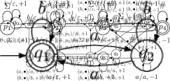
Figure 1: On the left, a 2DFT ${\mathcal{A}}$ with $[\![\mathcal{A}]\!](ba^{m_{1}}ba^{m_{2}}b\dots a^{m_{k}}b)=a^{m_{2}}b^{m_{1}}a^{m_{3}}b^{m_{2}}\dots a^{m_{k}}b^{m_{k-1}}$. On the right, an $\omega$-2DMT_la ${\mathcal{A}}^{\prime}$ with $[\![{\mathcal{A}}^{\prime}]\!](u_{1}\#u_{2}\#\dots\#u_{n}\#v)=u^{R}_{1}u_{1}\#u^{R}_{2}u_{2}\#\dots\#u^{R}_{n}u_{n}\#v$ where $u_{1},\dots,u_{n}\in(a+b)^{*}$, $v\in(a+b)^{\omega}$ and $u^{R}$ denotes the reverse of $u$. The Muller acceptance set is $\{\{q_{5}\}\}$. The look-ahead expressions $\Sigma^{*}\#\Sigma^{\omega}$ and $(\Sigma\backslash\{\#\})^{\omega}$ are used to check if there is a $\#$ in the remaining suffix of the input word.

In both cases of finite words and infinite words, we come up with a set of combinators using which, we form regular transducer expressions (RTE) characterizing the output of the two-way transducer (2DFT/$\omega$-2DMT_la).

The Combinators. We describe our basic combinators that form the building blocks of RTEs. The semantics of an RTE is a partial function $f\colon\Sigma^{\infty}\to\Gamma^{\infty}$ whose domain is denoted $\mathsf{dom}(f)$.

• We first look at the case of finite words and describe the basic combinators. The constant function is one which maps all strings in $\Sigma^{*}$ to some fixed value $d$. Given a string $w\in\Sigma^{*}$, the if-then-else combinator ${K}\,?\,{f}:{g}$ checks if $w$ is in the regular language $K$ or not, and appropriately produces $f(w)$ or $g(w)$. The unambiguous Cauchy product $f\boxdot g$ when applied on $w\in\Sigma^{*}$ produces $f(u)\cdot g(v)$ if $w=u\cdot v$ is an unambiguous decomposition of $w$ with $u\in\mathsf{dom}(f)$ and $v\in\mathsf{dom}(g)$. The unambiguous Kleene-plus $f^{\boxplus}$ when applied to $w\in\Sigma^{*}$ produces $f(u_{1})\cdots f(u_{n})$ if $w=u_{1}\cdots u_{n}$ is an unambiguous factorization of $w$, with each $u_{i}\in\mathsf{dom}(f)$. The Hadamard product $f\odot g$ when applied to $w$ produces $f(w)\cdot g(w)$. Finally, the unambiguous 2-chained Kleene-plus $[K,f]^{2\scriptstyle{\boxplus}}$ when applied to a string $w$ produces as output $f(u_{1}u_{2})\cdot f(u_{2}u_{3})\cdots f(u_{n-1}u_{n})$ if $w$ can be unambiguously written as $u_{1}u_{2}\cdots u_{n}$, with each $u_{i}\in K$, for the regular language $K$. We also have the reverses $f\mathbin{{\overleftarrow{\rule{0.0pt}{5.59721pt}\boxdot}}}g,{f}^{\scriptstyle{\overleftarrow{\rule{0.0pt}{3.91806pt}\boxplus}}}$ and $[K,f]^{\scriptstyle{\overleftarrow{\rule{0.0pt}{3.91806pt}2\boxplus}}}$: $[f\mathbin{{\overleftarrow{\rule{0.0pt}{5.59721pt}\boxdot}}}g](w)$ produces $g(v)\cdot f(u)$ if $w$ is the unambiguous concatenation $u\cdot v$ with $u\in\mathsf{dom}(f)$ and $v\in\mathsf{dom}(g)$, ${f}^{\scriptstyle{\overleftarrow{\rule{0.0pt}{3.91806pt}\boxplus}}}(w)$ produces $f(u_{n})\cdots f(u_{1})$ if $w$ is the unambiguous catenation $u_{1}\cdots u_{n}$ with $u_{i}\in\mathsf{dom}(f)$ for all $i$, and, $[K,f]^{\scriptstyle{\overleftarrow{\rule{0.0pt}{3.91806pt}2\boxplus}}}(w)$ produces $f(u_{n-1}u_{n})\cdots f(u_{1}u_{2})$ if $w$ is the unambiguous catenation $u_{1}\cdots u_{n}$ with $u_{i}\in K$ for all $i$.

• In the case of infinite words, the Cauchy product $f\boxdot g$ works on $w\in\Sigma^{\omega}$ if $w$ can be written unambiguously as $u\cdot v$ with $u\in\mathsf{dom}(f)\cap\Sigma^{*}$ and $v\in\mathsf{dom}(g)\cap\Sigma^{\omega}$. Another difference is in the use of the Hadamard product: for $w\in\Sigma^{\omega}$, $f\odot g$ produces $f(w)\cdot g(w)$ if $f(w)$ is a finite string. Note that these are sound with respect to the concatenation semantics for infinite words. Indeed, we also have $\omega$-iteration and two-chained $\omega$-iteration: $f^{\omega}(w)=f(u_{1})f(u_{2})\cdots$ if $w\in\Sigma^{\omega}$ can be unambiguously decomposed as $w=u_{1}u_{2}\cdots$ with $u_{i}\in\mathsf{dom}(f)\cap\Sigma^{*}$ for all $i\geq 1$. Moreover, $[K,f]^{2\omega}(w)=f(u_{1}u_{2})f(u_{2}u_{3})\cdots$ if $w\in\Sigma^{\omega}$ can be unambiguously decomposed as $w=u_{1}u_{2}\cdots$ with $u_{i}\in K$ for all $i\geq 1$, where $K\subseteq\Sigma^{*}$ is regular.

• An RTE is formed using all the above basic combinators.

• As an example, consider the RTE $C={{C_{4}}^{\scriptstyle{\boxplus}}\mathbin{{\boxdot}}C_{2}^{\omega}}$ with $C_{4}={((a+b)^{*}\#)}\,?\,{({C_{3}}^{\scriptstyle{\overleftarrow{\rule{0.0pt}{3.91806pt}\boxplus}}}\odot{C_{1}}^{\scriptstyle{\boxplus}})}:{\bot}$, $C_{2}={a}\,?\,{a}:{({b}\,?\,{b}:{\bot})}$. Here, $C_{1}={a}\,?\,{a}:{({b}\,?\,{b}:{({\#}\,?\,{\#}:{\bot})})}$, and $C_{3}={a}\,?\,{a}:{({b}\,?\,{b}:{({\#}\,?\,{\epsilon}:{\bot})})}$. Then $\mathsf{dom}(C_{1})=\mathsf{dom}(C_{3})=(a+b+\#)$, $\mathsf{dom}(C_{2})=(a+b)$, $\mathsf{dom}(C_{4})=(a+b)^{*}\#$ and, for $u\in(a+b)^{*}$, $[\![C_{4}]\!](u\#)=u^{R}u\#$ where $u^{R}$ denotes the reverse of $u$. This gives $\mathsf{dom}(C)=[(a+b)^{*}\#]^{+}(a+b)^{\omega}$ with $[\![C]\!](u_{1}\#u_{2}\#\cdots u_{n}\#v)=u_{1}^{R}u_{1}\#u_{2}^{R}u_{2}\#\cdots\#u_{n}^{R}u_{n}\#v$ when $u_{i}\in(a+b)^{*}$ and $v\in(a+b)^{\omega}$. The RTE $C^{\prime}={(a+b)^{\omega}}\,?\,{C_{2}^{\omega}}:{C}$ corresponds to the $\omega$-2DMT_la ${\mathcal{A}}^{\prime}$ in Figure 1; that is, $[\![C^{\prime}]\!]=[\![{\mathcal{A}}^{\prime}]\!]$.

• The combinators proposed in [5] also require unambiguity in concatenation and iteration. The base function $L/d$ in [5] maps all strings in language $L$ to the constant $d$, and is undefined for strings not in $L$. This can be written using our if-then-else ${L}\,?\,{d}:{\bot}$. The conditional choice combinator $f\triangleright g$ of [5] maps an input $\sigma$ to $f(\sigma)$ if it is in $dom(f)$, and otherwise it maps it to $g(\sigma)$. This can be written in our if-then-else as ${\mathsf{dom}(f)}\,?\,{f}:{g}$. The split-sum combinator $f\oplus g$ of [5] is our Cauchy product $f\boxdot g$. The iterated sum $\Sigma f$ of [5] is our Kleene-plus $f^{\boxplus}$. The left-split-sum and left-iterated sum of [5] are counterparts of our reverse Cauchy product $f\mathbin{{\overleftarrow{\rule{0.0pt}{5.59721pt}\boxdot}}}g$ and reverse Kleene-plus ${f}^{\scriptstyle{\overleftarrow{\rule{0.0pt}{3.91806pt}\boxplus}}}$. The sum $f+g$ of two functions in [5] is our Hadamard product $f\odot g$. Finally, the chained sum $\Sigma(f,L)$ of [5] is our two-chained Kleene-plus $[L,f]^{2\scriptstyle{\boxplus}}$. In our case, the terminology is all inspired from weighted automata literature, and the unambiguity comes from the use of the unambiguous factorization of the domain into good expressions, and we also extend our RTEs to infinite words.

Our main result is that two-way deterministic transducers and regular transducer expressions are effectively equivalent, both for finite and infinite words. See Appendix A.2 for a practical example using transducers.

Theorem 1.1.

(1) Given an RTE (resp. $\omega$-RTE) we can effectively construct an equivalent 2DFT (resp. an $\omega$-2DMT_la). Conversely, (2) given a 2DFT (resp. an $\omega$-2DMT_la) we can effectively construct an equivalent RTE (resp. $\omega$-RTE).

The proof of (1) is by structural induction on the RTE. The construction of an RTE starting from a two-way deterministic transducer ${\mathcal{A}}$ is quite involved. It is based on the transition monoid $\mathsf{TrM}({\mathcal{A}})$ of the transducer. This is a classical notion for two-way transducers over finite words, but not for two-way transducers with look-ahead on infinite words (to the best of our knowledge). So we introduce the notion of transition monoid for $\omega$-2DMT_la. We handle the look-ahead with a backward deterministic Büchi automaton ($\mathsf{BDBA}$), also called complete unambiguous or strongly unambiguous Büchi automata [7, 18]. The translation of ${\mathcal{A}}$ to an RTE is crucially guided by a “good” rational expression induced by the transition monoid of ${\mathcal{A}}$. These “good” expressions are obtained thanks to an unambiguous version [16] of the celebrated forest factorization theorem due to Imre Simon [17]. The unambiguous forest factorization theorem implies that, given a two-way transducer ${\mathcal{A}}$, any input word $w$ in the domain of ${\mathcal{A}}$ can be factorized unambiguously following a “good” rational expression induced by the transition monoid of ${\mathcal{A}}$. This unambiguous factorization then guides the construction of the RTE corresponding to ${\mathcal{A}}$. This algebraic backdrop facilitates a uniform treatment in the case of infinite words and finite words. As a remark, it is not apriori clear how the result of [5] extends to infinite words using the techniques therein.

Goodness of Rational Expressions. The goodness of a rational expression over alphabet $\Sigma$ is defined using a morphism $\varphi$ from $\Sigma^{*}$ to a monoid $(S,.,1_{S})$. A rational expression $F$ is good iff (i) it is unambiguous and (ii) for each subexpression $E$ of $F$, the image of all strings in $L(E)$ maps to a single monoid element $s_{E}$, and (iii) for each subexpression $E^{+}$ of $F$, $s_{E}$ is an idempotent. Note that unambiguity ensures the functionality of the output computed. Good rational expressions might be useful in settings beyond two-way transducers.

Computing the RTE. As an example, we now show how one computes an RTE equivalent to the 2DFT ${\mathcal{A}}$ on the left of Figure 1.

1. We work with the morphism $\mathsf{Tr}\colon\Sigma^{*}\to\mathsf{TrM}$ which maps words $w\in\Sigma^{*}$ to the transition monoid $\mathsf{TrM}$ of ${\mathcal{A}}$. An element $X\in\mathsf{TrM}$ is a set consisting of triples $(p,d,q)$, where $d$ is a direction $\{\mathrel{\leavevmode\resizebox{1.5pt}{0.8pt}{\rotatebox[origin={c}]{-90.0}{$\curvearrowright$}}},\mathrel{\leavevmode\resizebox{1.5pt}{0.8pt}{\rotatebox[origin={c}]{90.0}{$\curvearrowleft$}}},\rightarrow,\leftarrow\}$. Given a word $w\in\Sigma^{*}$, a triple $(p,\mathrel{\leavevmode\resizebox{1.5pt}{0.8pt}{\rotatebox[origin={c}]{-90.0}{$\curvearrowright$}}},q)\in\mathsf{Tr}(w)$ iff when starting in state $p$ on the left most symbol of $w$, the run of ${\mathcal{A}}$ leaves $w$ on the left in state $q$. The other directions $\mathrel{\leavevmode\resizebox{1.5pt}{0.8pt}{\rotatebox[origin={c}]{90.0}{$\curvearrowleft$}}}$ (start at the rightmost symbol of $w$ in state $p$ and leave $w$ on the right in state $q$), $\leftarrow$ and $\rightarrow$ are similar. In general, we have $w\in\mathsf{dom}({\mathcal{A}})$ iff on input ${\vdash}\,w\,{\dashv}$, starting on ${\vdash}$ in the initial state of ${\mathcal{A}}$, the run exits on the right of ${\dashv}$ in some final state of ${\mathcal{A}}$. With the automaton ${\mathcal{A}}$ on the left of Figure 1 we have $w\in\mathsf{dom}({\mathcal{A}})$ iff $(q_{0},\rightarrow,q_{2})\in\mathsf{Tr}(w)$.

2. For each $X\in\mathsf{TrM}$ such that $(q_{0},\rightarrow,q_{2})\in X$, we find an RTE $C_{X}$ whose domain is $\mathsf{Tr}^{-1}(X)$ and such that $[\![{\mathcal{A}}]\!](w)=[\![C_{X}]\!](w)$ for all $w\in\mathsf{Tr}^{-1}(X)$. The RTE corresponding to $[\![{\mathcal{A}}]\!]$ is the disjoint union of all these RTEs and is written using the if-then-else construct iterating over for all such elements $X$. For instance, if the monoid elements containing $(q_{0},\rightarrow,q_{2})$ are $X_{1},X_{2},X_{3}$ then we set $C={\mathsf{Tr}^{-1}(X_{1})}\,?\,{C_{X_{1}}}:{({\mathsf{Tr}^{-1}(X_{2})}\,?\,{C_{X_{2}}}:{({\mathsf{Tr}^{-1}(X_{3})}\,?\,{C_{X_{3}}}:{\bot})})}$ where $\bot$ stands for a nowhere defined function, i.e., $\mathsf{dom}(\bot)=\emptyset$.

3. Consider the language $L=(ba^{+})^{+}b\subseteq\mathsf{dom}({\mathcal{A}})$. Notice that the regular expression $(ba^{+})^{+}b$ is not “good”. For instance, condition (ii) is violated since $\mathsf{Tr}(bab)\neq\mathsf{Tr}(babab)$. Indeed, we can seen in Figure 2 that if we start on the right of $bab$ in state $q_{3}$ then we exist on the left in state $q_{5}$: $(q_{3},\leftarrow,q_{5})\in\mathsf{Tr}(bab)$. On the other hand, if we start on the right of $babab$ in state $q_{3}$ then we exist on the right in state $q_{2}$: $(q_{3},\mathrel{\leavevmode\resizebox{1.5pt}{0.8pt}{\rotatebox[origin={c}]{90.0}{$\curvearrowleft$}}},q_{2})\in\mathsf{Tr}(babab)$. Also, $(q_{5},\rightarrow,q_{1})\in\mathsf{Tr}(bab)$ while $(q_{5},\rightarrow,q_{2})\in\mathsf{Tr}(babab)$. It can be seen that $\mathsf{Tr}(a)$ is an idempotent, hence $\mathsf{Tr}(a^{+})=\mathsf{Tr}(a)$. We deduce also $\mathsf{Tr}(ba^{+}b)=\mathsf{Tr}(bab)$. Finally, we have $\mathsf{Tr}((ba^{+})^{n}b)=\mathsf{Tr}(babab)$ for all $n\geq 2$. Therefore, to obtain the RTE corresponding to $L$, we compute RTEs corresponding to $ba^{+}b$ and $(ba^{+})^{+}ba^{+}b$ satisfying conditions (i) and (ii) of “good” rational expressions.

4. While $ba^{+}b$ is good since $\mathsf{Tr}(a)$ is an idempotent, $(ba^{+})^{+}ba^{+}b$ is not good, the reason being that $\mathsf{Tr}(ba^{+})$ is not an idempotent. We can check that $\mathsf{Tr}(ba^{+}ba^{+})$ is still not idempotent, while $\mathsf{Tr}((ba^{+})^{i})=\mathsf{Tr}((ba^{+})^{3})$ for all $i\geq 3$, (see Figure 2: we only need to argue for $(q_{0},\rightarrow,q_{3}),(q_{5},\rightarrow,q_{3})$ and $(q_{6},\rightarrow,q_{3})$ in $\mathsf{Tr}((ba)^{i})$, $i\geq 3$, all other entries trivially carry over). In particular, $\mathsf{Tr}((ba^{+})^{3})$ is an idempotent. Thus, to compute the RTE for $L=(ba^{+})^{+}b$, we consider the RTEs corresponding to the “good” regular expressions $E_{1}=ba^{+}b$, $E_{2}=ba^{+}ba^{+}b$, $E_{3}=[(ba^{+})^{3}]^{+}b$, $E_{4}=[(ba^{+})^{3}]^{+}ba^{+}b$ and $E_{5}=[(ba^{+})^{3}]^{+}ba^{+}ba^{+}b$.

   

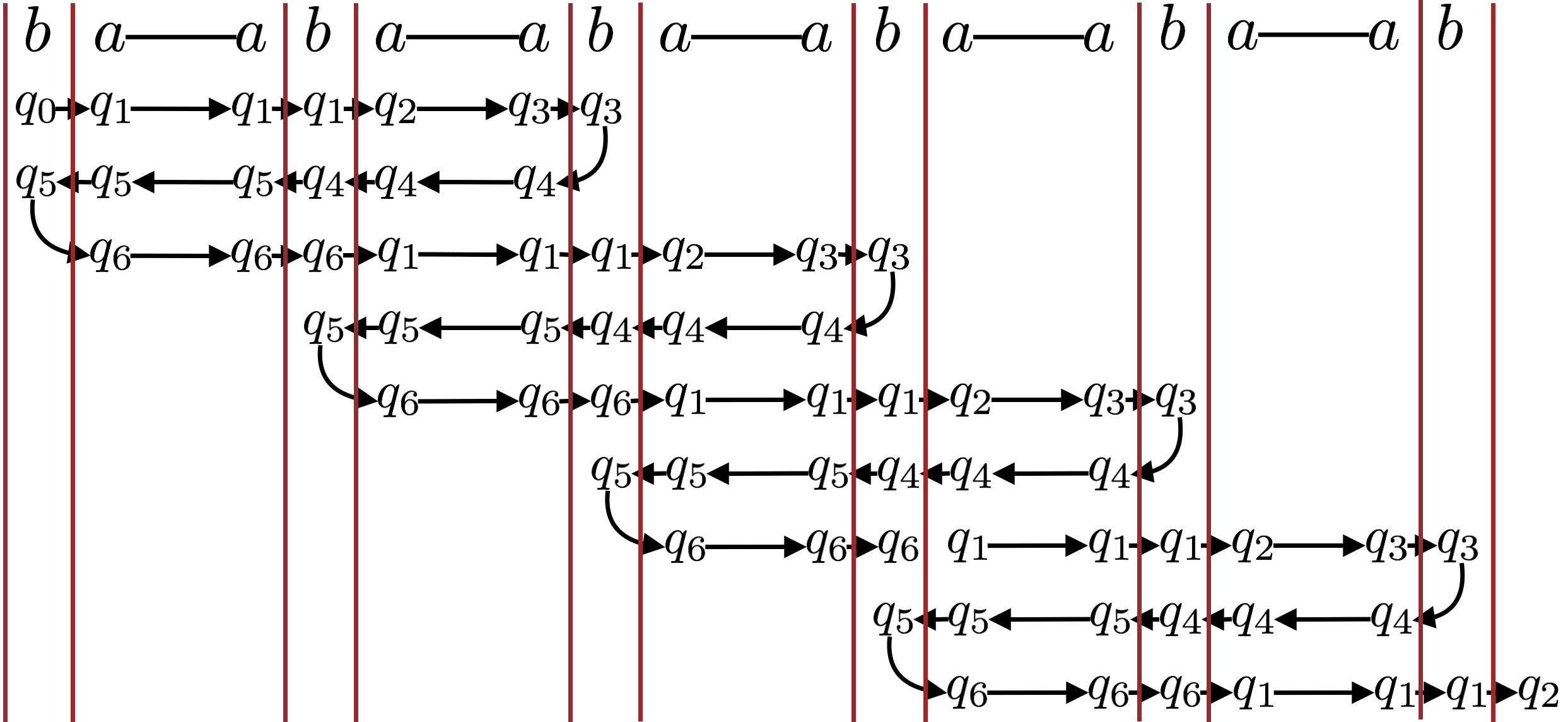
   Figure 2: Run of ${\mathcal{A}}$ on an input word in $(ba^{+})^{+}b$.

5. We define by induction, for each “good” expression $E$ and “step” $x=(p,d,q)$ in the monoid element $X=\mathsf{Tr}(E)$ associated with $E$, an RTE $C_{E}(x)$ whose domain is $E$ and, given a word $w\in E$, it computes $[\![C_{E}(x)]\!](w)$ the output of $\mathcal{A}$ when running step $x$ on $w$. For instance, if $E=a$ and $x=(q_{5},\leftarrow,q_{5})$ the output is $b$ so we set $C_{a}(q_{5},\leftarrow,q_{5})=({a}\,?\,{b}:{\bot})$. The if-then-else ensures that the domain is $a$. Similarly, we get the RTE associated with all atomic expressions and steps. For instance, $C_{b}(q_{1},\rightarrow,q_{2})=({b}\,?\,{\varepsilon}:{\bot})=C_{b}(q_{3},\mathrel{\leavevmode\resizebox{1.5pt}{0.8pt}{\rotatebox[origin={c}]{-90.0}{$\curvearrowright$}}},q_{4})$. For $u,v\in\Sigma^{*}$, we introduce the macro $u/v={u}\,?\,{v}:{\bot}$. We have $\mathsf{dom}(u/v)=\{u\}$ and $[\![u/v]\!](u)=v$.

   We turn to the good expression $a^{+}$. If we start on the right of a word $w\in a^{+}$ from state $q_{5}$ then we read the word from right to left using always the step $(q_{5},\leftarrow,q_{5})$. Therefore, we have $C_{a^{+}}(q_{5},\leftarrow,q_{5})={(C_{a}(q_{5},\leftarrow,q_{5}))}^{\scriptstyle{\overleftarrow{\rule{0.0pt}{3.91806pt}\boxplus}}}={(a/b)}^{\scriptstyle{\overleftarrow{\rule{0.0pt}{3.91806pt}\boxplus}}}$. Similarly, $C_{a^{+}}(q_{4},\leftarrow,q_{4})={(a/a)}^{\scriptstyle{\overleftarrow{\rule{0.0pt}{3.91806pt}\boxplus}}}$, $C_{a^{+}}(q_{1},\rightarrow,q_{1})={(a/\varepsilon)}^{\scriptstyle{\boxplus}}=C_{a^{+}}(q_{6},\rightarrow,q_{6})$. Now if we start on the left of a word $w\in a^{+}$ from state $q_{2}$ then we first take the step $(q_{2},\rightarrow,q_{3})$ and then we iterate the step $(q_{3},\rightarrow,q_{3})$. Therefore, we have $C_{a^{+}}(q_{2},\rightarrow,q_{3})={a}\,?\,{C_{a}(q_{2},\rightarrow,q_{3})}:{(C_{a}(q_{2},\rightarrow,q_{3})\mathbin{{\boxdot}}{(C_{a}(q_{3},\rightarrow,q_{3}))}^{\scriptstyle{\boxplus}})}={a}\,?\,{(a/\varepsilon)}:{\big{(}(a/\varepsilon)\mathbin{{\boxdot}}{(a/\varepsilon)}^{\scriptstyle{\boxplus}}\big{)}}$, which is equivalent to the RTE ${(a/\varepsilon)}^{\scriptstyle{\boxplus}}$.

   We consider now $E=ba^{+}ba^{+}$ and the step $x=(q_{0},\rightarrow,q_{3})$. We have (see Figure 2)

   $$C_{E}(x) =C_{b}(q_{0},\rightarrow,q_{1})\mathbin{{\boxdot}}C_{a^{+}}(q_{1},\rightarrow,q_{1})\mathbin{{\boxdot}}C_{b}(q_{1},\rightarrow,q_{2})\mathbin{{\boxdot}}C_{a^{+}}(q_{2},\rightarrow,q_{3})$$

   $$=(b/\varepsilon)\mathbin{{\boxdot}}{(a/\varepsilon)}^{\scriptstyle{\boxplus}}\mathbin{{\boxdot}}(b/\varepsilon)\mathbin{{\boxdot}}{(a/\varepsilon)}^{\scriptstyle{\boxplus}}$$

   $$\approx({ba^{+}ba^{+}}\,?\,{\varepsilon}:{\bot})\,.$$

   More interesting is the step $y=(q_{4},\mathrel{\leavevmode\resizebox{1.5pt}{0.8pt}{\rotatebox[origin={c}]{90.0}{$\curvearrowleft$}}},q_{1})$ since on a word $w\in E$, the run which starts on the right in state $q_{4}$ goes all the way to the left until it reads the first $b$ in state $q_{5}$ and then moves to the right until it exists in state $q_{1}$ (see Figure 2). Therefore, we have

   $$C_{E}(y) =\big{(}(b/\varepsilon)\mathbin{{\overleftarrow{\rule{0.0pt}{5.59721pt}\boxdot}}}C_{a^{+}}(q_{5},\leftarrow,q_{5})\mathbin{{\overleftarrow{\rule{0.0pt}{5.59721pt}\boxdot}}}C_{b}(q_{4},\leftarrow,q_{5})\mathbin{{\overleftarrow{\rule{0.0pt}{5.59721pt}\boxdot}}}C_{a^{+}}(q_{4},\leftarrow,q_{4})\big{)}\odot{}$$

   $$\hskip 11.38109pt\big{(}C_{b}(q_{5},\rightarrow,q_{6})\mathbin{{\boxdot}}C_{a^{+}}(q_{6},\rightarrow,q_{6})\mathbin{{\boxdot}}C_{b}(q_{6},\rightarrow,q_{1})\mathbin{{\boxdot}}C_{a^{+}}(q_{1},\rightarrow,q_{1})\big{)}$$

   $$=\big{(}(b/\varepsilon)\mathbin{{\overleftarrow{\rule{0.0pt}{5.59721pt}\boxdot}}}{(a/b)}^{\scriptstyle{\overleftarrow{\rule{0.0pt}{3.91806pt}\boxplus}}}\mathbin{{\overleftarrow{\rule{0.0pt}{5.59721pt}\boxdot}}}(b/\varepsilon)\mathbin{{\overleftarrow{\rule{0.0pt}{5.59721pt}\boxdot}}}{(a/a)}^{\scriptstyle{\overleftarrow{\rule{0.0pt}{3.91806pt}\boxplus}}}\big{)}\odot\big{(}(b/\varepsilon)\mathbin{{\boxdot}}{(a/\varepsilon)}^{\scriptstyle{\boxplus}}\mathbin{{\boxdot}}(b/\varepsilon)\mathbin{{\boxdot}}{(a/\varepsilon)}^{\scriptstyle{\boxplus}}\big{)}$$

   $$\approx(b/\varepsilon)\mathbin{{\overleftarrow{\rule{0.0pt}{5.59721pt}\boxdot}}}{(a/b)}^{\scriptstyle{\overleftarrow{\rule{0.0pt}{3.91806pt}\boxplus}}}\mathbin{{\overleftarrow{\rule{0.0pt}{5.59721pt}\boxdot}}}(b/\varepsilon)\mathbin{{\overleftarrow{\rule{0.0pt}{5.59721pt}\boxdot}}}{(a/a)}^{\scriptstyle{\overleftarrow{\rule{0.0pt}{3.91806pt}\boxplus}}}\,.$$

   The leftmost $(b/\varepsilon)$ in the first line is used to make sure that the input word belongs to $E=ba^{+}ba^{+}$. Composing these steps on the right with $b$, we obtain the RTE $C_{2}=C_{E_{2}}(q_{0},\rightarrow,q_{2})$ which describes the behaviour of ${\mathcal{A}}$ on the subset $E_{2}=ba^{+}ba^{+}b\subseteq\mathsf{dom}({\mathcal{A}})$:

   $$C_{2} =\big{(}C_{E}(x)\mathbin{{\boxdot}}C_{b}(q_{3},\mathrel{\leavevmode\resizebox{1.5pt}{0.8pt}{\rotatebox[origin={c}]{-90.0}{$\curvearrowright$}}},q_{4})\big{)}\odot\big{(}C_{E}(y)\mathbin{{\boxdot}}C_{b}(q_{1},\rightarrow,q_{2})\big{)}$$

   $$=\big{(}C_{E}(x)\mathbin{{\boxdot}}(b/\varepsilon)\big{)}\odot\big{(}C_{E}(y)\mathbin{{\boxdot}}(b/\varepsilon)\big{)}$$

   $$\approx\big{(}(b/\varepsilon)\mathbin{{\overleftarrow{\rule{0.0pt}{5.59721pt}\boxdot}}}{(a/b)}^{\scriptstyle{\overleftarrow{\rule{0.0pt}{3.91806pt}\boxplus}}}\mathbin{{\overleftarrow{\rule{0.0pt}{5.59721pt}\boxdot}}}(b/\varepsilon)\mathbin{{\overleftarrow{\rule{0.0pt}{5.59721pt}\boxdot}}}{(a/a)}^{\scriptstyle{\overleftarrow{\rule{0.0pt}{3.91806pt}\boxplus}}}\big{)}\mathbin{{\boxdot}}(b/\varepsilon)\,.$$

   Therefore, $[\![C_{2}]\!](ba^{m_{1}}ba^{m_{2}}b)=a^{m_{2}}b^{m_{1}}=[\![{\mathcal{A}}]\!](ba^{m_{1}}ba^{m_{2}}b)$.

   In Appendix A.1, we show the computation of the RTE $C_{E_{3}}(q_{0},\rightarrow,q_{2})$ for $E_{3}=[(ba^{+})^{3}]^{+}b\subseteq\mathsf{dom}({\mathcal{A}})$.

2 Finite Words

We start with the definition of two-way automata and transducers for the case of finite words.

2.1 Two-way automata and transducers

Let $\Sigma$ be a finite input alphabet and let ${\vdash},{\dashv}$ be two special symbols not in $\Sigma$. We assume that every input string $w\in\Sigma^{*}$ is presented as ${\vdash}w{\dashv}$, where ${\vdash},{\dashv}$ serve as left and right delimiters that appear nowhere else in $w$. We write $\Sigma_{{\vdash}{\dashv}}=\Sigma\cup\{{\vdash},{\dashv}\}$. A two-way automaton ${\mathcal{A}}=(Q,\Sigma,\delta,I,F)$ has a finite set of states $Q$, subsets $I,F\subseteq Q$ of initial and final states and a transition relation $\delta\subseteq Q\times\Sigma_{{\vdash}{\dashv}}\times Q\times\{-1,1\}$. The -1 represents the reading head moving to the left, while a 1 represents the reading head moving to the right. The reading head cannot move left when it is on ${\vdash}$. A configuration of ${\mathcal{A}}$ is represented by $w_{1}qw_{2}$ where $q\in Q$ and $w_{1}w_{2}\in{{\vdash}\Sigma^{*}{\dashv}}$. If $w_{2}=\varepsilon$ the computation has come to an end. Otherwise, the reading head of ${\mathcal{A}}$ is scanning the first symbol of $w_{2}\neq\varepsilon$ in state $q$. If $w_{2}=aw^{\prime}_{2}$ and if $(q,a,q^{\prime},-1)\in\delta$ (hence $a\neq{\vdash}$), then there is a transition from the configuration $w^{\prime}_{1}bqaw^{\prime}_{2}$ to $w^{\prime}_{1}q^{\prime}baw^{\prime}_{2}$. Likewise, if $(q,a,q^{\prime},1)\in\delta$, we obtain a transition from $w_{1}qaw^{\prime}_{2}$ to $w_{1}aq^{\prime}w^{\prime}_{2}$. A run of ${\mathcal{A}}$ is a sequence of transitions; it is accepting if it starts in a configuration $p{\vdash}w{\dashv}$ with $p\in I$ and ends in a configuration ${\vdash}w{\dashv}q$ with $q\in F$. The language $\mathcal{L}({\mathcal{A}})$ or domain $\mathsf{dom}({\mathcal{A}})$ of ${\mathcal{A}}$ is the set of all words $w\in\Sigma^{*}$ which have an accepting run in ${\mathcal{A}}$.

To extend the definition of a two-way automaton ${\mathcal{A}}$ into a two-way transducer, $(Q,\Sigma,\delta,I,F)$ is extended to $(Q,\Sigma,\Gamma,\delta,I,F)$ by adding a finite output alphabet $\Gamma$ and the definition of the transition relation as a finite subset $\delta\subseteq Q\times\Sigma_{{\vdash}{\dashv}}\times Q\times\Gamma^{*}\times\{-1,1\}$. The output produced on each transition is appended to the right of the output produced so far. ${\mathcal{A}}$ defines a relation $[\![{\mathcal{A}}]\!]=\{(u,w)\mid u\in\mathcal{L}({\mathcal{A}})$ and $w$ is the output produced on an accepting run of $u\}$.

The transducer ${\mathcal{A}}$ is said to be functional if for each input $u\in\mathsf{dom}({\mathcal{A}})$, at most one output $w$ can be produced. In this case, for each $u\in\mathsf{dom}({\mathcal{A}})$ in the domain, there is exactly one $w\in\Gamma^{*}$ such that $(u,w)\in[\![{\mathcal{A}}]\!]$. We also denote this by $[\![{\mathcal{A}}]\!](u)=w$. We consider a special symbol $\bot\notin\Gamma$ that will stand for undefined. We let $[\![{\mathcal{A}}]\!](u)=\bot$ when $u\notin\mathsf{dom}({\mathcal{A}})$. Thus, the semantics of a functional transducer ${\mathcal{A}}$ is a map $[\![{\mathcal{A}}]\!]\colon\Sigma^{*}\to\mathbb{D}=\Gamma^{*}\cup\{\bot\}$ such that $u\in\mathsf{dom}({\mathcal{A}})$ iff $[\![{\mathcal{A}}]\!](u)\neq\bot$.

We use non-deterministic unambiguous two-way transducers (2NUFT) in some proofs. A two-way transducer is unambiguous if each string $u\in\Sigma^{*}$ has at most one accepting run. Clearly, 2NUFTs are functional. A deterministic two-way transducer (2DFT) is one having a single initial state and where, from each state, on each symbol $a\in\Sigma_{{\vdash}{\dashv}}$, at most one transition is enabled. In that case, the transition relation is a partial function $\delta\colon Q\times\Sigma_{{\vdash}{\dashv}}\to Q\times\Gamma^{*}\times\{-1,1\}$. 2DFTs are by definition unambiguous. It is known [8] that 2DFTs are equivalent to 2NUFTs.

A 1DFT (1NUFT) represents a deterministic (non-deterministic unambiguous) transducer where the reading head only moves to the right.

Example 2.1.

On the left of Figure 1, a two-way transducer $\mathcal{A}$ is given with $\mathsf{dom}(\mathcal{A})=(ba^{*})^{+}b$, $[\![\mathcal{A}]\!](ba^{m_{1}}b)=\varepsilon$ and $[\![\mathcal{A}]\!](ba^{m_{1}}ba^{m_{2}}b\cdots a^{m_{k}}b)=a^{m_{2}}b^{m_{1}}a^{m_{3}}b^{m_{2}}\cdots a^{m_{k}}b^{m_{k-1}}$ for $k\geq 2$.

2.2 Regular Transducer Expressions

Let $\Sigma$ and $\Gamma$ be finite input and output alphabets. Recall that $\bot\notin\Gamma$ is a special symbol that stands for undefined. We define the output monoid as $\mathbb{D}=\Gamma^{*}\cup\{\bot\}$ with the usual concatenation on words, $\bot$ acting as a zero: $d\cdot\bot=\bot\cdot d=\bot$ for all $d\in\mathbb{D}$. The unit is the empty word ${\mathbf{1}_{\mathbb{D}}}=\varepsilon$.

We define Regular Transducer Expressions (RTE) from $\Sigma^{*}$ to $\mathbb{D}$ using some basic combinators. The syntax of RTE is defined with the following grammar:

$$C::=d\mid{K}\,?\,{C}:{C}\mid C\odot C\mid C\mathbin{{\boxdot}}C\mid C\mathbin{{\overleftarrow{\rule{0.0pt}{5.59721pt}\boxdot}}}C\mid{C}^{\scriptstyle{\boxplus}}\mid{C}^{\scriptstyle{\overleftarrow{\rule{0.0pt}{3.91806pt}\boxplus}}}\mid[K,C]^{2\scriptstyle{\boxplus}}\mid[K,C]^{\scriptstyle{\overleftarrow{\rule{0.0pt}{3.91806pt}2\boxplus}}}$$

where $d\in\mathbb{D}$ ranges over output values, and $K\subseteq\Sigma^{*}$ ranges over regular languages of finite words. The semantics of an RTE $C$ is a function $[\![C]\!]\colon\Sigma^{*}\to\mathbb{D}$ defined inductively following the syntax of the expression, starting from constant functions. Since $\bot$ stands for undefined, we define the domain of a function $f\colon\Sigma^{*}\to\mathbb{D}$ by $\mathsf{dom}(f)=f^{-1}(\mathbb{D}\setminus\{\bot\})=\Sigma^{*}\setminus f^{-1}(\bot)$.

Constants.

For $d\in\mathbb{D}$, we let $[\![d]\!]$ be the constant map defined by $[\![d]\!](w)=d$ for all $w\in\Sigma^{*}$.

We have $\mathsf{dom}([\![d]\!])=\Sigma^{*}$ if $d\neq\bot$ and $\mathsf{dom}([\![\bot]\!])=\emptyset$.

Each regular combinator defined above allows to combine functions from $\Sigma^{*}$ to $\mathbb{D}$. For functions $f,g\colon\Sigma^{*}\to\mathbb{D}$, $w\in\Sigma^{*}$ and a regular language $K\subseteq\Sigma^{*}$, we define the following combinators.

If then else.

$({K}\,?\,{f}:{g})(w)$ is defined as $f(w)$ for $w\in K$, and $g(w)$ for $w\notin K$.

We have $\mathsf{dom}({K}\,?\,{f}:{g})=(\mathsf{dom}(f)\cap K)\cup(\mathsf{dom}(g)\setminus K)$.

Hadamard product.

$(f\odot g)(w)=f(w)\cdot g(w)$ (recall that $(\mathbb{D},\cdot,{\mathbf{1}_{\mathbb{D}}})$ is a monoid).

We have $\mathsf{dom}(f\odot g)=\mathsf{dom}(f)\cap\mathsf{dom}(g)$.

Unambiguous Cauchy product and its reverse.

If $w$ admits a unique factorization $w=u\cdot v$ with $u\in\mathsf{dom}(f)$ and $v\in\mathsf{dom}(g)$ then we set $(f\mathbin{{\boxdot}}g)(w)=f(u)\cdot g(v)$ and $(f\mathbin{{\overleftarrow{\rule{0.0pt}{5.59721pt}\boxdot}}}g)(w)=g(v)\cdot f(u)$. Otherwise, we set $(f\mathbin{{\boxdot}}g)(w)=\bot=(f\mathbin{{\overleftarrow{\rule{0.0pt}{5.59721pt}\boxdot}}}g)(w)$.

We have $\mathsf{dom}(f\mathbin{{\boxdot}}g)=\mathsf{dom}(f\mathbin{{\overleftarrow{\rule{0.0pt}{5.59721pt}\boxdot}}}g)\subseteq\mathsf{dom}(f)\cdot\mathsf{dom}(g)$ and the inclusion is strict if the concatenation of $\mathsf{dom}(f)$ and $\mathsf{dom}(g)$ is ambiguous.

Unambiguous Kleene-plus and its reverse.

If $w$ admits a unique factorization $w=u_{1}\cdot u_{2}\cdots u_{n}$ with $n\geq 1$ and $u_{i}\in\mathsf{dom}(f)$ for all $1\leq i\leq n$ then we set ${f}^{\scriptstyle{\boxplus}}(w)=f(u_{1})\cdot f(u_{2})\cdots f(u_{n})$ and ${f}^{\scriptstyle{\overleftarrow{\rule{0.0pt}{3.91806pt}\boxplus}}}(w)=f(u_{n})\cdots f(u_{2})\cdot f(u_{1})$. Otherwise, we set ${f}^{\scriptstyle{\boxplus}}(w)=\bot={f}^{\scriptstyle{\overleftarrow{\rule{0.0pt}{3.91806pt}\boxplus}}}(w)$.

We have $\mathsf{dom}({f}^{\scriptstyle{\boxplus}})=\mathsf{dom}({f}^{\scriptstyle{\overleftarrow{\rule{0.0pt}{3.91806pt}\boxplus}}})\subseteq\mathsf{dom}(f)^{+}$ and the inclusion is strict if the Kleene iteration $\mathsf{dom}(f)^{+}$ of $\mathsf{dom}(f)$ is ambiguous. Notice that $\mathsf{dom}({f}^{\scriptstyle{\boxplus}})=\emptyset$ when $\varepsilon\in\mathsf{dom}(f)$.

Unambiguous 2-chained Kleene-plus and its reverse.

If $w$ admits a unique factorization $w=u_{1}\cdot u_{2}\cdots u_{n}$ with $n\geq 1$ and $u_{i}\in K$ for all $1\leq i\leq n$ then we set $[K,f]^{2\scriptstyle{\boxplus}}(w)=f(u_{1}u_{2})\cdot f(u_{2}u_{3})\cdots f(u_{n-1}u_{n})$ and $[K,f]^{\scriptstyle{\overleftarrow{\rule{0.0pt}{3.91806pt}2\boxplus}}}(w)=f(u_{n-1}u_{n})\cdots f(u_{2}u_{3})\cdot f(u_{1}u_{2})$ (if $n=1$, the empty product gives the unit of $\mathbb{D}$: $[K,f]^{2\scriptstyle{\boxplus}}(w)={\mathbf{1}_{\mathbb{D}}}=[K,f]^{\scriptstyle{\overleftarrow{\rule{0.0pt}{3.91806pt}2\boxplus}}}(w)$). Otherwise, we set $[K,f]^{2\scriptstyle{\boxplus}}(w)=\bot=[K,f]^{\scriptstyle{\overleftarrow{\rule{0.0pt}{3.91806pt}2\boxplus}}}(w)$.

Again, we have $\mathsf{dom}([K,f]^{2\scriptstyle{\boxplus}})=\mathsf{dom}([K,f]^{\scriptstyle{\overleftarrow{\rule{0.0pt}{3.91806pt}2\boxplus}}})\subseteq K^{+}$ and the inclusion is strict if the Kleene iteration $K^{+}$ of $K$ is ambiguous. Notice that, even if $w\in K^{+}$ admits a unique factorization $w=u_{1}\cdot u_{2}\cdots u_{n}$ with $u_{i}\in K$ for all $1\leq i\leq n$, $w$ is not necessarily in the domain of $[K,f]^{2\scriptstyle{\boxplus}}$ or $[K,f]^{\scriptstyle{\overleftarrow{\rule{0.0pt}{3.91806pt}2\boxplus}}}$. For $w$ to be in this domain, it is further required that $u_{1}u_{2},u_{2}u_{3},\ldots,u_{n-1}u_{n}\in\mathsf{dom}(f)$. Notice that we have $\mathsf{dom}([K,f]^{2\scriptstyle{\boxplus}})=\mathsf{dom}([K,f]^{\scriptstyle{\overleftarrow{\rule{0.0pt}{3.91806pt}2\boxplus}}})=K^{+}$ when $K^{+}$ is unambiguous and $K^{2}\subseteq\mathsf{dom}(f)$.

Lemma 2.2.

The domain of an RTE $C$ is a regular language $\mathsf{dom}(C)\subseteq\Sigma^{*}$.

Remark 2.3.

Notice that the reverse Cauchy product is redundant, it can be expressed with the Hadamard product and the Cauchy product:

$$f\mathbin{{\overleftarrow{\rule{0.0pt}{5.59721pt}\boxdot}}}g=(({\mathsf{dom}(f)}\,?\,{\varepsilon}:{\bot})\mathbin{{\boxdot}}g)\odot(f\mathbin{{\boxdot}}({\mathsf{dom}(g)}\,?\,{\varepsilon}:{\bot}))\,.$$

The unambiguous Kleene-plus is also redundant, it can be expressed with the unambiguous 2-chained Kleene-plus:

$${f}^{\scriptstyle{\boxplus}}=[\mathsf{dom}(f),f\mathbin{{\boxdot}}({\mathsf{dom}(f)}\,?\,{\varepsilon}:{\bot})]^{2\scriptstyle{\boxplus}}\odot({(\mathsf{dom}(f)^{*}}\,?\,{\varepsilon}:{\bot})\mathbin{{\boxdot}}f)\,.$$

Example 2.4.

Consider the RTEs $C_{1}{=}{({[(a+b)^{+}\#]}\,?\,{\varepsilon}:{\bot}){\mathbin{{\boxdot}}}({(a+b)^{+}}\,?\,{\mathsf{copy}}:{\bot})}$, $C_{2}=\#$ and $C_{3}=({(a+b)^{+}}\,?\,{\mathsf{copy}}:{\bot}){\mathbin{{\boxdot}}}({[\#(a+b)^{+}]}\,?\,{\varepsilon}:{\bot})$, where $\mathsf{copy}={({a}\,?\,{a}:{(}{b}\,?\,{b}:{\bot}))}^{\scriptstyle{\boxplus}}$. Then, $\mathsf{dom}([\![C_{2}]\!])=\Sigma^{*}$, $\mathsf{dom}([\![\mathsf{copy}]\!])=(a+b)^{+}$ and $\mathsf{dom}([\![C_{1}]\!])=\mathsf{dom}([\![C_{3}]\!])=(a+b)^{+}\#(a+b)^{+}$. Moreover, $[\![C_{1}\odot C_{2}\odot C_{3}]\!](u\#v)=v\#u$ for all $u,v\in(a+b)^{+}$.

Example 2.5.

Consider the RTEs $C_{a}=({b}\,?\,{\varepsilon}:{\bot})\mathbin{{\boxdot}}{({a}\,?\,{a}:{\bot})}^{\scriptstyle{\boxplus}}$ and $C_{b}=({b}\,?\,{\varepsilon}:{\bot})\mathbin{{\boxdot}}{({a}\,?\,{b}:{\bot})}^{\scriptstyle{\boxplus}}$. We have $\mathsf{dom}([\![C_{a}]\!])=ba^{+}=\mathsf{dom}([\![C_{b}]\!])$ and $[\![C_{a}]\!](ba^{n})=a^{n}$ and $[\![C_{b}]\!](ba^{n})=b^{n}$. We deduce that $\mathsf{dom}([\![C_{b}\mathbin{{\overleftarrow{\rule{0.0pt}{5.59721pt}\boxdot}}}C_{a}]\!])=ba^{+}ba^{+}$ and $[\![C_{b}\mathbin{{\overleftarrow{\rule{0.0pt}{5.59721pt}\boxdot}}}C_{a}]\!](ba^{n}ba^{m})=a^{m}b^{n}$.

Consider the expression $C=[ba^{+},C_{b}\mathbin{{\overleftarrow{\rule{0.0pt}{5.59721pt}\boxdot}}}C_{a}]^{2\scriptstyle{\boxplus}}\mathbin{{\boxdot}}({b}\,?\,{\varepsilon}:{\bot})$. Then, $\mathsf{dom}([\![C]\!])=(ba^{+})^{+}b$, $[\![C]\!](ba^{m}b)=\varepsilon$ and $[\![C]\!](ba^{m_{1}}ba^{m_{2}}b\cdots a^{m_{k}}b)=a^{m_{2}}b^{m_{1}}a^{m_{3}}b^{m_{2}}\cdots a^{m_{k}}b^{m_{k-1}}$ for $k\geq 2$.

Theorem 2.6.

2DFTs and RTEs define the same class of functions. More precisely,

1. given an RTE $C$, we can construct a 2DFT $\mathcal{A}$ such that $[\![\mathcal{A}]\!]=[\![C]\!]$,

2. given a 2DFT $\mathcal{A}$, we can construct an RTE C such that $[\![\mathcal{A}]\!]=[\![C]\!]$.

The proof of (1) is given in the next section, while the proof of (2) will be given in Section 2.6 after some preliminaries in Section 2.5 on transition monoids for 2DFTs and the unambiguous forest factorization theorem.

2.3 RTE to 2DFT

In this section, we prove Theorem 2.6(1), i.e., we show that given an RTE $C$, we can construct a 2DFT ${\mathcal{A}}$ such that $[\![{\mathcal{A}}]\!]=[\![C]\!]$. We do this by structural induction on RTEs, starting with constant functions, and then later showing that 2DFTs are closed under all the combinators used in RTEs.

Constant functions: We start with the constant function $d\in\mathbb{D}$ for which it is easy to construct a 2DFT ${\mathcal{A}}$ such that $[\![d]\!]=[\![{\mathcal{A}}]\!]$. For $d=\bot$, we take ${\mathcal{A}}$ such that $\mathsf{dom}({\mathcal{A}})=\emptyset$ (for instance we use a single state and an empty transition function). Assume now that $d\in\Gamma^{*}$. The 2DFT scans the word up to the right end marker, outputs $d$ and stops. Formally, we let ${\mathcal{A}}=(\{q\},\Sigma,\Gamma,\delta,q,\{q\})$ s.t. $\delta(q,a)=(q,\varepsilon,+1)$ for all $a\in\Sigma\cup\{{\vdash}\}$ and $\delta(q,{\dashv})=(q,d,+1)$. Clearly, $[\![{\mathcal{A}}]\!](w)=d$ for all $w\in\Sigma^{*}$.

The inductive steps follow directly from:

Lemma 2.7.

Let $K\subseteq\Sigma^{*}$ be regular, and let $f$ and $g$ be RTEs with $[\![f]\!]=[\![M_{f}]\!]$ and $[\![g]\!]=[\![M_{g}]\!]$ for 2DFTs $M_{f}$ and $M_{g}$ respectively. Then, one can construct

1. a 2DFT ${\mathcal{A}}$ such that $[\![{K}\,?\,{f}:{g}]\!]=[\![{\mathcal{A}}]\!]$.

2. a 2DFT ${\mathcal{A}}$ such that $[\![{\mathcal{A}}]\!]=[\![f\odot g]\!]$.

3. 2DFTs ${\mathcal{A}}$, ${\mathcal{B}}$ such that $[\![{\mathcal{A}}]\!]=[\![f\mathbin{{\boxdot}}g]\!]$ and $[\![{\mathcal{B}}]\!]=[\![f\mathbin{{\overleftarrow{\rule{0.0pt}{5.59721pt}\boxdot}}}g]\!]$.

4. 2DFTs ${\mathcal{A}}$, ${\mathcal{B}}$ such that $[\![{\mathcal{A}}]\!]=[\![{f}^{\scriptstyle{\boxplus}}]\!]$ and $[\![{\mathcal{B}}]\!]=[\![{f}^{\scriptstyle{\overleftarrow{\rule{0.0pt}{3.91806pt}\boxplus}}}]\!]$.

5. 2DFTs ${\mathcal{A}}$, ${\mathcal{B}}$ such that $[\![{\mathcal{A}}]\!]=[\![[K,f]^{2\scriptstyle{\boxplus}}]\!]$ and $[\![{\mathcal{B}}]\!]=[\![[K,f]^{\scriptstyle{\overleftarrow{\rule{0.0pt}{3.91806pt}2\boxplus}}}]\!]$.

Proof 2.8.

(1) If then else. Let $\mathcal{B}$ be a complete DFA that accepts the regular language $K$. The idea of the proof is to construct a 2DFT ${\mathcal{A}}$ which first runs $\mathcal{B}$ on the input $w$ until the end marker ${\dashv}$ is reached in some state $q$ of $\mathcal{B}$. Then, $w\in K$ iff $q\in F$ is some accepting state of $\mathcal{B}$. The automaton ${\mathcal{A}}$ moves left all the way to ${\vdash}$, and starts running either $M_{f}$ or $M_{g}$ depending on whether $q\in F$ or not. Since $\mathcal{B}$ is complete, it is clear that $\mathsf{dom}({\mathcal{A}})=\mathsf{dom}({K}\,?\,{f}:{g})$ and the output of ${\mathcal{A}}$ coincides with $[\![M_{f}]\!]$ iff the input is in $K$, and otherwise coincides with $[\![M_{g}]\!]$.

(2) Hadamard product. Given an input $w$, the constructed 2DFT ${\mathcal{A}}$ first runs $M_{f}$. Instead of executing a transition $p\xrightarrow{{\dashv}/\gamma,+1}q$ with $q$ a final state of $M_{f}$, it executes $p\xrightarrow{{\dashv}/\gamma,-1}\mathsf{reset}$ where $\mathsf{reset}$ is a new state. While in the $\mathsf{reset}$ state, it moves all the way back to ${\vdash}$ and it starts running $M_{g}$ by executing $\mathsf{reset}\xrightarrow{{\vdash}/\gamma^{\prime},+1}q^{\prime}$ if $\delta_{g}(q_{0},{\vdash})=(q^{\prime},\gamma^{\prime},+1)$ where $\delta_{g}$ is the transition function of $M_{g}$ and $q_{0}$ is the initial state of $M_{g}$. The final states of ${\mathcal{A}}$ are those of $M_{g}$, and its initial state is the initial state of $M_{f}$. Clearly, $\mathsf{dom}({\mathcal{A}})=\mathsf{dom}(M_{f})\cap\mathsf{dom}(M_{g})$ and the output of ${\mathcal{A}}$ is the concatenation of the outputs of $M_{f}$ and $M_{g}$.

(3) Cauchy product. The domain of a 2DFT is a regular language, accepted by the 2DFA obtained by ignoring the outputs. Since 2DFAs are effectively equivalent to (1)DFAs, we can construct from $M_{f}$ and $M_{g}$ two DFAs $\mathcal{C}_{f}=(Q_{f},\Sigma,\delta_{f},s_{f},F_{f})$ and $\mathcal{C}_{g}=(Q_{g},\Sigma,\delta_{g},s_{g},F_{g})$ such that $\mathcal{L}(\mathcal{C}_{f})=\mathsf{dom}(f)$ and $\mathcal{L}(\mathcal{C}_{g})=\mathsf{dom}(g)$.

Now, the set $K$ of words $w$ having at least two factorizations $w=u_{1}v_{1}=u_{2}v_{2}$ with $u_{1},u_{2}\in\mathsf{dom}(f)$, $v_{1},v_{2}\in\mathsf{dom}(g)$ and $u_{1}\neq u_{2}$ is also regular. This is easy since $K$ can be written as $K=\bigcup_{p\in F_{f},q\in Q_{g}}L_{p}\cdot M_{p,q}\cdot R_{q}$ where

• $L_{p}$ is the set of words which admit a run in $\mathcal{C}_{f}$ from its initial state to the final state $p\in F_{f}$,

• $M_{p,q}$ is the set of words which admit a run in $\mathcal{C}_{f}$ from state $p$ to some final state in $F_{f}$, and also admit a run in $\mathcal{C}_{g}$ from its initial state to state $q\in Q_{g}$,

• $R_{q}$ is the set of words which admit a run in $\mathcal{C}_{g}$ from state $q$ to some final state in $F_{g}$, and also admit a run in $\mathcal{C}_{g}$ from its initial state to some final state in $F_{g}$.

Therefore, we have $\mathsf{dom}(f\mathbin{{\boxdot}}g)=\mathsf{dom}(f\mathbin{{\overleftarrow{\rule{0.0pt}{5.59721pt}\boxdot}}}g)=(\mathsf{dom}(f)\cdot\mathsf{dom}(g))\setminus K$ is a regular language and we construct a complete DFA $\mathcal{C}=(Q,\Sigma,\delta,q_{0},F)$ which accepts this language.

1. From $\mathcal{C}_{f}$, $\mathcal{C}_{g}$ and $\mathcal{C}$ we construct a 1NUFT $\mathcal{D}$ such that $\mathsf{dom}(\mathcal{D})=\mathsf{dom}(f\mathbin{{\boxdot}}g)$ and on an input word $w=u\cdot v$ with $u\in\mathsf{dom}(f)$ and $v\in\mathsf{dom}(g)$ it produces the output $u\#v$ where $\#\notin\Sigma$ is a new symbol. On an input word $w\in\Sigma^{*}$, the transducer $\mathcal{D}$ runs a copy of $\mathcal{C}$. Simultaneously, $\mathcal{D}$ runs a copy of $\mathcal{C}_{f}$ on some prefix $u$ of $w$, copying each input letter to the output. Whenever $\mathcal{C}_{f}$ is in a final state after reading $u$, the transducer $\mathcal{D}$ may non-deterministically decide to stop running $\mathcal{C}_{f}$, to output $\#$, and to start running $C_{g}$ on the corresponding suffix $v$ of $w$ ($w=u\cdot v$) while copying again each input letter to the output. The transducer $\mathcal{D}$ accepts if $\mathcal{C}$ accepts $w$ and $\mathcal{C}_{g}$ accepts $v$. Then, we have $u\in\mathcal{L}(\mathcal{C}_{f})=\mathsf{dom}(f)$, $v\in\mathcal{L}(\mathcal{C}_{g})=\mathsf{dom}(g)$ and $w=u\cdot v\in\mathcal{L}(\mathcal{C})=\mathsf{dom}(f\mathbin{{\boxdot}}g)$. The output produced by $\mathcal{D}$ is $u\#v$. The only non-deterministic choice in an accepting run of $\mathcal{D}$ is unambiguous since a word $w\in\mathcal{L}(\mathcal{C})=\mathsf{dom}(f\mathbin{{\boxdot}}g)$ has a unique factorization $w=u\cdot v$ with $u\in\mathsf{dom}(f)$ and $v\in\mathsf{dom}(g)$.

2. We construct a 2DFT ${\mathcal{T}}$ which takes as input words of the form $u\#v$ with $u,v\in\Sigma^{*}$, runs $M_{f}$ on $u$ and then $M_{g}$ on $v$. To do so, $u$ is traversed in either direction depending on $M_{f}$, and the symbol $\#$ is interpreted as the right end marker ${\dashv}$. We explain how ${\mathcal{T}}$ simulates a transition of $M_{f}$ moving to the right of ${\dashv}$, producing some output $\gamma$ and going to a state $q$. If $q$ is not final, then ${\mathcal{T}}$ moves to the right of $\#$ and then all the way to the end and rejects. If $q$ is final, then ${\mathcal{T}}$ stays on $\#$ (simulated by moving right and then back left), producing the output $\gamma$, but goes to the initial state of $M_{g}$ instead. ${\mathcal{T}}$ then runs $M_{g}$ on $v$, interpreting $\#$ as ${\vdash}$. When $M_{g}$ moves to the right of ${\dashv}$, ${\mathcal{T}}$ does the same and accepts iff $M_{g}$ accepts.

3. In a similar manner, we construct a 2DFT ${\mathcal{T}}^{\prime}$ which takes as input strings of the form $u\#v$, first runs $M_{g}$ on $v$ and then runs $M_{f}$ on $u$. Assume that $M_{g}$ wants to move to the right of ${\dashv}$ going to state $q$. If $q$ is not final then ${\mathcal{T}}^{\prime}$ also moves to the right of ${\dashv}$ and rejects. Otherwise, ${\mathcal{T}}^{\prime}$ traverses back to ${\vdash}$ and runs $M_{f}$ on $u$. When $M_{f}$ wants to move to the right of $\#$ going to some state $q$ and producing $\gamma$, ${\mathcal{T}}^{\prime}$ moves also to the right of $\#$ producing $\gamma$ and then all the way right producing $\varepsilon$. After moving to the right of ${\dashv}$, it accepts if $q$ is a final state of $M_{f}$ and rejects otherwise.

We construct a 2NUFT ${\mathcal{A}}^{\prime}$ as the composition of $\mathcal{D}$ and ${\mathcal{T}}$. The composition of a 1NUFT and a 2DFT is a 2NUFT [8], hence ${\mathcal{A}}^{\prime}$ is a 2NUFT. Moreover, $[\![{\mathcal{A}}^{\prime}]\!]=[\![f\mathbin{{\boxdot}}g]\!]$. Using the equivalence of 2NUFT and 2DFT, we can convert ${\mathcal{A}}^{\prime}$ into an equivalent 2DFT ${\mathcal{A}}$. In a similar way, to obtain $[\![f\mathbin{{\overleftarrow{\rule{0.0pt}{5.59721pt}\boxdot}}}g]\!]$, the 2NUFT ${\mathcal{B}}^{\prime}$ is obtained as a composition of $\mathcal{D}$ and ${\mathcal{T}}^{\prime}$ and is then converted to an equivalent 2DFT ${\mathcal{B}}$.

(4) Kleene-plus. The proof is similar to case (3). First, we show that $\mathsf{dom}({f}^{\scriptstyle{\boxplus}})$ is regular. Notice that if $\varepsilon\in\mathsf{dom}(f)$ then $\mathsf{dom}({f}^{\scriptstyle{\boxplus}})=\emptyset$, hence we assume below that $\varepsilon\notin\mathsf{dom}(f)$. As in case (3), the language $K$ of words $w$ having at least two factorizations $w=u_{1}v_{1}=u_{2}v_{2}$ with $u_{1},u_{2}\in\mathsf{dom}(f)$, $v_{1},v_{2}\in\mathsf{dom}(f)^{*}$ and $u_{1}\neq u_{2}$ is regular. Hence, $K^{\prime}=\mathsf{dom}(f)^{*}\cdot K$ is regular and contains all words in $\mathsf{dom}(f)^{+}$ having several factorizations as products of words in $\mathsf{dom}(f)$. We deduce that $\mathsf{dom}({f}^{\scriptstyle{\boxplus}})=\mathsf{dom}(f)^{+}\setminus K^{\prime}$ is regular and we can construct a complete DFA $\mathcal{C}$ recognizing this domain.

As in case (3), from $\mathcal{C}_{f}$ and $\mathcal{C}$, we construct a 1NUFT $\mathcal{D}$ which takes as input $w$ and outputs $u_{1}\#u_{2}\#\cdots\#u_{n}$ iff there is an unambiguous decomposition of $w$ as $u_{1}u_{2}\cdots u_{n}$, with each $u_{i}\in\mathsf{dom}(f)$. We then construct a 2DFT ${\mathcal{T}}$ that takes as input words of the form $u_{1}\#u_{2}\#\cdots\#u_{n}$ with each $u_{i}\in\Sigma^{*}$ and runs $M_{f}$ on each $u_{i}$ from left to right, i.e., starting with $u_{1}$ and ending with $u_{n}$. The transducer ${\mathcal{T}}$ interprets $\#$ as ${\vdash}$ (resp. ${\dashv}$) when it is reached from the right (resp. left). The simulation by ${\mathcal{T}}$ reading $\#$ of a transition of $M_{f}$ moving to the right of ${\dashv}$ is as in case (3), except that ${\mathcal{T}}$ goes to the initial state of $M_{f}$.

The 2NUFT ${\mathcal{A}}^{\prime}$ is then obtained as the composition of $\mathcal{D}$ with the 2DFT ${\mathcal{T}}$. Finally, a 2DFT ${\mathcal{A}}$ equivalent to the 2NUFT ${\mathcal{A}}^{\prime}$ is constructed. Likewise, ${\mathcal{B}}$ is obtained using the composition of $\mathcal{D}$ with a 2DFT ${\mathcal{T}}^{\prime}$ that runs $M_{f}$ on each factor $u_{i}$ from right to left.

(5) 2-chained Kleene-plus. As in case (4), we construct the 1NUFT $\mathcal{D}$ which takes as input $w$ and outputs $u_{1}\#u_{2}\#\cdots\#u_{n}$ iff there is an unambiguous decomposition of $w$ as $u_{1}u_{2}\cdots u_{n}$, with each $u_{i}\in K$. We then construct a 2DFT $\mathcal{D^{\prime}}$ that takes as input words of the form $u_{1}\#u_{2}\#\cdots\#u_{n}$ with each $u_{i}\in\Sigma^{*}$ and produces $u_{1}u_{2}\#u_{2}u_{3}\#\cdots\#u_{n-1}u_{n}$. The 2NUFT ${\mathcal{A}}^{\prime}$ is then obtained as the composition of $\mathcal{D}^{\prime}$ with the 2DFT ${\mathcal{T}}$ constructed for case (4). Finally, a 2DFT ${\mathcal{A}}$ equivalent to the 2NUFT ${\mathcal{A}}^{\prime}$ is constructed. The output produced by ${\mathcal{A}}$ is thus $[\![M_{f}]\!](u_{1}u_{2})\cdot[\![M_{f}]\!](u_{2}u_{3})\cdots[\![M_{f}]\!](u_{n-1}u_{n})$. We proceed similarly for ${\mathcal{B}}$.

2.4 Unambiguous forest factorization

In Section 2.6, we prove that, given a 2DFT ${\mathcal{A}}$, we can obtain an RTE $C$ such that $[\![{\mathcal{A}}]\!]=[\![C]\!]$. We use the fact that any $w\in\Sigma^{*}$ in the domain of ${\mathcal{A}}$ can be factorized unambiguously into a good rational expression. The unambiguous factorization of words in $\Sigma^{*}$ guides the construction of the combinator expression for $[\![{\mathcal{A}}]\!](w)$ over $\Gamma$ in an inductive way.

For rational expressions over $\Sigma$ we will use the following syntax:

$$F::=\emptyset\mid\varepsilon\mid a\mid F\cup F\mid F\cdot F\mid F^{+}$$

where $a\in\Sigma$. For reasons that will be clear below, we prefer to use the Kleene-plus instead of the Kleene-star, hence we also add $\varepsilon$ explicitely in the syntax. An expression is said to be $\varepsilon$-free if it does not use $\varepsilon$.

Let $(S,\cdot,\mathbf{1}_{S})$ be a finite monoid and $\varphi\colon\Sigma^{*}\to S$ be a morphism. We say that a rational expression $F$ is $\varphi$-good (or simply good when $\varphi$ is clear from the context) when

1. the rational expression $F$ is unambiguous,

2. for each subexpression $E$ of $F$ we have $\varphi(\mathcal{L}(E))=\{s_{E}\}$ is a singleton set,

3. for each subexpression $E^{+}$ of $F$ we have $s_{E}\cdot s_{E}=s_{E}$ is an idempotent.

Notice that $\emptyset$ cannot be used in a good expression since it does not satisfy the second condition.

Theorem 2.9 (Unambiguous Forest Factorization [16]).

For each $s\in S$, there is an $\varepsilon$-free good rational expression $F_{s}$ such that $\mathcal{L}(F_{s})=\varphi^{-1}(s)\setminus\{\varepsilon\}\subseteq\Sigma^{+}$. Therefore, $G=\varepsilon\cup\bigcup_{s\in S}F_{s}$ is an unambiguous rational expression over $\Sigma$ such that $\mathcal{L}(G)=\Sigma^{*}$.

Theorem 2.9 can be seen as an unambiguous version of Imre Simon’s forest factorization theorem [17]. Its proof, which can be found in [16], follows the same lines of the recent proofs of Simon’s theorem, see e.g. [9, 10].

In the rest of the section, we assume Theorem 2.9, and use it in obtaining an RTE corresponding to ${\mathcal{A}}$. For the purposes of this paper, we work with the transition monoid of the two-way transducer.

2.5 Transition monoid of 2NFAs

Consider a 2-way possibly non-deterministic automaton (2NFA) $\mathcal{A}$. Let $\mathsf{TrM}$ be the transition monoid of $\mathcal{A}$ which is obtained by quotienting the free monoid $(\Sigma^{*},\cdot,\varepsilon)$ by a congruence which equate words behaving alike in the underlying automaton. In a one way automaton, the canonical morphism $\mathsf{Tr}\colon\Sigma^{*}\to\mathsf{TrM}$ is such that $\mathsf{Tr}(w)$ consists of the set of pairs $(p,q)$ such that there is a run from state $p$ to state $q$ reading $w$. In the case of two-way automaton, we also consider the starting side (left/right) and ending side (left/right) of the reading head while going from state $p$ to $q$. Hence, an element of $\mathsf{TrM}$ is a set $X$ of tuples $(p,d,q)$ with $p,q\in Q$ states of $\mathcal{A}$ and $d\in\{\rightarrow,\mathrel{\leavevmode\resizebox{1.5pt}{0.8pt}{\rotatebox[origin={c}]{-90.0}{$\curvearrowright$}}},\mathrel{\leavevmode\resizebox{1.5pt}{0.8pt}{\rotatebox[origin={c}]{90.0}{$\curvearrowleft$}}},\leftarrow\}$ a direction amongst “left-left” ($\mathrel{\leavevmode\resizebox{1.5pt}{0.8pt}{\rotatebox[origin={c}]{-90.0}{$\curvearrowright$}}}$), “left-right” ($\rightarrow$), “right-left”($\leftarrow$) and “right-right”($\mathrel{\leavevmode\resizebox{1.5pt}{0.8pt}{\rotatebox[origin={c}]{90.0}{$\curvearrowleft$}}}$).

In the case of two-way automata, the canonical morphism $\mathsf{Tr}\colon\Sigma^{*}\to\mathsf{TrM}$ is such that $\mathsf{Tr}(w)$ is the set of triples $(p,d,q)$ which are compatible with $w$. For instance, $(p,\rightarrow,q)\in\mathsf{Tr}(w)$ iff $\mathcal{A}$ has a run starting in state $p$ on the left of $w$ and which exits $w$ on its right and in state $q$. Likewise, $(p,\mathrel{\leavevmode\resizebox{1.5pt}{0.8pt}{\rotatebox[origin={c}]{90.0}{$\curvearrowleft$}}},q)\in\mathsf{Tr}(w)$ iff $\mathcal{A}$ has a run starting in state $p$ on the right of $w$ and which exits $w$ on its right and in state $q$. The explanation is similar for other directions. It is well-known that $\mathsf{TrM}$ is a monoid and that $\mathsf{Tr}$ is a morphism.

Consider the 2DFT ${\mathcal{A}}$ on the left of Figure 1 and its underlying input 2DFA ${\mathcal{B}}$. In the transition monoid of ${\mathcal{B}}$, we have $\mathsf{Tr}(abb)=\{(q_{1},\mathrel{\leavevmode\resizebox{1.5pt}{0.8pt}{\rotatebox[origin={c}]{-90.0}{$\curvearrowright$}}},q_{5}),(q_{1},\mathrel{\leavevmode\resizebox{1.5pt}{0.8pt}{\rotatebox[origin={c}]{90.0}{$\curvearrowleft$}}},q_{2}),(q_{2},\mathrel{\leavevmode\resizebox{1.5pt}{0.8pt}{\rotatebox[origin={c}]{-90.0}{$\curvearrowright$}}},q_{4}),(q_{2},\leftarrow,q_{5}),(q_{3},\mathrel{\leavevmode\resizebox{1.5pt}{0.8pt}{\rotatebox[origin={c}]{-90.0}{$\curvearrowright$}}},q_{4}),(q_{3},\leftarrow,q_{5}),(q_{4},\mathrel{\leavevmode\resizebox{1.5pt}{0.8pt}{\rotatebox[origin={c}]{-90.0}{$\curvearrowright$}}},q_{4}),(q_{4},\mathrel{\leavevmode\resizebox{1.5pt}{0.8pt}{\rotatebox[origin={c}]{90.0}{$\curvearrowleft$}}},q_{1}),(q_{5},\mathrel{\leavevmode\resizebox{1.5pt}{0.8pt}{\rotatebox[origin={c}]{-90.0}{$\curvearrowright$}}},q_{5}),(q_{5},\mathrel{\leavevmode\resizebox{1.5pt}{0.8pt}{\rotatebox[origin={c}]{90.0}{$\curvearrowleft$}}},q_{6}),(q_{6},\rightarrow,q_{2}),(q_{6},\mathrel{\leavevmode\resizebox{1.5pt}{0.8pt}{\rotatebox[origin={c}]{90.0}{$\curvearrowleft$}}},q_{1})\}$.

Let $(p,d,q)\in\mathsf{Tr}(w)$. If $w=a\in\Sigma$, then we know that reading $a$ in state $p$, $\mathcal{A}$ may move in direction $d$ and enter state $q$. If $w=w_{1}\cdot w_{2}$ for $w_{1},w_{2}\in\Sigma^{+}$, then we can possibly decompose $(p,d,q)$ into several “steps” depending on the behaviour of $\mathcal{A}$ on $w$ starting in state $p$. As an example, see Figure 3, where we decompose $(p,\rightarrow,q)\in\mathsf{Tr}(w)$. We show only those elements of $\mathsf{Tr}(w_{1})$ and $\mathsf{Tr}(w_{2})$ which help in the decomposition; the pictorial depiction is visually intuitive.

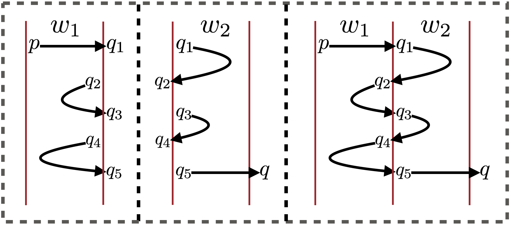
Figure 3: The first and second pictures are illustrations of subsets of $\mathsf{Tr}(w_{1})$ and $\mathsf{Tr}(w_{2})$ respectively. $(p,\rightarrow,q_{1}),(q_{2},\mathrel{\leavevmode\resizebox{1.5pt}{0.8pt}{\rotatebox[origin={c}]{90.0}{$\curvearrowleft$}}},q_{3}),(q_{4},\mathrel{\leavevmode\resizebox{1.5pt}{0.8pt}{\rotatebox[origin={c}]{90.0}{$\curvearrowleft$}}},q_{5})\in\mathsf{Tr}(w_{1})$ while $(q_{1},\mathrel{\leavevmode\resizebox{1.5pt}{0.8pt}{\rotatebox[origin={c}]{-90.0}{$\curvearrowright$}}},q_{2}),(q_{3},\mathrel{\leavevmode\resizebox{1.5pt}{0.8pt}{\rotatebox[origin={c}]{-90.0}{$\curvearrowright$}}},q_{4}),(q_{5},\rightarrow,q)\in\mathsf{Tr}(w_{2})$. The third picture shows that $(p,\rightarrow,q)\in\mathsf{Tr}(w_{1}\cdot w_{2})$: $(p,\rightarrow,q)$ consists of “steps” $(p,\rightarrow,q_{1}),(q_{1},\mathrel{\leavevmode\resizebox{1.5pt}{0.8pt}{\rotatebox[origin={c}]{-90.0}{$\curvearrowright$}}},q_{2}),(q_{2},\mathrel{\leavevmode\resizebox{1.5pt}{0.8pt}{\rotatebox[origin={c}]{90.0}{$\curvearrowleft$}}},q_{3}),(q_{3},\mathrel{\leavevmode\resizebox{1.5pt}{0.8pt}{\rotatebox[origin={c}]{-90.0}{$\curvearrowright$}}},q_{4}),(q_{4},\mathrel{\leavevmode\resizebox{1.5pt}{0.8pt}{\rotatebox[origin={c}]{90.0}{$\curvearrowleft$}}},q_{5}),(q_{5},\rightarrow,q)$ alternately from $\mathsf{Tr}(w_{1})$ and $\mathsf{Tr}(w_{2})$.

Example 2.10.

Let $\Sigma=\{a,b\}$ and let ${\mathcal{A}}$ be the following 1DFT:  .
Let $\mathsf{TrM}$ be the transition monoid of ${\mathcal{A}}$ and let $\mathsf{Tr}\colon\Sigma^{*}\to\mathsf{TrM}$ be the canonical morphism. The expression $F=a^{+}(ba)^{+}$ is not $\mathsf{Tr}$-good: one of the reasons why $F$ is not $\mathsf{Tr}$-good is that the subexpression $a^{+}$ is such that $\mathsf{Tr}(a)$ is not an idempotent; the same is true for the subexpression $(ba)^{+}$. The expression $F^{\prime}=aba\cup aaba\cup a(aa)^{+}ba\cup a(baba)^{+}\cup a(aa)^{+}(baba)^{+}$ is not $\mathsf{Tr}$-good, even though each of the expressions $aba,aaba,a(aa)^{+}ba,a(baba)^{+}$ and $a(aa)^{+}(baba)^{+}$ are $\mathsf{Tr}$-good. $F^{\prime}$ is not $\mathsf{Tr}$-good since $\mathsf{Tr}(\mathcal{L}(F^{\prime}))$ is not a singleton. The expression $F^{\prime\prime}=aba\cup(aa)^{+}\cup a(aa)^{+}ba$ is $\mathsf{Tr}$-good.

2.6 2DFT to RTE

Consider a deterministic and complete 2-way transducer $\mathcal{A}$. Let $\mathsf{TrM}$ be the transition monoid of the underlying input automaton. We can apply the unambiguous factorization theorem to the morphism $\mathsf{Tr}\colon\Sigma^{*}\to\mathsf{TrM}$ in order to obtain, for each $s\in\mathsf{TrM}$, an $\varepsilon$-free good rational expression $F_{s}$ for $\mathsf{Tr}^{-1}(s)\setminus\{\varepsilon\}$. We use the unambiguous expression $G=\varepsilon\cup\bigcup_{s\in\mathsf{TrM}}F_{s}$ as a guide when constructing RTEs corresponding to the 2DFT $\mathcal{A}$.

Lemma 2.11.

Let $F$ be an $\varepsilon$-free $\mathsf{Tr}$-good rational expression and let $\mathsf{Tr}(F)=s_{F}$ be the corresponding element of the transition monoid $\mathsf{TrM}$ of $\mathcal{A}$. We can construct a map $C_{F}\colon s_{F}\to\textsf{RTE}$ such that for each step $x=(p,d,q)\in s_{F}$ the following invariants hold:

1. $\mathsf{dom}(C_{F}(x))=\mathcal{L}(F)$,

2. for each $u\in\mathcal{L}(F)$, $[\![C_{F}(x)]\!](u)$ is the output produced by $\mathcal{A}$ when running step $x$ on $u$ (i.e., running $\mathcal{A}$ on $u$ from $p$ to $q$ following direction $d$).

Proof 2.12.

The proof is by structural induction on the rational expression. For each subexpression $E$ of $F$ we let $\mathsf{Tr}(E)=s_{E}$ be the corresponding element of the transition monoid $\mathsf{TrM}$ of $\mathcal{A}$. We start with atomic regular expressions. Since $F$ is $\varepsilon$-free and $\emptyset$-free, we do not need to consider $E=\varepsilon$ or $E=\emptyset$.

atomic

Assume that $E=a\in\Sigma$ is an atomic subexpression. Since the 2DFT $\mathcal{A}$ is deterministic and complete, for each state $p\in Q$ we have

• either $\delta(p,a)=(q,\gamma,1)$ and we let $C_{a}((p,\rightarrow,q))=C_{a}((p,\mathrel{\leavevmode\resizebox{1.5pt}{0.8pt}{\rotatebox[origin={c}]{90.0}{$\curvearrowleft$}}},q))={a}\,?\,{\gamma}:{\bot}$,

• or $\delta(p,a)=(q,\gamma,-1)$ and we let $C_{a}((p,\mathrel{\leavevmode\resizebox{1.5pt}{0.8pt}{\rotatebox[origin={c}]{-90.0}{$\curvearrowright$}}},q))=C_{a}((p,\leftarrow,q))={a}\,?\,{\gamma}:{\bot}$.

Clearly, invariants ($\mathsf{I}_{1}$) and ($\mathsf{I}_{2}$) hold for all $x\in\mathsf{Tr}(a)=s_{E}$.

Union

Assume that $E=E_{1}\cup E_{2}$. Since the expression is good, we deduce that $s_{E}=s_{E_{1}}=s_{E_{2}}$. For each $x\in s_{E}$ we define $C_{E}(x)={E_{1}}\,?\,{C_{E_{1}}(x)}:{C_{E_{2}}(x)}$. Since $E$ is unambiguous we have $\mathcal{L}(E_{1})\cap\mathcal{L}(E_{2})=\emptyset$. Using ($\mathsf{I}_{1}$) for $E_{1}$ and $E_{2}$, we deduce that

$$\mathsf{dom}(C_{E}(x)) =(\mathcal{L}(E_{1})\cap\mathsf{dom}(C_{E_{1}}(x)))\cup(\mathsf{dom}(C_{E_{2}}(x))\setminus\mathcal{L}(E_{1}))=\mathcal{L}(E_{1})\cup\mathcal{L}(E_{2})=\mathcal{L}(E)\,.$$

Therefore, ($\mathsf{I}_{1}$) holds for $E$. Now, for each $u\in\mathcal{L}(E)$, either $u\in\mathcal{L}(E_{1})$ and $[\![C_{E}(x)]\!](u)=[\![C_{E_{1}}(x)]\!](u)$ or $u\in\mathcal{L}(E_{2})$ and $[\![C_{E}(x)]\!](u)=[\![C_{E_{2}}(x)]\!](u)$. In both cases, applying ($\mathsf{I}_{2}$) for $E_{1}$ or $E_{2}$, we deduce that $[\![C_{E}(x)]\!](u)$ is the output produced by $\mathcal{A}$ when running step $x$ on $u$.

concatenation

Assume that $E=E_{1}\cdot E_{2}$ is a concatenation. Since the expression is good, we deduce that $s_{E}=s_{E_{1}}\cdot s_{E_{2}}$. Let $x\in s_{E}$.

• If $x=(p,\rightarrow,q)$ then, by definition of the product in the transition monoid $\mathsf{TrM}$, there is a unique sequence of steps $x_{1}=(p,\rightarrow,q_{1})$, $x_{2}=(q_{1},\mathrel{\leavevmode\resizebox{1.5pt}{0.8pt}{\rotatebox[origin={c}]{-90.0}{$\curvearrowright$}}},q_{2})$, $x_{3}=(q_{2},\mathrel{\leavevmode\resizebox{1.5pt}{0.8pt}{\rotatebox[origin={c}]{90.0}{$\curvearrowleft$}}},q_{3})$, $x_{4}=(q_{3},\mathrel{\leavevmode\resizebox{1.5pt}{0.8pt}{\rotatebox[origin={c}]{-90.0}{$\curvearrowright$}}},q_{4})$, …, $x_{i}=(q_{i-1},\mathrel{\leavevmode\resizebox{1.5pt}{0.8pt}{\rotatebox[origin={c}]{90.0}{$\curvearrowleft$}}},q_{i})$, $x_{i+1}=(q_{i},\rightarrow,q)$ with $i\geq 1$, $x_{1},x_{3},\ldots,x_{i}\in s_{E_{1}}$ and $x_{2},x_{4},\ldots,x_{i+1}\in s_{E_{2}}$ (see Figure 3). We define

  $$C_{E}(x)=(C_{E_{1}}(x_{1})\mathbin{{\boxdot}}C_{E_{2}}(x_{2}))\odot(C_{E_{1}}(x_{3})\mathbin{{\boxdot}}C_{E_{2}}(x_{4}))\odot\cdots\odot(C_{E_{1}}(x_{i})\mathbin{{\boxdot}}C_{E_{2}}(x_{i+1}))\,.$$

  Notice that when $i=1$ we simply have $C_{E}(x)=C_{E_{1}}(x_{1})\mathbin{{\boxdot}}C_{E_{2}}(x_{2})$ with $x_{2}=(q_{1},\rightarrow,q)$.

  The concatenation $\mathcal{L}(E)=\mathcal{L}(E_{1})\cdot\mathcal{L}(E_{2})$ is unambiguous. Therefore, for all $y\in s_{E_{1}}$ and $z\in s_{E_{2}}$, using ($\mathsf{I}_{1}$) for $E_{1}$ and $E_{2}$, we obtain $\mathsf{dom}(C_{E_{1}}(y)\mathbin{{\boxdot}}C_{E_{2}}(z))=\mathcal{L}(E)$. We deduce that $\mathsf{dom}(C_{E}(x))=\mathcal{L}(E)$ and ($\mathsf{I}_{1}$) holds for $E$.

  Now, let $u\in\mathcal{L}(E)$ and let $u=u_{1}u_{2}$ be its unique factorization with $u_{1}\in\mathcal{L}(E_{1})$ and $u_{2}\in\mathcal{L}(E_{2})$. The step $x=(p,\rightarrow,q)$ performed by $\mathcal{A}$ on $u$ is actually the concatenation of steps $x_{1}$ on $u_{1}$, followed by $x_{2}$ on $u_{2}$, followed by $x_{3}$ on $u_{1}$, followed by $x_{4}$ on $u_{2}$, …, until $x_{i+1}$ on $u_{2}$. Using ($\mathsf{I}_{2}$) for $E_{1}$ and $E_{2}$, we deduce that the output produced by $\mathcal{A}$ while running step $x$ on $u$ is

  $$[\![C_{E_{1}}(x_{1})]\!](u_{1})\cdot[\![C_{E_{2}}(x_{2})]\!](u_{2})\cdots[\![C_{E_{1}}(x_{i})]\!](u_{1})\cdot[\![C_{E_{2}}(x_{i+1})]\!](u_{2})=[\![C_{E}(x)]\!](u)\,.$$

• If $x=(p,\mathrel{\leavevmode\resizebox{1.5pt}{0.8pt}{\rotatebox[origin={c}]{-90.0}{$\curvearrowright$}}},q)$ then, following the definition of the product in the transition monoid $\mathsf{TrM}$, we distinguish two cases.

  Either $x\in s_{E_{1}}$ and we let $C_{E}(x)=C_{E_{1}}(x)\mathbin{{\boxdot}}({E_{2}}\,?\,{\varepsilon}:{\bot})$. Since $\mathsf{dom}({E_{2}}\,?\,{\varepsilon}:{\bot})=\mathcal{L}(E_{2})$, we deduce as above that $\mathsf{dom}(C_{E}(x))=\mathcal{L}(E)$. Moreover, let $u\in\mathcal{L}(E)$ and $u=u_{1}u_{2}$ be its unique factorization with $u_{1}\in\mathcal{L}(E_{1})$ and $u_{2}\in\mathcal{L}(E_{2})$. The step $x=(p,\mathrel{\leavevmode\resizebox{1.5pt}{0.8pt}{\rotatebox[origin={c}]{-90.0}{$\curvearrowright$}}},q)$ performed by $\mathcal{A}$ on $u$ reduces to the step $x$ on $u_{1}$. Using ($\mathsf{I}_{2}$) for $E_{1}$, we deduce that the output produced by $\mathcal{A}$ while making step $x$ on $u$ is $[\![C_{E_{1}}(x)]\!](u_{1})=[\![C_{E}(x)]\!](u)$.

  

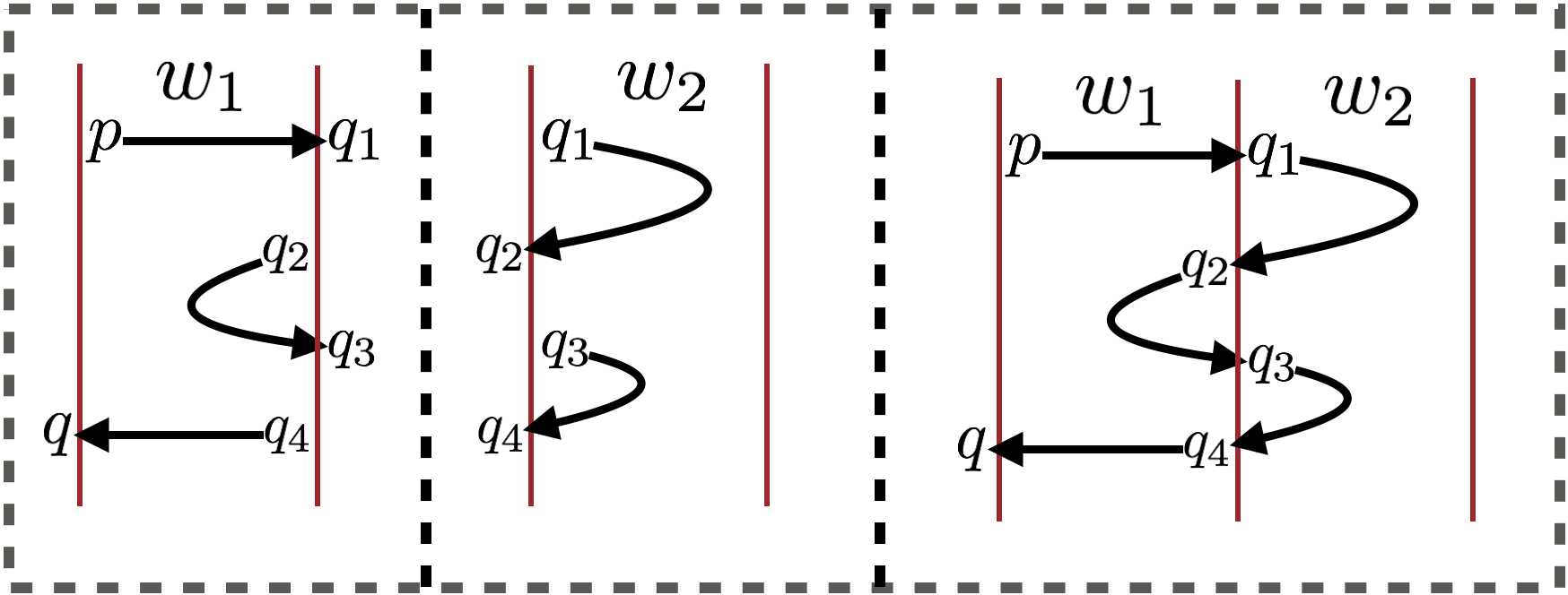
  Figure 4: Let $w=w_{1}\cdot w_{2}\in\mathcal{L}(E)$ with $w_{1}\in\mathcal{L}(E_{1})$, $w_{2}\in\mathcal{L}(E_{2})$. We have $(p,\rightarrow,q_{1}),(q_{2},\mathrel{\leavevmode\resizebox{1.5pt}{0.8pt}{\rotatebox[origin={c}]{90.0}{$\curvearrowleft$}}},q_{3}),(q_{4},\leftarrow,q)\in\mathsf{Tr}(w_{1})$ and $(q_{1},\mathrel{\leavevmode\resizebox{1.5pt}{0.8pt}{\rotatebox[origin={c}]{-90.0}{$\curvearrowright$}}},q_{2}),(q_{3},\mathrel{\leavevmode\resizebox{1.5pt}{0.8pt}{\rotatebox[origin={c}]{-90.0}{$\curvearrowright$}}},q_{4})\in\mathsf{Tr}(w_{2})$. Then $(p,\mathrel{\leavevmode\resizebox{1.5pt}{0.8pt}{\rotatebox[origin={c}]{-90.0}{$\curvearrowright$}}},q)$ is composed of “steps” $(p,\rightarrow,q_{1}),(q_{1},\mathrel{\leavevmode\resizebox{1.5pt}{0.8pt}{\rotatebox[origin={c}]{-90.0}{$\curvearrowright$}}},q_{2}),(q_{2},\mathrel{\leavevmode\resizebox{1.5pt}{0.8pt}{\rotatebox[origin={c}]{90.0}{$\curvearrowleft$}}},q_{3}),(q_{3},\mathrel{\leavevmode\resizebox{1.5pt}{0.8pt}{\rotatebox[origin={c}]{-90.0}{$\curvearrowright$}}},q_{4}),(q_{4},\leftarrow,q)$ alternately from $\mathsf{Tr}(w_{1})$ and $\mathsf{Tr}(w_{2})$.

  Or there is a unique sequence of steps (see Figure 4) $x_{1}=(p,\rightarrow,q_{1})$, $x_{2}=(q_{1},\mathrel{\leavevmode\resizebox{1.5pt}{0.8pt}{\rotatebox[origin={c}]{-90.0}{$\curvearrowright$}}},q_{2})$, $x_{3}=(q_{2},\mathrel{\leavevmode\resizebox{1.5pt}{0.8pt}{\rotatebox[origin={c}]{90.0}{$\curvearrowleft$}}},q_{3})$, $x_{4}=(q_{3},\mathrel{\leavevmode\resizebox{1.5pt}{0.8pt}{\rotatebox[origin={c}]{-90.0}{$\curvearrowright$}}},q_{4})$, …, $x_{i}=(q_{i-1},\leftarrow,q)$ with $i\geq 3$, $x_{1},x_{3},\ldots,x_{i}\in s_{E_{1}}$ and $x_{2},x_{4},\ldots,x_{i-1}\in s_{E_{2}}$. We define

  $$C_{E}(x)=(C_{E_{1}}(x_{1})\mathbin{{\boxdot}}C_{E_{2}}(x_{2}))\odot(C_{E_{1}}(x_{3})\mathbin{{\boxdot}}C_{E_{2}}(x_{4}))\odot\cdots\odot(C_{E_{1}}(x_{i})\mathbin{{\boxdot}}({E_{2}}\,?\,{\varepsilon}:{\bot}))\,.$$

  As for the first item, we can prove that invariants ($\mathsf{I}_{1}$) and ($\mathsf{I}_{2}$) are satisfied for $E$.

• The cases $x=(p,\leftarrow,q)$ or $x=(p,\mathrel{\leavevmode\resizebox{1.5pt}{0.8pt}{\rotatebox[origin={c}]{90.0}{$\curvearrowleft$}}},q)$ are handled symmetrically. For instance, when $x=(p,\leftarrow,q)$, the unique sequence of steps is $x_{1}=(p,\leftarrow,q_{1})$, $x_{2}=(q_{1},\mathrel{\leavevmode\resizebox{1.5pt}{0.8pt}{\rotatebox[origin={c}]{90.0}{$\curvearrowleft$}}},q_{2})$, $x_{3}=(q_{2},\mathrel{\leavevmode\resizebox{1.5pt}{0.8pt}{\rotatebox[origin={c}]{-90.0}{$\curvearrowright$}}},q_{3})$, $x_{4}=(q_{3},\mathrel{\leavevmode\resizebox{1.5pt}{0.8pt}{\rotatebox[origin={c}]{90.0}{$\curvearrowleft$}}},q_{4})$, …, $x_{i}=(q_{i-1},\mathrel{\leavevmode\resizebox{1.5pt}{0.8pt}{\rotatebox[origin={c}]{-90.0}{$\curvearrowright$}}},q_{i})$, $x_{i+1}=(q_{i},\leftarrow,q)$ with $i\geq 1$, $x_{1},x_{3},\ldots,x_{i}\in s_{E_{2}}$ and $x_{2},x_{4},\ldots,x_{i+1}\in s_{E_{1}}$ (see Figure 5). We define

  $$C_{E}(x)=(({E_{1}}\,?\,{\varepsilon}:{\bot})\mathbin{{\boxdot}}C_{E_{2}}(x_{1})) \odot(C_{E_{1}}(x_{2})\mathbin{{\boxdot}}C_{E_{2}}(x_{3}))\odot\cdots\odot{}$$

  $$(C_{E_{1}}(x_{i-1})\mathbin{{\boxdot}}C_{E_{2}}(x_{i})) \odot(C_{E_{1}}(x_{i+1})\mathbin{{\boxdot}}({E_{2}}\,?\,{\varepsilon}:{\bot}))\,.$$

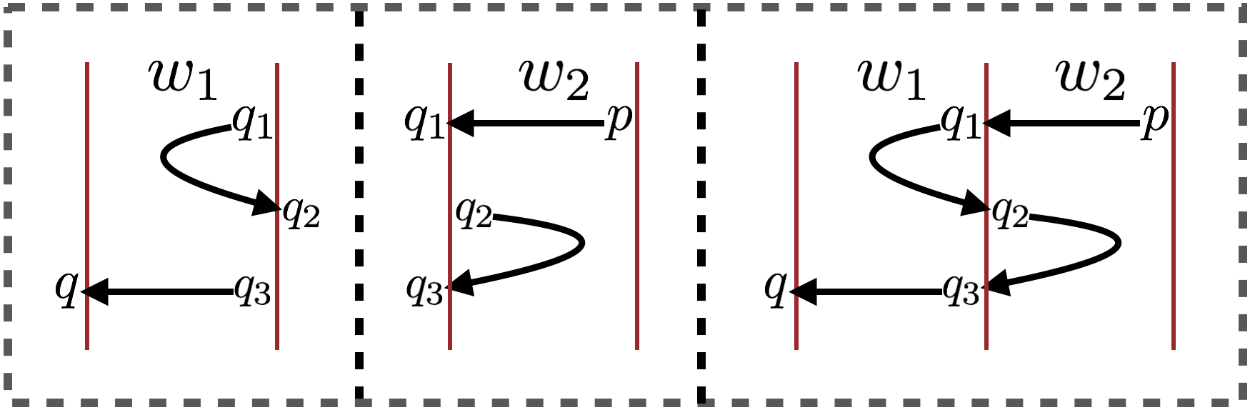
Figure 5: Let $w=w_{1}\cdot w_{2}\in\mathcal{L}(E)$ with $w_{1}\in\mathcal{L}(E_{1})$, $w_{2}\in\mathcal{L}(E_{2})$. We have $(p,\leftarrow,q_{1}),(q_{2},\mathrel{\leavevmode\resizebox{1.5pt}{0.8pt}{\rotatebox[origin={c}]{-90.0}{$\curvearrowright$}}},q_{3})\in\mathsf{Tr}(w_{2})$ and $(q_{1},\mathrel{\leavevmode\resizebox{1.5pt}{0.8pt}{\rotatebox[origin={c}]{90.0}{$\curvearrowleft$}}},q_{2}),(q_{3},\leftarrow,q)\in\mathsf{Tr}(w_{1})$. Then $(p,\leftarrow,q)\in\mathsf{Tr}(w)$ is composed of “steps” $(p,\leftarrow,q_{1}),(q_{1},\mathrel{\leavevmode\resizebox{1.5pt}{0.8pt}{\rotatebox[origin={c}]{90.0}{$\curvearrowleft$}}},q_{2}),(q_{2},\mathrel{\leavevmode\resizebox{1.5pt}{0.8pt}{\rotatebox[origin={c}]{-90.0}{$\curvearrowright$}}},q_{3}),(q_{3},\leftarrow,q)$ alternately from $\mathsf{Tr}(w_{2})$ and $\mathsf{Tr}(w_{1})$.

Kleene-plus

Assume that $E=F^{+}$. Since the expression is good, we deduce that $s_{E}=s_{F}=s$ is an idempotent of the transition monoid $\mathsf{TrM}$. Let $x\in s$.

• If $x=(p,\mathrel{\leavevmode\resizebox{1.5pt}{0.8pt}{\rotatebox[origin={c}]{-90.0}{$\curvearrowright$}}},q)$. Since $F^{+}$ is unambiguous, a word $u\in\mathcal{L}(F^{+})$ admits a unique factorization $u=u_{1}u_{2}\cdots u_{n}$ with $n\geq 1$ and $u_{i}\in\mathcal{L}(F)$. Now, $\mathsf{Tr}(u_{1})=s_{E}$ and since $x=(p,\mathrel{\leavevmode\resizebox{1.5pt}{0.8pt}{\rotatebox[origin={c}]{-90.0}{$\curvearrowright$}}},q)\in s_{E}$ the unique run $\rho$ of $\mathcal{A}$ starting in state $p$ on the left of $u_{1}$ exits on the left in state $q$. Therefore, the unique run of $\mathcal{A}$ starting in state $p$ on the left of $u=u_{1}u_{2}\cdots u_{n}$ only visits $u_{1}$ and is actually $\rho$ itself. Therefore, we set $C_{E}(x)=C_{F}(x)\mathbin{{\boxdot}}({F^{*}}\,?\,{\varepsilon}:{\bot})$ and we can easily check that ($\mathsf{I}_{1}$–$\mathsf{I}_{2}$) are satisfied.

• Similarly for $x=(p,\mathrel{\leavevmode\resizebox{1.5pt}{0.8pt}{\rotatebox[origin={c}]{90.0}{$\curvearrowleft$}}},q)$ we set $C_{E}(x)=({F^{*}}\,?\,{\varepsilon}:{\bot})\mathbin{{\boxdot}}C_{F}(x)$.

• If $x=(p,\rightarrow,q)$. Recall that $s$ is an idempotent, hence $x\in s^{2}$. We distinguish two cases.

  Either $y=(q,\rightarrow,q)\in s$ and we set $C_{E}(x)={F}\,?\,{C_{F}(x)}:{\big{(}C_{F}(x)\mathbin{{\boxdot}}{(C_{F}(y))}^{\scriptstyle{\boxplus}}\big{)}}$.

  

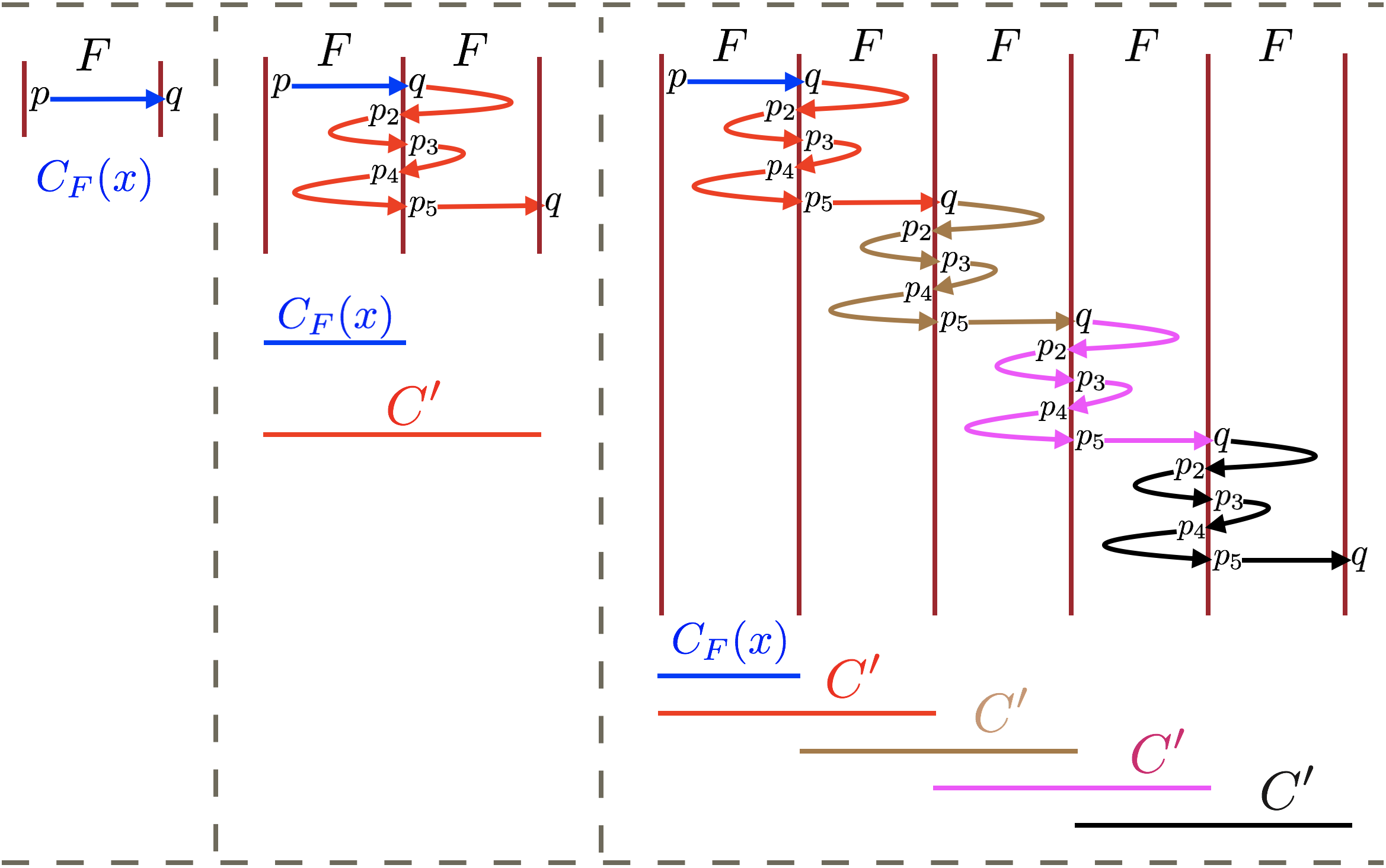
  Figure 6: In the Kleene-plus $E=F^{+}$, a step $x=(p,\rightarrow,q)\in s_{E}$ on some $u=u_{1}u_{2}\cdots u_{n}$ with $u_{\ell}\in\mathcal{L}(F)$ is obtained by composing the following steps in $s_{F}$: $x_{1}=x$, $x_{2}=(q,\mathrel{\leavevmode\resizebox{1.5pt}{0.8pt}{\rotatebox[origin={c}]{-90.0}{$\curvearrowright$}}},p_{2})$, $x_{3}=(p_{2},\mathrel{\leavevmode\resizebox{1.5pt}{0.8pt}{\rotatebox[origin={c}]{90.0}{$\curvearrowleft$}}},p_{3})$, $x_{4}=(p_{3},\mathrel{\leavevmode\resizebox{1.5pt}{0.8pt}{\rotatebox[origin={c}]{-90.0}{$\curvearrowright$}}},p_{4})$, $x_{5}=(p_{4},\mathrel{\leavevmode\resizebox{1.5pt}{0.8pt}{\rotatebox[origin={c}]{90.0}{$\curvearrowleft$}}},p_{5})$, $x_{6}=(p_{5},\rightarrow,q)$.

  Or there exists a unique sequence of steps in $s$: $x_{1}=x$, $x_{2}=(q,\mathrel{\leavevmode\resizebox{1.5pt}{0.8pt}{\rotatebox[origin={c}]{-90.0}{$\curvearrowright$}}},p_{2})$, $x_{3}=(p_{2},\mathrel{\leavevmode\resizebox{1.5pt}{0.8pt}{\rotatebox[origin={c}]{90.0}{$\curvearrowleft$}}},p_{3})$, $x_{4}=(p_{3},\mathrel{\leavevmode\resizebox{1.5pt}{0.8pt}{\rotatebox[origin={c}]{-90.0}{$\curvearrowright$}}},p_{4})$, …, $x_{i}=(p_{i-1},\mathrel{\leavevmode\resizebox{1.5pt}{0.8pt}{\rotatebox[origin={c}]{90.0}{$\curvearrowleft$}}},p_{i})$, $x_{i+1}=(p_{i},\rightarrow,q)$ with $i\geq 3$ (see Figure 6). We define

  $$C_{E}(x) =\big{(}C_{F}(x)\mathbin{{\boxdot}}({F^{*}}\,?\,{\varepsilon}:{\bot})\big{)}\odot[F,C^{\prime}]^{2\scriptstyle{\boxplus}}$$

  $$C^{\prime} =\big{(}({F}\,?\,{\varepsilon}:{\bot})\mathbin{{\boxdot}}C_{F}(x_{2})\big{)}\odot(C_{F}(x_{3})\mathbin{{\boxdot}}C_{F}(x_{4}))\odot\cdots\odot(C_{F}(x_{i})\mathbin{{\boxdot}}C_{F}(x_{i+1}))$$

  Since the expression is good, the Kleene-plus $E=F^{+}$ is unambiguous. We have $\mathsf{dom}(C_{F}(x_{j}))=\mathcal{L}(F)$ for $1\leq j\leq i+1$ by ($\mathsf{I}_{1}$). Also $\mathsf{dom}({F^{*}}\,?\,{\varepsilon}:{\bot})=\mathcal{L}(F^{*})$. Since $F^{+}$ is unambiguous, the concatenation $F\cdot F^{*}$ is also unambiguous and we get $\mathsf{dom}(C_{F}(x)\mathbin{{\boxdot}}({F^{*}}\,?\,{\varepsilon}:{\bot}))=\mathcal{L}(F)\cdot\mathcal{L}(F^{*})=\mathcal{L}(E)$. Also, the product $F\cdot F$ is unambiguous and we deduce that $\mathsf{dom}(C_{F}(x_{j})\mathbin{{\boxdot}}C_{F}(x_{j+1}))=\mathcal{L}(F)^{2}$ for $1\leq j\leq i$ and $\mathsf{dom}(({F}\,?\,{\varepsilon}:{\bot})\mathbin{{\boxdot}}C_{F}(x_{2}))=\mathcal{L}(F)^{2}$. Therefore, $\mathsf{dom}(C^{\prime})=\mathcal{L}(F)^{2}$ and using once again that $F^{+}$ is unambiguous, we deduce that $\mathsf{dom}([F,C^{\prime}]^{2\scriptstyle{\boxplus}})=\mathcal{L}(F^{+})=\mathcal{L}(E)$. We deduce that $\mathsf{dom}(C_{E}(x))=\mathcal{L}(E)$ and ($\mathsf{I}_{1}$) holds for $E$.

  Let now $u\in\mathcal{L}(F^{+})=\mathsf{dom}(C_{E}(x))$. We have to show that the output $\gamma\in\mathbb{D}$ produced by $\mathcal{A}$ when running step $x$ on $u$ is $[\![C_{E}(x)]\!](u)$. There is a unique factorization $u=u_{1}u_{2}\cdots u_{n}$ with $n\geq 1$ and $u_{\ell}\in\mathcal{L}(F)$ for $1\leq\ell\leq n$.

  Assume first that $n=1$ (see Figure 6 left). By definition, we have $[\![[F,C^{\prime}]^{2\scriptstyle{\boxplus}}]\!](u)=\varepsilon$ and $[\![C_{F}(x)\mathbin{{\boxdot}}({F^{*}}\,?\,{\varepsilon}:{\bot})]\!](u)=[\![C_{F}(x)]\!](u)$ which, by induction, is the output $\gamma$ produced by $\mathcal{A}$ running step $x$ on $u$. Therefore, $[\![C_{E}(x)]\!](u)=\gamma\cdot\varepsilon=\gamma$.

  Assume now that $n\geq 2$ (see Figure 6 middle for $n=2$ and right for $n=5$). For $1\leq\ell\leq n$ and $1\leq j\leq i+1$, we denote $\gamma^{\ell}_{j}=[\![C_{F}(x_{j})]\!](u_{\ell})$ the output produced by $\mathcal{A}$ when running step $x_{j}$ on $u_{\ell}$. We can check (see Figure 6) that the output $\gamma$ produced by $\mathcal{A}$ when running $x$ on $u=u_{1}u_{2}\cdots u_{n}$ is

  $$\gamma=\gamma_{1}^{1}(\gamma_{2}^{2}\gamma_{3}^{1}\gamma_{4}^{2}\cdots\gamma_{i}^{1}\gamma_{i+1}^{2})(\gamma_{2}^{3}\gamma_{3}^{2}\gamma_{4}^{3}\cdots\gamma_{i}^{2}\gamma_{i+1}^{3})\cdots(\gamma_{2}^{n}\gamma_{3}^{n-1}\gamma_{4}^{n}\cdots\gamma_{i}^{n-1}\gamma_{i+1}^{n})\,.$$

  We have $[\![C^{\prime}]\!](u_{\ell}u_{\ell+1})=\gamma_{2}^{\ell+1}\gamma_{3}^{\ell}\gamma_{4}^{\ell+1}\cdots\gamma_{i}^{\ell}\gamma_{i+1}^{\ell+1}$ for $1\leq\ell<n$. Therefore, we obtain $\gamma=\gamma_{1}^{1}[\![C^{\prime}]\!](u_{1}u_{2})[\![C^{\prime}]\!](u_{2}u_{3})\cdots[\![C^{\prime}]\!](u_{n-1}u_{n})$. Since $[\![C_{F}(x)\mathbin{{\boxdot}}({F^{*}}\,?\,{\varepsilon}:{\bot})]\!](u)=\gamma_{1}^{1}$ we deduce that $\gamma=[\![C_{E}(x)]\!](u)$.

• The case of $x=(p,\leftarrow,q)$ can be handled similarly.

Lemma 2.11 is the main ingredient in the construction of an RTE equivalent to a 2DFT.

Proof 2.13 (Proof of Theorem 2.6(2)).

First, we let $C_{\varepsilon}=[\![\mathcal{A}]\!](\varepsilon)\in\Gamma^{*}\cup\{\bot\}$. Then, we will define for each $s\in\mathsf{TrM}$, an RTE $C_{s}$ such that $\mathsf{dom}(C_{s})=\mathsf{dom}(\mathcal{A})\cap(\mathsf{Tr}^{-1}(s)\setminus\{\varepsilon\})$ and $[\![C_{s}]\!](u)=[\![\mathcal{A}]\!](u)$ for all $u\in\mathsf{dom}(C_{s})$. Assuming an arbitrary enumeration $s_{1},s_{2},\ldots,s_{m}$ of $\mathsf{TrM}$, we define the final RTE as

$$C_{\mathcal{A}}={\varepsilon}\,?\,{C_{\varepsilon}}:{({\mathsf{Tr}^{-1}(s_{1})}\,?\,{C_{s_{1}}}:{({\mathsf{Tr}^{-1}(s_{2})}\,?\,{C_{s_{2}}}:{\cdots({\mathsf{Tr}^{-1}(s_{m-1})}\,?\,{C_{s_{m-1}}}:{C_{s_{m}}})})})}\,.$$

It remains to define the RTE $C_{s}$ for $s\in\mathsf{TrM}$. We first define RTEs for steps in the 2DFT $\mathcal{A}$ on some input ${\vdash}u$ with $u\in\mathsf{Tr}^{-1}(s)\setminus\{\varepsilon\}$. Such a step must exit on the right since there are no transitions of $\mathcal{A}$ going left when reading ${\vdash}$. So either the step $(q_{0},\rightarrow,q)$ starts on the left in the initial state $q_{0}$ and exits on the right in some state $q$. Or the step $(p,\mathrel{\leavevmode\resizebox{1.5pt}{0.8pt}{\rotatebox[origin={c}]{90.0}{$\curvearrowleft$}}},q)$ starts on the right in state $p$ and exits on the right in state $q$. See Figure 7.

Let $s_{\vdash}$ be the set of steps $(p,\rightarrow,q),(p,\mathrel{\leavevmode\resizebox{1.5pt}{0.8pt}{\rotatebox[origin={c}]{90.0}{$\curvearrowleft$}}},q)$ such that there is a transition $\delta(p,{\vdash})=(q,\gamma_{p},+1)$ in $\mathcal{A}$. From the initial state $q_{0}$ of $\mathcal{A}$, there is a unique sequence of steps $x_{1}=(q_{0},\rightarrow,q_{1})$, $x_{2}=(q_{1},\mathrel{\leavevmode\resizebox{1.5pt}{0.8pt}{\rotatebox[origin={c}]{-90.0}{$\curvearrowright$}}},q_{2})$, $x_{3}=(q_{2},\mathrel{\leavevmode\resizebox{1.5pt}{0.8pt}{\rotatebox[origin={c}]{90.0}{$\curvearrowleft$}}},q_{3})$, $x_{4}=(q_{3},\mathrel{\leavevmode\resizebox{1.5pt}{0.8pt}{\rotatebox[origin={c}]{-90.0}{$\curvearrowright$}}},q_{4})$, …, $x_{i}=(q_{i-1},\mathrel{\leavevmode\resizebox{1.5pt}{0.8pt}{\rotatebox[origin={c}]{90.0}{$\curvearrowleft$}}},q_{i})$, $x_{i+1}=(q_{i},\rightarrow,q)$ with $i\geq 1$, $x_{1},x_{3},\ldots,x_{i}\in s_{\vdash}$ and $x_{2},x_{4},\ldots,x_{i+1}\in s$ (see Figure 7 left). We define

$$C_{{\vdash}F_{s}}((q_{0},\rightarrow,q))=\gamma_{q_{0}}\odot C_{F_{s}}(x_{2})\odot\gamma_{q_{2}}\odot C_{F_{s}}(x_{4})\odot\cdots\odot\gamma_{q_{i-1}}\odot C_{F_{s}}(x_{i+1})\,.$$

Notice that when $i=1$ we simply have $C_{{\vdash}F_{s}}((q_{0},\rightarrow,q))=\gamma_{q_{0}}\odot C_{F_{s}}((q_{1},\rightarrow,q))$. Since $\mathsf{dom}(C_{F_{s}}(x_{i}))=\mathcal{L}(F_{s})=\mathsf{Tr}^{-1}(s)\setminus\{\varepsilon\}$ for $i=2,4,\ldots,i+1$, we deduce that $\mathsf{dom}(C_{{\vdash}F_{s}}((q_{0},\rightarrow,q)))=\mathsf{Tr}^{-1}(s)\setminus\{\varepsilon\}$. Moreover, for each $u\in\mathsf{Tr}^{-1}(s)\setminus\{\varepsilon\}$, the output produced by $\mathcal{A}$ performing step $(q_{0},\rightarrow,q)$ on ${\vdash}u$ is $[\![C_{{\vdash}F_{s}}((q_{0},\rightarrow,q))]\!](u)$.

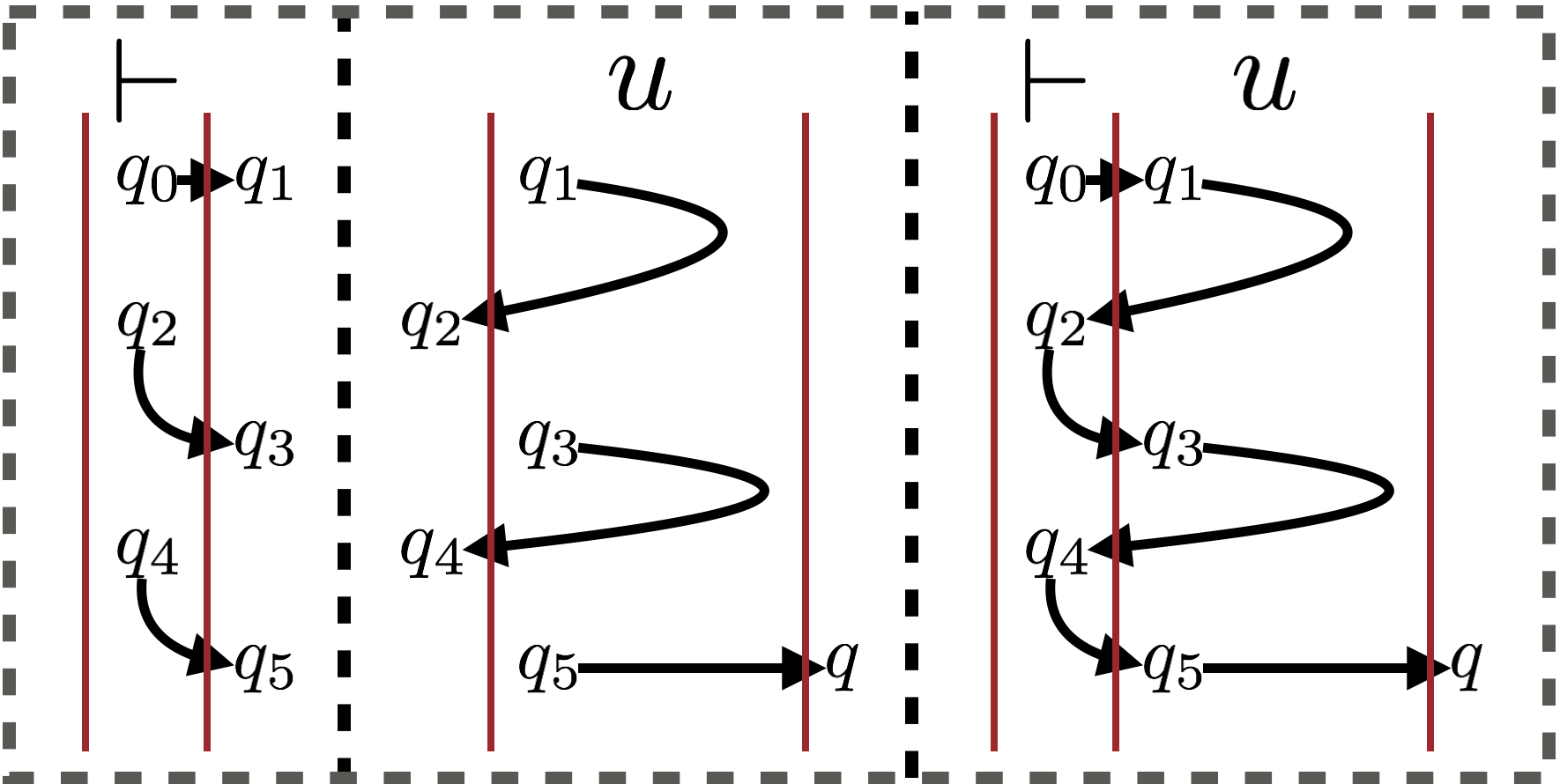
Figure 7:

Let $p$ be a state of $\mathcal{A}$. Either there is a step $(p,\mathrel{\leavevmode\resizebox{1.5pt}{0.8pt}{\rotatebox[origin={c}]{90.0}{$\curvearrowleft$}}},q)\in s$ and we let $C_{{\vdash}F_{s}}((p,\mathrel{\leavevmode\resizebox{1.5pt}{0.8pt}{\rotatebox[origin={c}]{90.0}{$\curvearrowleft$}}},q))=C_{F_{s}}((p,\mathrel{\leavevmode\resizebox{1.5pt}{0.8pt}{\rotatebox[origin={c}]{90.0}{$\curvearrowleft$}}},q))$. Or, there is a unique sequence of steps $x_{1}=(p,\leftarrow,q_{1})$, $x_{2}=(q_{1},\mathrel{\leavevmode\resizebox{1.5pt}{0.8pt}{\rotatebox[origin={c}]{90.0}{$\curvearrowleft$}}},q_{2})$, $x_{3}=(q_{2},\mathrel{\leavevmode\resizebox{1.5pt}{0.8pt}{\rotatebox[origin={c}]{-90.0}{$\curvearrowright$}}},q_{3})$, $x_{4}=(q_{3},\mathrel{\leavevmode\resizebox{1.5pt}{0.8pt}{\rotatebox[origin={c}]{90.0}{$\curvearrowleft$}}},q_{4})$, …, $x_{i}=(q_{i-1},\rightarrow,q)$ with $i\geq 3$, $x_{1},x_{3},\ldots,x_{i}\in s$ and $x_{2},x_{4},\ldots,x_{i-1}\in s_{\vdash}$ (see Figure 7 right). We define

$$C_{{\vdash}F_{s}}((p,\mathrel{\leavevmode\resizebox{1.5pt}{0.8pt}{\rotatebox[origin={c}]{90.0}{$\curvearrowleft$}}},q))=C_{F_{s}}(x_{1})\odot\gamma_{q_{1}}\odot C_{F_{s}}(x_{3})\odot\gamma_{q_{3}}\odot\cdots\odot\gamma_{q_{i-2}}\odot C_{F_{s}}(x_{i})\,.$$

As above, we have $\mathsf{dom}(C_{{\vdash}F_{s}}((p,\mathrel{\leavevmode\resizebox{1.5pt}{0.8pt}{\rotatebox[origin={c}]{90.0}{$\curvearrowleft$}}},q)))=\mathsf{Tr}^{-1}(s)\setminus\{\varepsilon\}$. Moreover, for each $u\in\mathsf{Tr}^{-1}(s)\setminus\{\varepsilon\}$, the output produced by $\mathcal{A}$ performing step $(p,\mathrel{\leavevmode\resizebox{1.5pt}{0.8pt}{\rotatebox[origin={c}]{90.0}{$\curvearrowleft$}}},q)$ on ${\vdash}u$ is $[\![C_{{\vdash}F_{s}}((p,\mathrel{\leavevmode\resizebox{1.5pt}{0.8pt}{\rotatebox[origin={c}]{90.0}{$\curvearrowleft$}}},q))]\!](u)$.

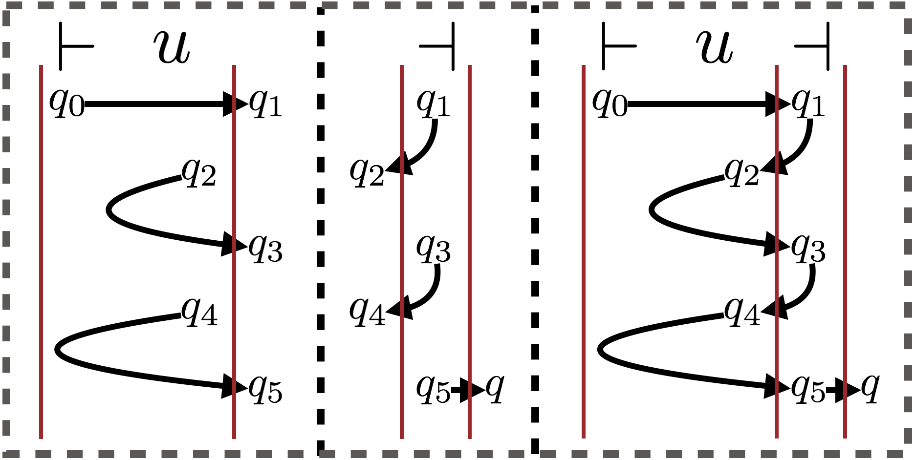
Figure 8:

Similarly, let $s_{\dashv}$ be the set of steps $(p,\mathrel{\leavevmode\resizebox{1.5pt}{0.8pt}{\rotatebox[origin={c}]{-90.0}{$\curvearrowright$}}},q)$ such that there is a transition $\delta(p,{\dashv})=(q,\gamma_{p},-1)$ in $\mathcal{A}$ or $(p,\rightarrow,q)$ such that there is a transition $\delta(p,{\dashv})=(q,\gamma_{p},+1)$ in $\mathcal{A}$. From the initial state $q_{0}$ of $\mathcal{A}$, there is a unique sequence of steps $x_{1}=(q_{0},\rightarrow,q_{1})$, $x_{2}=(q_{1},\mathrel{\leavevmode\resizebox{1.5pt}{0.8pt}{\rotatebox[origin={c}]{-90.0}{$\curvearrowright$}}},q_{2})$, $x_{3}=(q_{2},\mathrel{\leavevmode\resizebox{1.5pt}{0.8pt}{\rotatebox[origin={c}]{90.0}{$\curvearrowleft$}}},q_{3})$, $x_{4}=(q_{3},\mathrel{\leavevmode\resizebox{1.5pt}{0.8pt}{\rotatebox[origin={c}]{-90.0}{$\curvearrowright$}}},q_{4})$, …, $x_{i}=(q_{i-1},\mathrel{\leavevmode\resizebox{1.5pt}{0.8pt}{\rotatebox[origin={c}]{90.0}{$\curvearrowleft$}}},q_{i})$, $x_{i+1}=(q_{i},\rightarrow,q)$ with $i\geq 1$, and $x_{1},x_{3},\ldots,x_{i}$ are steps where $C_{{\vdash}F_{s}}$ is defined and $x_{2},x_{4},\ldots,x_{i+1}\in s_{\dashv}$ (see Figure 8).

Notice that this sequence of steps corresponds to an accepting run iff $q\in F$ is an accepting state of $\mathcal{A}$. Therefore, either $q\notin F$ and $\mathsf{dom}(\mathcal{A})\cap(\mathsf{Tr}^{-1}(s)\setminus\{\varepsilon\})=\emptyset$ so we set $C_{s}=\bot$. Or, $q\in F$ and $\mathsf{Tr}^{-1}(s)\setminus\{\varepsilon\}\subseteq\mathsf{dom}(\mathcal{A})$ so we define

$$C_{s}=C_{{\vdash}F_{s}}(x_{1})\odot\gamma_{q_{1}}\odot C_{{\vdash}F_{s}}(x_{3})\odot\gamma_{q_{3}}\odot\cdots\odot C_{{\vdash}F_{s}}(x_{i})\odot\gamma_{q_{i}}\,.$$

We have $\mathsf{dom}(C_{s})=\mathsf{Tr}^{-1}(s)\setminus\{\varepsilon\}$ and for all $u\in\mathsf{dom}(C_{s})$ we have $[\![C_{s}]\!](u)=[\![\mathcal{A}]\!](u)$.

3 Infinite Words

In this section, we start looking at regular functions on infinite words. As in Section 2, we restrict our attention to two way transducers as the model for computing regular functions. Given a finite alphabet $\Sigma$, let $\Sigma^{\omega}$ denote the set of infinite words over $\Sigma$, and let $\Sigma^{\infty}=\Sigma^{*}\cup\Sigma^{\omega}$ be the set of all finite or infinite words over $\Sigma$.

3.1 Two-way transducers over $\omega$-words ($\omega$-2DMT_la)

Let $\Sigma$ be a finite input alphabet and let $\Gamma$ be a finite output alphabet. Let ${\vdash}$ be a left end marker symbol not in $\Sigma$ and let $\Sigma_{\vdash}=\Sigma\cup\{{\vdash}\}$. The input word is presented as ${\vdash}w$ where $w\in\Sigma^{\omega}$.

Let ${\mathcal{R}}$ be a finite set of look-ahead $\omega$-regular languages. For the $\omega$-regular languages in ${\mathcal{R}}$, we may use any finite descriptions such as $\omega$-regular expressions or automata. Below, we will use complete unambiguous Büchi automata ($\mathsf{CUBA}$) [7], also called backward deterministic Büchi automata [18]). A deterministic two-way transducer ($\omega$-2DMT_la) over $\omega$-words is given by $\mathcal{A}=(Q,\Sigma,\Gamma,q_{0},\delta,\mathcal{F},{\mathcal{R}})$, where $Q$ is a finite set of states, $q_{0}\in Q$ is a unique initial state, and $\delta\colon Q\times\Sigma_{\vdash}\times{\mathcal{R}}\mapsto Q\times\Gamma^{*}\times\{-1,+1\}$ is the partial transition function. We request that for every pair $(q,a)\in Q\times\Sigma_{\vdash}$, the subset ${\mathcal{R}}(q,a)$ of languages $R\in{\mathcal{R}}$ such that $\delta(q,a,R)$ is defined forms a partition of $\Sigma^{\omega}$. This ensures that $\mathcal{A}$ is complete and behaves deterministically. The set $\mathcal{F}\subseteq 2^{Q}$ specifies the Muller acceptance condition. As in the finite case, the reading head cannot move left while on ${\vdash}$. A configuration is represented by $w^{\prime}qaw^{\prime\prime}$ where $w^{\prime}a\in{\vdash}\Sigma^{*}$, $w^{\prime\prime}\in\Sigma^{\omega}$ and $q$ is the current state, scanning letter $a$. From configuration $w^{\prime}qaw^{\prime\prime}$, let $R$ be the unique $\omega$-regular language in ${\mathcal{R}}(q,a)$ such that $w^{\prime\prime}\in R$, the automaton outputs $\gamma$ and moves to

$$\begin{cases}w^{\prime}aq^{\prime}w^{\prime\prime}&\text{if }\delta(q,a,R)=(q^{\prime},\gamma,+1)\\ w^{\prime}_{1}q^{\prime}baw^{\prime\prime}&\text{if }\delta(q,a,R)=(q^{\prime},\gamma,-1)\text{ and }w^{\prime}=w^{\prime}_{1}b\,.\end{cases}$$

The output $\gamma\in\Gamma^{*}$ is appended at the end of the output produced so far. A run $\rho$ of $\mathcal{A}$ on $w\in\Sigma^{\omega}$ is a sequence of transitions starting from the initial configuration $q_{0}{\vdash}w$ where the reading head is on ${\vdash}$:

$$q_{0}{\vdash}w\xrightarrow{\gamma_{1}}w^{\prime}_{1}q_{1}w^{\prime\prime}_{1}\xrightarrow{\gamma_{2}}w^{\prime}_{2}q_{2}w^{\prime\prime}_{2}\xrightarrow{\gamma_{3}}w^{\prime}_{3}q_{3}w^{\prime\prime}_{3}\xrightarrow{\gamma_{4}}w^{\prime}_{4}q_{4}w^{\prime\prime}_{4}\cdots$$

We say that $\rho$ reads the whole word $w$ if $\textsf{sup}\{|w^{\prime}_{n}|\mid n>0\}=\infty$. The set of states visited by $\rho$ infinitely often is denoted $\textsf{inf}(\rho)\subseteq Q$. The word $w$ is accepted by $\mathcal{A}$, i.e., $w\in\mathsf{dom}(\mathcal{A})$ if $\rho$ reads the whole word $w$ and $\textsf{inf}(\rho)\in{\mathcal{F}}$ is a Muller set. In this case, we let $[\![\mathcal{A}]\!](w)=\gamma_{1}\gamma_{2}\gamma_{3}\gamma_{4}\cdots$ be the output produced by $\rho$.

The notation $\omega$-2DMT_la signifies the use of the look-ahead (la) using the $\omega$-regular languages in ${\mathcal{R}}$. It must be noted that without look-ahead, the expressive power of two-way transducers over infinite words is lesser than regular transformations over infinite words [4]. A classical example of this is given in Example 3.1, where the look-ahead is necessary to obtain the required transformation.

Example 3.1.

On the right of Figure 1 we have an $\omega$-2DMT_la ${\mathcal{A}}^{\prime}$ over $\Sigma=\{a,b,\#\}$ that defines the transformation $[\![{\mathcal{A}}^{\prime}]\!](u_{1}\#u_{2}\#\cdots\#u_{n}\#v)=u^{R}_{1}u_{1}\#u^{R}_{2}u_{2}\#\cdots\#u^{R}_{n}u_{n}\#v$ where $u_{1},\ldots,u_{n}\in(a+b)^{*}$, $v\in(a+b)^{\omega}$ and $u^{R}$ denotes the reverse of $u$. The Muller acceptance set is $\{\{q_{5}\}\}$. From state $q_{1}$ reading ${\vdash}$, or state $q_{4}$ reading $\#$, ${\mathcal{A}}^{\prime}$ uses the look ahead partition ${\mathcal{R}}(q_{1},{\vdash})={\mathcal{R}}(q_{4},\#)=\{\Sigma^{*}\#\Sigma^{\omega},(\Sigma\setminus\{\#\})^{\omega}\}$, which indicates the presence or absence of a $\#$ in the remaining suffix of the word being read. For all other transitions, the look-ahead langage is $\Sigma^{\omega}$, hence it is omitted. Also, to keep the picture light, the automaton is not complete, i.e., we have omitted the transitions going to a sink state. It can be seen that any maximal string $u$ between two consecutive occurrences of $\#$ is replaced with $u^{R}u$; the infinite suffix over $\{a,b\}^{\omega}$ is then reproduced as it is.

Remark 3.2.

Note that, an equivalent way to define $\omega$-2DMT_la is using look-behind and look-ahead automata [4] instead of $\omega$-regular languages in ${\mathcal{R}}$. See Appendix B for a proof of equivalence.

3.2 $\omega$-Regular Transducer Expressions ($\omega$-RTE)

As in the case of finite words, we define regular transducer expressions for infinite words. Let $\Sigma$ and $\Gamma$ be finite input and output alphabets and let $\bot$ stand for undefined. We define the output domain as $\mathbb{D}=\Gamma^{\infty}\cup\{\bot\}$ , with the usual concatenation of a finite word on the left with a finite or infinite word on the right. Again, $\bot$ acts as zero and the unit is the empty word $1_{\mathbb{D}}=\varepsilon$.

The syntax of $\omega$-Regular Transducer Expressions ($\omega$-RTE) from $\Sigma^{\omega}$ to $\mathbb{D}$ is defined by:

$$C::={L}\,?\,{C}:{C}\mid C\odot C\mid E\mathbin{{\boxdot}}C\mid E^{\omega}\mid[K,E]^{2\omega}$$

where $K\subseteq\Sigma^{+}$ ranges over regular languages of finite non-empty words, $L\subseteq\Sigma^{\omega}$ ranges over $\omega$-regular languages of infinite words and $E$ is an RTE over finite words as defined in Section 2.2. The semantics $[\![E]\!]\colon\Sigma^{*}\to\Gamma^{*}\cup\{\bot\}$ of the finitary combinator expressions $E\in\textsf{RTE}$ is unchanged (see Section 2.2). The semantics of an $\omega$-RTE $C$ is a function $[\![C]\!]\colon\Sigma^{\omega}\to\mathbb{D}$. Given a regular language $K\subseteq\Sigma^{+}$, an $\omega$-regular language $L\subseteq\Sigma^{\omega}$, and functions $f\colon\Sigma^{*}\to\Gamma^{*}\cup\{\bot\}$, $g,h\colon\Sigma^{\omega}\to\mathbb{D}$, we define

If then else.

We have $\mathsf{dom}({L}\,?\,{g}:{h})=(\mathsf{dom}(g)\cap L)\cup(\mathsf{dom}(h)\setminus L)$.

Moreover, $({L}\,?\,{g}:{h})(w)$ is defined as $g(w)$ for $w\in\mathsf{dom}(g)\cap L$, and $h(w)$ for $w\in\mathsf{dom}(h)\setminus L$.

Hadamard product.

We have $\mathsf{dom}(g\odot h)=g^{-1}(\Gamma^{*})\cap\mathsf{dom}(h)$.

Moreover, $(g\odot h)(w)=g(w)\cdot h(w)$ for $w\in\mathsf{dom}(g)\cap\mathsf{dom}(h)$ with $g(w)\in\Gamma^{*}$.

Unambiguous Cauchy product.

If $w\in\Sigma^{\omega}$ admits a unique factorization $w=u\cdot v$ with $u\in\mathsf{dom}(f)$ and $v\in\mathsf{dom}(g)$ then we set $(f\mathbin{{\boxdot}}g)(w)=f(u)\cdot g(v)$. Otherwise, we set $(f\mathbin{{\boxdot}}g)(w)=\bot$.

Unambiguous $\omega$-iteration.

If $w\in\Sigma^{\omega}$ admits a unique infinite factorization $w=u_{1}u_{2}u_{3}\cdots$ with $u_{i}\in\mathsf{dom}(f)$ for all $i\geq 1$ then we set $f^{\omega}(w)=f(u_{1})f(u_{2})f(u_{3})\cdots\in\Gamma^{\infty}$. Otherwise, we set $f^{\omega}(w)=\bot$.

Unambiguous 2-chained $\omega$-iteration.

If $w\in\Sigma^{\omega}$ admits a unique factorization $w=u_{1}u_{2}u_{3}\cdots$ with $u_{i}\in K$ for all $i\geq 1$ and if moreover $u_{i}u_{i+1}\in\mathsf{dom}(f)$ for all $i\geq 1$ then we set $[K,f]^{2\omega}(w)=f(u_{1}u_{2})f(u_{2}u_{3})f(u_{3}u_{4})\cdots$. Otherwise, we set $[K,f]^{2\omega}(w)=\bot$.

Remark 3.3.

Let $C_{\varepsilon}=({\Sigma}\,?\,{\varepsilon}:{\bot})^{\omega}$. We have $\mathsf{dom}(C_{\varepsilon})=\Sigma^{\omega}$ and $[\![C_{\varepsilon}]\!](w)=\varepsilon$ for all $w\in\Sigma^{\omega}$. Now, for $\gamma\in\Gamma^{+}$, let $C_{\gamma}=({\Sigma}\,?\,{\gamma}:{\bot})\mathbin{{\boxdot}}C_{\varepsilon}$. We have $\mathsf{dom}(C_{\gamma})=\Sigma^{\omega}$ and $[\![C_{\gamma}]\!](w)=\gamma$ for all $w\in\Sigma^{\omega}$. Therefore, we can freely use constants $\gamma\in\Gamma^{*}$ when defining $\omega$-RTEs.

Remark 3.4.

We can express the $\omega$-iteration with the 2-chained $\omega$-iteration as follows:
$f^{\omega}=[\mathsf{dom}(f),f\mathbin{{\boxdot}}({\mathsf{dom}(f)}\,?\,{\varepsilon}:{\bot})]^{2\omega}$.

Example 3.5.

We now give the $\omega$-RTE for the transformation given in Example 3.1.

Let $E_{1}={a}\,?\,{a}:{({b}\,?\,{b}:{({\#}\,?\,{\#}:{\bot})})}$, $E_{2}={a}\,?\,{a}:{({b}\,?\,{b}:{\bot})}$ and $E_{3}={a}\,?\,{a}:{({b}\,?\,{b}:{({\#}\,?\,{\varepsilon}:{\bot})})}$. Then $\mathsf{dom}(E_{1})=\mathsf{dom}(E_{3})=(a+b+\#)$ and $\mathsf{dom}(E_{2})=(a+b)$.
Let $E_{4}={((a+b)^{*}\#)}\,?\,{({E_{3}}^{\scriptstyle{\overleftarrow{\rule{0.0pt}{3.91806pt}\boxplus}}}\odot{E_{1}}^{\scriptstyle{\boxplus}})}:{\bot}$. We have $\mathsf{dom}(E_{4})=(a+b)^{*}\#$ and, for $u\in(a+b)^{*}$, $[\![E_{4}]\!](u\#)=u^{R}u\#$ where $u^{R}$ denotes the reverse of $u$. Next, let $C_{1}={{E_{4}}^{\scriptstyle{\boxplus}}\mathbin{{\boxdot}}E_{2}^{\omega}}$. Then, $\mathsf{dom}(C_{1})=[(a+b)^{*}\#]^{+}(a+b)^{\omega}$, and $[\![C_{1}]\!](u_{1}\#u_{2}\#\cdots u_{n}\#v)=u_{1}^{R}u_{1}\#u_{2}^{R}u_{2}\#\cdots\#u_{n}^{R}u_{n}\#v$ when $u_{i}\in(a+b)^{*}$ and $v\in(a+b)^{\omega}$. Finally, let $C={(a+b)^{\omega}}\,?\,{E_{2}^{\omega}}:{C_{1}}$. We have $\mathsf{dom}(C)=[(a+b)^{*}\#]^{*}(a+b)^{\omega}$ and $[\![C]\!]=[\![{\mathcal{A}}^{\prime}]\!]$ where ${\mathcal{A}}^{\prime}$ is the transducer on the right of Figure 1.

The main theorem connecting $\omega$-2DMT_la and $\omega$-RTE is as follows.

Theorem 3.6.

$\omega$-2DMT_la and $\omega$-RTEs define the same class of functions. More precisely,

1. given an $\omega$-RTE $C$, we can construct an $\omega$-2DMT_la $\mathcal{A}$ such that $[\![\mathcal{A}]\!]=[\![C]\!]$.

2. given an $\omega$-2DMT_la $\mathcal{A}$, we can construct an $\omega$-RTE C such that $[\![\mathcal{A}]\!]=[\![C]\!]$,

The proof of (1) is given in the next section, while the proof of (2) will be given in Section 3.7 after some preparatory work on backward deterministic Büchi automata (Section 3.4) which are used to remove the look-ahead of $\omega$-2DMT_la (Section 3.5), and the notion of transition monoid for $\omega$-2DMT_la (Section 3.6) used in the unambiguous forest factorization theorem extended to infinite words (Theorem 3.14).

3.3 $\omega$-RTE to $\omega$-2DMT_la

In this section, we prove one direction of Theorem 3.6: given an $\omega$-RTE $C$, we can construct an $\omega$-2DMT_la $\mathcal{A}$ such that $[\![\mathcal{A}]\!]=[\![C]\!]$. The proof is by structural induction and follows immediately from

Lemma 3.7.

Let $K\subseteq\Sigma^{*}$ be regular and $L\subseteq\Sigma^{\omega}$ be $\omega$-regular. Let $f$ be an RTE with $[\![f]\!]=[\![M_{f}]\!]$ for some 2DFT $M_{f}$. Let $g,h$ be $\omega$-RTEs with $[\![g]\!]=[\![M_{g}]\!]$ and $[\![h]\!]=[\![M_{h}]\!]$ for $\omega$-2DMT_la $M_{g}$ and $M_{h}$ respectively. Then, one can construct

1. an $\omega$-2DMT_la ${\mathcal{A}}$ such that $[\![{L}\,?\,{g}:{h}]\!]=[\![{\mathcal{A}}]\!]$,

2. an $\omega$-2DMT_la ${\mathcal{A}}$ such that $[\![{\mathcal{A}}]\!]=[\![g\odot h]\!]$,

3. an $\omega$-2DMT_la ${\mathcal{A}}$ such that $[\![{\mathcal{A}}]\!]=[\![g\mathbin{{\boxdot}}h]\!]$,

4. an $\omega$-2DMT_la ${\mathcal{A}}$ such that $[\![{\mathcal{A}}]\!]=[\![f^{\omega}]\!]$,

5. an $\omega$-2DMT_la ${\mathcal{A}}$ such that $[\![{\mathcal{A}}]\!]=[\![[K,f]^{2\omega}]\!]$.

Proof 3.8.

Throughout the proof, we let $M_{g}=(Q_{g},\Sigma,\Gamma,s_{g},\delta_{g}\mathcal{F}_{g},{\mathcal{R}}_{g})$ and $M_{h}=(Q_{h},\Sigma,\Gamma,s_{h},\delta_{h},\mathcal{F}_{h},{\mathcal{R}}_{h})$ be the be the $\omega$-2DMT_la such that $[\![M_{g}]\!]=[\![g]\!]$ and $[\![M_{h}]\!]=[\![h]\!]$.

(1) If then else. The set of states of ${\mathcal{A}}$ is $Q_{{\mathcal{A}}}=\{q_{0}\}\cup Q_{g}\cup Q_{h}$ with $q_{0}\notin Q_{g}\cup Q_{h}$. In state $q_{0}$, we have the transitions $\delta_{{\mathcal{A}}}(q_{0},({\vdash},R\cap L))=(q,\gamma,+1)$ if $\delta_{g}(s_{g},({\vdash},R))=(q,\gamma,+1)$ and $\delta_{{\mathcal{A}}}(q_{0},({\vdash},R^{\prime}\setminus L))=(q^{\prime},\gamma^{\prime},+1)$ if $\delta_{h}(s_{h},({\vdash},R^{\prime}))=(q^{\prime},\gamma^{\prime},+1)$. This invokes $M_{g}$ ($M_{h}$) iff the input $w$ is in $L$ (not in $L$). The Muller set $\mathcal{F}$ is simply a union $\mathcal{F}_{g}\cup\mathcal{F}_{h}$ of the respective Muller sets of $M_{g}$ and $M_{h}$. It is clear that $[\![{\mathcal{A}}]\!]$ coincides with $[\![M_{g}]\!]$ iff the input string is in $L$, and otherwise, $[\![{\mathcal{A}}]\!]$ coincides with $[\![M_{h}]\!]$.

(2) Hadamard product. We create a look ahead which indicates the position where we can stop reading the input word $w$ for the transducer $M_{g}$. The look ahead should satisfy two conditions for this purpose:

• We cannot visit any position to the left of the current position in the remaining run of $M_{g}$ on $w$.

• The output produced by running $M_{g}$ on the suffix should be $\varepsilon$.

To accommodate these two conditions, we create look ahead automata $A_{q}$ for each state $q\in Q_{g}$ and let $L_{q}=\mathsf{dom}(A_{q})$. The structure of $A_{q}$ is same as $M_{g}$ except that we

• add a new initial state $\iota_{q}$ and the transition $\delta_{q}(\iota_{q},{\vdash},\Sigma^{\omega})=(q,\varepsilon,+1)$,

• remove all transitions from $M_{g}$ where the output is $\gamma\neq\varepsilon$,

• remove all transitions from $M_{g}$ where the input symbol is ${\vdash}$.

We explain the construction of the $\omega$-2DMT_la ${\mathcal{A}}$ such that $[\![g\odot h]\!]=[\![{\mathcal{A}}]\!]$. The set of states of ${\mathcal{A}}$ are $Q_{{\mathcal{A}}}=Q_{g}\cup Q_{h}\cup\{\mathsf{reset}\}$. Backward transitions in ${\mathcal{A}}$ and $M_{g}$ are same: $\delta_{\mathcal{A}}(q,a,R)=(q^{\prime},\gamma,-1)$ iff $\delta_{g}(q,a,R)=(q^{\prime},\gamma,-1)$. Forward transitions of $M_{g}$ are divided into two depending on the look ahead. If we have $\delta_{g}(q,a,R)=(q^{\prime},\gamma,+1)$ in $M_{g}$ for an $a\in\Sigma_{\vdash}$, then

$\delta_{\mathcal{A}}(q,a,R\setminus L_{q^{\prime}})=(q^{\prime},\gamma,+1)$ and $\delta_{\mathcal{A}}(q,a,R\cap L_{q^{\prime}})=(\mathsf{reset},\gamma,+1)$.
From the $\mathsf{reset}$ state, we go to the left until ${\vdash}$ is reached and then start running $M_{h}$. So, $\delta_{\mathcal{A}}(\mathsf{reset},a,\Sigma^{\omega})=(\mathsf{reset},\varepsilon,-1)$ for all $a\in\Sigma$ and $\delta_{\mathcal{A}}(\mathsf{reset},{\vdash},R)=(q^{\prime\prime},\gamma,+1)$ if $\delta_{h}(s_{h},{\vdash},R)=(q^{\prime\prime},\gamma,+1)$. The accepting set is same as the Muller accepting set ${\mathcal{F}}_{h}$ of $M_{h}$.

(3) Cauchy product. From the transducers $M_{f}$ and $M_{g}$, we can construct a DFA ${\mathcal{D}}_{f}=(Q_{f},\Sigma,\delta_{f},s_{f},F_{f})$ that accepts $\mathsf{dom}(M_{f})$ and a deterministic Muller automaton (DMA) ${\mathcal{D}}_{g}=(Q_{g},\Sigma,\delta_{g},s_{g},\mathcal{F}_{g})$ that accepts $\mathsf{dom}(M_{g})$.

Now, the set $L$ of words $w$ having at least two factorizations $w=u_{1}v_{1}=u_{2}v_{2}$ with $u_{1},u_{2}\in\mathsf{dom}(f)$, $v_{1},v_{2}\in\mathsf{dom}(g)$ and $u_{1}\neq u_{2}$ is $\omega$-regular. This is easy since $L$ can be written as $L=\bigcup_{p\in F_{f},q\in Q_{g}}L_{p}\cdot M_{p,q}\cdot R_{q}$ where

• $L_{p}\subseteq\Sigma^{*}$ is the regular set of words which admit a run in ${\mathcal{D}}_{f}$ from its initial state to state $p$,

• $M_{p,q}\subseteq\Sigma^{*}$ is the regular set of words which admit a run in ${\mathcal{D}}_{f}$ from state $p$ to some final state in ${\mathcal{D}}_{f}$, and also admit a run in ${\mathcal{D}}_{g}$ from the initial state to some state $q$ in ${\mathcal{D}}_{g}$,

• $R_{q}\subseteq\Sigma^{\omega}$ is the $\omega$-regular set of words which (i) admit an accepting run from state $q$ in ${\mathcal{D}}_{g}$ and also (ii) admit an accepting run in ${\mathcal{D}}_{g}$ from its initial state $s_{g}$.

Therefore, $\mathsf{dom}(f\mathbin{{\boxdot}}g)=(\mathsf{dom}(f)\cdot\mathsf{dom}(g))\setminus L$ is $\omega$-regular.

First we construct an $\omega$-1DMT_la ${\mathcal{D}}$ such that $\mathsf{dom}({\mathcal{D}})=\mathsf{dom}(f\mathbin{{\boxdot}}g)$ and on an input word $w=uv$ with $u\in\mathsf{dom}(f)$ and $v\in\mathsf{dom}(g)$, it produces the output $u\#v$ where $\#\notin\Sigma$ is a new symbol. From its initial state while reading ${\vdash}$, ${\mathcal{D}}$ uses the look-ahead to check whether the input word $w$ is in $\mathsf{dom}(f\mathbin{{\boxdot}}g)$ or not. If yes, it moves right and enters the initial state of ${\mathcal{D}}_{f}$. If not, it goes to a sink state and rejects. While running ${\mathcal{D}}_{f}$, ${\mathcal{D}}$ copies each input letter to output. Upon reaching a final state of ${\mathcal{D}}_{f}$, we use the look-ahead $\mathsf{dom}(g)$ to see whether we should continue running ${\mathcal{D}}_{f}$ or we should switch to ${\mathcal{D}}_{g}$. Formally, if $\delta_{f}(q,a)=q^{\prime}\in F_{f}$ the corresponding transitions of ${\mathcal{D}}$ are

$\delta_{\mathcal{D}}(q,a,\mathsf{dom}(g))=(s_{g},a\#,+1)$ and $\delta_{\mathcal{D}}(q,a,\Sigma^{\omega}\setminus\mathsf{dom}(g))=(q^{\prime},a,+1)$.
While running ${\mathcal{D}}_{g}$, ${\mathcal{D}}$ copies each input letter to output. Accepting sets of ${\mathcal{D}}$ are the accepting sets of the DMA ${\mathcal{D}}_{g}$. Thus, ${\mathcal{D}}$ produces an output $u\#v$ for an input string $w=uv$ which is in $\mathsf{dom}(f\mathbin{{\boxdot}}g)$ such that $u\in\mathsf{dom}(f)$ and $v\in\mathsf{dom}(g)$.

Next we construct an $\omega$-2DMT_la ${\mathcal{T}}$ which takes input words of the form $u\#v$ with $u\in\Sigma^{*}$ and $v\in\Sigma^{\omega}$, runs $M_{f}$ on $u$ and $M_{g}$ on $v$. To do so, $u$ is traversed in either direction depending on $M_{f}$ and the symbol $\#$ is interpreted as right end marker ${\dashv}$ for $M_{f}$. While simulating a transition of $M_{f}$ moving right of ${\dashv}$, producing the output $\gamma$ and reaching state $q$, there are two possibilities. If $q$ is not a final state of $M_{f}$ then ${\mathcal{T}}$ moves to the right of $\#$, goes to some sink state and rejects. If $q$ is a final state of $M_{f}$, then ${\mathcal{T}}$ stays on $\#$ producing the output $\gamma$ and goes to the initial state of $M_{g}$. Then, ${\mathcal{T}}$ runs $M_{g}$ on $v$ interpreting $\#$ as ${\vdash}$. The Muller accepting set of ${\mathcal{T}}$ is same as $M_{g}$.

We construct an $\omega$-2DMT_la ${\mathcal{A}}$ as the composition of ${\mathcal{D}}$ and ${\mathcal{T}}$. Regular transformations are definable by $\omega$-2DMT_la [4] and are closed under composition [11]. Thus the composition of an $\omega$-1DMT_la and an $\omega$-2DMT_la is an $\omega$-2DMT_la. We deduce that ${\mathcal{A}}$ is an $\omega$-2DMT_la. Moreover $[\![{\mathcal{A}}]\!]=[\![f\mathbin{{\boxdot}}g]\!]$.

(4) $\omega$-iteration. By the remark above Example 3.5, this is a derived operator and hence the result follows from the next case.

(5) 2-chained $\omega$-iteration. First we show that the set of words $w$ in $\Sigma^{\omega}$ having an unambiguous decomposition $w=u_{1}u_{2}\cdots$ with $u_{i}\in K$ for each $i$ is $\omega$-regular. As in case (3) above, the language $L$ of words $w$ having at least two factorizations $w=u_{1}v_{1}=u_{2}v_{2}$ with $u_{1},u_{2}\in K$, $v_{1},v_{2}\in K^{\omega}$ and $u_{1}\neq u_{2}$ is $\omega$-regular. Hence, $L^{\prime}=K^{*}\cdot L$ is $\omega$-regular and contains all words in $\Sigma^{\omega}$ having several factorizations as products of words in $K$. We deduce that $\Sigma^{\omega}\setminus L^{\prime}$ is $\omega$-regular.

As in case (3) above, we construct an $\omega$-1DMT_la ${\mathcal{D}}$ which takes as input $w$ and outputs $u_{1}\#u_{2}\#\cdots$ iff there is an unambiguous decomposition of $w$ as $u_{1}u_{2}\cdots$ with each $u_{i}\in K$. We then construct an $\omega$-2DMT ${\mathcal{D}}^{\prime}$ that takes as input words of the form $u_{1}\#u_{2}\#\cdots$ with each $u_{i}\in\Sigma^{*}$ and produces $u_{1}u_{2}\#u_{2}u_{3}\#\cdots$.

Next we construct an $\omega$-2DMT ${\mathcal{T}}$ that takes as input words of the form $w_{1}\#w_{2}\#\cdots$ with each $w_{i}\in\Sigma^{*}$ and runs $M_{f}$ on each $w_{i}$ from left to right. The transducer ${\mathcal{T}}$ interprets $\#$ as ${\vdash}$ (resp. ${\dashv}$) when it is reached from the right (resp. from left). While simulating a transition of $M_{f}$ moving right of ${\dashv}$, we proceed as in case (3) above, except that ${\mathcal{T}}$ goes to the initial state of $M_{f}$ instead.

The $\omega$-2DMT_la ${\mathcal{A}}$ is then obtained as the composition of ${\mathcal{D}}$, ${\mathcal{D}}^{\prime}$ and ${\mathcal{T}}$. The output produced by ${\mathcal{A}}$ is thus $[\![M_{f}]\!](u_{1}u_{2})[\![M_{f}]\!](u_{2}u_{3})\cdots$.

3.4 Backward deterministic Büchi automata ($\mathsf{BDBA}$)

A Büchi automaton over the input alphabet $\Sigma$ is a tuple ${\mathcal{B}}=(P,\Sigma,\Delta,\mathsf{Fin})$ where $P$ is a finite set of states, $\mathsf{Fin}\subseteq P$ is the set of final (accepting) states, and $\Delta\subseteq P\times\Sigma\times P$ is the transition relation. A run of ${\mathcal{B}}$ over an infinite word $w=a_{1}a_{2}a_{3}\cdots$ is a sequence $\rho=p_{0},a_{1},p_{1},a_{2},p_{2},\ldots$ such that $(p_{i-1},a_{i},p_{i})\in\Delta$ for all $i\geq 1$. The run is final (accepting) if $\textsf{inf}(\rho)\cap\mathsf{Fin}\neq\emptyset$ where $\textsf{inf}(\rho)$ is the set of states visited infinitely often by $\rho$.

The Büchi automaton ${\mathcal{B}}$ is backward deterministic ($\mathsf{BDBA}$) or complete unambiguous ($\mathsf{CUBA}$) if for all infinite words $w\in\Sigma^{\omega}$, there is exactly one run $\rho$ of ${\mathcal{B}}$ over $w$ which is final, this run is denoted ${\mathcal{B}}(w)$. The fact that we request at least/most one final run on $w$ explains why the automaton is called complete/unambiguous. Wlog, we may assume that all states of ${\mathcal{B}}$ are useful, i.e., for all $p\in P$ there exists some $w\in\Sigma^{\omega}$ such that ${\mathcal{B}}(w)$ starts from state $p$. In that case, it is easy to check that the transition relation is backward deterministic and complete: for all $(p,a)\in P\times\Sigma$ there is exactly one state $p^{\prime}$ such that $(p^{\prime},a,p)\in\Delta$. We write $p^{\prime}\xleftarrow{a}p$ and state $p^{\prime}$ is denoted $\Delta^{-1}(p,a)$. In other words, the inverse of the transition relation $\Delta^{-1}\colon P\times\Sigma\to P$ is a total function.

For each state $p\in P$, we let $\mathcal{L}({\mathcal{B}},p)$ be the set of infinite words $w\in\Sigma^{\omega}$ such that ${\mathcal{B}}(w)$ starts from $p$. For every subset $I\subseteq P$ of initial states, the language $\mathcal{L}({\mathcal{B}},I)=\bigcup_{p\in I}\mathcal{L}({\mathcal{B}},p)$ is $\omega$-regular.

Example 3.9.

For instance, the automaton ${\mathcal{B}}$ below is a $\mathsf{BDBA}$. Morover, we have $\mathcal{L}({\mathcal{B}},p_{2})=(\Sigma\setminus\{\#\})^{\omega}$, $\mathcal{L}({\mathcal{B}},p_{4})=(\#\Sigma^{*})^{\omega}$, and $\mathcal{L}({\mathcal{B}},\{p_{1},p_{3},p_{4}\})=\Sigma^{*}\#\Sigma^{\omega}$.

Deterministic Büchi automata ($\mathsf{DBA}$) are strictly weaker than non-deterministic Büchi automata ($\mathsf{NBA}$) but backward determinism keeps the full expressive power.

Theorem 3.10 (Carton & Michel [7]).

A language $L\subseteq\Sigma^{\omega}$ is $\omega$-regular iff $L=\mathcal{L}({\mathcal{B}},I)$ for some $\mathsf{BDBA}$ ${\mathcal{B}}$ and initial set $I$.

The proof in [7] is constructive, starting with an $\mathsf{NBA}$ with $m$ states, they construct an equivalent $\mathsf{BDBA}$ with $(3m)^{m}$ states.

A crucial fact on $\mathsf{BDBA}$ is that they are easily closed under boolean operations. In particular, the complement, which is quite difficult for $\mathsf{NBA}\text{s}$, becomes trivial with $\mathsf{BDBA}\text{s}$: $\mathcal{L}({\mathcal{B}},P\setminus I)=\Sigma^{\omega}\setminus\mathcal{L}({\mathcal{B}},I)$. For intersection and union, we simply use the classical cartesian product of two automata ${\mathcal{B}}_{1}$ and ${\mathcal{B}}_{2}$. This clearly preserves the backward determinism. For intersection, we use a generalized Büchi acceptance condition, i.e., a conjunction of Büchi acceptance conditions. For $\mathsf{BDBA}\text{s}$, generalized and classical Büchi acceptance conditions are equivalent [7]. We obtain immediately

Corollary 3.11.

Let ${\mathcal{R}}$ be a finite family of $\omega$-regular languages. There is a $\mathsf{BDBA}$ ${\mathcal{B}}$ and a tuple of initial sets $(I_{R})_{R\in{\mathcal{R}}}$ such that $R=\mathcal{L}({\mathcal{B}},I_{R})$ for all $R\in{\mathcal{R}}$.

3.5 Replacing the look-ahead of an $\omega$-2DMT_la with a $\mathsf{BDBA}$

Let $\mathcal{A}=(Q,\Sigma,\Gamma,q_{0},\delta,\mathcal{F},{\mathcal{R}})$ be an $\omega$-2DMT_la. By Corollary 3.11 there is a $\mathsf{BDBA}$ ${\mathcal{B}}=(P,\Sigma,\Delta,\mathsf{Fin})$ and a tuple $(I_{R})_{R\in{\mathcal{R}}}$ of initial sets for the finite family ${\mathcal{R}}$ of $\omega$-regular languages used as look-ahead by the automaton $\mathcal{A}$. Recall that for every pair $(q,a)\in Q\times\Sigma_{\vdash}$, the subset ${\mathcal{R}}(q,a)$ of languages $R\in{\mathcal{R}}$ such that $\delta(q,a,R)$ is defined forms a partition of $\Sigma^{\omega}$. We deduce that $(I_{R})_{R\in{\mathcal{R}}(q,a)}$ is a partition of $P$.

We construct an $\omega$-2DMT $\widetilde{\mathcal{A}}=(Q,\widetilde{\Sigma},\Gamma,q_{0},\widetilde{\delta},\mathcal{F})$ without look-ahead over the extended alphabet $\widetilde{\Sigma}=\Sigma\times P$ which is equivalent to $\mathcal{A}$ in some sense made precise below. Intuitively, in a pair $(a,p)\in\widetilde{\Sigma_{\vdash}}$, the state $p$ of ${\mathcal{B}}$ gives the look-ahead information required by $\mathcal{A}$. Formally, the deterministic transition function $\widetilde{\delta}\colon Q\times\widetilde{\Sigma_{\vdash}}\to Q\times\Gamma^{*}\times\{-1,+1\}$ is defined as follows: for $q\in Q$ and $(a,p)\in\widetilde{\Sigma_{\vdash}}$ we let $\widetilde{\delta}(q,(a,p))=\delta(q,a,R)$ for the unique $R\in{\mathcal{R}}(q,a)$ such that $p\in I_{R}$.

Example 3.12.

For instance, the automaton $\widetilde{\mathcal{A}}$ constructed from the automaton on the right of Figure 1 and the $\mathsf{BDBA}$ ${\mathcal{B}}$ of Example 3.9 is depicted below, where $\bullet$ stands for an arbitrary state of ${\mathcal{B}}$.

Let $w=a_{1}a_{2}a_{3}\cdots\in\Sigma^{\omega}$ and let ${\mathcal{B}}(w)=p_{0},a_{1},p_{1},a_{2},p_{2},\ldots$ be the unique final run of ${\mathcal{B}}$ on $w$. We define $\widetilde{{\vdash}w}=({\vdash},p_{0})(a_{1},p_{1})(a_{2},p_{2})\cdots\in\widetilde{\Sigma_{\vdash}}^{\omega}$. We can easily check by induction that the unique run of $\mathcal{A}$ on $w$

$$q_{0}{\vdash}w\xrightarrow{\gamma_{1}}w^{\prime}_{1}q_{1}w^{\prime\prime}_{1}\xrightarrow{\gamma_{2}}w^{\prime}_{2}q_{2}w^{\prime\prime}_{2}\xrightarrow{\gamma_{3}}w^{\prime}_{3}q_{3}w^{\prime\prime}_{3}\xrightarrow{\gamma_{4}}w^{\prime}_{4}q_{4}w^{\prime\prime}_{4}\cdots$$

corresponds to the unique run of $\widetilde{\mathcal{A}}$ on $\widetilde{{\vdash}w}$

$$q_{0}\widetilde{{\vdash}w}\xrightarrow{\gamma_{1}}\widetilde{w^{\prime}_{1}}q_{1}\widetilde{w^{\prime\prime}_{1}}\xrightarrow{\gamma_{2}}\widetilde{w^{\prime}_{2}}q_{2}\widetilde{w^{\prime\prime}_{2}}\xrightarrow{\gamma_{3}}\widetilde{w^{\prime}_{3}}q_{3}\widetilde{w^{\prime\prime}_{3}}\xrightarrow{\gamma_{4}}\widetilde{w^{\prime}_{4}}q_{4}\widetilde{w^{\prime\prime}_{4}}\cdots$$

where for all $i>0$ we have $\widetilde{{\vdash}w}=\widetilde{w^{\prime}_{i}}\widetilde{w^{\prime\prime}_{i}}$ and $|w^{\prime}_{i}|=|\widetilde{w^{\prime}_{i}}|$. Indeed, assume that in a configuration $w^{\prime}qaw^{\prime\prime}$ with ${\vdash}w=w^{\prime}aw^{\prime\prime}$ the transducer $\mathcal{A}$ takes the transition $q\xrightarrow{(a,R)}(q^{\prime},\gamma,+1)$ and reaches configuration $w^{\prime}aq^{\prime}w^{\prime\prime}$. Then, $w^{\prime\prime}\in R$ and the corresponding configuration $\widetilde{w^{\prime}}q(a,p)\widetilde{w^{\prime\prime}}$ with $\widetilde{{\vdash}w}=\widetilde{w^{\prime}}(a,p)\widetilde{w^{\prime\prime}}$ and $|w^{\prime}|=|\widetilde{w^{\prime}}|$ is such that $p\in I_{R}$. Therefore, the transducer $\widetilde{\mathcal{A}}$ takes the transition $q\xrightarrow{(a,p)}(q^{\prime},\gamma,+1)$ and reaches configuration $\widetilde{w^{\prime}}(a,p)q^{\prime}\widetilde{w^{\prime\prime}}$. The proof is similar for backward transitions. We have shown that $\mathcal{A}$ and $\widetilde{\mathcal{A}}$ are equivalent in the following sense:

Lemma 3.13.

For all words $w\in\Sigma^{\omega}$, the transducer $\mathcal{A}$ starting from ${\vdash}w$ accepts iff the transducer $\widetilde{\mathcal{A}}$ starting from $\widetilde{{\vdash}w}$ accepts, and in this case they compute the same output in $\Gamma^{\infty}$.

3.6 Transition monoid of an $\omega$-2DMT_la

We use the notations of the previous sections, in particular for the $\omega$-2DMT_la $\mathcal{A}$, the $\mathsf{BDBA}$ ${\mathcal{B}}$ and the corresponding $\omega$-2DMT $\widetilde{\mathcal{A}}$. As in the case of 2NFAs over finite words, we will define a congruence on $\Sigma^{+}$ such that two words $u,v\in\Sigma^{+}$ are equivalent iff they behave the same in the $\omega$-2DMT_la $\mathcal{A}$, when placed in an arbitrary right context $w\in\Sigma^{\omega}$. The right context $w$ is abstracted with the first state $p$ of the unique final run ${\mathcal{B}}(w)$.

The $\omega$-2DMT $\widetilde{\mathcal{A}}$ does not use look-ahead, hence, we may use for $\widetilde{\mathcal{A}}$ the classical notion of transition monoid. Actually, in order to handle the Muller acceptance condition of $\widetilde{\mathcal{A}}$, we need a slight extension of the transition monoid defined in Section 2.5. More precisely, the abstraction of a finite word $\widetilde{u}\in\widetilde{\Sigma}^{+}$ will be the set $\widetilde{\mathsf{Tr}}(\widetilde{u})$ of tuples $(q,d,X,q^{\prime})$ with $q,q^{\prime}\in Q$, $X\subseteq Q$ and $d\in\{\rightarrow,\mathrel{\leavevmode\resizebox{1.5pt}{0.8pt}{\rotatebox[origin={c}]{-90.0}{$\curvearrowright$}}},\mathrel{\leavevmode\resizebox{1.5pt}{0.8pt}{\rotatebox[origin={c}]{90.0}{$\curvearrowleft$}}},\leftarrow\}$ such that the unique run of $\widetilde{\mathcal{A}}$ on $\widetilde{u}$ starting in state $q$ on the left of $\widetilde{u}$ if $d\in\{\rightarrow,\mathrel{\leavevmode\resizebox{1.5pt}{0.8pt}{\rotatebox[origin={c}]{-90.0}{$\curvearrowright$}}}\}$ (resp. on the right if $d\in\{\mathrel{\leavevmode\resizebox{1.5pt}{0.8pt}{\rotatebox[origin={c}]{90.0}{$\curvearrowleft$}}},\leftarrow\}$) exits in state $q^{\prime}$ on the left of $\widetilde{u}$ if $d\in\{\mathrel{\leavevmode\resizebox{1.5pt}{0.8pt}{\rotatebox[origin={c}]{-90.0}{$\curvearrowright$}}},\leftarrow\}$ (resp. on the right if $d\in\{\rightarrow,\mathrel{\leavevmode\resizebox{1.5pt}{0.8pt}{\rotatebox[origin={c}]{90.0}{$\curvearrowleft$}}}\}$) and visits the set of states $X$ while in $\widetilde{u}$ (i.e., including $q$ but not $q^{\prime}$ unless $q^{\prime}$ is also visited before the run exits $\widetilde{u}$).

For instance, with the automaton $\widetilde{\mathcal{A}}$ of Example 3.12, we have $(q_{4},\rightarrow,\{q_{2},q_{3},q_{4}\},q_{5})\in\widetilde{\mathsf{Tr}}(\widetilde{u})$ when $\widetilde{u}\in((a,p_{1})+(b,p_{1}))^{*}(\#,p_{1})((a,p_{1})+(b,p_{1}))^{*}(\#,p_{2})$.

We denote by $\widetilde{\mathsf{TrM}}=\{\widetilde{\mathsf{Tr}}(\widetilde{u})\mid\widetilde{u}\in\widetilde{\Sigma}^{+}\}\cup\{\mathbf{1}_{\widetilde{\mathsf{TrM}}}\}$ the transition monoid of $\widetilde{\mathcal{A}}$ with unit $\mathbf{1}_{\widetilde{\mathsf{TrM}}}$. The classical product is extended by taking the union of the sets $X$ occurring in a sequence of steps. For instance, if we have steps $(q_{0},\rightarrow,X_{1},q_{1})$, $(q_{2},\mathrel{\leavevmode\resizebox{1.5pt}{0.8pt}{\rotatebox[origin={c}]{90.0}{$\curvearrowleft$}}},X_{3},q_{3})$, …, $(q_{i-1},\mathrel{\leavevmode\resizebox{1.5pt}{0.8pt}{\rotatebox[origin={c}]{90.0}{$\curvearrowleft$}}},X_{i},q_{i})$ in $\widetilde{\mathsf{Tr}}(\widetilde{u})$ and $(q_{1},\mathrel{\leavevmode\resizebox{1.5pt}{0.8pt}{\rotatebox[origin={c}]{-90.0}{$\curvearrowright$}}},X_{2},q_{2})$, $(q_{3},\mathrel{\leavevmode\resizebox{1.5pt}{0.8pt}{\rotatebox[origin={c}]{-90.0}{$\curvearrowright$}}},X_{4},q_{4})$, …, $(q_{i},\rightarrow,X_{i+1},q_{i+1})$ in $\widetilde{\mathsf{Tr}}(\widetilde{v})$ then there is a step $(q_{0},\rightarrow,X_{1}\cup\cdots\cup X_{i+1},q_{i+1})$ in $\widetilde{\mathsf{Tr}}(\widetilde{u}\cdot\widetilde{v})=\widetilde{\mathsf{Tr}}(\widetilde{u})\cdot\widetilde{\mathsf{Tr}}(\widetilde{v})$. We denote by $\widetilde{\mathsf{Tr}}\colon\widetilde{\Sigma}^{*}\to\widetilde{\mathsf{TrM}}$ the canonical morphism.

Let $u=a_{1}\cdots a_{n}\in\Sigma^{+}$ be a finite word of length $n>0$ and let $p\in P$. We define the sequence of states $p_{0},p_{1},\ldots,p_{n}$ by $p_{n}=p$ and for all $0\leq i<n$ we have $p_{i}\xleftarrow{a_{i+1}}p_{i+1}$ in ${\mathcal{B}}$. Notice that for all infinite words $w\in\mathcal{L}({\mathcal{B}},p)$, the unique run ${\mathcal{B}}(uw)$ starts with $p_{0},a_{1},p_{1},\ldots,a_{n},p_{n}$. We define $\widetilde{u}^{p}=(a_{1},p_{1})(a_{2},p_{2})\cdots(a_{n},p_{n})\in\widetilde{\Sigma}^{+}$.

We are now ready to define the finite abstraction $\mathsf{Tr}(u)$ of a finite word $u\in\Sigma^{+}$ with respect to the pair $(\mathcal{A},{\mathcal{B}})$: we let $\mathsf{Tr}(u)=(r^{p},b^{p},s^{p})_{p\in P}$ where for each $p\in P$, $s^{p}=\widetilde{\mathsf{Tr}}(\widetilde{u}^{p})\in\widetilde{\mathsf{TrM}}$ is the abstraction of $\widetilde{u}^{p}$ with respect to $\widetilde{\mathcal{A}}$, $r^{p}\in P$ is the unique state of ${\mathcal{B}}$ such that $r^{p}\xleftarrow{u}p$, $b^{p}=1$ if the word $\widetilde{u}^{p}$ contains a final state of ${\mathcal{B}}$ and $b^{p}=0$ otherwise.

The transition monoid of $(\mathcal{A},{\mathcal{B}})$ is the set $\mathsf{TrM}=\{\mathsf{Tr}(u)\mid u\in\Sigma^{+}\}\cup\{\mathbf{1}_{\mathsf{TrM}}\}$ where $\mathbf{1}_{\mathsf{TrM}}$ is the unit. The product of $\sigma_{1}=(r_{1}^{p},b_{1}^{p},s_{1}^{p})_{p\in P}$ and $\sigma=(r^{p},b^{p},s^{p})_{p\in P}$ is defined to be $\sigma_{1}\cdot\sigma=(r_{1}^{r^{p}},b_{1}^{r^{p}}\vee b^{p},s_{1}^{r^{p}}\cdot s^{p})_{p\in P}$. We can check that this product is associative, so that $(\mathsf{TrM},\cdot,\mathbf{1}_{\mathsf{TrM}})$ is a monoid. Moreover, let $u,v\in\Sigma^{+}$ be such that $\mathsf{Tr}(u)=\sigma_{1}$ and $\mathsf{Tr}(v)=\sigma$. For each $p\in P$, we can check that $\widetilde{uv}^{p}=\widetilde{u}^{r^{p}}\cdot\widetilde{v}^{p}$. We deduce easily that $\mathsf{Tr}(uv)=\sigma_{1}\cdot\sigma=\mathsf{Tr}(u)\cdot\mathsf{Tr}(v)$. Therefore, $\mathsf{Tr}\colon\Sigma^{*}\to\mathsf{TrM}$ is a morphism.

3.7 $\omega$-2DMT_la to $\omega$-RTE

We prove in this section that from an $\omega$-2DMT_la $\mathcal{A}$ we can construct an equivalent $\omega$-RTE. The proof follows the ideas already used for finite words in Section 2.6. We will use the following generalization to infinite words of the unambiguous forest factorization Theorem 2.9.

Theorem 3.14 (Unambiguous Forest Factorization [16]).

Let $\varphi\colon\Sigma^{*}\to S$ be a morphism to a finite monoid $(S,\cdot,\mathbf{1}_{S})$. There is an unambiguous rational expression $G=\bigcup_{k=1}^{m}F_{k}\cdot G_{k}^{\omega}$ over $\Sigma$ such that $\mathcal{L}(G)=\Sigma^{\omega}$ and for all $1\leq k\leq m$ the expressions $F_{k}$ and $G_{k}$ are $\varepsilon$-free $\varphi$-good rational expressions and $s_{G_{k}}$ is an idempotent, where $\varphi(G_{k})=\{s_{G_{k}}\}$.

We will apply this theorem to the morphism $\mathsf{Tr}\colon\Sigma^{*}\to\mathsf{TrM}$ defined in Section 3.6. We use the unambiguous expression $G=\bigcup_{k=1}^{m}F_{k}\cdot G_{k}^{\omega}$ as a guide when constructing $\omega$-RTEs corresponding to the $\omega$-2DMT_la $\mathcal{A}$.

Lemma 3.15.

Let $G$ be an $\varepsilon$-free $\mathsf{Tr}$-good rational expression and let $\mathsf{Tr}(G)=\sigma_{G}=(r_{G}^{p},b_{G}^{p},s_{G}^{p})_{p\in P}$ be the corresponding element of the transition monoid $\mathsf{TrM}$ of $(\mathcal{A},{\mathcal{B}})$. For each state $p\in P$, we can construct a map $C_{G}^{p}\colon s_{G}^{p}\to\textsf{RTE}$ such that for each step $x=(q,d,X,q^{\prime})\in s_{G}^{p}$ the following invariants hold:

1. $\mathsf{dom}(C_{G}^{p}(x))=\mathcal{L}(G)$,

2. for each $u\in\mathcal{L}(G)$, $[\![C_{G}^{p}(x)]\!](u)$ is the output produced by $\widetilde{\mathcal{A}}$ when running step $x$ on $\widetilde{u}^{p}$ (i.e., running $\widetilde{\mathcal{A}}$ on $\widetilde{u}^{p}$ from $q$ to $q^{\prime}$ following direction $d$).

Proof 3.16.

The proof is by structural induction on the rational expression. For each subexpression $E$ of $G$ we let $\mathsf{Tr}(E)=\sigma_{E}=(r_{E}^{p},b_{E}^{p},s_{E}^{p})_{p\in P}$ be the corresponding element of the transition monoid $\mathsf{TrM}$ of $(\mathcal{A},{\mathcal{B}})$. We start with atomic regular expressions. Since $G$ is $\varepsilon$-free and $\emptyset$-free, we do not need to consider $E=\varepsilon$ or $E=\emptyset$. The construction is similar to the one given in Section 2.6. The interesting cases are concatenation and Kleene-plus.

atomic

Assume that $E=a\in\Sigma$ is an atomic subexpression. Notice that $\widetilde{a}^{p}=(a,p)$ for all $p\in P$. Since the $\omega$-2DMT $\widetilde{\mathcal{A}}$ is deterministic and complete, for each state $q\in Q$ we have

• either $\widetilde{\delta}(q,(a,p))=(q^{\prime},\gamma,1)$ and we let $C_{a}^{p}((q,\rightarrow,\{q\},q^{\prime}))=C_{a}^{p}((q,\mathrel{\leavevmode\resizebox{1.5pt}{0.8pt}{\rotatebox[origin={c}]{90.0}{$\curvearrowleft$}}},\{q\},q^{\prime}))={a}\,?\,{\gamma}:{\bot}$,

• or $\widetilde{\delta}(q,(a,p))=(q^{\prime},\gamma,-1)$ and we let $C_{a}^{p}((q,\mathrel{\leavevmode\resizebox{1.5pt}{0.8pt}{\rotatebox[origin={c}]{-90.0}{$\curvearrowright$}}},\{q\},q^{\prime}))=C_{a}^{p}((q,\leftarrow,\{q\},q^{\prime}))={a}\,?\,{\gamma}:{\bot}$.

Clearly, invariants ($\mathsf{J}_{1}$) and ($\mathsf{J}_{2}$) hold for all $x\in s_{E}^{p}$.

Union

Assume that $E=E_{1}\cup E_{2}$. Since $E$ is good, we deduce that $\sigma_{E}=\sigma_{E_{1}}=\sigma_{E_{2}}$. For each $p\in P$ and $x\in s_{E}^{p}$ we define $C_{E}^{p}(x)={E_{1}}\,?\,{C_{E_{1}}^{p}(x)}:{C_{E_{2}}^{p}(x)}$. Since $E$ is unambiguous we have $\mathcal{L}(E_{1})\cap\mathcal{L}(E_{2})=\emptyset$. As in Section 2.6 we can prove easily that invariants ($\mathsf{J}_{1}$) and ($\mathsf{J}_{2}$) hold for all $x\in s_{E}^{p}$.

concatenation

Assume that $E=E_{1}\cdot E_{2}$ is a concatenation. Since $E$ is good, we deduce that $\sigma_{E}=\sigma_{E_{1}}\cdot\sigma_{E_{2}}$. Let $p\in P$ and $p_{1}=r_{E_{2}}^{p}$. We have $s_{E}^{p}=s_{E_{1}}^{p_{1}}\cdot s_{E_{2}}^{p}$. Let $x\in s_{E}^{p}$.

If $x=(q,\rightarrow,X,q^{\prime})$ then, by definition of the product in the transition monoid $\widetilde{\mathsf{TrM}}$, there is a unique sequence of steps $x_{1}=(q,\rightarrow,X_{1},q_{1})$, $x_{2}=(q_{1},\mathrel{\leavevmode\resizebox{1.5pt}{0.8pt}{\rotatebox[origin={c}]{-90.0}{$\curvearrowright$}}},X_{2},q_{2})$, $x_{3}=(q_{2},\mathrel{\leavevmode\resizebox{1.5pt}{0.8pt}{\rotatebox[origin={c}]{90.0}{$\curvearrowleft$}}},X_{3},q_{3})$, $x_{4}=(q_{3},\mathrel{\leavevmode\resizebox{1.5pt}{0.8pt}{\rotatebox[origin={c}]{-90.0}{$\curvearrowright$}}},X_{4},q_{4})$, …, $x_{i}=(q_{i-1},\mathrel{\leavevmode\resizebox{1.5pt}{0.8pt}{\rotatebox[origin={c}]{90.0}{$\curvearrowleft$}}},X_{i},q_{i})$, $x_{i+1}=(q_{i},\rightarrow,X_{i+1},q^{\prime})$ with $i\geq 1$, $x_{1},x_{3},\ldots,x_{i}\in s_{E_{1}}^{p_{1}}$ and $x_{2},x_{4},\ldots,x_{i+1}\in s_{E_{2}}^{p}$ and $X=X_{1}\cup\cdots\cup X_{i+1}$ (see Figure 9 top left). We define

$$C_{E}^{p}(x)=(C_{E_{1}}^{p_{1}}(x_{1})\mathbin{{\boxdot}}C_{E_{2}}^{p}(x_{2}))\odot(C_{E_{1}}^{p_{1}}(x_{3})\mathbin{{\boxdot}}C_{E_{2}}^{p}(x_{4}))\odot\cdots\odot(C_{E_{1}}^{p_{1}}(x_{i})\mathbin{{\boxdot}}C_{E_{2}}^{p}(x_{i+1}))\,.$$

Notice that when $i=1$ we have $C_{E}^{p}(x)=C_{E_{1}}^{p_{1}}(x_{1})\mathbin{{\boxdot}}C_{E_{2}}^{p}(x_{2})$ with $x_{2}=(q_{1},\rightarrow,X_{2},q^{\prime})$.

The concatenation $\mathcal{L}(E)=\mathcal{L}(E_{1})\cdot\mathcal{L}(E_{2})$ is unambiguous. Therefore, for all $y\in s_{E_{1}}^{p_{1}}$ and $z\in s_{E_{2}}^{p}$, using ($\mathsf{J}_{1}$) for $E_{1}$ and $E_{2}$, we obtain $\mathsf{dom}(C_{E_{1}}^{p_{1}}(y)\mathbin{{\boxdot}}C_{E_{2}}^{p}(z))=\mathcal{L}(E)$. We deduce that $\mathsf{dom}(C_{E}(x))=\mathcal{L}(E)$ and ($\mathsf{J}_{1}$) holds for $E$ and $x=(q,\rightarrow,X,q^{\prime})$.

Now, let $u\in\mathcal{L}(E)$ and let $u=u_{1}u_{2}$ be its unique factorization with $u_{1}\in\mathcal{L}(E_{1})$ and $u_{2}\in\mathcal{L}(E_{2})$. We have $\widetilde{u_{1}u_{2}}^{p}=\widetilde{u_{1}}^{p_{1}}\cdot\widetilde{u_{2}}^{p}$. Hence, the step $x=(q,\rightarrow,X,q^{\prime})$ performed by $\widetilde{\mathcal{A}}$ on $\widetilde{u}^{p}$ is actually the concatenation of steps $x_{1}$ on $\widetilde{u_{1}}^{p_{1}}$, followed by $x_{2}$ on $\widetilde{u_{2}}^{p}$, followed by $x_{3}$ on $\widetilde{u_{1}}^{p_{1}}$, followed by $x_{4}$ on $\widetilde{u_{2}}^{p}$, …, until $x_{i+1}$ on $\widetilde{u_{2}}^{p}$. Using ($\mathsf{J}_{2}$) for $E_{1}$ and $E_{2}$, we deduce that the output produced by $\widetilde{\mathcal{A}}$ while making step $x$ on $\widetilde{u}^{p}$ is

$$[\![C_{E_{1}}^{p_{1}}(x_{1})]\!](u_{1})\cdot[\![C_{E_{2}}^{p}(x_{2})]\!](u_{2})\cdots[\![C_{E_{1}}^{p_{1}}(x_{i})]\!](u_{1})\cdot[\![C_{E_{2}}^{p}(x_{i+1})]\!](u_{2})=[\![C_{E}^{p}(x)]\!](u)\,.$$

Therefore, ($\mathsf{J}_{2}$) holds for $E$ and step $x=(q,\rightarrow,X,q^{\prime})$. The proof is obtained mutatis mutandis for the other cases $x=(q,\mathrel{\leavevmode\resizebox{1.5pt}{0.8pt}{\rotatebox[origin={c}]{-90.0}{$\curvearrowright$}}},X,q^{\prime})$ or $x=(q,\mathrel{\leavevmode\resizebox{1.5pt}{0.8pt}{\rotatebox[origin={c}]{90.0}{$\curvearrowleft$}}},X,q^{\prime})$ or $x=(q,\leftarrow,X,q^{\prime})$.

Kleene-plus

Assume that $E=F^{+}$. Since $E$ is good, we deduce that $\sigma_{E}=\sigma_{F}=\sigma=(r^{p},b^{p},s^{p})_{p\in P}$ is an idempotent of the transition monoid $\mathsf{TrM}$. Notice that for all $p\in P$, since $\sigma$ is an idempotent, we have $r^{r^{p}}=r^{p}$.

We first define $C_{E}^{p}$ for states $p\in P$ such that $p=r^{p}$. Let $x\in s^{p}$.

• If $x=(q,\mathrel{\leavevmode\resizebox{1.5pt}{0.8pt}{\rotatebox[origin={c}]{-90.0}{$\curvearrowright$}}},X,q^{\prime})$. Since $F^{+}$ is unambiguous, a word $u\in\mathcal{L}(F^{+})$ admits a unique factorization $u=u_{1}u_{2}\cdots u_{n}$ with $n\geq 1$ and $u_{i}\in\mathcal{L}(F)$. Now, $\mathsf{Tr}(u_{i})=\sigma$ for all $1\leq i\leq n$ and since $p=r^{p}$ we deduce that $\widetilde{u}^{p}=\widetilde{u_{1}}^{p}\widetilde{u_{2}}^{p}\cdots\widetilde{u_{n}}^{p}$. Since $x=(q,\mathrel{\leavevmode\resizebox{1.5pt}{0.8pt}{\rotatebox[origin={c}]{-90.0}{$\curvearrowright$}}},X,q^{\prime})\in s^{p}$, the unique run $\rho$ of $\widetilde{\mathcal{A}}$ starting in state $q$ on the left of $\widetilde{u_{1}}^{p}$ exits on the left in state $q^{\prime}$. Therefore, the unique run of $\widetilde{\mathcal{A}}$ starting in state $q$ on the left of $\widetilde{u}^{p}$ only visits $\widetilde{u_{1}}^{p}$ and is actually $\rho$ itself. Therefore, we set $C_{E}^{p}(x)=C_{F}^{p}(x)\mathbin{{\boxdot}}({F^{*}}\,?\,{\varepsilon}:{\bot})$ and we can easily check that ($\mathsf{J}_{1}$–$\mathsf{J}_{2}$) are satisfied.

• Similarly for $x=(q,\mathrel{\leavevmode\resizebox{1.5pt}{0.8pt}{\rotatebox[origin={c}]{90.0}{$\curvearrowleft$}}},X,q^{\prime})$ we set $C_{E}^{p}(x)=({F^{*}}\,?\,{\varepsilon}:{\bot})\mathbin{{\boxdot}}C_{F}^{p}(x)$.

• If $x=(q,\rightarrow,X,q^{\prime})$. Since $\sigma$ is an idempotent, we have $x\in s^{p}\cdot s^{p}$. We distinguish two cases depending on whether the step $y\in s^{p}$ starting in state $q^{\prime}$ from the left goes to the right or goes back to the left.

  First, if $y=(q^{\prime},\rightarrow,X_{2},q_{2})\in s^{p}$ goes to the right. Since $s^{p}$ is an idempotent, following $x$ in $s^{p}\cdot s^{p}$ is same as following $x$ in (the first) $s^{p}$ an then $y$ in (the second) $s^{p}$. Therefore, we must have $q_{2}=q^{\prime}$ and $X_{2}\subseteq X$. In this case, we set $C_{E}^{p}(x)={F}\,?\,{C_{F}^{p}(x)}:{\big{(}C_{F}^{p}(x)\mathbin{{\boxdot}}{(C_{F}^{p}(y))}^{\scriptstyle{\boxplus}}\big{)}}$.

  Second, if $y=(q^{\prime},\mathrel{\leavevmode\resizebox{1.5pt}{0.8pt}{\rotatebox[origin={c}]{-90.0}{$\curvearrowright$}}},X_{2},q_{2})\in s^{p}$ goes to the left. Since $s^{p}$ is an idempotent, there exists a unique sequence of steps in $s^{p}$: $x_{1}=x$, $x_{2}=y$, $x_{3}=(q_{2},\mathrel{\leavevmode\resizebox{1.5pt}{0.8pt}{\rotatebox[origin={c}]{90.0}{$\curvearrowleft$}}},X_{3},q_{3})$, $x_{4}=(q_{3},\mathrel{\leavevmode\resizebox{1.5pt}{0.8pt}{\rotatebox[origin={c}]{-90.0}{$\curvearrowright$}}},X_{4},q_{4})$, …, $x_{i}=(q_{i-1},\mathrel{\leavevmode\resizebox{1.5pt}{0.8pt}{\rotatebox[origin={c}]{90.0}{$\curvearrowleft$}}},X_{i},q_{i})$, $x_{i+1}=(q_{i},\rightarrow,X_{i+1},q^{\prime})$ with $i\geq 3$ (see Figure 9 middle). We define

  $$C_{E}^{p}(x) =\big{(}C_{F}^{p}(x)\mathbin{{\boxdot}}({F^{*}}\,?\,{\varepsilon}:{\bot})\big{)}\odot[F,C^{\prime}]^{2\scriptstyle{\boxplus}}$$

  $$C^{\prime} =\big{(}({F}\,?\,{\varepsilon}:{\bot})\mathbin{{\boxdot}}C_{F}^{p}(x_{2})\big{)}\odot(C_{F}^{p}(x_{3})\mathbin{{\boxdot}}C_{F}^{p}(x_{4}))\odot\cdots\odot(C_{F}^{p}(x_{i})\mathbin{{\boxdot}}C_{F}^{p}(x_{i+1}))$$

  The proof of correctness, i.e., that ($\mathsf{J}_{1}$–$\mathsf{J}_{2}$) are satisfied for $E$, is as in Section 2.6.

• If $x=(q,\leftarrow,X,q^{\prime})$, the proof is obtained mutatis mutandis, using the backward unambiguous (2-chained) Kleene-plus ${C}^{\scriptstyle{\overleftarrow{\rule{0.0pt}{3.91806pt}\boxplus}}}$ and $[K,C]^{\scriptstyle{\overleftarrow{\rule{0.0pt}{3.91806pt}2\boxplus}}}$.

Now, we consider $p\in P$ with $r^{p}\neq p$. We let $p^{\prime}=r^{p}$. We have already noticed that since $\sigma$ is idempotent we have $r^{p^{\prime}}=p^{\prime}$. Consider a word $u\in\mathcal{L}(F^{+})$. Since $F^{+}$ is unambiguous, $u$ admits a unique factorization $u=u_{1}\cdots u_{n-1}u_{n}$ with $n\geq 1$ and $u_{i}\in\mathcal{L}(F)$. Now, $\mathsf{Tr}(u_{i})=\sigma$ for all $1\leq i\leq n$. Using $r^{p}=p^{\prime}$ and $r^{p^{\prime}}=p^{\prime}$ we deduce that $\widetilde{u}^{p}=\widetilde{u_{1}}^{p^{\prime}}\cdots\widetilde{u_{n-1}}^{p^{\prime}}\widetilde{u_{n}}^{p}$. So when $n>1$, the expression $C_{E}^{p}$ that we need to compute is like the concatenation of $C_{E}^{p^{\prime}}$ on the first $n-1$ factors with $C_{F}^{p}$ on the last factor. Since $r^{p^{\prime}}=p^{\prime}$ we have already seen how to compute $C_{E}^{p^{\prime}}$. We also know how to handle concatenation. So it should be no surprise that we can compute $C_{E}^{p}$ when $p\neq r^{p}$. We define now formally $C_{E}^{p}(x)$ for $x\in s^{p}$.

• If $x=(q,\mathrel{\leavevmode\resizebox{1.5pt}{0.8pt}{\rotatebox[origin={c}]{-90.0}{$\curvearrowright$}}},X,q^{\prime})\in s^{p}$. There are two cases depending on whether the step $y\in s^{p^{\prime}}$ starting in state $q$ from the left goes back to the left or goes to the right.

  If it goes back to the left, then $y=(q,\mathrel{\leavevmode\resizebox{1.5pt}{0.8pt}{\rotatebox[origin={c}]{-90.0}{$\curvearrowright$}}},X,q^{\prime})=x$ since $s^{p}=s^{p^{\prime}}\cdot s^{p}$ (recall that $\sigma$ is idempotent) and we define

  $$C_{E}^{p}(x)={F}\,?\,{C_{F}^{p}(x)}:{(C_{F}^{p^{\prime}}(x)\mathbin{{\boxdot}}({F^{+}}\,?\,{\varepsilon}:{\bot}))}\,.$$

  If it goes to the right, then $y=(q,\rightarrow,X_{1},q_{1})$ and there exists a unique sequence of steps: $x_{1}=y$, $x_{2}=(q_{1},\mathrel{\leavevmode\resizebox{1.5pt}{0.8pt}{\rotatebox[origin={c}]{-90.0}{$\curvearrowright$}}},X_{2},q_{2})$, $x_{3}=(q_{2},\mathrel{\leavevmode\resizebox{1.5pt}{0.8pt}{\rotatebox[origin={c}]{90.0}{$\curvearrowleft$}}},X_{3},q_{3})$, $x_{4}=(q_{3},\mathrel{\leavevmode\resizebox{1.5pt}{0.8pt}{\rotatebox[origin={c}]{-90.0}{$\curvearrowright$}}},X_{4},q_{4})$, …, $x_{i}=(q_{i-1},\leftarrow,X_{i},q^{\prime})$ with $i\geq 3$, $x_{1},x_{3},\ldots,x_{i}\in s^{p^{\prime}}$ and $x_{2},\ldots,x_{i-1}\in s^{p}$ (see Figure 9 top right). Notice that $X=X_{1}\cup\cdots\cup X_{i}$. We define $C_{E}^{p}(x)={F}\,?\,{C_{F}^{p}(x)}:{C^{\prime}}$ where

  $$C^{\prime} =(C_{E}^{p^{\prime}}(x_{1})\mathbin{{\boxdot}}C_{F}^{p}(x_{2}))\odot\cdots\odot(C_{E}^{p^{\prime}}(x_{i-2})\mathbin{{\boxdot}}C_{F}^{p}(x_{i-1}))\odot\big{(}C_{E}^{p^{\prime}}(x_{i})\mathbin{{\boxdot}}({F}\,?\,{\varepsilon}:{\bot})\big{)}\,.$$

  We can check that ($\mathsf{J}_{1}$–$\mathsf{J}_{2}$) are satisfied for $(E,p,x)$.

• If $x=(q,\leftarrow,X,q^{\prime})\in s^{p}$. There are two cases depending on whether the step $y\in s^{p^{\prime}}$ starting in state $q^{\prime}$ from the right goes to the left or goes back to the right.

  If it goes to the left, then $y=(q^{\prime},\leftarrow,X^{\prime},q^{\prime})$ with $X^{\prime}\subseteq X$ and we define

  $$C_{E}^{p}(x)={F}\,?\,{C_{F}^{p}(x)}:{(C_{E}^{p^{\prime}}(y)\mathbin{{\overleftarrow{\rule{0.0pt}{5.59721pt}\boxdot}}}C_{F}^{p}(x))}\,.$$

  If it goes back to the right, then $y=(q^{\prime},\mathrel{\leavevmode\resizebox{1.5pt}{0.8pt}{\rotatebox[origin={c}]{90.0}{$\curvearrowleft$}}},X_{2},q_{2})$ and there exists a unique sequence of steps: $x_{1}=x$, $x_{2}=y$, $x_{3}=(q_{2},\mathrel{\leavevmode\resizebox{1.5pt}{0.8pt}{\rotatebox[origin={c}]{-90.0}{$\curvearrowright$}}},X_{3},q_{3})$, $x_{4}=(q_{3},\mathrel{\leavevmode\resizebox{1.5pt}{0.8pt}{\rotatebox[origin={c}]{90.0}{$\curvearrowleft$}}},X_{4},q_{4})$, …, $x_{i}=(q_{i-1},\mathrel{\leavevmode\resizebox{1.5pt}{0.8pt}{\rotatebox[origin={c}]{-90.0}{$\curvearrowright$}}},X_{i},q_{i})$ $x_{i+1}=(q_{i},\leftarrow,X_{i+1},q^{\prime})$ with $i\geq 3$, $x_{1},x_{3},\ldots,x_{i}\in s^{p}$ and $x_{2},\ldots,x_{i+1}\in s^{p^{\prime}}$. Notice that $X_{2}\cup\cdots\cup X_{i+1}\subseteq X$. We define $C_{E}^{p}(x)={F}\,?\,{C_{F}^{p}(x)}:{C^{\prime}}$ where

  $$C^{\prime} =(C_{E}^{p^{\prime}}(x_{2})\mathbin{{\overleftarrow{\rule{0.0pt}{5.59721pt}\boxdot}}}C_{F}^{p}(x_{1}))\odot\cdots\odot(C_{E}^{p^{\prime}}(x_{i-1})\mathbin{{\overleftarrow{\rule{0.0pt}{5.59721pt}\boxdot}}}C_{F}^{p}(x_{i-2}))\odot(C_{E}^{p^{\prime}}(x_{i+1})\mathbin{{\overleftarrow{\rule{0.0pt}{5.59721pt}\boxdot}}}C_{F}^{p}(x_{i}))\,.$$

  We can check that ($\mathsf{J}_{1}$–$\mathsf{J}_{2}$) are satisfied for $(E,p,x)$.

• The cases $x=(q,\rightarrow,X,q^{\prime})\in s^{p}$ and $x=(q,\mathrel{\leavevmode\resizebox{1.5pt}{0.8pt}{\rotatebox[origin={c}]{90.0}{$\curvearrowleft$}}},X,q^{\prime})\in s^{p}$ can be handled similarly.

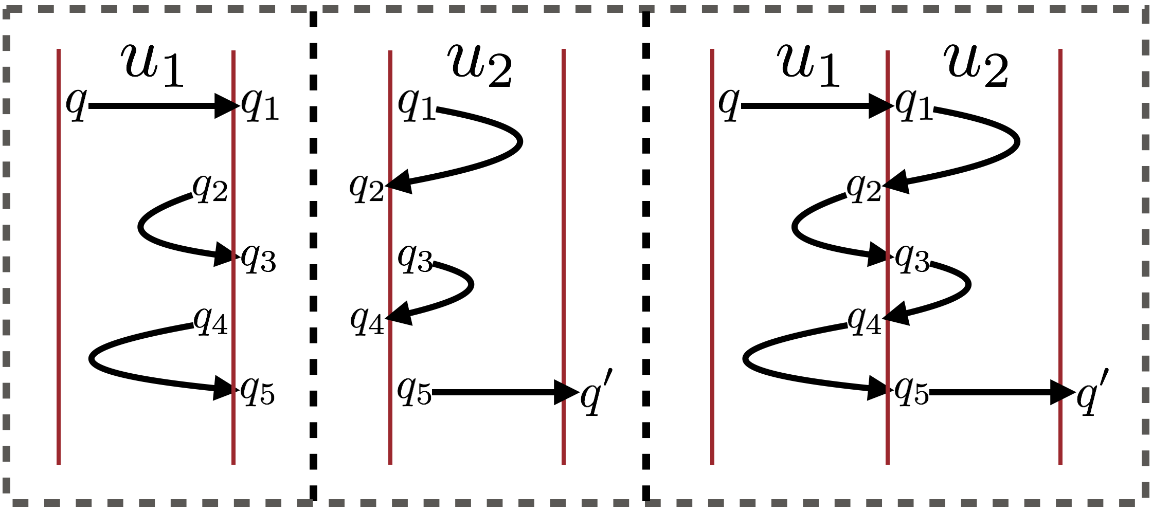
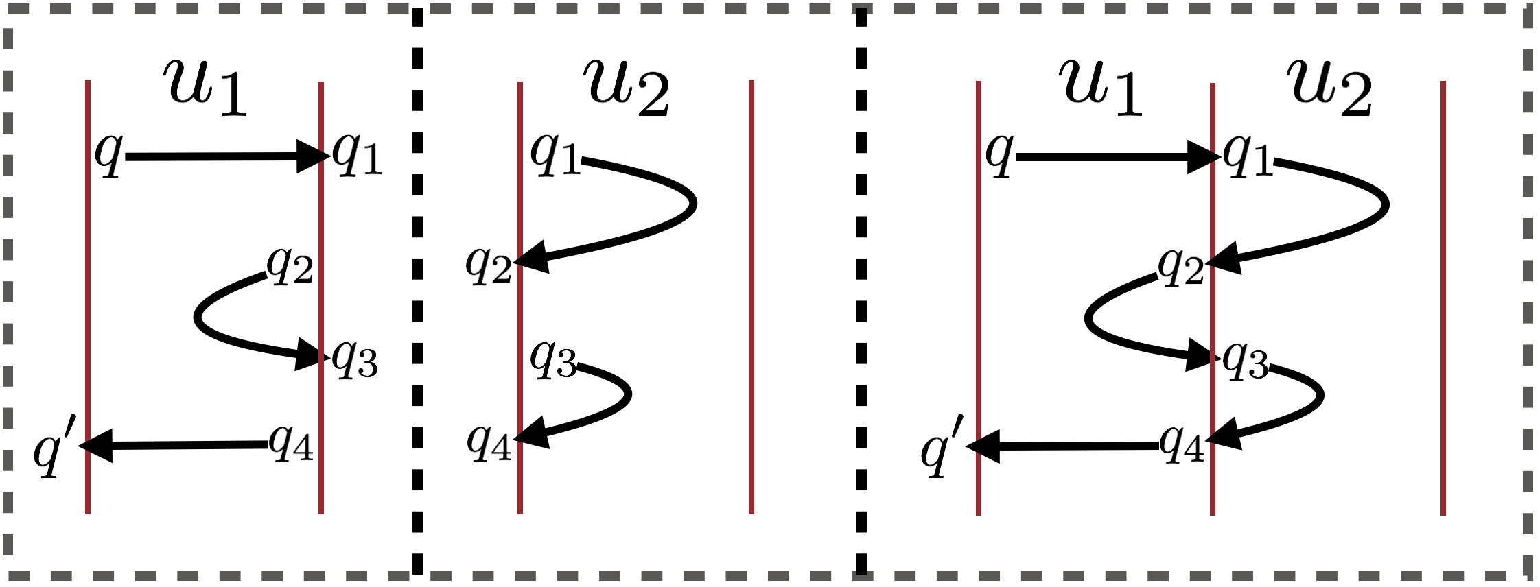
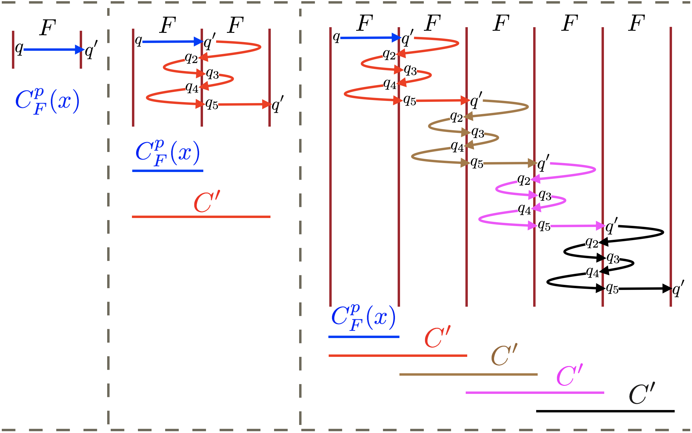
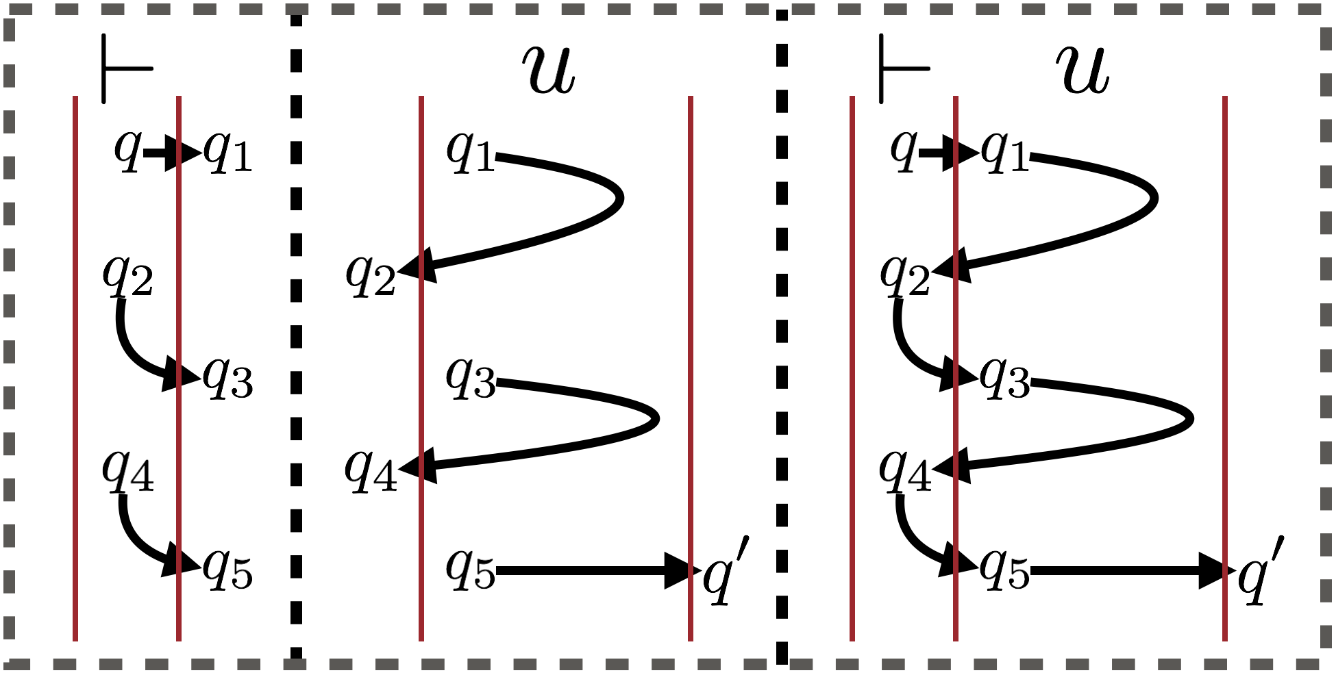
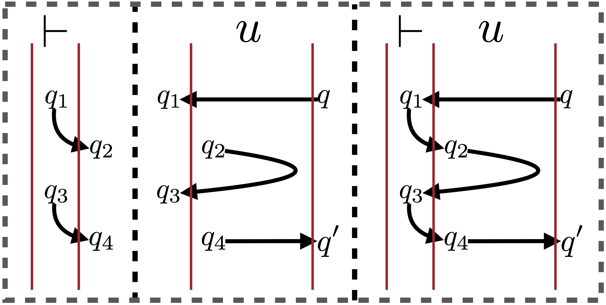
Figure 9:

We now define RTEs corresponding to the left part of the computation of the $\omega$-2DMT_la $\mathcal{A}$, i.e., on some input ${\vdash}u$ consisting of the left end-marker and some finite word $u\in\Sigma^{+}$. As before, the look-ahead is determined by the state of the $\mathsf{BDBA}$ ${\mathcal{B}}$.

Lemma 3.17.

Let $F$ be an $\varepsilon$-free $\mathsf{Tr}$-good rational expression. For each state $p\in P$ and $q\in Q$, there is a unique state $q^{\prime}\in Q$ and an RTE $C_{{\vdash}F}^{p}(q,\rightarrow,q^{\prime})$ (resp. $C_{{\vdash}F}^{p}(q,\mathrel{\leavevmode\resizebox{1.5pt}{0.8pt}{\rotatebox[origin={c}]{90.0}{$\curvearrowleft$}}},q^{\prime})$) such that the following invariants hold:

1. $\mathcal{L}(F)=\mathsf{dom}(C_{{\vdash}F}^{p}(q,\rightarrow,q^{\prime}))$ (resp. $\mathcal{L}(F)=\mathsf{dom}(C_{{\vdash}F}^{p}(q,\mathrel{\leavevmode\resizebox{1.5pt}{0.8pt}{\rotatebox[origin={c}]{90.0}{$\curvearrowleft$}}},q^{\prime}))$),

2. for each $u\in\mathcal{L}(F)$, $[\![C_{{\vdash}F}^{p}(q,\rightarrow,q^{\prime})]\!](u)$ (resp. $[\![C_{{\vdash}F}^{p}(q,\mathrel{\leavevmode\resizebox{1.5pt}{0.8pt}{\rotatebox[origin={c}]{90.0}{$\curvearrowleft$}}},q^{\prime})]\!](u)$) is the output produced by $\widetilde{\mathcal{A}}$ on $\widetilde{{\vdash}u}^{p}$ when starting on the left (resp. right) in state $q$ until it exists on the right in state $q^{\prime}$.

Proof 3.18.

Let $\sigma=(r^{p},b^{p},s^{p})_{p\in P}=\mathsf{Tr}(F)$. We fix some state $p\in P$. For all words $u\in\mathcal{L}(F)$, we have $\widetilde{{\vdash}u}^{p}=({\vdash},r^{p})\widetilde{u}^{p}$. Let $s_{\vdash}^{p}$ be the set of steps $(q,\rightarrow,q^{\prime}),(q,\mathrel{\leavevmode\resizebox{1.5pt}{0.8pt}{\rotatebox[origin={c}]{90.0}{$\curvearrowleft$}}},q^{\prime})$ such that $\widetilde{\delta}(q,({\vdash},r^{p}))=(q^{\prime},\gamma_{q}^{p},+1)$ in $\widetilde{\mathcal{A}}$.

For each $q\in Q$, there is a unique sequence of steps $x_{1}=(q,\rightarrow,q_{1})$, $x_{2}=(q_{1},\mathrel{\leavevmode\resizebox{1.5pt}{0.8pt}{\rotatebox[origin={c}]{-90.0}{$\curvearrowright$}}},X_{2},q_{2})$, $x_{3}=(q_{2},\mathrel{\leavevmode\resizebox{1.5pt}{0.8pt}{\rotatebox[origin={c}]{90.0}{$\curvearrowleft$}}},q_{3})$, $x_{4}=(q_{3},\mathrel{\leavevmode\resizebox{1.5pt}{0.8pt}{\rotatebox[origin={c}]{-90.0}{$\curvearrowright$}}},X_{4},q_{4})$, …, $x_{i}=(q_{i-1},\mathrel{\leavevmode\resizebox{1.5pt}{0.8pt}{\rotatebox[origin={c}]{90.0}{$\curvearrowleft$}}},q_{i})$, $x_{i+1}=(q_{i},\rightarrow,X_{i+1},q^{\prime})$ with $i\geq 1$, $x_{1},x_{3},\ldots,x_{i}\in s_{\vdash}^{p}$ and $x_{2},x_{4},\ldots,x_{i+1}\in s^{p}$ (see Figure 9 bottom left). We define

$$C_{{\vdash}F}^{p}(q,\rightarrow,q^{\prime})=\gamma_{q}^{p}\odot C_{F}^{p}(x_{2})\odot\gamma_{q_{2}}^{p}\odot C_{F}^{p}(x_{4})\odot\cdots\odot\gamma_{q_{i-1}}^{p}\odot C_{F}^{p}(x_{i+1})\,.$$

Using Lemma 3.15, we can show that $\mathcal{L}(F)=\mathsf{dom}(C_{{\vdash}F}^{p}(q,\rightarrow,q^{\prime}))$ and also that for each $u\in\mathcal{L}(F)$, $[\![C_{{\vdash}F}^{p}(q,\rightarrow,q^{\prime})]\!](u)$ is the output produced by $\widetilde{\mathcal{A}}$ on $\widetilde{{\vdash}u}^{p}$ when starting on the left in state $q$ until it exists on the right in state $q^{\prime}$.

For each $q\in Q$, there is a unique sequence of steps $x_{1}=(q,\leftarrow,X_{1},q_{1})$, $x_{2}=(q_{1},\mathrel{\leavevmode\resizebox{1.5pt}{0.8pt}{\rotatebox[origin={c}]{90.0}{$\curvearrowleft$}}},q_{2})$, $x_{3}=(q_{2},\mathrel{\leavevmode\resizebox{1.5pt}{0.8pt}{\rotatebox[origin={c}]{-90.0}{$\curvearrowright$}}},X_{3},q_{3})$, $x_{4}=(q_{3},\mathrel{\leavevmode\resizebox{1.5pt}{0.8pt}{\rotatebox[origin={c}]{90.0}{$\curvearrowleft$}}},q_{4})$, …, $x_{i}=(q_{i-1},\mathrel{\leavevmode\resizebox{1.5pt}{0.8pt}{\rotatebox[origin={c}]{90.0}{$\curvearrowleft$}}},q_{i})$, $x_{i+1}=(q_{i},\rightarrow,X_{i+1},q^{\prime})$ with $i\geq 2$, $x_{2},x_{4},\ldots,x_{i}\in s_{\vdash}^{p}$ and $x_{1},x_{3},\ldots,x_{i+1}\in s^{p}$ (see Figure 9 bottom right). We define

$$C_{{\vdash}F}^{p}(q,\mathrel{\leavevmode\resizebox{1.5pt}{0.8pt}{\rotatebox[origin={c}]{90.0}{$\curvearrowleft$}}},q^{\prime})=C_{F}^{p}(x_{1})\odot\gamma_{q_{1}}^{p}\odot C_{F}^{p}(x_{3})\odot\gamma_{q_{3}}^{p}\odot\cdots\odot\gamma_{q_{i-1}}^{p}\odot C_{F}^{p}(x_{i+1})\,.$$

Using Lemma 3.15, we can show that $\mathcal{L}(F)=\mathsf{dom}(C_{{\vdash}F}^{p}(q,\mathrel{\leavevmode\resizebox{1.5pt}{0.8pt}{\rotatebox[origin={c}]{90.0}{$\curvearrowleft$}}},q^{\prime}))$ and also that for each $u\in\mathcal{L}(F)$, $[\![C_{{\vdash}F}^{p}(q,\mathrel{\leavevmode\resizebox{1.5pt}{0.8pt}{\rotatebox[origin={c}]{90.0}{$\curvearrowleft$}}},q^{\prime})]\!](u)$ is the output produced by $\widetilde{\mathcal{A}}$ on $\widetilde{{\vdash}u}^{p}$ when starting on the right in state $q$ until it exists on the right in state $q^{\prime}$.

Lemma 3.19.

Let $F\cdot G^{\omega}$ be an unambiguous rational expression such that $F$ and $G$ are $\varepsilon$-free $\mathsf{Tr}$-good rational expresions and $\mathsf{Tr}(G)=\sigma=(r^{p},b^{p},s^{p})_{p\in P}$ is an idempotent in the transition monoid $\mathsf{TrM}$ of $(\mathcal{A},{\mathcal{B}})$. We can construct an $\omega$-RTE $C_{FG^{\omega}}$ such that $\mathsf{dom}(C_{FG^{\omega}})=\mathcal{L}(FG^{\omega})\cap\mathsf{dom}(\mathcal{A})$ and for each $w\in\mathsf{dom}(C_{FG^{\omega}})$, $[\![C_{FG^{\omega}}]\!](w)=[\![\mathcal{A}]\!](w)$.

Proof 3.20.

We first show that there exists one and only one state $p\in P$ such that $r^{p}=p$ and $b^{p}=1$. For the existence, consider a word $w=u_{1}u_{2}u_{3}\cdots\in\mathcal{L}(FG^{\omega})$ with $u_{1}\in\mathcal{L}(F)$ and $u_{n}\in\mathcal{L}(G)$ for all $n\geq 2$. By definition of $\mathsf{BDBA}$ there is a unique final run of ${\mathcal{B}}$ over $w$: $p_{0},u_{1},p_{1},u_{2},p_{2},\ldots$. Let us show first that $p_{n}=p_{1}$ for all $n\geq 1$. Since $\sigma$ is idempotent, we have $\mathsf{Tr}(u_{2}\cdots u_{n+1})=\mathsf{Tr}(u_{n+1})$. Since $p_{1}\xleftarrow{u_{2}\cdots u_{n+1}}p_{n+1}$ and $p_{n}\xleftarrow{u_{n+1}}p_{n+1}$, we deduce that $p_{1}=r^{p_{n+1}}=p_{n}$. This implies $p_{1}=r^{p_{2}}=r^{p_{1}}$. Let $p=p_{1}$ so that $p=r^{p}$ and the final run of ${\mathcal{B}}$ on $w$ is $p_{0},u_{1},p,u_{2},p,\ldots$. Now, for all $n\geq 2$ we have $\mathsf{Tr}(u_{n})=\sigma$ and we deduce that $p\xleftarrow{u_{n}}p$ visits a final state from $\mathsf{Fin}$ iff $b^{p}=1$. Since the run is accepting, we deduce that indeed $b^{p}=1$. To prove the unicity, let $p\in P$ with $p=r^{p}$ and $b^{p}=1$. Let $v\in\mathcal{L}(G)$. We have $p\xleftarrow{v}p$ and this subrun visits a final state from $\mathsf{Fin}$. Therefore, $p,v,p,v,p,v,p,\ldots$ is a final run of ${\mathcal{B}}$ on $v^{\omega}$. Since ${\mathcal{B}}$ is $\mathsf{BDBA}$, there is a unique final run of ${\mathcal{B}}$ on $v^{\omega}$, which proves the unicity of $p$.

We apply Lemma 3.17. We denote by $s^{\prime}_{{\vdash}F}$ the set of triples $(q,d,q^{\prime})\in Q\times\{\rightarrow,\mathrel{\leavevmode\resizebox{1.5pt}{0.8pt}{\rotatebox[origin={c}]{90.0}{$\curvearrowleft$}}}\}\times Q$ such that the RTE $C_{{\vdash}F}^{p}(q,d,q^{\prime})$ is defined.

Starting from the initial state $q_{0}$ of $\mathcal{A}$, there exists a unique sequence of steps $x^{\prime}_{1}=(q_{0},\rightarrow,q^{\prime}_{1})$, $x^{\prime}_{2}=(q^{\prime}_{1},\mathrel{\leavevmode\resizebox{1.5pt}{0.8pt}{\rotatebox[origin={c}]{-90.0}{$\curvearrowright$}}},X^{\prime}_{2},q^{\prime}_{2})$, $x^{\prime}_{3}=(q^{\prime}_{2},\mathrel{\leavevmode\resizebox{1.5pt}{0.8pt}{\rotatebox[origin={c}]{90.0}{$\curvearrowleft$}}},q^{\prime}_{3})$, $x^{\prime}_{4}=(q^{\prime}_{3},\mathrel{\leavevmode\resizebox{1.5pt}{0.8pt}{\rotatebox[origin={c}]{-90.0}{$\curvearrowright$}}},X^{\prime}_{4},q^{\prime}_{4})$, …, $x^{\prime}_{i}=(q^{\prime}_{i-1},\mathrel{\leavevmode\resizebox{1.5pt}{0.8pt}{\rotatebox[origin={c}]{90.0}{$\curvearrowleft$}}},q^{\prime}_{i})$, $x^{\prime}_{i+1}=(q^{\prime}_{i},\rightarrow,X^{\prime}_{i+1},q)$ with $i\geq 1$, $x^{\prime}_{1},x^{\prime}_{3},\ldots,x^{\prime}_{i}\in s^{\prime}_{{\vdash}F}$ and $x^{\prime}_{2},x^{\prime}_{4},\ldots,x^{\prime}_{i+1}\in s^{p}$. We define

$$C_{1} =\big{(}C_{{\vdash}F}^{p}(x^{\prime}_{1})\mathbin{{\boxdot}}C_{G}^{p}(x^{\prime}_{2})\big{)}\odot\big{(}C_{{\vdash}F}^{p}(x^{\prime}_{3})\mathbin{{\boxdot}}C_{G}^{p}(x^{\prime}_{4})\big{)}\odot\cdots\odot\big{(}C_{{\vdash}F}^{p}(x^{\prime}_{i})\mathbin{{\boxdot}}C_{G}^{p}(x^{\prime}_{i+1})\big{)}$$

$$C_{2} =C_{1}\mathbin{{\boxdot}}({G^{\omega}}\,?\,{\varepsilon}:{\bot})\,.$$

We have $\mathsf{dom}(C_{1})=FG$ and $\widetilde{{\vdash}u_{1}u_{2}}^{p}=\widetilde{{\vdash}u_{1}}^{p}\widetilde{u_{2}}^{p}$ for all $u_{1}\in F$ and $u_{2}\in G$. Moreover, $[\![C_{1}]\!](u_{1}u_{2})$ is the output produced by $\widetilde{\mathcal{A}}$ on $\widetilde{{\vdash}u_{1}u_{2}}^{p}$ when starting on the left in the initial state $q_{0}$ until it exists on the right in state $q$. Now, $C_{2}$ is an $\omega$-RTE with $\mathsf{dom}(C_{2})=FG^{\omega}$ and for all $w=u_{1}u_{2}u_{3}\ldots\in FG^{\omega}$ with $u_{1}\in F$ and $u_{n}\in G$ for all $n>1$, we have $[\![C_{2}]\!](w)=[\![C_{1}]\!](u_{1}u_{2})\in\Gamma^{*}$.

Now, we distinguish two cases. First, assume that there is a step $x=(q,\rightarrow,X,q^{\prime})\in s^{p}$. Since $\sigma$ is idempotent, so is $s^{p}$, and since $x^{\prime}_{i+1}=(q^{\prime}_{i},\rightarrow,X^{\prime}_{i+1},q)\in s^{p}$ we deduce that $q^{\prime}=q$. Therefore, the unique run of $\widetilde{\mathcal{A}}$ on $\widetilde{{\vdash}w}=\widetilde{{\vdash}u_{1}}^{p}\widetilde{u_{2}}^{p}\widetilde{u_{3}}^{p}\cdots$ follows the steps $x^{\prime}_{1}x^{\prime}_{2}\cdots x^{\prime}_{i}x^{\prime}_{i+1}xxx\cdots$. Hence, the set of states visited infinitely often along this run is $X$ and the run is accepting iff $X\in\mathcal{F}$ is a Muller set. Therefore, if $X\notin\mathcal{F}$ we have $FG^{\omega}\cap\mathsf{dom}(\mathcal{A})=\emptyset$ and we set $C_{FG^{\omega}}=\bot$. Now, if $X\in\mathcal{F}$ we have $FG^{\omega}\subseteq\mathsf{dom}(\mathcal{A})$ and we set

$$C_{FG^{\omega}}=C_{2}\odot\big{(}({FG}\,?\,{\varepsilon}:{\bot})\mathbin{{\boxdot}}C_{G}^{p}(x)^{\omega}\big{)}\,.$$

We have $\mathsf{dom}(C_{FG^{\omega}})=FG^{\omega}$ and for all $w=u_{1}u_{2}u_{3}\ldots\in FG^{\omega}$ with $u_{1}\in F$ and $u_{n}\in G$ for all $n>1$, we have

$$[\![C_{FG^{\omega}}]\!](w)=[\![C_{1}]\!](u_{1}u_{2})[\![C_{G}^{p}(x)]\!](u_{3})[\![C_{G}^{p}(x)]\!](u_{4})\cdots\,.$$

By ($\mathsf{J}_{2}$), we know that for all $n\geq 3$, $[\![C_{G}^{p}(x)]\!](u_{n})$ is the output produced by $\widetilde{\mathcal{A}}$ when running step $x=(q,\rightarrow,X,q)$ on $\widetilde{u_{n}}^{p}$. We deduce that $[\![C_{FG^{\omega}}]\!](w)=[\![\widetilde{\mathcal{A}}]\!](\widetilde{{\vdash}w})=[\![\mathcal{A}]\!](w)$ as desired.

The second case is when the unique step $x_{1}=(q,\mathrel{\leavevmode\resizebox{1.5pt}{0.8pt}{\rotatebox[origin={c}]{-90.0}{$\curvearrowright$}}},X_{1},q_{1})$ in $s^{p}$ which starts from the left in state $q$ exits on the left. Since $s^{p}$ is idempotent and $x^{\prime}_{i+1}=(q^{\prime}_{i},\rightarrow,X^{\prime}_{i+1},q)\in s^{p}$, by definition of the product $s^{p}\cdot s^{p}$, there is a unique sequence of steps $x_{2}=(q_{1},\mathrel{\leavevmode\resizebox{1.5pt}{0.8pt}{\rotatebox[origin={c}]{90.0}{$\curvearrowleft$}}},X_{2},q_{2})$, $x_{3}=(q_{2},\mathrel{\leavevmode\resizebox{1.5pt}{0.8pt}{\rotatebox[origin={c}]{-90.0}{$\curvearrowright$}}},X_{3},q_{3})$, …, $x_{j}=(q_{j-1},\mathrel{\leavevmode\resizebox{1.5pt}{0.8pt}{\rotatebox[origin={c}]{90.0}{$\curvearrowleft$}}},X_{j},q_{j})$, $x_{j+1}=(q_{j},\rightarrow,X_{j+1},q)$ in $s^{p}$ with $j\geq 2$. Therefore, for all $w=u_{1}u_{2}u_{3}\ldots\in FG^{\omega}$ with $u_{1}\in F$ and $u_{n}\in G$ for all $n>1$, the unique run of $\widetilde{\mathcal{A}}$ on $\widetilde{{\vdash}w}=\widetilde{{\vdash}u_{1}}^{p}\widetilde{u_{2}}^{p}\widetilde{u_{3}}^{p}\cdots$ follows the steps $x^{\prime}_{1}x^{\prime}_{2}\cdots x^{\prime}_{i}x^{\prime}_{i+1}(x_{1}x_{2}x_{3}\cdots x_{j}x_{j+1})^{\omega}$. Hence, the set of states visited infinitely often along this run is $X=X_{1}\cup X_{2}\cup\cdots\cup X_{j+1}$. We deduce that the run is accepting iff $X\in\mathcal{F}$ is a Muller set. Therefore, if $X\notin\mathcal{F}$ we have $FG^{\omega}\cap\mathsf{dom}(\mathcal{A})=\emptyset$ and we set $C_{FG^{\omega}}=\bot$. Now, if $X\in\mathcal{F}$ we have $FG^{\omega}\subseteq\mathsf{dom}(\mathcal{A})$ and we set

$$C_{3} =\big{(}({G}\,?\,{\varepsilon}:{\bot})\mathbin{{\boxdot}}C_{G}^{p}(x_{1})\big{)}\odot\big{(}C_{G}^{p}(x_{2})\mathbin{{\boxdot}}C_{G}^{p}(x_{3})\big{)}\odot\cdots\odot\big{(}C_{G}^{p}(x_{j})\mathbin{{\boxdot}}C_{G}^{p}(x_{j+1})\big{)}$$

$$C_{FG^{\omega}} =C_{2}\odot\big{(}({F}\,?\,{\varepsilon}:{\bot})\mathbin{{\boxdot}}[G,C_{3}]^{2\omega}\big{)}\,.$$

We have $\mathsf{dom}(C_{FG^{\omega}})=FG^{\omega}$ and for all $w=u_{1}u_{2}u_{3}\ldots\in FG^{\omega}$ with $u_{1}\in F$ and $u_{n}\in G$ for all $n>1$, we have

$$[\![C_{FG^{\omega}}]\!](w)=[\![C_{1}]\!](u_{1}u_{2})[\![C_{3}]\!](u_{2}u_{3})[\![C_{3}]\!](u_{3}u_{4})\cdots\,.$$

Using ($\mathsf{J}_{2}$), we can check that this is the output produced by $\widetilde{\mathcal{A}}$ when running on $\widetilde{{\vdash}w}$. We deduce that $[\![C_{FG^{\omega}}]\!](w)=[\![\widetilde{\mathcal{A}}]\!](\widetilde{{\vdash}w})=[\![\mathcal{A}]\!](w)$ as desired.

We are now ready to prove that $\omega$-2DMT_la are no more expressive than $\omega$-RTEs.

Proof 3.21 (Proof of Theorem 3.6 (2)).

We use the notations of the previous sections, in particular for the $\omega$-2DMT_la $\mathcal{A}$, the $\mathsf{BDBA}$ ${\mathcal{B}}$. We apply Theorem 3.14 to the canonical morphism $\mathsf{Tr}$ from $\Sigma^{*}$ to the transition monoid $\mathsf{TrM}$ of $(\mathcal{A},{\mathcal{B}})$. We obtain an unambiguous rational expression $G=\bigcup_{k=1}^{m}F_{k}\cdot G_{k}^{\omega}$ over $\Sigma$ such that $\mathcal{L}(G)=\Sigma^{\omega}$ and for all $1\leq k\leq m$ the expressions $F_{k}$ and $G_{k}$ are $\varepsilon$-free $\mathsf{Tr}$-good rational expressions and $\sigma_{G_{k}}$ is an idempotent, where $\mathsf{Tr}(G_{k})=\{\sigma_{G_{k}}\}$. For each $1\leq k\leq m$, let $C_{k}=C_{F_{k}G_{k}^{\omega}}$ be the $\omega$-RTE given by Lemma 3.19. We define the final $\omega$-RTE as

$$C={F_{1}G_{1}^{\omega}}\,?\,{C_{1}}:{({F_{2}G_{2}^{\omega}}\,?\,{C_{2}}:{\cdots({F_{m-1}G_{m-1}^{\omega}}\,?\,{C_{{m-1}}}:{C_{m}})})}\,.$$

From Lemma 3.19, we can easily check that $\mathsf{dom}(C)=\mathsf{dom}(\mathcal{A})$ and $[\![C]\!](w)=[\![\mathcal{A}]\!](w)$ for all $w\in\mathsf{dom}(C)$.

4 Conclusion

The main contribution of the paper is to give a characterisation of regular string transductions using some combinators, giving rise to regular transducer expressions (RTE). Our proof uniformly works well for finite and infinite string transformations. RTE are a succint specification mechanism for regular transformations just like regular expressions are for regular languages. It is worthwhile to consider extensions of our technique to regular tree transformations, or in other settings where more involved primitives such as sorting or counting are needed. The minimality of our combinators in achieving expressive completeness, as well as computing complexity measures for the conversion between RTEs and two-way transducers are open.

Appendix A Examples

A.1 More details on the Example in the Introduction

We continue with the computation of the RTE $C_{E_{3}}(q_{0},\rightarrow,q_{2})$ for $E_{3}=[(ba^{+})^{3}]^{+}b\subseteq\mathsf{dom}({\mathcal{A}})$. This involves the use of the 2-chained Kleene-plus.

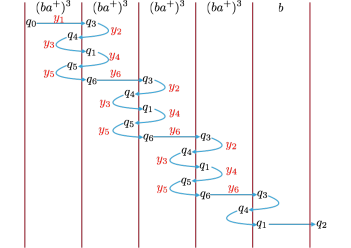
Figure 10: run of a word in $E_{3}=[(ba^{+})^{3}]^{+}b$

We want to compute the RTE for the step $(q_{0},\rightarrow,q_{2})$ on a word $u\in E_{3}$. It can be decomposed as shown in Figure 10. Unlike the case of $E_{2}$, we have to use the 2-chained Kleene plus. Let $F=(ba^{+})^{3}$ so that $E_{3}=F^{+}b$. We have (see Figure 10),

$$C_{E_{3}}(q_{0},\rightarrow,q_{2})=(C_{F^{+}}(q_{0},\rightarrow,q_{3})\mathbin{{\boxdot}}C_{b}(q_{3},\mathrel{\leavevmode\resizebox{1.5pt}{0.8pt}{\rotatebox[origin={c}]{-90.0}{$\curvearrowright$}}},q_{4}))\odot(C_{F^{+}}(q_{4},\mathrel{\leavevmode\resizebox{1.5pt}{0.8pt}{\rotatebox[origin={c}]{90.0}{$\curvearrowleft$}}},q_{1})\mathbin{{\boxdot}}C_{b}(q_{1},\rightarrow,q_{2}))\,.$$

We know that $C_{b}(q_{3},\mathrel{\leavevmode\resizebox{1.5pt}{0.8pt}{\rotatebox[origin={c}]{-90.0}{$\curvearrowright$}}},q_{4})=(b/\varepsilon)=C_{b}(q_{1},\rightarrow,q_{2})$ hence it remains to compute $C_{F^{+}}(q_{0},\rightarrow,q_{3})$ and $C_{F^{+}}(q_{4},\mathrel{\leavevmode\resizebox{1.5pt}{0.8pt}{\rotatebox[origin={c}]{90.0}{$\curvearrowleft$}}},q_{1})$. First we define RTEs associated with atomic expressions and steps which are going to be used in constructing $C_{E_{3}}(q_{0},\rightarrow,q_{2})$. They are $C_{b}(q_{3},\mathrel{\leavevmode\resizebox{1.5pt}{0.8pt}{\rotatebox[origin={c}]{-90.0}{$\curvearrowright$}}},q_{4})=C_{b}(q_{6},\rightarrow,q_{1})=C_{b}(q_{1},\rightarrow,q_{2})=C_{b}(q_{5},\rightarrow,q_{6})=(b/\varepsilon)$ and $C_{a^{+}}(q_{2},\rightarrow,q_{3})=C_{a^{+}}(q_{1},\rightarrow,q_{1})={(a/\varepsilon)}^{\scriptstyle{\boxplus}}$, $C_{a^{+}}(q_{4},\leftarrow,q_{4})={(a/a)}^{\scriptstyle{\overleftarrow{\rule{0.0pt}{3.91806pt}\boxplus}}}$, $C_{a^{+}}(q_{5},\leftarrow,q_{5})={(a/b)}^{\scriptstyle{\overleftarrow{\rule{0.0pt}{3.91806pt}\boxplus}}}$. We compute RTE $C_{F}(x)$ for the relevant steps $x$ in the monoid element $X=\mathsf{Tr}(F)$. $F$ is an unambiguous catenation of $E_{2}=ba^{+}ba^{+}b$ with $a^{+}$ and from Figure 2, it can be seen that:

1. For $y_{1}=(q_{0},\rightarrow,q_{3})$

   $$C_{F}(y_{1}) =C_{E_{2}}(q_{0},\rightarrow,q_{2})\mathbin{{\boxdot}}C_{a^{+}}(q_{2},\rightarrow,q_{3})$$

   $$=\big{(}(b/\varepsilon)\mathbin{{\overleftarrow{\rule{0.0pt}{5.59721pt}\boxdot}}}{(a/b)}^{\scriptstyle{\overleftarrow{\rule{0.0pt}{3.91806pt}\boxplus}}}\mathbin{{\overleftarrow{\rule{0.0pt}{5.59721pt}\boxdot}}}(b/\varepsilon)\mathbin{{\overleftarrow{\rule{0.0pt}{5.59721pt}\boxdot}}}{(a/a)}^{\scriptstyle{\overleftarrow{\rule{0.0pt}{3.91806pt}\boxplus}}}\big{)}\mathbin{{\boxdot}}(b/\varepsilon)\mathbin{{\boxdot}}{(a/\varepsilon)}^{\scriptstyle{\boxplus}}$$

   where $C_{E_{2}}(q_{0},\rightarrow,q_{2})$ has been computed in Section 1.
   For example, $[\![C_{F}(y_{1})]\!](ba^{m_{1}}ba^{m_{2}}ba^{m_{3}})=a^{m_{2}}b^{m_{1}}$.

2. Continuing with the computation for $(ba^{+})^{3}$ as in Figure 10, for $y_{2}=(q_{3},\mathrel{\leavevmode\resizebox{1.5pt}{0.8pt}{\rotatebox[origin={c}]{-90.0}{$\curvearrowright$}}},q_{4})$, we take the Cauchy product of $C_{b}(q_{3},\mathrel{\leavevmode\resizebox{1.5pt}{0.8pt}{\rotatebox[origin={c}]{-90.0}{$\curvearrowright$}}},q_{4})$ with $({a^{+}ba^{+}ba^{+}}\,?\,{\varepsilon}:{\bot})$.

   $$C_{F}(y_{2}) =C_{b}(q_{3},\mathrel{\leavevmode\resizebox{1.5pt}{0.8pt}{\rotatebox[origin={c}]{-90.0}{$\curvearrowright$}}},q_{4})\mathbin{{\boxdot}}({a^{+}ba^{+}ba^{+}}\,?\,{\varepsilon}:{\bot})\approx({(ba^{+})^{3}}\,?\,{\varepsilon}:{\bot})$$

   $[\![C_{F}(y_{2})]\!](ba^{m_{1}}ba^{m_{2}}ba^{m_{3}})=\varepsilon$.

3. For $y_{3}=(q_{4},\mathrel{\leavevmode\resizebox{1.5pt}{0.8pt}{\rotatebox[origin={c}]{90.0}{$\curvearrowleft$}}},q_{1})$, we have

   $$C_{F}(y_{3}) =({ba^{+}}\,?\,{\varepsilon}:{\bot})\mathbin{{\overleftarrow{\rule{0.0pt}{5.59721pt}\boxdot}}}C_{ba^{+}ba^{+}}(y_{3})$$

   $$=({ba^{+}}\,?\,{\varepsilon}:{\bot})\mathbin{{\overleftarrow{\rule{0.0pt}{5.59721pt}\boxdot}}}\big{(}(b/\varepsilon)\mathbin{{\overleftarrow{\rule{0.0pt}{5.59721pt}\boxdot}}}{(a/b)}^{\scriptstyle{\overleftarrow{\rule{0.0pt}{3.91806pt}\boxplus}}}\mathbin{{\overleftarrow{\rule{0.0pt}{5.59721pt}\boxdot}}}(b/\varepsilon)\mathbin{{\overleftarrow{\rule{0.0pt}{5.59721pt}\boxdot}}}{(a/a)}^{\scriptstyle{\overleftarrow{\rule{0.0pt}{3.91806pt}\boxplus}}}\big{)}$$

   $$\approx({ba^{+}b}\,?\,{\varepsilon}:{\bot})\mathbin{{\boxdot}}\big{(}{(a/b)}^{\scriptstyle{\overleftarrow{\rule{0.0pt}{3.91806pt}\boxplus}}}\mathbin{{\overleftarrow{\rule{0.0pt}{5.59721pt}\boxdot}}}(b/\varepsilon)\mathbin{{\overleftarrow{\rule{0.0pt}{5.59721pt}\boxdot}}}{(a/a)}^{\scriptstyle{\overleftarrow{\rule{0.0pt}{3.91806pt}\boxplus}}}\big{)}$$

   where $C_{ba^{+}ba^{+}}(y_{3})$ is already computed in Section 1.
   As an example, $[\![C_{F}(y_{3})]\!](ba^{m_{1}}ba^{m_{2}}ba^{m_{3}})=a^{m_{3}}b^{m_{2}}$.

4. For $y_{4}=(q_{1},\mathrel{\leavevmode\resizebox{1.5pt}{0.8pt}{\rotatebox[origin={c}]{-90.0}{$\curvearrowright$}}},q_{5})$, it is similar to the $C_{E}(y)$ computed for $C_{E_{2}}$ in Section 1. Here we have

   $$C_{F}(y_{4}) =C_{ba^{+}b}(y_{4})\mathbin{{\boxdot}}({a^{+}ba^{+}}\,?\,{\varepsilon}:{\bot})$$

   $$=\big{(}(C_{b}(q_{1},\rightarrow,q_{2})\mathbin{{\boxdot}}C_{a^{+}}(q_{2},\rightarrow,q_{3})\mathbin{{\boxdot}}(b/\varepsilon))\odot{}$$

   $$\leavevmode\nobreak\ \leavevmode\nobreak\ \leavevmode\nobreak\ \leavevmode\nobreak\ \leavevmode\nobreak\ \leavevmode\nobreak\ (C_{b}(q_{4},\leftarrow,q_{5})\mathbin{{\overleftarrow{\rule{0.0pt}{5.59721pt}\boxdot}}}C_{a^{+}}(q_{4},\leftarrow,q_{4})\mathbin{{\overleftarrow{\rule{0.0pt}{5.59721pt}\boxdot}}}C_{b}(q_{3},\mathrel{\leavevmode\resizebox{1.5pt}{0.8pt}{\rotatebox[origin={c}]{-90.0}{$\curvearrowright$}}},q_{4}))\big{)}\mathbin{{\boxdot}}({a^{+}ba^{+}}\,?\,{\varepsilon}:{\bot})$$

   $$=(((b/\varepsilon)\mathbin{{\boxdot}}{(a/\varepsilon)}^{\scriptstyle{\boxplus}}\mathbin{{\boxdot}}(b/\varepsilon))\odot((b/\varepsilon)\mathbin{{\overleftarrow{\rule{0.0pt}{5.59721pt}\boxdot}}}{(a/a)}^{\scriptstyle{\overleftarrow{\rule{0.0pt}{3.91806pt}\boxplus}}}\mathbin{{\overleftarrow{\rule{0.0pt}{5.59721pt}\boxdot}}}(b/\varepsilon)))\mathbin{{\boxdot}}({a^{+}ba^{+}}\,?\,{\varepsilon}:{\bot})$$

   $$\approx\big{(}(b/\varepsilon)\mathbin{{\overleftarrow{\rule{0.0pt}{5.59721pt}\boxdot}}}{(a/a)}^{\scriptstyle{\overleftarrow{\rule{0.0pt}{3.91806pt}\boxplus}}}\mathbin{{\overleftarrow{\rule{0.0pt}{5.59721pt}\boxdot}}}(b/\varepsilon)\big{)}\mathbin{{\boxdot}}({a^{+}ba^{+}}\,?\,{\varepsilon}:{\bot})$$

   As an example, $[\![C_{F}(y_{4})]\!](ba^{m_{1}}ba^{m_{2}}ba^{m_{3}})=a^{m_{1}}$.

5. For $y_{5}=(q_{5},\mathrel{\leavevmode\resizebox{1.5pt}{0.8pt}{\rotatebox[origin={c}]{90.0}{$\curvearrowleft$}}},q_{6})$, in the computation of $C_{F}(y_{5})$ we need $C_{ba^{+}}(y_{5})$. Thus, we compute $C_{ba^{+}}(y_{5})$ below whose computation is similar to $C_{E}(y)$ computed in Section 1.

   $$C_{ba^{+}}(y_{5}) =((b/\varepsilon)\mathbin{{\overleftarrow{\rule{0.0pt}{5.59721pt}\boxdot}}}C_{a^{+}}(q_{5},\leftarrow,q_{5}))\odot(C_{b}(q_{5},\rightarrow,q_{6})\mathbin{{\boxdot}}C_{a^{+}}(q_{6},\rightarrow,q_{6}))$$

   $$=((b/\varepsilon)\mathbin{{\overleftarrow{\rule{0.0pt}{5.59721pt}\boxdot}}}{(a/b)}^{\scriptstyle{\overleftarrow{\rule{0.0pt}{3.91806pt}\boxplus}}})\odot((b/\varepsilon)\mathbin{{\boxdot}}{(a/\varepsilon)}^{\scriptstyle{\boxplus}})\approx(b/\varepsilon)\mathbin{{\overleftarrow{\rule{0.0pt}{5.59721pt}\boxdot}}}{(a/b)}^{\scriptstyle{\overleftarrow{\rule{0.0pt}{3.91806pt}\boxplus}}}$$

   We can compute $C_{F}(y_{5})$ as

   $$C_{F}(y_{5}) =({ba^{+}ba^{+}}\,?\,{\varepsilon}:{\bot})\mathbin{{\boxdot}}C_{ba^{+}}(y_{5})\approx({ba^{+}ba^{+}b}\,?\,{\varepsilon}:{\bot})\mathbin{{\overleftarrow{\rule{0.0pt}{5.59721pt}\boxdot}}}{(a/b)}^{\scriptstyle{\overleftarrow{\rule{0.0pt}{3.91806pt}\boxplus}}}$$

   As an example, $[\![C_{F}(y_{5})]\!](ba^{m_{1}}ba^{m_{2}}ba^{m_{3}})=b^{m_{3}}$.

6. For $y_{6}=(q_{6},\rightarrow,q_{3})$, the computation of $C_{F}(y_{6})$ is similar to $C_{ba^{+}ba^{+}}(q_{0},\rightarrow,q_{2})$ in Section 1. We need $C_{ba^{+}ba^{+}}(q_{6},\rightarrow,q_{3})$ and $C_{ba^{+}ba^{+}b}(q_{6},\rightarrow,q_{2})$. We see the computation of these below step by step.

   $$C_{ba^{+}ba^{+}}(q_{6},\rightarrow,q_{3}) =C_{b}(q_{6},\rightarrow,q_{1})\mathbin{{\boxdot}}C_{a^{+}}(q_{1},\rightarrow,q_{1})\mathbin{{\boxdot}}C_{b}(q_{1},\rightarrow,q_{2})\mathbin{{\boxdot}}C_{a^{+}}(q_{2},\rightarrow,q_{3})$$

   $$=(b/\varepsilon)\mathbin{{\boxdot}}{(a/\varepsilon)}^{\scriptstyle{\boxplus}}\mathbin{{\boxdot}}(b/\varepsilon)\mathbin{{\boxdot}}{(a/\varepsilon)}^{\scriptstyle{\boxplus}}\approx({ba^{+}ba^{+}}\,?\,{\varepsilon}:{\bot})$$

   $$C_{ba^{+}ba^{+}b}(q_{6},\rightarrow,q_{2}) =(C_{ba^{+}ba^{+}}(q_{6},\rightarrow,q_{3})\mathbin{{\boxdot}}C_{b}(q_{3},\mathrel{\leavevmode\resizebox{1.5pt}{0.8pt}{\rotatebox[origin={c}]{-90.0}{$\curvearrowright$}}},q_{4}))\odot(C_{ba^{+}ba^{+}}(q_{4},\mathrel{\leavevmode\resizebox{1.5pt}{0.8pt}{\rotatebox[origin={c}]{90.0}{$\curvearrowleft$}}},q_{1})\mathbin{{\boxdot}}C_{b}(q_{1},\rightarrow,q_{2}))$$

   $$\approx({ba^{+}ba^{+}b}\,?\,{\varepsilon}:{\bot})\odot(((b/\varepsilon)\mathbin{{\overleftarrow{\rule{0.0pt}{5.59721pt}\boxdot}}}{(a/b)}^{\scriptstyle{\overleftarrow{\rule{0.0pt}{3.91806pt}\boxplus}}}\mathbin{{\overleftarrow{\rule{0.0pt}{5.59721pt}\boxdot}}}(b/\varepsilon)\mathbin{{\overleftarrow{\rule{0.0pt}{5.59721pt}\boxdot}}}{(a/a)}^{\scriptstyle{\overleftarrow{\rule{0.0pt}{3.91806pt}\boxplus}}})\mathbin{{\boxdot}}(b/\varepsilon))$$

   $$\approx\big{(}(b/\varepsilon)\mathbin{{\overleftarrow{\rule{0.0pt}{5.59721pt}\boxdot}}}{(a/b)}^{\scriptstyle{\overleftarrow{\rule{0.0pt}{3.91806pt}\boxplus}}}\mathbin{{\overleftarrow{\rule{0.0pt}{5.59721pt}\boxdot}}}(b/\varepsilon)\mathbin{{\overleftarrow{\rule{0.0pt}{5.59721pt}\boxdot}}}{(a/a)}^{\scriptstyle{\overleftarrow{\rule{0.0pt}{3.91806pt}\boxplus}}}\big{)}\mathbin{{\boxdot}}(b/\varepsilon)$$

   Note that $C_{ba^{+}ba^{+}}(q_{4},\mathrel{\leavevmode\resizebox{1.5pt}{0.8pt}{\rotatebox[origin={c}]{90.0}{$\curvearrowleft$}}},q_{1})$ has been computed in Section 1. Now we concatenate with $C_{a^{+}}(q_{2},\rightarrow,q_{3})$ needed in the computation.

   $$C_{F}(y_{6}) =C_{ba^{+}ba^{+}b}(q_{6},\rightarrow,q_{2})\mathbin{{\boxdot}}C_{a^{+}}(q_{2},\rightarrow,q_{3})$$

   $$=\big{(}(b/\varepsilon)\mathbin{{\overleftarrow{\rule{0.0pt}{5.59721pt}\boxdot}}}{(a/b)}^{\scriptstyle{\overleftarrow{\rule{0.0pt}{3.91806pt}\boxplus}}}\mathbin{{\overleftarrow{\rule{0.0pt}{5.59721pt}\boxdot}}}(b/\varepsilon)\mathbin{{\overleftarrow{\rule{0.0pt}{5.59721pt}\boxdot}}}{(a/a)}^{\scriptstyle{\overleftarrow{\rule{0.0pt}{3.91806pt}\boxplus}}}\big{)}\mathbin{{\boxdot}}(b/\varepsilon)\mathbin{{\boxdot}}({a/\varepsilon}^{\scriptstyle{\boxplus}})$$

   $$\approx\big{(}(b/\varepsilon)\mathbin{{\overleftarrow{\rule{0.0pt}{5.59721pt}\boxdot}}}{(a/b)}^{\scriptstyle{\overleftarrow{\rule{0.0pt}{3.91806pt}\boxplus}}}\mathbin{{\overleftarrow{\rule{0.0pt}{5.59721pt}\boxdot}}}(b/\varepsilon)\mathbin{{\overleftarrow{\rule{0.0pt}{5.59721pt}\boxdot}}}{(a/a)}^{\scriptstyle{\overleftarrow{\rule{0.0pt}{3.91806pt}\boxplus}}}\big{)}\mathbin{{\boxdot}}({ba^{+}}\,?\,{\varepsilon}:{\bot})$$

   As an example, $[\![C_{F}(y_{6})]\!](ba^{m_{1}}ba^{m_{2}}ba^{m_{3}})=a^{m_{2}}b^{m_{1}}$.

Now we are in a position to compute RTE $C_{F^{+}}(q_{0},\rightarrow,q_{3})$. As shown in figure10, it is a concatenation of step $y_{1}$ and then steps $y_{2}$, $y_{3}$, $y_{4}$, $y_{5}$ and $y_{6}$ repetitively. Consecutive pairs of $(ba^{+})^{3}$ are needed to compute the RTE and thanks to the 2-chained Kleene plus, we can define the RTE for the same.

$$C_{F^{+}}(y_{1}) =(C_{F}(y_{1})\mathbin{{\boxdot}}({F^{*}}\,?\,{\varepsilon}:{\bot}))\odot[F,C^{\prime}]^{2\scriptstyle{\boxplus}}$$

$$C^{\prime} =(({F}\,?\,{\varepsilon}:{\bot})\mathbin{{\boxdot}}C_{F}(y_{2}))\odot(C_{F}(y_{3})\mathbin{{\boxdot}}C_{F}(y_{4}))\odot(C_{F}(y_{5})\mathbin{{\boxdot}}C_{F}(y_{6}))$$

As an example, $[\![C_{F^{+}}(y_{1})]\!](ba^{m_{1}}ba^{m_{2}}ba^{m_{3}}ba^{m_{4}}ba^{m_{5}}ba^{m_{6}})=a^{m_{2}}b^{m_{1}}a^{m_{3}}b^{m_{2}}a^{m_{4}}b^{m_{3}}a^{m_{5}}b^{m_{4}}$.

Finally, we compute RTE for $y=(q_{0},\rightarrow,q_{2})$ for the expression $E_{3}=[(ba^{+})^{3}]^{+}b$ by concatenating $b$ with the above RTE.

$$C_{E_{3}}(y) =(C_{F^{+}}(q_{0},\rightarrow,q_{3})\mathbin{{\boxdot}}C_{b}(q_{3},\mathrel{\leavevmode\resizebox{1.5pt}{0.8pt}{\rotatebox[origin={c}]{-90.0}{$\curvearrowright$}}},q_{4}))\odot(C_{F^{+}}(q_{4},\mathrel{\leavevmode\resizebox{1.5pt}{0.8pt}{\rotatebox[origin={c}]{90.0}{$\curvearrowleft$}}},q_{1})\mathbin{{\boxdot}}C_{b}(q_{1},\rightarrow,q_{2}))$$

Notice that $C_{F^{+}}(q_{4},\mathrel{\leavevmode\resizebox{1.5pt}{0.8pt}{\rotatebox[origin={c}]{90.0}{$\curvearrowleft$}}},q_{1})=({F^{*}}\,?\,{\varepsilon}:{\bot})\mathbin{{\boxdot}}C_{F}(y_{3})$.

We have already seen that $C_{E_{3}}(y)$ computes the output produced by a successful run on a word $w\in E_{3}$. Applying the RTE as above, we have, for example,

$$[\![C_{E_{3}}(y)]\!](ba^{m_{1}}ba^{m_{2}}ba^{m_{3}}ba^{m_{4}}ba^{m_{5}}ba^{m_{6}}b)=a^{m_{2}}b^{m_{1}}a^{m_{3}}b^{m_{2}}a^{m_{4}}b^{m_{3}}a^{m_{5}}b^{m_{4}}a^{m_{6}}b^{m_{5}}\,.$$

A.2 A Motivating Example

Apart from theoretical interest, regular expressions have great practical utility, being used in search engines, or in search and replace patterns in text processors, or in lexical analysis in compilers. Many programming languages like Java and Python also support regular expressions using a regexp engine, as part of their standard libraries. We believe that our extension of the beautiful theory of regular expressions to regular transducer expressions over both finite and infinite words has many useful applications.

As a specific example, we consider the $\mathsf{dmesg}$ command (see Figure 11 for a sample output) used to write the kernel messages in Linux and other Unix-like operating systems to standard output (which by default is the display screen). The output is often captured in a permanent system logfile via a logging daemon, such as syslog. The kernel is the first part of the operating system that is loaded into memory when a computer boots up. The numerous messages generated by the kernel that appear on the display screen as a computer boots up show the hardware devices that the kernel detects and indicate whether it is able to configure them. $\mathsf{dmesg}$ obtains its data by reading the kernel ring buffer, a portion of a computer’s memory that is set aside as a temporary holding place for data that is being sent to or received from an external device, such as a hard disk drive (HDD), printer or keyboard. Using $\mathsf{dmesg}$ along with the $\mathsf{-w}$ option gives real time updates while the $\mathsf{-xH}$ option provides extra information with each line of the kernel message relating to various (external) devices. This information can be one of $\mathsf{err}$ (for error), $\mathsf{emerg}$ (for emergency), $\mathsf{warn}$ (for warning), $\mathsf{info}$ (for information) and so on. $\mathsf{dmesg}$ can thus be very useful when troubleshooting or just trying to obtain information about the hardware on a system by analyzing this output. We can extract from the output produced by $\mathsf{dmesg}$ some messages with contextual information. For instance, if we are searching for $\mathsf{err}$ messages, and wish to resolve them, we need some contextual information, like 10 lines before and 10 lines after the message. This is a regular transformation which can be specified with an $\omega$-RTE and implemented with a two-way transducer as described below. It takes as input the (unbounded) log produced by $\mathsf{dmesg-wHx}$ and produces as output lines containing $\mathsf{err}$ messages with their contexts.

A.2.1 Detecting context of error in $\mathsf{dmesg}$

In this section, we give details of how the errors in $\mathsf{dmesg}$ command are detected and their context is given as output using $\omega$-RTEs or transducers.

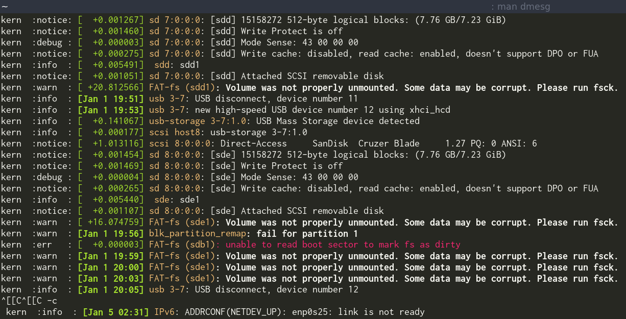
Figure 11: Screenshot of $\mathsf{dmesg}$

A.2.2 An $\omega$-RTE for $\mathsf{dmesg}$

We first give an $\omega$-RTE which analyzes the output of $\mathsf{dmesg}$, and produces the appropriate contexts. The RTE is a specification language which is easier to understand than the transducer which describes the same computation.

The required $\omega$-RTE inspects the output of $\mathsf{dmesg}$, and if it detects a line containing the message $\mathsf{err}$, then it outputs 10 lines before this line, 10 lines after this line as the necessary context needed to investigate the reason for the error. This is done for all lines containing $\mathsf{err}$.

The $\omega$-RTE is broken into two parts. We first look at the first 10 lines of the file. If any of these lines (say line $i$) has $\mathsf{err}$, we output the lines $1,\dots,i+10$.

1. Let $\backslash\mathsf{n}$ denotes newline, $\mathsf{char}=\Sigma\setminus\{\backslash\mathsf{n}\}$, $\mathsf{line}=\mathsf{char}^{+}\cdot\backslash\mathsf{n}$ and $\mathsf{err}_{i}=\mathsf{line}^{i}\cdot\mathsf{char}^{7}\cdot\mathsf{err}\cdot\Sigma^{\omega}$ be an expression which says that there is an “$\mathsf{err}$” in the $i+1$th line for $i\geq 0$. The message starts from the 8th character on each line, so we scan from the 8th character for $\mathsf{err}$.

2. Let $C_{i}$ = ${\mathsf{err}_{i}}\,?\,{[({\mathsf{line}^{i+11}}\,?\,{\mathsf{copy}}:{\bot})\mathbin{{\boxdot}}{(\mathsf{line}^{\omega}}\,?\,{\varepsilon}:{\bot})]}:{\varepsilon}$ be an $\omega$-RTE which gives the context of the error if the error is found in the $(i+1)$th line where $0\leq i\leq 9$. The RTE $\mathsf{copy}$ defines the identity function on $\Sigma^{+}$: For instance, if $\Sigma=\{a,b,c\}$ then $\mathsf{copy}={{a}\,?\,{a}:{({b}\,?\,{b}:{({c}\,?\,{c}:{\bot})})}}^{\scriptstyle{\boxplus}}$. Thus, if there is an “$\mathsf{err}$” in the first 10 lines, the context is generated using $C_{i}$.

3. To catch occurrences of “$\mathsf{err}$” in lines 11 and later in the file, we use $[\mathsf{line},C^{\prime}]^{21\omega}$, the 21-chained $\omega$-iteration. Here, $C^{\prime}$ is an RTE which copies the context for each line containing “$\mathsf{err}$” starting from line number 11:

   $$C^{\prime}={[\mathsf{line}^{10}\cdot\mathsf{char}^{7}\cdot\mathsf{err}\cdot\mathsf{char}^{+}\cdot\backslash\mathsf{n}\cdot\mathsf{line}^{10}]}\,?\,{\mathsf{copy}}:{\varepsilon}\,.$$

4. The required $\omega$-RTE $C$ = $C_{0}\odot C_{1}\odot\cdots\odot C_{9}\odot[\mathsf{line},C^{\prime}]^{21\omega}$.

Thus, the first 10 lines are checked for “$\mathsf{err}$” and the respective context is output if a line $0\leq i<10$ has “$\mathsf{err}$”; the remaining lines in the file are treated using the $[K,C^{\prime}]^{21\omega}$, where we look at blocks of 21 lines, and reproduce them as is, if the 11th line in the block has an “$\mathsf{err}$”; this is repeated from the next line and so on. The $[K,C^{\prime}]^{21\omega}$ is not a new combinator, it can be written in terms of 2-chained $\omega$-iteration as shown by Lemma A.1.

A.2.3 Machine description for $\mathsf{dmesg}$

Now we describe a transducer that produces the contexts based on the output of $\mathsf{dmesg}$. Since the $\mathsf{dmesg}$ command continuously monitors not only external devices, but also the RAM, processors, cache and the hard disk, the output is continuously updated in real time. Hence, the output is arbitrarily long.

The transducer ${\mathcal{A}}$ takes as input, the output as generated above, and needs the two way functionality. We do not use the look-ahead option here. Whenever ${\mathcal{A}}$ reads a line containing “$\mathsf{err}$”, it goes back 10 lines (or $i\leq 10$ lines, if there are only $i<10$ lines before the current line), and outputs the next 21 lines (or $11+i$ lines). Then it goes back 10 lines to check the message in the next line. The transducer ${\mathcal{A}}$ can be obtained inductively from the $\omega$-RTE $C$ described above, or it can be directly constructed. Because it has to count up to 10 several times, the automaton is rather large, but it can be constructed easily.

A.2.4 Reducing $k$-chained $\omega$-iteration to 2-chained $\omega$-iteration for $k>2$

Lemma A.1.

For $k>2$, the RTE $[L,f]^{k\omega}$ can be derived from RTEs defined in Section 3.2.

Proof A.2.

Let $L\subseteq\Sigma^{+}$ be a regular language, let $f\colon\Sigma^{+}\to\mathbb{D}$ and let $g=[L,f]^{k\omega}$. First, recall that by definition, $g(w)$ is defined as $f(u_{1}u_{2}\cdots u_{k})\cdot f(u_{2}u_{3}\cdots u_{k+1})\cdot f(u_{3}u_{4}\cdots u_{k+2})\cdots$ iff $w$ admits a unique factorization $w=u_{1}u_{2}u_{3}\cdots$ with each $u_{i}\in L$ for $i\geq 1$.

For $n>0$, we let $L_{n}$ be the set of words $w$ which admit a unique factorization $w=u_{1}u_{2}\cdots u_{n}$ with each $u_{i}\in L$ for $1\leq i\leq n$. Notice that $L_{n}\subseteq L^{n}\subseteq\Sigma^{+}$ is a regular language. We also define $L_{\omega}$ as the set of words $w\in\Sigma^{\omega}$ which admit a unique factorization $w=u_{1}u_{2}u_{3}\cdots$ with $u_{i}\in L$ for all $i\geq 1$. Indeed, $L_{\omega}\subseteq L^{\omega}$ is an $\omega$-regular language.

We define by induction for $n\geq 0$ a function $f_{n}$ such that $\mathsf{dom}(f_{n})\subseteq L_{k+n}$ and if $w=u_{1}u_{2}\cdots u_{k+n}$ is the unique factorization of $w$ with $u_{i}\in L$ for $1\leq i\leq k+n$ then

$$f_{n}(w)=f(u_{1}u_{2}\cdots u_{k})f(u_{2}u_{3}\cdots u_{k+1})\cdots f(u_{n+1}u_{n+2}\cdots u_{n+k})\,.$$

We let $f_{0}={L_{k}}\,?\,{f}:{\bot}$ and for $n>0$ we define $f_{n}=(f_{n-1}\mathbin{{\boxdot}}({L}\,?\,{\varepsilon}:{\bot}))\odot(({L_{n}}\,?\,{\varepsilon}:{\bot})\mathbin{{\boxdot}}f_{0})$. Note that this gives us $f_{1}=(f_{0}\mathbin{{\boxdot}}({L}\,?\,{\varepsilon}:{\bot}))\odot(({L}\,?\,{\varepsilon}:{\bot})\mathbin{{\boxdot}}f_{0})$, which works on strings of length $k+1$, and produces $f(u_{1}\cdots u_{k})f(u_{2}\cdots u_{k+1})$. Likewise, $f_{2}=(f_{1}\mathbin{{\boxdot}}({L}\,?\,{\varepsilon}:{\bot}))\odot(({L_{2}}\,?\,{\varepsilon}:{\bot})\mathbin{{\boxdot}}f_{0})$, which works on strings of length $k+2$, and produces $f_{1}(u_{1}\cdots u_{k+1})f(u_{3}\cdots u_{k+2})$, which in turn expands to $f(u_{1}\cdots u_{k})f(u_{2}\cdots u_{k+1})f(u_{3}\cdots u_{k+2})$.

Finally, let $h={L_{\omega}}\,?\,{[L_{k},f^{\prime}]^{2\omega}}:{\bot}$ with $f^{\prime}=f_{k-1}\mathbin{{\boxdot}}({L}\,?\,{\varepsilon}:{\bot})$. Notice that $\mathsf{dom}(f^{\prime})\subseteq L_{2k}$. We claim that $g(w)=h(w)$ for all $w\in\Sigma^{\omega}$.

Let $w\in L_{\omega}\supseteq\mathsf{dom}(g)\cup\mathsf{dom}(h)$. Consider the unique factorization $w=u_{1}u_{2}u_{3}\cdots$ with $u_{i}\in L$ for all $i\geq 1$. For all $i\geq 1$, let $w_{i}=u_{(i-1)k+1}\cdots u_{ik}$. Clearly, $w=w_{1}w_{2}w_{3}\cdots$ is the unique factorization of $w$ with $w_{i}\in L_{k}$ for all $i\geq 1$. Now, $h(w)=f^{\prime}(w_{1}w_{2})f^{\prime}(w_{2}w_{3})\cdots$ and for each $i\geq 1$ we have

$$f^{\prime}(w_{i}w_{i+1})=f(u_{(i-1)k+1}\cdots u_{ik})f(u_{(i-1)k+2}\cdots u_{ik+1})\cdots f(u_{ik}\cdots u_{ik+k-1})\,.$$

We deduce that $h(w)=g(w)$.

Example A.3.

Let $k=4$. We have $g=[L,f]^{4\omega}={L_{\omega}}\,?\,{[L_{4},f^{\prime}]^{2\omega}}:{\bot}$ by lemma A.1. We show the computation of $[L,f]^{4\omega}$ on a word $w\in L_{\omega}$ using this new RTE. Consider the unique factorization $w=u_{1}u_{2}u_{3}\cdots$ with $u_{i}\in L$ for all $i\geq 1$. Also, let $w_{1}=u_{1}\cdots u_{4}$, $w_{2}=u_{5}\cdots u_{8}$ and so on. We have $w_{i}\in L_{4}$ for all $i\geq 1$. Now,

$$[L,f]^{4\omega}(w)=f(u_{1}\cdots u_{4})f(u_{2}\cdots u_{5})\cdots\qquad\text{and}\qquad[L_{4},f^{\prime}]^{2\omega}(w)=f^{\prime}(u_{1}\cdots u_{8})f^{\prime}(u_{5}\cdots u_{12})\cdots$$

We show the expansion of $f^{\prime}(u_{1}\cdots u_{8})$ below.

$$f^{\prime}(u_{1}\cdots u_{8})$$

$$=(f_{3}\mathbin{{\boxdot}}({L}\,?\,{\varepsilon}:{\bot}))(u_{1}\cdots u_{8}) \text{def.\ of }f^{\prime}$$

$$=f_{3}(u_{1}\cdots u_{7})$$

$$=((f_{2}\mathbin{{\boxdot}}({L}\,?\,{\varepsilon}:{\bot}))\odot(({L_{3}}\,?\,{\varepsilon}:{\bot})\mathbin{{\boxdot}}f_{0}))(u_{1}\cdots u_{7}) \text{def.\ of }f_{3}$$

$$=f_{2}(u_{1}\cdots u_{6})\cdot f_{0}(u_{4}\cdots u_{7})$$

$$=((f_{1}\mathbin{{\boxdot}}({L}\,?\,{\varepsilon}:{\bot}))\odot(({L_{2}}\,?\,{\varepsilon}:{\bot})\mathbin{{\boxdot}}f_{0}))(u_{1}\cdots u_{6})\cdot f_{0}(u_{4}\cdots u_{7}) \text{def.\ of }f_{2}$$

$$=f_{1}(u_{1}\cdots u_{5})\cdot f_{0}(u_{3}\cdots u_{6})\cdot f_{0}(u_{4}\cdots u_{7})$$

$$=((f_{0}\mathbin{{\boxdot}}({L}\,?\,{\varepsilon}:{\bot}))\odot(({L}\,?\,{\varepsilon}:{\bot})\mathbin{{\boxdot}}f_{0}))(u_{1}\cdots u_{5})\cdot f_{0}(u_{3}\cdots u_{6})\cdot f_{0}(u_{4}\cdots u_{7}) \text{def.\ of }f_{1}$$

$$=f_{0}(u_{1}\cdots u_{4})\cdot f_{0}(u_{2}\cdots u_{5})\cdot f_{0}(u_{3}\cdots u_{6})\cdot f_{0}(u_{4}\cdots u_{7})$$

$$=f(u_{1}\cdots u_{4})\cdot f(u_{2}\cdots u_{5})\cdot f(u_{3}\cdots u_{6})\cdot f(u_{4}\cdots u_{7}) \text{def.\ of }f_{0}$$

Recursion tree for the same is shown in the figure 12. Hence,
$[L_{4},f^{\prime}]^{2\omega}(w)=f(u_{1}\cdots u_{4})\cdot f(u_{2}\cdots u_{5})\cdot f(u_{3}\cdots u_{6})\cdot f(u_{4}\cdots u_{7})\cdot f(u_{5}\cdots u_{8})\cdot f(u_{6}\cdots u_{9})\cdot f(u_{7}\cdots u_{10})\cdot f(u_{8}\cdots u_{11})\cdots$

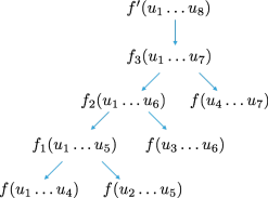
Figure 12: Computation of $f^{\prime}(u_{1}\cdots u_{8})$

Lemma A.4.

Similar to lemma A.1, the RTE $[L,f]^{k\scriptstyle{\boxplus}}$ can be derived from RTEs defined in Section 2.2 for $k>2$.

Proof A.5.

The proof technique is similar to Lemma A.1. Definitions of $L_{n},f_{n},f^{\prime}$ are as defined in this lemma. In addition we use $L_{+}$, the set of words having a unique decomposition $w=u_{1}u_{2}\cdots u_{n}$ with $n\geq 1$ and $u_{i}\in L$ for all $1\leq i\leq n$. We also use $L_{<k}=L_{0}\cup L_{1}\cup\cdots\cup L_{k-1}$, where $L_{0}=\{\varepsilon\}$. We define

$$h ={L_{+}}\,?\,{[\big{(}[L_{k},f^{\prime}]^{2\scriptstyle{\boxplus}}\mathbin{{\boxdot}}({L_{<k}}\,?\,{\varepsilon}:{\bot})\big{)}\odot\big{(}({L_{k}^{*}}\,?\,{\varepsilon}:{\bot})\mathbin{{\boxdot}}h^{\prime}\big{)}]}:{\bot}$$

$$h^{\prime} ={L_{k}}\,?\,{f}:{({L_{k+1}}\,?\,{f_{1}}:{({L_{k+2}}\,?\,{f_{2}}:{(\cdots({L_{2k-1}}\,?\,{f_{k-1}}:{\bot})\cdots)})})}\,.$$

We can show as in Lemma A.1 that $h=[L,f]^{k\scriptstyle{\boxplus}}$.

Appendix B Equivalence of Models

In this section, we look at the equivalence of the automata models for regular transformations on infinite words. The model used here is a two-way, deterministic Muller automaton, which has for each pair $(q,a)$ consisting of a state and symbol, a tuple of look-ahead $\omega$-regular languages which are mutually exclusive. The model (denoted 2WST_la) used in [4] however is a two-way deterministic Muller automaton which is equipped with a look-behind automaton (a NFA) and a look-ahead automaton (a possibly non-deterministic Muller automaton). Here, we show that these two models are equivalent in expressiveness.

Lemma B.1.

$\omega$-2DMT_la and 2WST_la (defined in [4]) are equivalent representations for $\omega-$regular transformations.

Proof B.2 (Proof sketch.).

• Given an $\omega$-2DMT_la ${\mathcal{A}}=(Q,\Sigma,\Gamma,q_{0},\delta,{\mathcal{F}},{\mathcal{R}})$, one can construct a 2WST_la ${\mathcal{A}}^{\prime}$ such that $[\![{\mathcal{A}}]\!]=[\![{\mathcal{A}}^{\prime}]\!]$. We create a look ahead automata $A_{L}$ as the disjoint union of all ${\mathcal{A}}_{i}=(Q_{i},\Sigma,s_{i},\delta_{i},{\mathcal{F}}_{i})$ corresponding to each look ahead language $R_{i}$ in ${\mathcal{R}}$: $\mathcal{L}({\mathcal{A}}_{i})=R_{i}$. The set of states of the 2WST_la ${\mathcal{A}}^{\prime}$ is $Q$, with initial state $q_{0}$ and Muller accepting set ${\mathcal{F}}$. The transition function $\delta^{\prime}$ of ${\mathcal{A}}^{\prime}$ is defined by $\delta^{\prime}(q,a,\Sigma^{*},{s_{i}})=(q^{\prime},\gamma,d)$, if $\delta(q,(a,R_{i}))=(q^{\prime},\gamma,d)$. Note that since we do not use any look-behind in ${\mathcal{A}}$, the look-behind automaton needed for the model in [4] is the trivial one which accepts all strings. Rather than writing the single state look-behind automaton (where the state is both accepting and initial), we write the expression $\Sigma^{*}$.

• Given 2WST_la ${\mathcal{T}}=((Q,\Sigma,\Gamma,\delta,q_{0},{\mathcal{F}}),{\mathcal{A}},{\mathcal{B}})$ with look-ahead automata ${\mathcal{A}}=(Q_{A},\Sigma,\delta_{A},{\mathcal{F}}_{A})$ and look-behind automata ${\mathcal{B}}=(Q_{B},\Sigma,\delta_{B},F_{B})$, one can construct an $\omega$-2DMT_la ${\mathcal{A}}^{\prime}=(Q^{\prime},\Sigma,\Gamma,q^{\prime}_{0},\delta^{\prime},{\mathcal{F}}^{\prime},{\mathcal{R}})$ such that $[\![{\mathcal{T}}]\!]=[\![{\mathcal{A}}^{\prime}]\!]$. For each state $p\in Q_{B}$ we let $K_{p}\subseteq\Sigma^{*}$ be the regular languages accepted by ${\mathcal{B}}$ with initial state $p$. Similarly, for each state $p\in Q_{A}$ we let $L_{p}\subseteq\Sigma^{\omega}$ be the $\omega$-regular languages accepted by ${\mathcal{A}}$ with initial state $p$. From the determinism of ${\mathcal{T}}$ we deduce that the languages $(K_{p})_{p\in Q_{B}}$ are mutually exclusive, and similarly the languages $(L_{p})_{p\in Q_{A}}$ are mutually exclusive.

  Now, a transition $\delta(q,(s_{B},a,s_{A}))=(q^{\prime},\gamma,d)$ of ${\mathcal{T}}$ can be replaced with the more abstract $\delta^{\prime}(q,(K_{s_{B}},a,L_{s_{A}}))=(q^{\prime},\gamma,d)$ using regular languages instead of states for look-ahead and look-behind. In order to obtain the $\omega$-2DMT_la it remains to remove the look-behind.

  Consider a DFA ${\mathcal{D}}=(Q_{D},\Sigma,\delta_{D},s_{D},(F_{p})_{p\in Q_{B}})$ which simultaneously recognizes all the $(K_{p})_{p\in Q_{B}}$: $K_{p}$ is the set of words accepted by ${\mathcal{D}}$ when using $F_{p}$ as set of final states. We define ${\mathcal{A}}^{\prime}$ as the synchronized product of ${\mathcal{T}}$ and ${\mathcal{D}}$. More precisely, we let $Q^{\prime}=Q\times Q_{D}$, $q^{\prime}_{0}=(q_{0},s_{D})$, ${\mathcal{R}}=\{L_{s_{A}}\mid s_{A}\in Q_{A}\}$, ${\mathcal{F}}^{\prime}$ consists of all $X\subseteq Q^{\prime}$ such that the projection of $X$ on $Q$ belongs to ${\mathcal{F}}$. The transition function $\delta^{\prime}$ is defined as follow. If $\delta(q,(s_{B},a,s_{A}))=(q^{\prime},\gamma,d)$ is a transition of ${\mathcal{T}}$, then $\delta^{\prime}((q,p),(a,L_{s_{A}}))=((q^{\prime},p^{\prime}),\gamma,d)$ is a transition of ${\mathcal{A}}^{\prime}$ provided

  • $p\in F_{s_{B}}$, i.e., the prefix read so far belongs to $K_{s_{B}}$, or equivalently, is recognized by the look-behind automaton ${\mathcal{B}}$ when starting from state $s_{B}$,

  • $p^{\prime}=\delta_{D}(p,a)$ if the transition moves forward ($d=+1$),

  • and if the transition moves backward ($d=-1$) then $p^{\prime}$ is obtained form $p$ using the reverse-run algorithm of Hopcroft and Ullman.

References

- [1] Rajeev Alur and Pavol Cerný. Expressiveness of streaming string transducers. In FSTTCS 2010, pages 1–12, 2010.
- [2] Rajeev Alur and Loris D’Antoni. Streaming tree transducers. J. ACM, 64(5):31:1–31:55, 2017.
- [3] Rajeev Alur, Loris D’Antoni, and Mukund Raghothaman. Drex: A declarative language for efficiently evaluating regular string transformations. In POPL 2015, pages 125–137, 2015.
- [4] Rajeev Alur, Emmanuel Filiot, and Ashutosh Trivedi. Regular transformations of infinite strings. In LICS 2012, pages 65–74, 2012.
- [5] Rajeev Alur, Adam Freilich, and Mukund Raghothaman. Regular combinators for string transformations. In LICS CSL-LICS ’14, pages 9:1–9:10, 2014.
- [6] Mikołaj Bojańczyk, Laure Daviaud, Bruno Guillon, and Vincent Penelle. Which classes of origin graphs are generated by transducers. In ICALP 2017, 2017.
- [7] Olivier Carton and Max Michel. Unambiguous büchi automata. Theoretical Computer Science, 297(1-3):37–81, Mar 2003.
- [8] Michal P. Chytil and Vojtěch Jákl. Serial composition of 2-way finite-state transducers and simple programs on strings. In ICALP 1977, pages 135–147, 1977.
- [9] Thomas Colcombet. Factorization forests for infinite words and applications to countable scattered linear orderings. Theoretical Computer Science, 411(4-5):751–764, Jan 2010.
- [10] Thomas Colcombet. The factorisation forest theorem. To appear in Handbook “Automata: from Mathematics to Applications”, 2013.
- [11] B. Courcelle. Handbook of graph grammars and computing by graph transformation. chapter The Expression of Graph Properties and Graph Transformations in Monadic Second-order Logic, pages 313–400. World Scientific Publishing Co., Inc., 1997.
- [12] Vrunda Dave, Shankara Narayanan Krishna, and Ashutosh Trivedi. Fo-definable transformations of infinite strings. In FSTTCS 2016, pages 12:1–12:14, 2016.
- [13] Manfred Droste, Werner Kuich, and Heiko Vogler. Handbook of Weighted Automata. Springer Publishing Company, 1st edition, 2009.
- [14] Joost Engelfriet and Hendrik Jan Hoogeboom. MSO definable string transductions and two-way finite state transducers. CoRR, cs.LO/9906007, 1999.
- [15] Emmanuel Filiot, Shankara Narayanan Krishna, and Ashutosh Trivedi. First-order definable string transformations. In FSTTCS 2014, pages 147–159, 2014.
- [16] Paul Gastin and Shankara Narayanan Krishna. Unambiguous forest factorization. Unpublished.
- [17] Imre Simon. Factorization forests of finite height. Theoretical Computer Science, 72(1):65–94, Apr 1990.
- [18] Thomas Wilke. Backward deterministic buüchi automata on infinite words. In FSTTCS 2017, pages 6:1–6:10, 20147. To appear.