ZH-TH 06/18

Diphoton production at the LHC:
a QCD study up to NNLO

Stefano Catani${}^{(a)},$ Leandro Cieri${}^{(b,c)},$ Daniel de Florian^(d),
Giancarlo Ferrera^(e) and Massimiliano Grazzini^(c)

^(a) INFN, Sezione di Firenze and Dipartimento di Fisica e Astronomia,

Università di Firenze, I-50019 Sesto Fiorentino, Florence, Italy

^(b) INFN, Sezione di Milano-Bicocca,

Piazza della Scienza 3, I-20126 Milano, Italy

^(c) Physik-Institut, Universität Zürich, CH-8057 Zurich, Switzerland

^(d) International Center for Advanced Studies (ICAS), ECyT-UNSAM,

Campus Miguelete, 25 de Mayo y Francia, (1650) Buenos Aires, Argentina

^(e) Dipartimento di Fisica, Università di Milano and

INFN, Sezione di Milano, I-20133 Milan, Italy

Abstract

We consider the production of prompt-photon pairs at the LHC and we report on a study of QCD radiative corrections up to the next-to-next-to-leading order (NNLO). We present a detailed comparison of next-to-leading order (NLO) results obtained within the standard and smooth cone isolation criteria, by studying the dependence on the isolation parameters. We highlight the role of different partonic subprocesses within the two isolation criteria, and we show that they produce large radiative corrections for both criteria. Smooth cone isolation is a consistent procedure to compute QCD radiative corrections at NLO and beyond. If photon isolation is sufficiently tight, we show that the NLO results for the two isolation procedures are consistent with each other within their perturbative uncertainties. We then extend our study to NNLO by using smooth cone isolation. We discuss the impact of the NNLO corrections and the corresponding perturbative uncertainties for both fiducial cross sections and distributions, and we comment on the comparison with some LHC data. Throughout our study we remark on the main features that are produced by the kinematical selection cuts that are applied to the photons. In particular, we examine soft-gluon singularities that appear in the perturbative computations of the invariant mass distribution of the photon pair, the transverse-momentum spectra of the photons, and the fiducial cross section with asymmetric and symmetric photon transverse-momentum cuts, and we present their behaviour in analytic form.

February 2018

1 Introduction

The production of photon pairs (diphotons) with high invariant mass at high-energy hadron colliders is a very relevant process in the context of both Standard Model (SM) studies and searches for new-physics signals.

Experimentally a pair of photons is a very clean final state, and photon energies and momenta can be measured with high precision in modern electromagnetic calorimeters. Since photons do not interact strongly with other final-state particles, prompt photons represent ideal probes to test the properties of the SM and corresponding theoretical predictions (see Refs. [1]–[8] for recent experimental analyses of Tevatron and LHC diphoton data). Measurements involving a pair of isolated photons have played a crucial role in the discovery at the LHC [9, 10] of a Higgs boson, whose properties are compatible with those of the SM one. Studies of the Higgs boson properties in the diphoton decay mode have been performed [11, 12]. Diphoton measurements (see, e.g., Refs. [13]–[18]) are also important in many new-physics scenarios, including searches for extra dimensions or supersymmetry. The relevance of LHC measurements of the diphoton invariant-mass spectrum is highlighted by the recent observation [19]–[23] of an excess of events with invariant mass of about 750 GeV that might have indicated the presence of resonances over the diphoton SM background. That observation raised a great deal of attention from December 2015 till the time of the 2016 Summer Conferences [24, 25].

Owing to its physics relevance, the study of diphoton production requires accurate theoretical calculations which, in particular, include QCD radiative corrections at high perturbative orders. In high-energy collisions, final-state prompt photons with high transverse momentum can be originated through direct production from hard-scattering subprocesses and through fragmentation subprocesses of QCD partons. The theoretical computation of fragmentation subprocesses requires non-perturbative information, in the form of parton fragmentation functions of the photon, which typically has large associated uncertainties. However, the effect of fragmentation contributions is significantly reduced by the photon isolation criteria that are necessarily applied in hadron collider experiments to suppress the very large reducible background of ‘non-prompt’ photons (e.g., photons that are faked by jets or produced by hadron decays). Two such criteria are the so-called ‘standard’ cone isolation and the ‘smooth’ cone isolation proposed by Frixione [26]. The standard cone isolation is the criterion that is typically used by experimental analyses. This criterion can be experimentally implemented in a relatively straightforward manner, but it only suppresses part of the fragmentation contribution. By contrast, the smooth cone isolation (formally) eliminates the entire fragmentation contribution, although, due to the finite granularity of the detectors, it cannot be directly applied at the experimental level in its original form. Owing to the absence of fragmentation contributions, theoretical calculations are much simplified by using the smooth cone isolation, and it is relatively simpler to compute radiative corrections at high perturbative orders. Considering calculations at the next-to-leading order (NLO) in the QCD coupling $\alpha_{S}$, in Ref. [27] it was shown that, if the isolation is ‘tight enough’, the two isolation criteria lead to theoretical NLO results that are quantitatively very similar for various observables in diphoton production processes at high-energy hadron colliders.

In the present paper we deal with the diphoton production process $pp\rightarrow\gamma\gamma X$, where $p$ is a colliding proton and $X$ denotes the inclusive final state that accompanies the $\gamma\gamma$ pair. QCD radiative corrections to this process were first computed up to the NLO in Ref. [28]. This is a complete NLO calculation of both the direct and fragmentation (specifically, single- and double-fragmentation) components of the cross section. The calculation is implemented at the fully-differential level in the numerical Monte Carlo code DIPHOX, which can be used to perform computations with any infrared and collinear safe isolation criteria (including the standard and smooth cone criteria). The DIPHOX calculation also includes the so-called box contribution [29] to the partonic channel $gg\rightarrow\gamma\gamma$ (which is formally a contribution of next-to-next-to-leading order (NNLO) type), since this contribution can be quantitatively enhanced by the large gluon–gluon parton luminosity at high-energy hadron–hadron colliders. The next-order gluonic corrections to the box contribution (which are part of the N³LO QCD corrections to diphoton production) were computed in Ref. [30] (and implemented in the numerical program GAMMA2MC) and found to have a moderate quantitative effect. An independent NLO calculation [31] is implemented in the code MCFM, which, however, includes the fragmentation component only at the leading order (LO), while the box contribution is treated according to the GAMMA2MC code. A complete calculation at the NNLO of both the direct and fragmentation components still nowadays remains computationally very challenging.

Fragmentation contributions are absent by considering smooth cone isolation. In the context of smooth cone isolation, diphoton production at the LO (i.e. at $\mathcal{O}(\alpha_{S}^{0})$) emerges via the quark–antiquark annihilation subprocess $q\bar{q}\rightarrow\gamma\gamma$. The NLO QCD corrections are due to quark–antiquark annihilation and to new partonic channels (via the subprocess $qg\rightarrow\gamma\gamma q$ and ${\bar{q}}g\rightarrow\gamma\gamma{\bar{q}}$) with an initial-state colliding gluon. At the NNLO the $gg$ channel starts to contribute and it (the entire channel and not only its box contribution) can be fully consistently included in the perturbative QCD calculation. The large value of the gluon parton distribution function (PDF) of the colliding proton makes the gluon initiated channels important, especially at small and intermediate values of the diphoton invariant mass. The scattering amplitudes that are needed to evaluate the NNLO QCD corrections were computed in Ref. [29, 32, 33, 34], and they were used in Ref. [35] to perform the first NNLO calculation of diphoton production in hadronic collisions. The NNLO calculation at the fully-differential level is based on the $q_{T}$ subtraction method [36] and it was implemented [35] in the numerical code 2$\gamma$NNLO. More recently, an independent calculation of diphoton production at the NNLO has been performed in Ref. [37] by using the method of $N$-jettiness subtraction [38, 39]. The NNLO calculation of Ref. [37] is implemented [40] in the MCFM program. An independent NNLO computation of diphoton production at the NNLO, based on the $q_{T}$ subtraction method, has been implemented in the general purpose NNLO generator MATRIX [41].

The transverse-momentum spectrum of the photon pair is sensitive to logarithmically-enhanced contributions at high perturbative orders. Transverse-momentum resummation at next-to-next-to-leading logarithmic (NNLL) accuracy for inclusive diphoton production was implemented [42] in the ResBos code, and more recently the complete NNLL calculation has been combined with the NNLO contributions and implemented in the numerical program 2$\gamma$Res [43].

Using smooth cone isolation, associated production of diphotons and jets has been computed up to NLO for various jet multiplicities, namely, $\gamma\gamma+1$ jet [44, 45] (the fragmentation component at LO is included in the calculations of Refs. [45, 46]), $\gamma\gamma+2$ jets [47, 48, 49], $\gamma\gamma+2~{}\!b$-jets [50] and $\gamma\gamma+3$ jets [49]. Owing to the computational simplifications of smooth cone isolation (with respect to standard cone isolation), some hadron collider processes with one final-state photon, such as associated $Z\gamma$ [51, 52, 53] and $W\gamma$ [52] production and inclusive single-photon production [54], have also been computed up to the NNLO in QCD perturbation theory.

Lowest-order electroweak radiative corrections to diphoton production at LHC energies have been computed in Refs. [55, 56]. They produce small effects on NNLO QCD results for inclusive diphoton production. The effects can increase by selecting photons with transverse momenta in the TeV region.

In this paper we present studies of NLO and NNLO QCD radiative corrections to inclusive diphoton production at LHC energies. The results at the NNLO are based on the theoretical calculation of Ref. [35], as implemented in the fully-differential Monte Carlo program 2$\gamma$NNLO, and on the independent NNLO calculation implemented in MATRIX [41]. The first version of 2$\gamma$NNLO, which was originally used in Ref. [35], had a numerical implementation bug that was subsequently corrected. A main result of Ref. [35] is that NNLO radiative corrections are substantial for diphoton kinematical configurations of interest at high-energy hadron colliders. The selected quantitative results that were presented in Ref. [35] are mostly related to diphoton kinematical configurations that are typically examined in Higgs boson searches and studies at the LHC. In this paper we consider more general kinematical configurations. In particular, we present NLO and NNLO studies related to photon isolation, and we discuss various detailed features of the theoretical results up to NNLO.

The results of the code 2$\gamma$NNLO have been used by experimental collaborations in some of their data/theory comparisons. The analyses performed at the Tevatron ($\sqrt{s}=1.96$ TeV) by the CDF [5] and D0 [6] collaborations and at the LHC ($\sqrt{s}=7$ TeV and 8 TeV) by the ATLAS [4, 8] and CMS [7] collaborations show that the inclusion of the NNLO corrections greatly improves the description of diphoton production data. The NNLO predictions have also been used in data analyses related to new-physics searches in high-mass diphoton events at $\sqrt{s}=13$ GeV [20]. In summary, these measurements prove that the NNLO results are important to understand phenomenological aspects of diphoton production.

The paper is organized as follows. Section 2 is devoted to a comprehensive study of photon isolation. In particular, we perform a detailed comparison of the standard and smooth isolation criteria in the context of perturbative QCD results at LO and NLO. We discuss the role of different partonic subprocesses within the two different isolation criteria. We also remark on the effects that are produced by the isolation parameters and by the kinematical selection cuts that are applied to the photons. Specifically, in Sect. 2.1 we introduce the photon isolation criteria and comment on some of their features. The QCD calculations that are used in our study are briefly described in Sect. 2.2. The quantitative results for total and differential cross sections are presented in Sect. 2.3. Section 2.3.1 is devoted to the LO and NLO results for total cross sections. Results for differential cross sections at LO and NLO are presented in Sects. 2.3.2 and 2.3.3, respectively. In Sect. 3 we present detailed NNLO results for diphoton production within the smooth isolation prescription. We study the perturbative stability of the results and we discuss related theoretical uncertainties by considering several observables that are relevant in diphoton production at hadronic colliders. We also discuss the comparison of the NNLO predictions to recent LHC data [4]. Specifically, results for total cross sections and differential cross sections are presented in Sects. 3.1 and 3.2, respectively. In Sect. 3.3 we present some results on the dependence on the isolation parameters. The comparison with LHC data is discussed in Sect. 3.4. In Sect. 3.5 we discuss the effects of (asymmetric and symmetric) photon transverse-momentum cuts on total and differential cross sections and, in particular, we comment on related perturbative (soft-gluon) instabilities. Finally, in Sect. 4 we summarize our results.

2 Photon isolation

2.1 Isolation criteria

Hadron collider experiments at the Tevatron and the LHC do not perform inclusive photon measurements. The background of secondary photons coming from the decays of $\pi^{0}$, $\eta$, etc. overwhelms the signal by several orders of magnitude and the experimental selection of prompt diphotons requires isolation cuts (or criteria) to reject this background. The standard cone isolation and the smooth cone isolation are two of these criteria. Both criteria consider the amount of hadronic (partonic) transverse energy $E_{T}^{had}(r)=\sum_{i}E_{T\,i}^{had}\;\Theta(r-R_{i\gamma})$ inside a cone of radius $r$ around the direction of the photon momentum ${\bf p}_{\gamma}$. Then the isolated photons are selected by limiting the value of $E_{T}^{had}(r)$.

The standard cone isolation criterion fixes the size $R$ of the radius of the isolation cone and it requires

$$E_{T}^{had}(R)\leq\,E_{T\,{\rm max}}\;\;,$$ (1)

where the isolation parameter $E_{T\,{\rm max}}$ can be either a fixed value of transverse energy or a function of the photon transverse momentum $p_{T\gamma}$ (i.e., $E_{T\,{\rm max}}=\epsilon\,p_{T\gamma}$ with a fixed parameter $\epsilon$). A combination of these two options is also possible: for instance, $E_{T\,{\rm max}}=0.05\,p_{T\gamma}+6$ GeV is used in the study of Refs. [19, 22].

Provided $E_{T\,{\rm max}}$ is finite (not vanishing) standard cone isolation leads to infrared-safe cross sections [57] in QCD perturbation theory. Parton radiation exactly collinear with the direction of the photon momentum is allowed by the constraint in Eq. (1) and, as a consequence, the treatment of standard cone isolation within perturbative QCD requires the introduction of parton to photon fragmentation functions. Decreasing the value of $E_{T\,{\rm max}}$ reduces and suppresses the effect of the fragmentation function (and of the corresponding partonic subprocesses).

The smooth cone isolation criterion [26] (see also Refs. [58, 59]) also fixes the size $R$ of the isolation cone and it requires

$$E_{T}^{had}(r)\leq\,E_{T\,{\rm max}}~{}\chi(r;R)\;,\quad\mbox{ in {\it all} cones with}\;r\leq R\;\;,$$ (2)

with a suitable choice of the $r$ dependence of the isolation function $\chi(r;R)$. The two key properties [26] of the isolation function are: $\chi(r;R)$ has to smoothly vanish as the cone radius $r$ vanishes ($\chi(r)\rightarrow 0\;,\;\mbox{if}\;\;r\rightarrow 0\,$), and it has to fulfil the condition $\;0<\chi(r;R)\leq 1$ (in particular, $\chi$ must not vanish) for any finite (non-vanishing) value of $r$. Since $E_{T}^{had}(r)$ does not increase by decreasing $r$, in practice the requirement in Eq. (2) is effective only if $\chi(r;R)$ monotonically decreases as $r$ decreases.

The smooth cone isolation criterion implies that, closer to the photon, less hadronic activity is allowed. The amount of energy deposited by parton radiation at angular distance $r=0$ from the photon is required to be exactly equal to zero, and the fragmentation component (which has a purely collinear origin in perturbative QCD) of the cross section vanishes completely. The cancellation of perturbative QCD soft divergences still takes place as in ordinary infrared-safe cross sections, since parton radiation is not forbidden in any finite region of the phase space [26]. It is also preferable to choose isolation functions $\chi(r;R)$ with a sufficiently smooth dependence on $r$ over the entire range $0<r<R$. In particular, large discontinuities of $\chi(r;R)$ at finite values of $r$ are potential sources of instabilities [60] in fixed-order perturbative calculations. Small discontinuities of the function $\chi(r;R)$ (such as those in the discretized version [61] of smooth cone isolation) are instead acceptable.

A customary choice of the isolation function $\chi(r;R)$ is

$$\chi(r;R)=\left(\frac{1-\cos(r)}{1-\cos(R)}\right)^{n}\;,$$ (3)

where the value of the power $n$ is typically set to $n=1$. We also consider the following isolation function:

$$\chi(r;R)=\left(\frac{r}{R}\right)^{2n}\;,$$ (4)

whose value depends on the ratio $r/R$ (rather than $r$ and $R$, independently). The two functions in Eqs. (3) and (4) are equal at the isolation cone boundary $r\rightarrow R$ ($\chi(r;R)\rightarrow 1$) and they behave similarly as $r\rightarrow 0$ ($\chi(r;R)\propto r^{2n}$).

Comparing the isolation requirements in Eqs. (1) and (2) by using the same values of $R$ and $E_{T\,{\rm max}}$ in both equations, we see that smooth cone isolation is more restrictive than standard cone isolation. Therefore, the following physical constraint applies:

$$d\sigma_{\rm smooth}(R;E_{T\,{\rm max}})<d\sigma_{\rm standard}(R;E_{T\,{\rm max}})\;\;,$$ (5)

where $d\sigma$ generically denotes total cross sections and differential cross sections with respect to photon kinematical variables, and the subscripts ‘smooth’ and ‘standard’ refer to smooth and standard isolation, respectively. Note that the isolation parameters $R$ and $E_{T\,{\rm max}}$ are set at the same values in the two isolated cross sections, $d\sigma_{\rm smooth}$ and $d\sigma_{\rm standard}$, that are compared in the inequality (5) (e.g., the inequality is not necessarily valid if smooth isolation at a given value of $E_{T\,{\rm max}}$ is compared with standard isolation at a different and smaller value of $E_{T\,{\rm max}}$). An analogous reasoning applies to the cross section dependence on the isolation parameters $E_{T\,{\rm max}}$ and $R$, since the isolation requirement can become more or less restrictive by varying these parameters. Therefore, we have the following physical behaviour:

$$d\sigma_{\rm is}(R;E_{T\,{\rm max}})\;\;\mbox{monotonically decreases as}~{}E_{T\,{\rm max}}~{}\mbox{decreases}\;\;(R~{}\mbox{fixed})\;\;,$$ (6)

$$d\sigma_{\rm is}(R;E_{T\,{\rm max}})\;\;\mbox{monotonically increases as}~{}R~{}\mbox{decreases}\;\;(E_{T\,{\rm max}}~{}\mbox{fixed})\;\;,$$ (7)

$$d\sigma_{\rm smooth}(R;E_{T\,{\rm max}};n)\;\;\mbox{monotonically decreases as}~{}n~{}\mbox{increases}\;\;(R~{}\mbox{and}~{}E_{T\,{\rm max}}~{}\mbox{fixed})\;\;,$$ (8)

and the subscript ‘is’ equally applies to both isolation criteria (e.g., ‘is’=‘smooth’ or ‘is’=‘standard’). The relation (8) refers to the dependence on the power $n$ in the case of the isolation function in Eqs. (3) or (4) (a similar relation applies to the cross section dependence by considering two isolation functions $\chi_{1}(r)$ and $\chi_{2}(r)$ such that $\chi_{1}(r)>\chi_{2}(r)$).

The standard cone isolation criterion is simpler and, as stated in the Introduction, it is the criterion that is used in experimental analyses at hadron colliders (the actual experimental selection of isolated photons, including isolation requirements, is definitely much more involved than the relatively straightforward implementation of the criterion). The experimental implementation of smooth cone isolation (in its strict original form) is complicated especially by the finite granularity of the Tevatron and LHC detectors.

Independently of the intrinsic differences between the standard and smooth cone isolation criteria, Eq. (5) implies that a reliable (theoretical or experimental) cross section result with smooth cone isolation represents a lower bound on the corresponding (i.e., with the same values of $E_{T\,{\rm max}}$ and $R$) cross section result with standard cone isolation (this statement is valid within reliable estimates of related theoretical or experimental uncertainties). In particular, this also implies that a comparison between theoretical smooth isolation results and experimental standard isolation results leads to meaningful and valuable information.

The comparison between smooth and standard isolation can be sharpened by considering tight isolation requirements. As expected on general grounds, the differences between the two isolation criteria should be reduced in the case of tight isolation cuts. This expectation is confirmed by the diphoton studies in Refs. [27, 67], which show theoretical NLO results that are similar for the two isolation criteria if the isolation parameters are tight enough (e.g., $R=0.4$ and $E_{T\,{\rm max}}<5~{}$GeV or $E_{T\,{\rm max}}=\epsilon\,p_{T\gamma}$ with $\epsilon<0.1$ as in Sect. 11 of Ref. [27] or Sect. 4.3.1 of Ref. [67]).

In Sect. 2.3 we present detailed results for smooth and standard isolation. We study the dependence on the isolation parameter $E_{T\,{\rm max}}$ and its effects on both total cross sections and differential cross sections in various kinematical regions.

2.2 Perturbative QCD calculations

In this paper we present quantitative results on QCD radiative corrections to diphoton production by using both smooth cone and standard cone isolations. We consider total cross sections (more precisely, fiducial cross sections) and differential cross sections as functions of various kinematical variables of the prompt photons. The kinematical variables that we use are the diphoton invariant mass $M_{\gamma\gamma}$, the photon polar angle $\theta^{*}$ in the Collins–Soper rest frame [68] of the diphoton system, the azimuthal angle separation $\Delta\Phi_{\gamma\gamma}$ between the two photons, the diphoton transverse momentum $p_{T\gamma\gamma}$ and the transverse momenta $p_{T\gamma}^{hard}$ and $p_{T\gamma}^{soft}$ ($p_{T\gamma}^{hard}>p_{T\gamma}^{soft}$) of the harder and softer photon of the diphoton pair. As previously specified, azimuthal angles and transverse momenta are defined in the centre–of–mass frame of the colliding hadrons.

The QCD results on smooth cone isolation are obtained by using the numerical programs 2$\gamma$NNLO [35] and MATRIX [41], which include perturbative QCD contributions up to NNLO. The NNLO calculations are based on the $q_{T}$ subtraction method [36], which is applicable to hadroproduction processes of generic high-mass systems of colourless particles and it has been already applied to explicit NNLO calculations of several specific processes (Higgs boson [36, 69] and vector boson [70, 71] production, associated production of a Higgs boson and a vector boson [72, 73], diboson production processes such as $Z\gamma$ [51, 52], $W^{\pm}\gamma$ [52], $ZZ$ [74, 75], $W^{+}W^{-}$ [76, 77] and $W^{\pm}Z$ [78] production, Higgs boson pair production [79], associated production of a Higgs boson pair and a $W$ or a $Z$ boson [80]). The $q_{T}$ subtraction method has recently been extended to heavy-quark production and applied to the NNLO calculation of top quark pair production [81].

In the case of diphoton production, the method combines the NLO cross section $d\sigma_{\gamma\gamma+{\rm jets}}$ for the production of the photon pair plus one or two jets (partons) with an appropriate subtraction counterterm (its explicit expression is given in Ref. [82]) and a hard-virtual contribution (see Ref. [83]) for diphoton production with no additional final-state jets (partons). In the code 2$\gamma$NNLO the cross section $d\sigma_{\gamma\gamma+{\rm jets}}$ is computed up to NLO by using the dipole-subtraction method [84] as implemented in the diphoton calculation of Ref. [44]. In MATRIX the cross section $d\sigma_{\gamma\gamma+{\rm jets}}$ is computed at NLO by using the fully automated implementation of the dipole-subtraction method within the Monte Carlo program MUNICH, and all (spin- and colour-correlated) tree-level and one-loop amplitudes are obtained from OpenLoops [85]. The combination of $d\sigma_{\gamma\gamma+{\rm jets}}$ and its counterterm is numerically finite, although the two contributions are separately divergent in the limit of vanishing transverse momentum $p_{T\gamma\gamma}$ of the photon pair. In 2$\gamma$NNLO the cancellation of the separate divergences is numerically treated by introducing a lower limit $q_{T\rm cut}$ on $p_{T\gamma\gamma}$ ($p_{T\gamma\gamma}>q_{T\rm cut}$) and considering small values of $q_{T\rm cut}$ (formally performing the limit $q_{T\rm cut}\rightarrow 0$). Decreasing the value of $q_{T\rm cut}$ reduces the size of systematical errors (due to the finite value of $q_{T\rm cut}$) at the expense of increasing computational time and resources to handle numerical instabilities. As a practical compromise, in our study we use a finite value of $q_{T\rm cut}$ in the range $q_{T\rm cut}=0.1$ GeV–0.2 GeV. The NNLO generator MATRIX implements instead a lower limit $r_{\rm cut}$ on the ratio $p_{T\gamma\gamma}/M_{\gamma\gamma}$ ($p_{T\gamma\gamma}>r_{\rm cut}M_{\gamma\gamma}$) [41], and we use values in the range $r_{\rm cut}=0.08\%$–$0.15\%$.

Owing to the finite values of $q_{T\rm cut}$ or $r_{\rm cut}$, a systematical uncertainty of about $\pm{\cal O}(1\%)$ affects all the NNLO results presented in this paper. The quoted systematical uncertainty is sufficient for the purpose of the studies that we present throughout the paper. It is substantially smaller than the size of additional (NLO) NNLO theoretical uncertainties that we find, for instance, by performing customary variations of the factorization and renormalization scales at (NLO) NNLO. We also note that, at fixed value of $q_{T\rm cut}$ ($r_{\rm cut}$), the NNLO systematical error on differential cross sections tends to be larger than the corresponding error on total cross sections. In particular, some specific observables (and, more precisely, their value in restricted kinematical regions) that are very sensitive to the detailed shape of the $p_{T\gamma\gamma}$ distribution in the limit $p_{T\gamma\gamma}\rightarrow 0$ can be affected by larger NNLO systematical errors due to the finite value of $q_{T\rm cut}$ ($r_{\rm cut}$): these observables may require refined numerical studies with smaller values of $q_{T\rm cut}$ ($r_{\rm cut}$). Nonetheless, these same specific observables are (expected to be) affected by increased theoretical uncertainties due to large higher-order perturbative corrections (instabilities). Examples of these observables are the differential cross section $d\sigma/d\Delta\Phi_{\gamma\gamma}$ at $\Delta\Phi_{\gamma\gamma}\simeq\pi$, and the differential cross sections $d\sigma/dM_{\gamma\gamma}$, $d\sigma/dp_{T\gamma}^{hard}$ and $d\sigma/dp_{T\gamma}^{soft}$ (or related integrated quantities) in soft-gluon sensitive kinematical regions (see Sect. 3.5).

We use 2$\gamma$NNLO and MATRIX to obtain results at LO, NLO and NNLO in QCD perturbation theory. At each order our calculation includes all the terms (and only those terms) that contribute to the total cross section at the corresponding perturbative order according to the formal expansion in powers of $\alpha_{S}$. Therefore (in the context of smooth cone isolation), only the initial-state $q{\bar{q}}$ partonic channel contributes at LO, the initial-state $qg$ and ${\bar{q}}g$ channels start to contribute at NLO, and the initial-state $gg$ channel starts to contribute at NNLO. In particular the box contribution $gg\rightarrow\gamma\gamma$ [29] only enters at NNLO, together with all the partonic subprocesses (e.g., including the gluon initiated subprocess $gg\rightarrow\gamma\gamma q{\bar{q}}$) that contribute at the same order. We do not include the NLO correction [30] to the box contribution, since it is part of the complete (and still unknown) N³LO corrections to inclusive diphoton production. All the partonic subprocesses are treated in the massless-quark framework with $N_{f}=5$ quark flavours. In particular, we do not include NNLO contributions with virtual top quarks since they are not yet fully known (e.g., the loop top quark contribution to the two-loop scattering amplitude $q{\bar{q}}\rightarrow\gamma\gamma$ has not yet been computed in complete form [86]). The effect of including the NLO correction [30] and the top quark correction to the (massless-quark) box contribution $gg\rightarrow\gamma\gamma$ has been considered in the diphoton calculation of Ref. [37]. The top quark correction to the box contribution is also studied in Refs. [87] and [88].

The results on standard cone isolation are obtained by using the DIPHOX calculation [28], which includes QCD radiative corrections up to the NLO. The NLO calculation that is implemented in DIPHOX is based on a combined use [28, 89] of the subtraction and phase-space slicing methods. The slicing approximation is applied [28] to the phase-space region where the minimum transverse-momentum of the three final-state partons at NLO is smaller than $p_{Tm}$ (formally considering the limit $p_{Tm}\rightarrow 0$). Our numerical results are obtained by using $p_{Tm}=0.1$ GeV, which is the default value of the slicing parameter (regulator) $p_{Tm}$ that is suggested in the DIPHOX program. Since we are interested in an order-by-order comparison with smooth cone isolation results, the box contribution $gg\rightarrow\gamma\gamma$ is not included in the DIPHOX NLO results. Note, however, that at LO and NLO all the initial-state partonic channels ($q{\bar{q}},qg,{\bar{q}}g,gg$) contribute in DIPHOX because of the presence of a non-vanishing fragmentation component (though the fragmentation component is quantitatively suppressed by the isolation procedure). Owing to the double-fragmentation component, even the initial-state $gg$ channel is not vanishing at LO (at NLO the initial-state $gg$ channel contributes also through the single-fragmentation component).

We note that (due to the limited number of final-state partons in fixed-order computations) LO calculations do not cover the entire kinematical region for inclusive diphoton production. LO calculations give non-vanishing cross sections only in limited LO kinematical subregions. Outside these subregions, only the NLO results start to give non-vanishing cross section contributions. Therefore, outside the LO kinematical subregions the NLO (NNLO) results effectively represent an LO (NLO) perturbative QCD prediction. In spite of the effective meaning of the results, we always use the default labels LO, NLO and NNLO according to the perturbative order in which the results contribute to the inclusive (total) cross section. For example, in the case of the $\Delta\Phi_{\gamma\gamma}$ distribution, the LO kinematical subregion has $\Delta\Phi_{\gamma\gamma}=\pi$: the region of small values of $\Delta\Phi_{\gamma\gamma}$ receives contributions only from the NLO and NNLO results that represent effective LO and NLO predictions, respectively. We also note that the LO kinematical subregions can be different in the context of smooth cone and standard cone isolation. For instance, at LO $p_{T\gamma\gamma}=0$ and $p_{T\gamma}^{hard}=p_{T\gamma}^{soft}$ in the case of smooth cone isolation, whereas $p_{T\gamma\gamma}$ can be different from zero and $p_{T\gamma}^{hard}\geq p_{T\gamma}^{soft}\geq p_{T\gamma}^{hard}-E_{T\,{\rm max}}$ in the case of standard cone isolation (non-vanishing values of $p_{T\gamma\gamma}$ are produced through the LO fragmentation component of the cross section). We also comment about the dependence on the isolation parameters $R$ and $E_{T\,{\rm max}}$ (the comment has similarities with our previous comment on LO kinematical subregions). The LO results are independent of the size $R$ of the isolation cone. The LO cross section depends on $E_{T\,{\rm max}}$ in the case of standard cone isolation (the $E_{T\,{\rm max}}$ dependence is due to the fragmentation component), while it is independent of the value of $E_{T\,{\rm max}}$ in the case of smooth cone isolation.

In Eqs. (5)–(8) we have listed some constraints on isolated photon cross sections. These are physical constraints (properties) in the sense that they apply to physical (‘positive definite’) events: if the isolation requirements are more (less) restrictive, the selected number of isolated photons decreases (increases). Such properties do not ‘a priori’ apply to theoretical calculations based on perturbative QCD (of course, if the constraints are not fulfilled, the perturbative QCD calculation is not a reliable approximation of the physical result) since, beyond the effective LO approximation, they involve negative-weight contributions (which are due to virtual radiative corrections and to subtraction contributions related to the factorization procedure of parton distribution functions and fragmentation functions).

As is well known, fixed-order perturbative results can show unphysical behaviour in specific kinematical regions. In the case of diphoton production, for instance, it is known [28] that the differential cross sections at small values of $p_{T\gamma\gamma}$ ($p_{T\gamma\gamma}\rightarrow 0$) or large values of $\Delta\Phi_{\gamma\gamma}$ ($\Delta\Phi_{\gamma\gamma}\rightarrow\pi$) cannot be reliably computed in fixed-order perturbation theory: the disease is due to large logarithmic corrections that have to be resummed to all perturbative orders [42, 43] to recover the physical behaviour and predictivity.

In the presence of photon isolation cuts, perturbative computations of total cross sections can also show some misbehaviour. Isolated (with both smooth and standard isolation) photon cross sections fulfil the physical constraint $\sigma_{\rm is}(R;E_{T\,{\rm max}})<\sigma_{\rm inc}$, where $\sigma_{\rm inc}$ is the inclusive (non-isolated) cross section. Nonetheless, in the case of standard cone isolation at NLO this constraint is violated [57] at very small values ($R\raisebox{-2.58334pt}{\hbox to0.0pt{$\,\sim\,$\hss}}\raisebox{1.72218pt}{$\,<\,$}0.1$) of the radius $R$ of the isolation cone. The violation is due to large logarithmic ($\ln R$) corrections, and the physical behaviour is recovered through a corresponding all-order resummation procedure [90]. We expect a (qualitatively) similar $\ln R$ dependence in the case of smooth cone isolation, though in the present paper we do not consider very small values of $R$.

Violation of expected properties is not necessarily related to logarithmically-enhanced QCD corrections: it can be simply a consequence of a slowly convergent (toward a reliable estimate of the physical result) perturbative expansion. The LO, NLO and NNLO results obtained in Ref. [35] with smooth cone isolation certainly indicate that we are not dealing with a fastly convergent perturbative expansion in the case of diphoton production at high-energy hadron colliders. Additional complications can occur in direct comparisons (as in Eq. (5)) between calculations with smooth and standard isolation. The complications follow from the fact that such a comparison does not involve ingredients that are in one-to-one correspondence. Owing to the presence of the fragmentation component, at each perturbative order the standard isolation result depends on the photon fragmentation function, on the corresponding factorization scale $\mu_{frag}$ and on related partonic subprocesses. The poorly known fragmentation function certainly affects the standard isolation results and, especially, the comparison with smooth isolation results (which have no analogue of the fragmentation function).

Throughout the paper we comment on these and additional points related to physical behaviour and perturbative QCD calculations

2.3 Quantitative results

In our theoretical study of standard and smooth isolation we consider isolated diphoton production in $pp$ collisions at the centre–of–mass energy $\sqrt{s}=7$ TeV. We apply the following kinematical cuts on photon transverse momenta and rapidities: $p_{T\gamma}^{\rm hard}\geq 25$ GeV, $p_{T\gamma}^{\rm soft}\geq 22$ GeV and the rapidity of both photons is limited in the range $|y_{\gamma}|<2.37$. The minimum angular distance between the two photons is $R_{\gamma\gamma}^{\rm min}=0.4$.

These are basically the kinematical cuts used in the ATLAS Collaboration study of Ref. [4]. The analysis of Ref. [4] is restricted to a smaller rapidity region since it excludes the rapidity interval $1.37<|y_{\gamma}|<1.52$, which is outside the acceptance of the electromagnetic calorimeter. For the sake of simplicity, in this section we do not consider such additional rapidity restriction; the rapidity restriction is instead applied in the results of the following Sect. 3.

In the perturbative calculation, the QED coupling constant $\alpha$ is fixed at the value $\alpha=1/137$. We use the MMHT 2014 sets [91] of parton distribution functions (PDFs), with parton densities and $\alpha_{\mathrm{S}}$ evaluated at each corresponding perturbative order (i.e., we use the $(k+1)$-loop running $\alpha_{\mathrm{S}}$ at N^kLO, with $k=0,1,2$). We use the NLO photon fragmentation functions of Ref. [92], and specifically the BFG set II (we have checked that BFG set I leads to very small quantitative differences). The central value $\mu_{0}$ of the renormalization scale ($\mu_{R}$), PDF factorization scale ($\mu_{F}$) and fragmentation function scale ($\mu_{frag}$) is set to be equal to the invariant mass of the diphoton system, $\mu_{0}=M_{\gamma\gamma}$. We compute scale variation uncertainties by considering the two asymmetric scale configurations with $\{\mu_{R}=\mu_{0}/2$, $\mu_{F}=\mu_{frag}=2\mu_{0}\}$ and $\{\mu_{R}=2\mu_{0}$ , $\mu_{F}=\mu_{frag}=\mu_{0}/2\}$.

More precisely, we have considered independent scale variations by a factor of two up and down with respect to the central value $\mu_{0}$. We find a common overall behaviour of the cross sections: they increase by decreasing $\mu_{R}$ and decrease by decreasing $\mu_{F}$ or $\mu_{frag}$. Therefore the two asymmetric scale configurations are those that maximize the scale dependence within the considered scale variation range. The sole exception regards the invariant mass cross section at large values of $M_{\gamma\gamma}$ ($M_{\gamma\gamma}\raisebox{-2.58334pt}{\hbox to0.0pt{$\,\sim\,$\hss}}\raisebox{1.72218pt}{$\,>\,$}200$ GeV): this kinematical region is sensitive to larger values of the parton momentum fraction $x$ in the PDFs and, as a consequence, it turns out that the cross section decreases by increasing $\mu_{F}$.

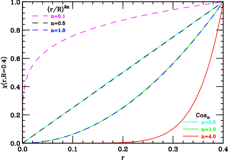
Figure 1: The different shapes of the isolation functions $\chi(r;R)$ for selected values of the power $n$ and with $R=0.4$. The functions $\chi(r;R)$ in Eqs. (3) and (4) are labelled as $(r/R)^{2n}$ (dashed lines) and Cos_n (solid lines), respectively.

The radius $R$ of the isolation cone is fixed at $R=0.4$. We study the isolation parameter dependence by considering values of $E_{T\,{\rm max}}$ in the range between 2 GeV and 10 GeV (in this section we mainly show results at the extreme values in this range). In the case of smooth cone isolation, we use the isolation function $\chi(r;R)$ in Eq. (4) and we examine the cross section dependence on the power $n$ that controls the shape of $\chi(r;R)$. In Fig. 1 we show the $r$ dependence of the isolation function for some selected values of the power $n$ and the fixed value $R=0.4$ of the radius of the isolation cone. We note that the value $R=0.4$ is sufficiently small so that the two isolation functions in Eqs. (3) and (4) quantitatively coincide at the percent level in the case with $n=1$.

We present perturbative QCD results for both standard and smooth isolation and, in particular, we perform comparisons by using the same value of the isolation parameter $E_{T\,{\rm max}}$ for both criteria. The comparison between the two criteria can also be performed differently. For instance, having fixed the values of $R$ and $E_{T\,{\rm max}}$ for standard isolation, one can use different values of isolation parameters ($R,E_{T\,{\rm max}}$ and $n$) for smooth isolation to the purpose of trying to obtain similar quantitative results for the two criteria, as a pragmatic approach to mimic the standard cone isolation that is used in experimental conditions. We think that our comparison with the same value of $E_{T\,{\rm max}}$ (and $R$) is more informative to investigate and understand differences and similarities between perturbative QCD results for the two criteria.

The QCD results on standard cone isolation depend on the parton-to-photon fragmentation function $D_{a/\gamma}(z;\mu_{frag})$ $(a=q,{\bar{q}},g)$, $z$ being the photon momentum fraction with respect to the momentum of the fragmenting parton $a$. Owing to the isolation procedure, the value of $z$ is bounded by a minimum value $z_{\rm min}$ ($1\geq z\geq z_{\rm min}$), and this leads to a quantitative suppression of the fragmentation component of the diphoton cross section. The typical value of $z_{\rm min}$ is $z_{\rm min}\sim p_{T\gamma}/(p_{T\gamma}+E_{T\,{\rm max}})$, $p_{T\gamma}$ being the transverse momentum of the photon that is involved in the fragmentation process. In our quantitative study we use relatively-large values of $p_{T\gamma}$ (i.e., typically, $p_{T\gamma}>22$ GeV) and relatively-small values of $E_{T\,{\rm max}}$. Therefore, $z_{\rm min}$ is always large ($z_{\rm min}\raisebox{-2.58334pt}{\hbox to0.0pt{$\,\sim\,$\hss}}\raisebox{1.72218pt}{$\,>\,$}0.9$ at $E_{T\,{\rm max}}=2$ GeV, and still $z_{\rm min}\raisebox{-2.58334pt}{\hbox to0.0pt{$\,\sim\,$\hss}}\raisebox{1.72218pt}{$\,>\,$}0.7$ at $E_{T\,{\rm max}}=10$ GeV), and the suppression factor  due to $\frac{\alpha_{\mathrm{S}}}{\alpha}D_{a/\gamma}$ is sizeable (roughly one order of magnitude or more, depending on $E_{T\,{\rm max}}$) [92]. We note that at such high values of $z$ the quark (or antiquark) fragmentation function $D_{q/\gamma}$ (or $D_{{\bar{q}}/\gamma}$) is much larger (roughly by more than a factor of ten) than the gluon fragmentation function $D_{g/\gamma}$ [92]. In our calculation we consistently (according to the formal perturbative expansion) include all the fragmentation functions. However, due to the dominance of $D_{q/\gamma}$ and $D_{{\bar{q}}/\gamma}$, in all our qualitative (or semi-quantitative) comments we neglect the effect of $D_{g/\gamma}$ (i.e., we can assume that only $D_{q/\gamma}$ and $D_{{\bar{q}}/\gamma}$ contribute). We also note that, because of QCD scaling violation, at high values of $z$, $D_{a/\gamma}(z;\mu_{frag})$ increases (although weakly) by increasing $\mu_{frag}$.

2.3.1 Total cross sections at LO and NLO

We begin the presentation of our quantitative results by considering the total cross section (namely, the fiducial cross section for the applied kinematical cuts on the photons). Values of total cross sections at LO and NLO for both smooth and standard isolation are reported in Table 1.

	$E_{T\,{\rm max}}=2$ GeV		$E_{T\,{\rm max}}=10$ GeV
	$\sigma^{{\rm LO}}$  (pb)	$\sigma^{{\rm NLO}}$  (pb)	$\sigma^{{\rm LO}}$  (pb)	$\sigma^{{\rm NLO}}$  (pb)
Standard	$12.15~{}^{+14.5\,{\%}}_{-14.3\,{\%}}$	$31.1~{}^{+12.8\,{\%}}_{-12.3\,{\%}}$	$19.51~{}^{+25.0\,{\%}}_{-20.8\,{\%}}$	$33.3~{}^{+12.3\,{\%}}_{-11.3\,{\%}}$
$\left[{\rm direct}\right]$	$10.56~{}^{+10.7\,{\%}}_{-12.0\,{\%}}$	$27.30~{}^{+7.8\,{\%}}_{-9.2\,{\%}}$	$10.56~{}^{+10.7\,{\%}}_{-12.0\,{\%}}$	$18.45~{}^{-10.3\,{\%}}_{+3.8\,{\%}}$
Smooth	$10.56~{}^{+10.7\,{\%}}_{-12.0\,{\%}}$	$31.92~{}^{+12.6\,{\%}}_{-12.1\,{\%}}$	$10.56~{}^{+10.7\,{\%}}_{-12.0\,{\%}}$	$33.91~{}^{+13.0\,{\%}}_{-12.6\,{\%}}$

Table 1: Results for LO and NLO total cross sections with two values of $E_{T\,{\rm max}}$ and the photon kinematical cuts described in the text (beginning of Sect. 2.3). The results are obtained by using smooth and standard isolation (the direct component of the standard isolation cross section is also reported). The NLO smooth isolation results use the isolation function $\chi(r;R)=\left(r/R\right)^{2n}$ with $n=1$. The central values of $\sigma$ are obtained with the scale choice $\mu_{R}=\mu_{F}=\mu_{frag}=M_{\gamma\gamma}$ and the scale dependence corresponds to $\{\mu_{R}=M_{\gamma\gamma}/2$, $\mu_{F}=\mu_{frag}=2M_{\gamma\gamma}\}$ (upper values) and $\{\mu_{R}=2M_{\gamma\gamma}$ , $\mu_{F}=\mu_{frag}=M_{\gamma\gamma}/2\}$ (lower values). The last digit of each cross section value has an error of one unit from the statistical uncertainty of the numerical calculation.

Using smooth cone isolation, the total cross section at LO is $\sigma^{LO}_{\rm smooth}=10.56~{}{\rm pb}~{}^{+10.7\,{\%}}_{-12.0\,{\%}}$ (scale), where the percentage variation refers to the scale dependence of the result. We note that $\sigma^{LO}_{\rm smooth}$ is independent of $E_{T\,{\rm max}}$ and of the isolation function $\chi(r;R)$. The cross section is produced only by the initial-state $q{\bar{q}}$ channel through the partonic subprocess $q{\bar{q}}\rightarrow\gamma\gamma$, and the scale dependence of $\sigma^{LO}_{\rm smooth}$ (which is entirely due to variations of $\mu_{F}$ in the quark and antiquark PDFs) is quite small. All these features are a very crude approximation of the diphoton production dynamics.

Using standard cone isolation, the LO cross section $\sigma^{LO}_{\rm standard}$ depends on $E_{T\,{\rm max}}$ and it also depends on all the three scales $\mu_{F},\mu_{R}$ and $\mu_{frag}$ ($\mu_{R}$ and $\mu_{frag}$ enter through the fragmentation component). The scale dependence of $\sigma^{LO}_{\rm standard}$ is relatively similar to that of $\sigma^{LO}_{\rm smooth}$: we find ${}^{+14.5\,{\%}}_{-14.3\,{\%}}$ (scale) and ${}^{+25.0\,{\%}}_{-20.8\,{\%}}$ (scale) with $E_{T\,{\rm max}}=2$ GeV and $E_{T\,{\rm max}}=10$ GeV, respectively. The $E_{T\,{\rm max}}$ dependence of $\sigma^{LO}_{\rm standard}$ is instead more ‘surprising’. Considering $E_{T\,{\rm max}}=2$ GeV (very tight isolation), $\sigma^{LO}_{\rm standard}$ is slightly larger, by about 15%, than $\sigma^{LO}_{\rm smooth}$ (actually the two cross sections are very similar within the corresponding scale dependence). However, $\sigma^{LO}_{\rm standard}$ increases by a factor of about 1.6 in going from $E_{T\,{\rm max}}=2$ GeV to $E_{T\,{\rm max}}=10$ GeV and, at $E_{T\,{\rm max}}=10$ GeV, $\sigma^{LO}_{\rm standard}$ is roughly a factor of 2 larger than $\sigma^{LO}_{\rm smooth}$.

Since $\sigma^{LO}_{\rm smooth}$ does not depend on the isolation parameters ($R,n,E_{T\,{\rm max}}$), there is obviously no way to approximate (or, mimic) the quantitative value of $\sigma^{LO}_{\rm standard}$ at $E_{T\,{\rm max}}=10$ GeV by using smooth cone isolation with different isolation parameters (e.g., a value of $E_{T\,{\rm max}}$ larger than 10 GeV).

The value $E_{T\,{\rm max}}=10$ GeV is not particularly large and it cannot be regarded as a very loose isolation parameter. Therefore, on physical grounds, we do not expect two actual features of the LO result: the large difference between $\sigma^{LO}_{\rm standard}$ and $\sigma^{LO}_{\rm smooth}$ at $E_{T\,{\rm max}}=10$ GeV, and the large $E_{T\,{\rm max}}$ dependence of $\sigma^{LO}_{\rm standard}$ in going from $E_{T\,{\rm max}}=2$ GeV to $E_{T\,{\rm max}}=10$ GeV. We mean that physical events are not expected to have these features, since such features cannot be regarded as a physical consequence of the hadronic activity inside the photon isolation cones and of its detailed structure (which leads to an ensuing sensitivity to the isolation criteria). These observed LO features require some explanation, which we are going to discuss.

At the LO, in the context of standard isolation, the distinction between direct and fragmentation components is unambiguous, and the direct component exactly coincides with the entire contribution to the smooth isolation result. The double-fragmentation component always gives a small contribution (few percent at $E_{T\,{\rm max}}=10$ GeV and few permill at $E_{T\,{\rm max}}=2$ GeV) to $\sigma^{LO}_{\rm standard}$. Therefore, the $E_{T\,{\rm max}}$ dependence of $\sigma^{LO}_{\rm standard}$ is due to the single-fragmentation component, whose contribution to $\sigma^{LO}_{\rm standard}$ is small (of the order of 10%) at $E_{T\,{\rm max}}=2$ GeV (because of the suppression due to the small value of $E_{T\,{\rm max}}$) and sizeable at $E_{T\,{\rm max}}=10$ GeV. At the larger value of $E_{T\,{\rm max}}$ the direct and single-fragmentation components have the same size, but this is not due to the fact that the fragmentation function is particularly large. At the LO the direct component only involves the partonic process

$$q{\bar{q}}\rightarrow\gamma\gamma\;\;,$$ (9)

whereas the (single) fragmentation component also involves the partonic process

$$qg\rightarrow\gamma q\quad\quad(q\rightarrow\gamma+X)\;\;,$$ (10)

where the notation $q\rightarrow\gamma+X$ denotes the fragmentation of the final-state quark $q$ into a photon through $D_{q/\gamma}$ (a similar notation is used in subsequent equations for partonic subprocesses). The PDF luminosity (the detailed definition of PDF luminosities is presented in Eq. (17)) ${\cal L}_{q{\bar{q}}}$ of the initial-state direct subprocess is sizeably smaller than the luminosity ${\cal L}_{qg}$ of the initial-state fragmentation subprocess (this follows from the smaller size of the antiquark PDF with respect to the gluon PDF at small values, such as $x\sim 10^{-2}$, of parton momentum fraction $x$ in the PDFs), and the suppression due to the isolated fragmentation function $D_{q/\gamma}$ is compensated by the increased size of ${\cal L}_{qg}$ with respect to ${\cal L}_{q{\bar{q}}}$ (the suppression from $D_{q/\gamma}$ is much stronger by decreasing $E_{T\,{\rm max}}$, because $z>z_{\rm min}$ and $z_{\rm min}$ increases by decreasing $E_{T\,{\rm max}}$).

According to our discussion, the presence of the fragmentation process of Eq. (10) in the LO standard cone isolation explains the quantitative dependence of $\sigma^{LO}_{\rm standard}$ on $E_{T\,{\rm max}}$ and the quantitative differences between $\sigma^{LO}_{\rm standard}$ and $\sigma^{LO}_{\rm smooth}$. At the same time, our discussion is useful to anticipate expected features of the NLO results. The NLO calculation within smooth cone isolation includes the partonic process

$$qg\rightarrow\gamma\gamma q\;\;.$$ (11)

In the kinematical configuration where the final-state quark is inside the isolation cone of one photon, the process in Eq. (11) roughly corresponds to the LO fragmentation process of Eq. (10): therefore we expect that the NLO smooth isolation result receives a large NLO correction from this kinematical configuration of this process, in such a way to reduce the observed LO ‘deficit’ with respect to standard cone isolation (in other words, $qg\rightarrow\gamma\gamma q$ is suppressed with respect to $q{\bar{q}}\rightarrow\gamma\gamma$ by an extra power of $\alpha_{\mathrm{S}}$, but this suppression is compensated by the increased luminosity of the partonic initial state). Moreover, the kinematical configuration where the final-state quark is outside the isolation cones of both photons contributes through the process of Eq. (11) to the NLO calculation of both smooth and standard isolations. This is not a very limited kinematical region (the size $R$ of the isolation cones is not large) and, due to the large value of the ${\cal L}_{qg}$ luminosity, it gives a sizeable and $E_{T\,{\rm max}}$ independent NLO contribution to both isolation prescriptions. It follows that, for both isolation criteria, we expect large NLO corrections and a much reduced $E_{T\,{\rm max}}$ dependence with respect to the LO result. As we are going to show shortly, the expectations of our discussion are confirmed by the actual NLO results.

We note that the LO results that we have presented are obtained by using LO PDFs and the NLO BFG fragmentation functions, since LO fragmentation functions are not readily available in the default setup of the DIPHOX code. This mismatch (at the strictly formal level) of perturbative order in the fragmentation functions should not strongly affect the main features of the LO standard isolation results. More generally, standard cone isolation results are certainly affected by an additional uncertainty, which is due to the poorly known fragmentation functions, that is difficult to be estimated at the quantitative level. The recent Ref. [93] presents a very brief overview on prospects for improving the determination of the photon fragmentation functions.

The value of the NLO total cross section $\sigma^{NLO}$, including its corresponding scale variation dependence, is reported in Table 1 and Fig. 2 for two different values of $E_{T\,{\rm max}}$: $E_{T\,{\rm max}}=2$ GeV (Fig. 2-left) and $E_{T\,{\rm max}}=10$ GeV (Fig. 2-right).

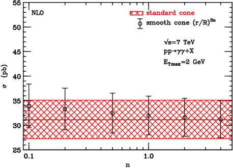
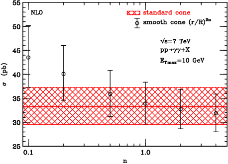
Figure 2: Value of the NLO total cross section, including scale variation dependence, for the standard (red line and band) and smooth (black error bars) isolation criteria. The photon kinematical cuts are described in the text (beginning of Sect. 2.3). The results are obtained for two different values of $E_{T\,{\rm max}}=2$ GeV (left panel) and 10 GeV (right panel). In the case of smooth cone isolation, some different values of the power $n$ ($n=0.1,0.2,0.5,1,2,4$) in the isolation function $\chi(r;R)=\left(r/R\right)^{2n}$ are considered.

In the case of smooth cone isolation, the NLO result depends on the power $n$ of the isolation function $\chi(r;R)=\left(r/R\right)^{2n}$. We postpone the discussion of the $n$ dependence and we consider the case with $n=1$. The values of the cross sections are $\sigma^{NLO}_{\rm smooth}=31.92~{}{\rm pb}~{}^{+12.6\,{\%}}_{-12.1\,{\%}}$ (scale) with $E_{T\,{\rm max}}=2$ GeV and $\sigma^{NLO}_{\rm smooth}=33.91~{}{\rm pb}~{}^{+13.0\,{\%}}_{-12.6\,{\%}}$ (scale) with $E_{T\,{\rm max}}=10$ GeV. The standard isolation cross section $\sigma^{NLO}_{\rm standard}$ is very similar to $\sigma^{NLO}_{\rm smooth}$ at both values of $E_{T\,{\rm max}}$ (see Table 1 and Fig. 2): the differences are at most at the level of 2–3% and they are sizeably smaller than the scale dependence of $\sigma^{NLO}$. The $E_{T\,{\rm max}}$ dependence is small: the NLO cross section for smooth (standard) isolation increases by a factor of 1.06 (1.07) in going from $E_{T\,{\rm max}}=2$ GeV to $E_{T\,{\rm max}}=10$ GeV. These features are in qualitative agreement with physical expectations.

The NLO radiative corrections are large (as expected from our previous discussion). Considering the ratio $K^{NLO}=\sigma^{NLO}/\sigma^{LO}$, the value of $K^{NLO}_{\rm smooth}$ is roughly 3 and the values of $K^{NLO}_{\rm standard}$ are approximately 2.6 ($E_{T\,{\rm max}}=2$ GeV) and 1.7 ($E_{T\,{\rm max}}=10$ GeV). In the case of the smooth isolation criterion, a sizeable part (roughly 50%) of the NLO total cross section is due to the $qg$ initial-state partonic channel (which is absent at the LO), and also the LO $q{\bar{q}}$ channel receives sizeable (roughly 50%) NLO corrections that increase the total cross section. In the case of standard cone isolation, at the NLO the distinction between direct and fragmentation components is no longer unambiguous (‘physical’): it depends on the factorization scheme and on the fragmentation scale $\mu_{frag}$. Within the $\overline{\rm MS}$ factorization scheme and the scale variation range that we use, the direct component contributes about 45–65% (85–90%) of $\sigma^{NLO}_{\rm standard}$ with $E_{T\,{\rm max}}=10$ GeV ($E_{T\,{\rm max}}=2$ GeV). Since $\sigma^{NLO}_{\rm standard}$ and $\sigma^{NLO}_{\rm smooth}$ are very similar, the similarity is the consequence of a non-trivial interplay between the direct and fragmentation contributions to $\sigma^{NLO}$ (especially in the case with $E_{T\,{\rm max}}=10$ GeV) and, in particular, the LO equivalence between the smooth cone result and the direct component of the standard cone result is definitely lost at the NLO.

We note that the scale dependence of the total cross section has a similar size at LO and at NLO, and it is much smaller than the size of the NLO corrections. This implies that the scale dependence of $\sigma^{NLO}$ cannot be consistently regarded as a reliable estimate of uncalculated higher-order radiative corrections to $\sigma$: the ‘true’ theoretical uncertainty of $\sigma^{NLO}$ is certainly larger than the NLO scale dependence that we have computed. A similar comment applies to the scale dependence of the results for the differential cross sections that we present in the following.

We now discuss the dependence of the smooth isolation cross section $\sigma^{NLO}_{\rm smooth}$ on the power $n$ of the isolation function $\chi(r;R)=(r/R)^{2n}$ (see Eq. (4)). The NLO results of the total cross section for some selected values of $n$ in the range $0.1\leq n\leq 4$ are reported in Fig. 2. We note that the $n$ dependence of $\sigma^{NLO}_{\rm smooth}$ is small (in particular, it is smaller than the scale dependence) within this range of values of $n$. Specifically, considering the interval $1/2<n<2$, the central value of $\sigma^{NLO}_{\rm smooth}$ varies by about 3% (10%) if $E_{T\,{\rm max}}=2$ GeV ($E_{T\,{\rm max}}=10$ GeV). Most of the qualitative features of the results in Fig.2 are consistent with physical expectations. The photons are more isolated by increasing $n$ at fixed $E_{T\,{\rm max}}$ and, consequently, $\sigma^{NLO}_{\rm smooth}$ monotonically decreases (in agreement with the physical behaviour in Eq. (8)). Moreover, by decreasing $E_{T\,{\rm max}}$ the photons are more isolated and consequently the total cross section is less sensitive to variations of the power $n$. Nonetheless, we note that, by decreasing the value of $n$, $\sigma^{NLO}_{\rm smooth}$ tends to become larger than $\sigma^{NLO}_{\rm standard}$, thus violating the physical constraint in Eq. (5). This feature deserves some comments, which are presented below.

The perturbative dependence of $\sigma_{\rm smooth}$ at very small ($n\ll 1$) or very large ($n\gg 1$) values of $n$ can be understood in relatively-simple terms. If $n$ is very small, the isolation function $\chi(r;R)=(r/R)^{2n}$ is approximately equal to unity with the exception of the angular region of very small values of $r$: therefore, the $n$ dependence of $\sigma_{\rm smooth}$ is very sensitive to radiation of partons that are collinear to the photon direction. If $n$ is very large, the isolation function very strongly suppresses parton radiation inside the photon isolation cone: therefore, the $n$ dependence of $\sigma_{\rm smooth}$ is very sensitive to soft parton radiation. The dominant effects of soft and collinear radiation can be easily computed at NLO (see Refs. [26, 57, 94]). We consider the NLO correction $\delta^{NLO}=(\sigma^{NLO}-\sigma^{LO})/\sigma^{LO}$, and we limit ourselves to sketch the dominant $n$ dependence of the soft ($\delta^{NLO,{\rm soft}}_{\rm smooth}$) and collinear ($\delta^{NLO,{\rm coll}}_{\rm smooth}$) contribution to $\delta^{NLO}$ within smooth isolation. We have

$$\delta^{NLO,{\rm soft}}_{\rm smooth} \propto -\;\alpha_{\mathrm{S}}\,R^{2}\left(\ln\left(\frac{Q}{E_{T\,{\rm max}}}\right)+n\right)\;,\quad\,(n\gg 1)\;\;,$$ (12)

$$\delta^{NLO,{\rm coll}}_{\rm smooth} \propto +\;\frac{\alpha_{\mathrm{S}}}{n}\;\frac{E_{T\,{\rm max}}}{Q}\;\;,\quad\quad\quad\quad\quad\quad\quad\quad(n\ll 1)\;\;,$$ (13)

where $Q$ is the typical hard scale of the cross section (the scale is of the order of the minimum value of $p_{T\gamma}^{hard}$) and we have considered small values of $E_{T\,{\rm max}}$ (by neglecting relative corrections of ${\cal O}(E_{T\,{\rm max}}/Q)$).

The proportionality factor that is not explicitly denoted on the right-hand side of Eq. (12) depends on the LO cross section for the partonic process $q{\bar{q}}\rightarrow\gamma\gamma$. The soft contribution in Eq. (12) is negative. It is due to a strong kinematical mismatch between (negative) soft virtual radiation (one-loop corrections in the subprocess $q{\bar{q}}\rightarrow\gamma\gamma$), which is not affected by isolation, and (positive) soft real radiation (the subprocess $q{\bar{q}}\rightarrow g\gamma\gamma$ at the tree level), which is strongly suppressed by isolation. We note that $\delta^{NLO,{\rm soft}}_{\rm smooth}$ is proportional to $n$, so that eventually $\sigma^{NLO}_{\rm smooth}$ diverges to ‘$-~{}\infty$’ in the limit $n\rightarrow+\infty$. This NLO divergence is the perturbative signal of the infrared unsafety of the isolated cross section in the limit of completely isolated photons (no accompanying transverse energy inside the isolation cone). We observe that $\delta^{NLO,{\rm soft}}_{\rm smooth}$ is proportional to $R^{2}$, so that the soft contribution is strongly suppressed if the photon isolation cone has a small radius $R$. We also note that $\delta^{NLO,{\rm soft}}_{\rm smooth}$ is due to subprocesses with a $q{\bar{q}}$ initial state. The subprocess $qg\rightarrow q\gamma\gamma$ is formally subdominant in the soft limit ($n\gg 1$), but it represents a sizeable quantitative correction to $\delta^{NLO,{\rm soft}}_{\rm smooth}$ because of the increased PDF luminosity of the $qg$ initial state. The $R^{2}$-suppressed dependence of $\delta^{NLO,{\rm soft}}_{\rm smooth}$ and the large size of the (positive) correction to it from the $qg$ initiated subprocess explain why the results for $\sigma^{NLO}_{\rm smooth}$ in Fig. 2 have a small dependence on $n$ at relatively-large values of $n$ (e.g., $n\simeq 4$).

The collinear contribution in Eq. (13) is relevant to discuss the $n$ dependence of the results in Fig. 2 at small values of $n$. We note that the NLO contributions from the initial-state $q{\bar{q}}$ channel (e.g., $q{\bar{q}}\rightarrow g\gamma\gamma$) are subdominant in the limit $n\ll 1$. The contribution in Eq. (13) is due to real radiation of a collinear quark or antiquark inside the photon isolation cone through the partonic processes $qg\rightarrow q\gamma\gamma$ and ${\bar{q}}g\rightarrow{\bar{q}}\gamma\gamma$ (the proportionality factor that is not explicitly denoted in the right-hand side of Eq. (13) depends on the LO cross section for the partonic processes $qg\rightarrow q\gamma$ and ${\bar{q}}g\rightarrow{\bar{q}}\gamma$). Therefore, $\delta^{NLO,{\rm coll}}_{\rm smooth}$ is positive and independent of $R$. Moreover, $\delta^{NLO,{\rm coll}}_{\rm smooth}$ is proportional to $E_{T\,{\rm max}}$, so that its induced $n$ dependence is reduced by decreasing $E_{T\,{\rm max}}$ (in agreement with the results in Fig. 2 at small $n$). Owing to its dependence on $n$, $\delta^{NLO,{\rm coll}}_{\rm smooth}$ sizeably increases by decreasing $n$ at fixed $E_{T\,{\rm max}}$ and, eventually, $\delta^{NLO,{\rm coll}}_{\rm smooth}$ (and, consequently, $\sigma^{NLO}_{\rm smooth}$) diverges to ‘$+\infty$’ in the limit $n\rightarrow 0$. Since $\sigma^{NLO}_{\rm smooth}$ becomes arbitrarily large by decreasing $n$, it is obvious that at sufficiently small values of $n$ the physical requirement $\sigma_{\rm smooth}<\sigma_{\rm standard}$ (see Eq. (5)) is unavoidably violated. This misbehaviour of $\sigma^{NLO}_{\rm smooth}$ at small values of $n$ implies that beyond-NLO contributions are relevant. Indeed, each higher-order contribution is equally misbehaved at $n\ll 1$: the N^kLO correction is proportional to $(\alpha_{\mathrm{S}}/n)^{k}$ (because of multiple collinear radiation inside the photon isolation cone) an it cannot be regarded as a small correction if $n\raisebox{-2.58334pt}{\hbox to0.0pt{$\,\sim\,$\hss}}\raisebox{1.72218pt}{$\,<\,$}\alpha_{\mathrm{S}}$ (i.e., $n\raisebox{-2.58334pt}{\hbox to0.0pt{$\,\sim\,$\hss}}\raisebox{1.72218pt}{$\,<\,$}0.1$). In principle, the perturbative treatment at small values of $n$ can be improved by a proper all-order resummation of these collinear contributions of ${\cal O}((\alpha_{\mathrm{S}}/n)^{k})$. However, such resummation treatment cannot be pursued for arbitrarily small values of $n$ since it unavoidably fails in the limit $n\rightarrow 0$, because of non-perturbative photon fragmentation effects (smooth isolation with $n=0$ requires photon fragmentation functions since it is equivalent to standard isolation).

We can draw some conclusions from our discussion on small values of $n$. Owing to the physical requirements in Eqs. (5) and (8), in principle cross sections for standard and smooth isolation tend to agree at very small values of $n$. However, fixed-order QCD computations for smooth isolation are not reliable if $n\ll 1$ (they are affected by large higher-order corrections) and, in particular, they can violate the physical constraint in Eq. (5). In practice, to the purpose of approximating the standard isolation criterion within fixed-order QCD calculations it is more appropriate to consider smooth isolation with values of $n$ that are not too small. From the results in Fig. 2, we can conclude that the total cross sections $\sigma^{NLO}_{\rm smooth}$ and $\sigma^{NLO}_{\rm standard}$ quantitatively agree if $n\simeq 1$.

In the following we consider differential cross sections with respect to various kinematical variables and we limit ourselves to present smooth isolation results with $n=1$. We have checked that the shape of the various NLO kinematical distributions is very little affected by variations of $n$ within the range $0.1\raisebox{-2.58334pt}{\hbox to0.0pt{$\,\sim\,$\hss}}\raisebox{1.72218pt}{$\,<\,$}n\raisebox{-2.58334pt}{\hbox to0.0pt{$\,\sim\,$\hss}}\raisebox{1.72218pt}{$\,<\,$}4$. At the NLO, variations of $n$ basically produce overall normalization effects, whose size corresponds to the $n$ dependence of $\sigma^{NLO}_{\rm smooth}$ that is observed in Fig. 2.

2.3.2 Differential cross sections at the LO

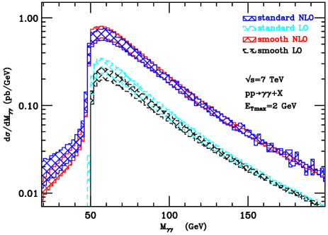
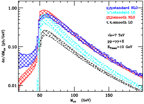
Figure 3: The $M_{\gamma\gamma}$ differential cross section for $E_{T\,{\rm max}}=2$ GeV (left panel) and $E_{T\,{\rm max}}=10$ GeV (right panel) and with the same photon kinematical cuts as in Fig. 2. The scale variation bands of the LO and NLO results for smooth and standard isolation are as follows: LO smooth isolation (black dashed), LO standard isolation (light-blue dashed), NLO smooth isolation (red solid) and NLO standard isolation (blue solid).

In Fig. 3 we present the LO and NLO results (including their scale variation dependence) for the differential cross section with respect to the diphoton invariant mass $M_{\gamma\gamma}$. We consider two different values, 2 GeV (Fig. 3-left) and 10 GeV (Fig. 3-right), of $E_{T\,{\rm max}}$ and we use both standard and smooth isolation. In Fig. 4 we present the analogous results for the differential cross section with respect to the angular variable $\cos\theta^{*}$ in the Collins–Soper rest frame. The results in Figs. 3 and 4 are obtained by numerical integration over small bins in $M_{\gamma\gamma}$ and $\cos\theta^{*}$, respectively: we use bins of constant size equal to 2 GeV for $M_{\gamma\gamma}$ and 0.08 for $\cos\theta^{*}$. In the following we discuss LO and NLO differential cross sections in turn. At the LO, we preliminarily note that standard and smooth isolation results for the differential cross sections have qualitatively similar shapes, with differences of the overall normalization that are quite similar to the quantitative differences (which we have previously discussed) of the corresponding LO total cross sections.

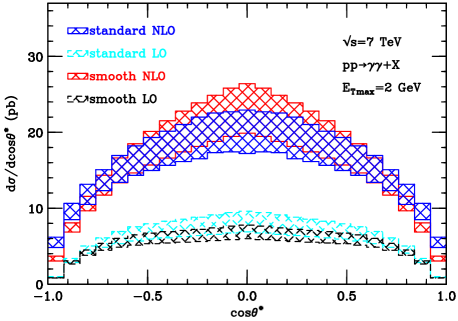
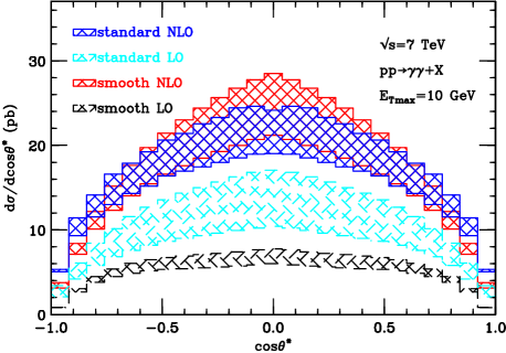
Figure 4: The $\cos\theta^{*}$ differential cross section for $E_{T\,{\rm max}}=2$ GeV (left panel) and $E_{T\,{\rm max}}=10$ GeV (right panel) and with the same photon kinematical cuts as in Fig. 2. The scale variation bands of the LO and NLO results for smooth and standard isolation are as follows: LO smooth isolation (black dashed), LO standard isolation (light-blue dashed), NLO smooth isolation (red solid) and NLO standard isolation (blue solid).

We first consider smooth cone isolation. Owing to transverse-momentum conservation in the corresponding LO partonic process $q{\bar{q}}\rightarrow\gamma\gamma$, the diphoton azimuthal separation is $\Delta\Phi_{\gamma\gamma}=\pi$ and the transverse momentum of the diphoton system is $p_{T\gamma\gamma}=0$. The corresponding differential cross sections $d\sigma^{LO}_{\rm smooth}/dx$, with $x=\Delta\Phi_{\gamma\gamma}$ or $x=p_{T\gamma\gamma}$, are simply proportional to a $\delta$-function ($\delta(\Delta\Phi_{\gamma\gamma}-\pi)$ or $\delta(p_{T\gamma\gamma})$) and the proportionality factor is the LO total cross section $\sigma^{LO}_{\rm smooth}$. The double differential cross section with respect to $M_{\gamma\gamma}$ and the scattering angle $\theta_{S}$ is

$$\frac{d\sigma^{LO}_{\rm smooth}}{dM_{\gamma\gamma}^{2}\;d|\!\cos\theta_{S}|}\propto\frac{\alpha^{2}}{s^{2}}\;g_{q{\bar{q}}}(\theta_{S})\;\sum_{q}e_{q}^{4}\;{\cal L}_{q{\bar{q}}}(\tau;\mu_{F})\;\;,$$ (14)

where $\sqrt{s}$ is the centre–of–mass energy of the hadronic collision (e.g., $\sqrt{s}=7$ TeV as in Fig. 3), $\tau=M_{\gamma\gamma}^{2}/s$ and the photon scattering angle $\theta_{S}$ is defined in the centre–of–mass frame of the LO partonic collision, and it is related to the diphoton rapidity separation $\Delta y_{\gamma\gamma}$:

$$|\!\cos\theta_{S}|=\tanh\left(\frac{|\Delta y_{\gamma\gamma}|}{2}\right)\;\;.$$ (15)

We remark that, in the case of the LO smooth isolation cross section in Eq. (14), $\theta_{S}$ and the Collins–Soper polar angle $\theta^{*}$ actually coincides ($|\!\cos\theta_{S}|=|\!\cos\theta^{*}|$), since $p_{T\gamma\gamma}=0$. In the right-hand side of Eq. (14) we have not denoted an overall proportionality factor of order unity, which is independent of the kinematical variables $s,M_{\gamma\gamma}$ and $\theta_{S}$. The angular dependent function $g_{q{\bar{q}}}(\theta_{S})$ is

$$g_{q{\bar{q}}}(\theta_{S})=\frac{2\,(1+\cos^{2}\theta_{S})}{1-\cos^{2}\theta_{S}}\;\;,$$ (16)

and it is specific for the angular distribution that is dynamically produced by the partonic process $q{\bar{q}}\rightarrow\gamma\gamma$. The function ${\cal L}_{q{\bar{q}}}(\tau;\mu_{F})$ is the $q{\bar{q}}$ PDF luminosity and $e_{q}$ is the quark electric charge in units of the positron charge ($e_{q}=2/3$ for up-type quarks). The PDF luminosity for the collision of two partons $a$ and $b$ is defined as

$${\cal L}_{ab,h_{1}h_{2}}(\tau;\mu_{F})\equiv\int_{0}^{1}\frac{dx_{1}}{x_{1}}\int_{0}^{1}\frac{dx_{2}}{x_{2}}\left[f_{a/h_{1}}(x_{1},\mu_{F})f_{b/h_{2}}(x_{2},\mu_{F})+\bigl{(}a\leftrightarrow b\bigr{)}\right]\;\delta(\tau-x_{1}x_{2})\;\;,$$ (17)

where $f_{a/h}(x,\mu_{F})$ is the PDF of the parton $a$ in the hadron $h$.

A distinctive feature of the right-hand side of Eq. (14) and, hence, of the double differential cross section is its exactly factorized dependence on $M_{\gamma\gamma}$ and $\cos\theta_{S}$. The $M_{\gamma\gamma}$ dependence is controlled by the luminosity ${\cal L}_{q{\bar{q}}}$: by decreasing $M_{\gamma\gamma}$, ${\cal L}_{q{\bar{q}}}$ rapidly increases. The $\cos\theta_{S}$ (or $\cos\theta^{*}$) dependence is controlled by $g_{q{\bar{q}}}(\theta_{S})$: by increasing $|\!\cos\theta_{S}|$, $g_{q{\bar{q}}}$ sharply increases and it becomes singular at $|\!\cos\theta_{S}|=1$ (because of the ‘unphysical’ behaviour of $2\rightarrow 2$ ‘massless’ parton scattering). The computation of the single differential cross sections $d\sigma/dM_{\gamma\gamma}$ and $d\sigma/d\cos\theta^{*}$ requires the application of kinematical cuts to select the hard-scattering regime (i.e., values of $M_{\gamma\gamma}$ in the perturbative region and values of $\cos\theta^{*}$ sufficiently far from the forward/backward scattering singularity). The simplest type of kinematical cuts is a minimum value of $M_{\gamma\gamma}$ and a maximum value of $|\!\cos\theta_{S}|$. These kinematical cuts, which preserve the factorized structure of Eq. (14) with respect to the $M_{\gamma\gamma}$ and $\cos\theta_{S}$ dependence, lead to differential cross sections $d\sigma/dM_{\gamma\gamma}$ and $d\sigma/d\cos\theta^{*}$ that are simply proportional to ${\cal L}_{q{\bar{q}}}(\tau)$ and $g_{q{\bar{q}}}(\theta^{*})$, respectively. The shapes of these differential cross sections are different (especially in the case of the $\cos\theta^{*}$ distribution) from those observed in Figs. 3 and 4. The differences originate from the kinematical cuts on the photon transverse momenta and rapidities that are described at the beginning of Sect. 2.3, and that are actually used in the computation of the differential cross sections of Figs. 3 and 4.

We first discuss the effect of the transverse-momentum ($p_{T}$) cuts $p_{T\gamma}^{hard}\geq p_{H}$ (specifically $p_{H}=25$ GeV) and $p_{T\gamma}^{soft}\geq p_{S}$ (specifically $p_{S}=22$ GeV). Since $p_{T\gamma\gamma}=0$ (i.e., $p_{T\gamma}^{hard}=p_{T\gamma}^{soft}$), only the value of $p_{H}$ is effective, and we have the LO constraint

$$M_{\gamma\gamma}\;\sin\theta_{S}\geq M^{LO}_{\rm dir}\;\;,$$ (18)

where $M^{LO}_{\rm dir}=2p_{H}$ (specifically $M^{LO}_{\rm dir}=50$ GeV) and we have simply used $2p_{T\gamma}^{hard}=M_{\gamma\gamma}\;\sin\theta_{S}$. Since $\sin\theta_{S}<1$ and $M_{\gamma\gamma}^{2}<s$, the constraint in Eq. (18) implies a lower boundary $M_{\gamma\gamma}\geq M^{LO}_{\rm dir}$ on $M_{\gamma\gamma}$ (the LO smooth isolation cross section in Fig. 3 vanishes for $M_{\gamma\gamma}<50$ GeV) and an upper boundary $|\!\cos\theta_{S}|<\sqrt{1-(M^{LO}_{\rm dir})^{2}/s}$ on $|\!\cos\theta_{S}|$ (this corresponds to $1-|\!\cos\theta_{S}|\raisebox{-2.58334pt}{\hbox to0.0pt{$\,\sim\,$\hss}}\raisebox{1.72218pt}{$\,<\,$}3\cdot 10^{-5}$ in Fig. 4). More importantly, the constraint in Eq. (18) correlates the $M_{\gamma\gamma}$ and $\cos\theta_{S}$ dependencies, thus destroying the factorized structure in the right-hand side of Eq. (14) and leading to relevant effects on the shape of the single differential cross sections.

A relevant effect regards $d\sigma/dM_{\gamma\gamma}$ in the region close to the LO threshold $M^{LO}_{\rm dir}$. At fixed values of $M_{\gamma\gamma}$, the constraint in Eq. (18) leads to an upper limit, $|\!\cos\theta_{S}|<\sqrt{1-(M^{LO}_{\rm dir}/M_{\gamma\gamma})^{2}}$, that strongly suppresses the integration region over $\cos\theta_{S}$ if $M_{\gamma\gamma}\rightarrow M^{LO}_{\rm dir}$. The increase of $d\sigma^{LO}/dM_{\gamma\gamma}$ (due to ${\cal L}_{q{\bar{q}}}$) for decreasing values of $M_{\gamma\gamma}$ is thus damped by this phase space suppression: $d\sigma^{LO}_{\rm smooth}/dM_{\gamma\gamma}$ reaches a maximum value (in the region close to $M_{\gamma\gamma}\sim M^{LO}_{\rm dir}$) and then it sharply decreases and it vanishes (proportionally to $\sqrt{M_{\gamma\gamma}^{2}-(M^{LO}_{\rm dir})^{2}}\;$) at $M_{\gamma\gamma}=M^{LO}_{\rm dir}$. This LO behaviour of $d\sigma/dM_{\gamma\gamma}$ is visible in the smooth isolation results of Fig. 3. Actually, the vanishing behaviour of $d\sigma^{LO}/dM_{\gamma\gamma}$ in the limit $M_{\gamma\gamma}\rightarrow M^{LO}_{\rm dir}$ is so steep that it is not clearly recognizable in the invariant-mass bin 50 GeV$<M_{\gamma\gamma}<52$ GeV closest to $M^{LO}_{\rm dir}=$50 GeV. This vanishing behaviour is more evident by using $M_{\gamma\gamma}$-bins with a much smaller bin size (see Fig. 10 at the end of Sect. 2.3.3).

The effect of the $p_{T}$ cut constraint in Eq. (18) on $d\sigma/d\cos\theta^{*}$ is even much more relevant than the effect on $d\sigma/dM_{\gamma\gamma}$. In the computation of $d\sigma^{LO}_{\rm smooth}/d\cos\theta_{S}$ from Eq. (14), the PDF luminosity ${\cal L}_{q{\bar{q}}}(\tau=M_{\gamma\gamma}^{2}/s)$ is integrated over $M_{\gamma\gamma}$ up to a lower limit, $M_{\gamma\gamma}>M^{LO}_{\rm dir}/\sin\theta_{S}$, that depends on $\theta_{S}$: therefore large values of $|\!\cos\theta_{S}|$ are suppressed, while small values of $|\!\cos\theta_{S}|$ are relatively enhanced by the increasing size of the PDF luminosity for decreasing values of $M_{\gamma\gamma}$. This PDF modulation of the $\cos\theta_{S}$ dependence has exactly the opposite qualitative effect with respect to the $\cos\theta_{S}$ dependence of the partonic angular distribution $g_{q{\bar{q}}}(\theta_{S})$. It turns out that the PDF modulation effect quantitatively dominates, and $d\sigma/d\cos\theta^{*}$ has a bell (concave) shape (see Fig. 4) rather than the inverse-bell (convex) shape of the angular distribution $g_{q{\bar{q}}}(\theta_{S})$ of the underlying partonic process. We note that, varying $\cos\theta_{S}$ over a wide range around the central region (say, $|\!\cos\theta_{S}|\raisebox{-2.58334pt}{\hbox to0.0pt{$\,\sim\,$\hss}}\raisebox{1.72218pt}{$\,<\,$}0.5$), the lower limit on the PDF integration varies in a restricted range ($M^{LO}_{\rm dir}<M_{\gamma\gamma}\raisebox{-2.58334pt}{\hbox to0.0pt{$\,\sim\,$\hss}}\raisebox{1.72218pt}{$\,<\,$}M^{LO}_{\rm dir}/0.8$): this implies that the results of Fig. 4 for $d\sigma/d\cos\theta^{*}$ in the region $|\!\cos\theta_{S}|\raisebox{-2.58334pt}{\hbox to0.0pt{$\,\sim\,$\hss}}\raisebox{1.72218pt}{$\,<\,$}0.5$ are quite sensitive to the behaviour of the corresponding double differential cross section in a very limited range (50 GeV$<M_{\gamma\gamma}\raisebox{-2.58334pt}{\hbox to0.0pt{$\,\sim\,$\hss}}\raisebox{1.72218pt}{$\,<\,$}60$ GeV) of $M_{\gamma\gamma}$.

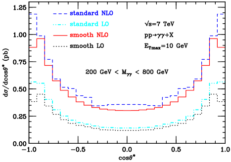
Figure 5: The $\cos\theta^{*}$ differential cross section for $E_{T\,{\rm max}}=10$ GeV and with the constraint $200~{}GeV<M_{\gamma\gamma}<800$ GeV in addition to the same photon kinematical cuts as in Fig. 4. The results, which are obtained with the scales $\mu_{R}=M_{\gamma\gamma}/2$ and $\mu_{F}=\mu_{frag}=2M_{\gamma\gamma}$, are as follows: LO smooth isolation (black dotted), LO standard isolation (light-blue dash-dotted), NLO smooth isolation (red solid) and NLO standard isolation (blue dashed).

From our discussion it follows that the PDF modulation effect on the shape of $d\sigma/d\cos\theta^{*}$ can be reduced by applying an additional kinematical cut on $M_{\gamma\gamma}$, namely, $M_{\gamma\gamma}>M_{\gamma\gamma}^{\rm min}$ with a fixed ($\theta_{S}$ independent) value $M_{\gamma\gamma}^{\rm min}$, and by selecting sufficiently large values of $M_{\gamma\gamma}^{\rm min}$. In particular, increasing $M_{\gamma\gamma}^{\rm min}$ one can eventually recover the qualitative $\theta_{S}$ dependence due to $g_{q{\bar{q}}}(\theta_{S})$. For illustrative purpose, in Fig. 5 we present the results for $d\sigma/d\cos\theta^{*}$ with the same kinematical cuts as in Fig. 4-right ($E_{T\,{\rm max}}=10$ GeV) and the additional constraint 200 GeV$<M_{\gamma\gamma}<800$ GeV (i.e., $M_{\gamma\gamma}^{\rm min}=200$ GeV). We see that the shape of $d\sigma/d\cos\theta^{*}$ in Fig. 5 is much different from that in Fig. 4-right and it is qualitatively more similar to the shape of $g_{q{\bar{q}}}(\theta_{S})$. The constraint $M_{\gamma\gamma}<800$ GeV has a negligible quantitative effect on the shape of $d\sigma/d\cos\theta^{*}$. At the LO, the additional constraint $M_{\gamma\gamma}>200$ GeV implies that the $p_{T}$ cuts have no effect on the shape of $d\sigma^{LO}_{\rm smooth}/d\cos\theta^{*}$ in the region where $|\!\cos\theta^{*}|\raisebox{-2.58334pt}{\hbox to0.0pt{$\,\sim\,$\hss}}\raisebox{1.72218pt}{$\,<\,$}0.97$: within this $\cos\theta^{*}$ region, $d\sigma^{LO}_{\rm smooth}/d\cos\theta^{*}$ follows the shape of $g_{q{\bar{q}}}(\theta_{S})$, modulo a PDF effect that is due to the kinematical cuts on the photon rapidities (the effect of the rapidity cuts is discussed below). We can also comment on the diphoton production study that is presented in Ref. [27] (see Sect. III.11 therein). That study uses the kinematical cuts $p_{T\gamma}^{hard}\geq 40$ GeV, $p_{T\gamma}^{soft}\geq 30$ GeV and 100 GeV$<M_{\gamma\gamma}<160$ GeV, which correspond to $M^{LO}_{\rm dir}=80$ GeV and $M_{\gamma\gamma}^{\rm min}=100$ GeV (note that $M_{\gamma\gamma}^{\rm min}$ is much closer to $M^{LO}_{\rm dir}$ with respect to the cuts considered in Fig. 5). The corresponding differential cross section $d\sigma/d\cos\theta^{*}$ (see Fig. III.50 in Ref. [27]) has a maximum value at $|\!\cos\theta^{*}|\sim 0.6$, and a shape that is somehow intermediate between those in Figs. 4 and 5: this behaviour is in agreement with the expectation from our discussion.

Our discussion and the results in Figs. 4 and 5 evidently show that the shape of $d\sigma/d\cos\theta^{*}$ can be strongly affected by the applied kinematical cuts as the consequence of a non-trivial interplay between underlying hard-scattering dynamics and PDF behaviour.

The results in Figs. 3 and 4 are obtained by also including the photon rapidity cut $|y_{\gamma}|<y_{M}$ (specifically $y_{M}=2.37$) in addition to the $p_{T}$ cuts (see Eq. (18)) that we have just discussed. The photon rapidity cut reduces the size of the cross sections but, since the value of $y_{M}$ is sufficiently large, the overall qualitative shape of the differential cross sections is basically unchanged. More precisely, the rapidity cut leads to the LO upper boundaries $|\!\cos\theta_{S}|<{\rm tanh}(y_{M})$ ($|\!\cos\theta_{S}|\raisebox{-2.58334pt}{\hbox to0.0pt{$\,\sim\,$\hss}}\raisebox{1.72218pt}{$\,<\,$}0.98$ in Fig. 4) and $M_{\gamma\gamma}<e^{-y_{M}}{\sqrt{s}}$ ($M_{\gamma\gamma}\raisebox{-2.58334pt}{\hbox to0.0pt{$\,\sim\,$\hss}}\raisebox{1.72218pt}{$\,<\,$}650$ GeV with $y_{M}=2.37$ and ${\sqrt{s}}=7$ TeV) on $\cos\theta_{S}$ and $M_{\gamma\gamma}$, respectively, and it modifies the form of the PDF luminosity contribution in Eq. (14). The modification amounts to the replacement ${\cal L}_{ab}(\tau)\rightarrow{\cal L}_{ab}(\tau;y_{max})$, where the customary PDF luminosity ${\cal L}_{ab}(\tau)$ is replaced by a PDF luminosity with ‘rapidity restriction’. The rapidity restricted luminosity ${\cal L}_{ab}(\tau;y_{max})$ is simply obtained by inserting the constraint $|\ln(x_{1}/x_{2})|<2y_{max}$ in the $\{x_{1},x_{2}\}$ integration region of Eq. (17) (at the LO, the rapidity $y_{\gamma\gamma}$ of the diphoton system is $2y_{\gamma\gamma}=\ln(x_{1}/x_{2})$). The value of $y_{max}$ is related to the photon rapidity cut, $y_{max}=y_{M}-|\Delta y_{\gamma\gamma}|/2$, and it depends on the diphoton rapidity separation $\Delta y_{\gamma\gamma}$ and, hence, on $\cos\theta_{S}$ (through Eq. (15)). Therefore, the rapidity restriction produces a suppression of the PDF luminosity contribution, and the suppression is larger at larger values of $|\!\cos\theta_{S}|$.

We now consider LO kinematical distributions within standard cone isolation. The LO differential cross sections $d\sigma^{LO}_{\rm standard}$ are obtained by combining the direct and fragmentation components, $d\sigma^{LO}_{\rm standard}=d\sigma^{LO}_{\rm dir}+d\sigma^{LO}_{\rm frag}$, and the direct component contribution $d\sigma^{LO}_{\rm dir}$ is exactly equal to $d\sigma^{LO}_{\rm smooth}$.

Many features of the fragmentation component contribution $d\sigma^{LO}_{\rm frag}$ are similar to those of $d\sigma^{LO}_{\rm smooth}$, and we only note the main differences. In the fragmentation component the photon is accompanied by collinear hadronic fragments and, therefore, we have $\Delta\Phi_{\gamma\gamma}=\pi$ (as in the case of smooth cone isolation at LO), while $p_{T\gamma\gamma}\neq 0$ (at variance with respect to smooth cone isolation). Moreover, due to the isolation procedure, we have $p_{T\gamma\gamma}<E_{T\,{\rm max}}$. Since $p_{T\gamma\gamma}\neq 0$, $\cos\theta_{S}$ (see Eq. (15)) is not exactly equal to the Collins–Soper variable $\cos\theta^{*}$: the relation between the two angular variables is $\cos\theta^{*}=\sqrt{M_{\gamma\gamma}^{2}/(M_{\gamma\gamma}^{2}+p_{T\gamma\gamma}^{2})}\,\cos\theta_{S}$ (which is valid for $\Delta\Phi_{\gamma\gamma}=\pi$). Since we are considering relatively-small values of $E_{T\,{\rm max}}$, we still have $p_{T\gamma\gamma}\ll M_{\gamma\gamma}$ and $\cos\theta^{*}\simeq\cos\theta_{S}$. The LO double differential cross section for the fragmentation component is

$$\frac{d\sigma^{LO}_{\rm frag}}{dM_{\gamma\gamma}^{2}\;d|\!\cos\theta_{S}|}\propto\frac{\alpha\,\alpha_{\mathrm{S}}(\mu_{R})}{s^{2}}\;g_{qg}(\theta_{S})\;\sum_{q}e_{q}^{2}\;{\cal D}_{qg}(\tau;z_{\rm min};\mu_{F},\mu_{frag})+\dots\;\;,$$ (19)

where

$$g_{qg}(\theta_{S})=\frac{5-\cos^{2}\theta_{S}}{2(1-\cos^{2}\theta_{S})}\;\;,$$ (20)

$${\cal D}_{qg}(\tau;z_{\rm min};\mu_{F},\mu_{frag})=\int_{z_{\rm min}}^{1}\frac{dz}{z}\;D_{q/\gamma}(z;\mu_{frag})\;{\cal L}_{qg}(\tau/z;\mu_{F})\;\;.$$ (21)

As in the case of Eq. (14), the right-hand side of Eq. (19) does not include an overall proportionality factor of order unity and we have explicitly written only the single-fragmentation contribution due to the initial-state $qg$ partonic channel (the dots in the right-hand side of Eq. (19) stand for all the other single-fragmentation and double-fragmentation contributions). As previously remarked in the context of our discussion of the total cross section $\sigma^{LO}_{\rm standard}$, when the fragmentation component is large (i.e., with a similar size as the direct component) the single-fragmentation contribution from the $qg$ initial state gives the bulk of the entire fragmentation component. The angular distribution $g_{qg}(\theta_{S})$ in Eq. (20) is due to $qg\rightarrow q\gamma$ scattering and its $\cos\theta_{S}$ dependence is similar to that of $g_{q{\bar{q}}}(\theta_{S})$ in Eq. (16).

The function ${\cal D}_{qg}$ in Eq. (21) is an ‘effective’ (with isolation) partonic luminosity, which is obtained by convoluting the $qg$ PDF luminosity ${\cal L}_{qg}$ with the quark-to-photon fragmentation function $D_{q/\gamma}$. The boundary value $z_{\rm min}$ in the convolution is due to photon isolation (in the case of the single fragmentation component, $z_{\rm min}$ is due to the isolation requirement $z>p_{T\gamma}^{soft}/(p_{T\gamma}^{soft}+E_{T\,{\rm max}})\,$) and it increases as $E_{T\,{\rm max}}$ decreases, thus leading to an increasing suppression effect of the fragmentation component as $E_{T\,{\rm max}}$ decreases (see Figs. 3 and 4).

Despite the isolation suppression, we have already remarked that the effective partonic luminosity $\frac{\alpha_{\mathrm{S}}}{\alpha}{\cal D}_{qg}(\tau;z_{\rm min})$ can still be quantitatively similar to ${\cal L}_{q{\bar{q}}}$ (and, hence, $d\sigma^{LO}_{\rm frag}$ and $d\sigma^{LO}_{\rm dir}=d\sigma^{LO}_{\rm smooth}$ can have similar size) because ${\cal L}_{qg}$ is larger than ${\cal L}_{q{\bar{q}}}$. Increasing the value of $M_{\gamma\gamma}$, the photon transverse momenta and, consequently, $z_{\rm min}$ tend to increase (unless $|\Delta y_{\gamma\gamma}|$ and, correspondingly, $|\!\cos\theta_{S}|$ have large values), therefore reducing the size of the fragmentation component. The effect is visible in the LO results of Fig. 3, which show that the relative difference between $d\sigma^{LO}_{\rm smooth}$ and $d\sigma^{LO}_{\rm standard}$ is reduced at high values of $M_{\gamma\gamma}$. The effect is also visible in the comparison between the LO results of Figs. 4-right and 5: the invariant-mass cut $M_{\gamma\gamma}>200$ GeV strongly reduces the relative contribution of the fragmentation component, unless $|\!\cos\theta^{*}|$ is large. We note that, increasing the value of $M_{\gamma\gamma}$, the relative effect of the fragmentation component also decreases because ${\cal L}_{qg}$ and ${\cal L}_{q{\bar{q}}}$ become quantitatively more similar for increasing values, $x\sim{\sqrt{\tau}}=M_{\gamma\gamma}/{\sqrt{s}}$, of the parton momentum fraction $x$.

Since $p_{T\gamma\gamma}=p_{T\gamma}^{hard}-p_{T\gamma}^{soft}\neq 0$ (in particular, $p_{T\gamma}^{hard}-p_{T\gamma}^{soft}<E_{T\,{\rm max}}$), both values, $p_{H}$ and $p_{S}$, of the $p_{T}$ cuts are effective in the case of the fragmentation component. In particular, they still lead to an LO kinematical boundary, $M_{\gamma\gamma}~{}>~{}M^{LO}_{\rm frag}$, on $M_{\gamma\gamma}$ but we have $M^{LO}_{\rm frag}<M^{LO}_{\rm dir}$. The boundary value is $M^{LO}_{\rm frag}=2\sqrt{p_{H}(p_{H}-E_{T\,{\rm max}})}\;$ if $p_{H}-E_{T\,{\rm max}}>p_{S}$, and $M^{LO}_{\rm frag}=2\sqrt{p_{H}p_{S}}\;$ if $p_{S}>p_{H}-E_{T\,{\rm max}}$. The vanishing of the LO standard isolation cross section at $M_{\gamma\gamma}~{}<~{}M^{LO}_{\rm frag}$ is visible in Fig. 3-left ($M^{LO}_{\rm frag}\simeq 48$ GeV) and Fig. 3-right ($M^{LO}_{\rm frag}\simeq 47$ GeV). The presence of two different LO thresholds, $M^{LO}_{\rm frag}$ and $M^{LO}_{\rm dir}$, for standard and smooth isolation is more evident in Fig. 6 ($M^{LO}_{\rm frag}\simeq 53$ GeV and $M^{LO}_{\rm dir}=64$ GeV), which presents the results for $d\sigma/dM_{\gamma\gamma}$ with the same kinematical cuts as in Fig. 3 but with an increased value of $p_{H}$ ($p_{T\gamma}^{hard}>p_{H}=32$ GeV).

The shape of $d\sigma^{LO}_{\rm frag}/dM_{\gamma\gamma}$ near the LO threshold is qualitatively similar to that of $d\sigma^{LO}_{\rm smooth}/dM_{\gamma\gamma}$: the maximum value and the sharp decrease of $d\sigma^{LO}_{\rm frag}/dM_{\gamma\gamma}$ for $M_{\gamma\gamma}\sim M^{LO}_{\rm frag}$ are produced by the $p_{T}$ cuts through the same kinematical mechanism that we have described in the case of the smooth isolation result. In the case of the single-fragmentation component, using $2p_{T\gamma}^{soft}=2zp_{T\gamma}^{hard}={\sqrt{z}}M_{\gamma\gamma}\sin\theta_{S}$, we can express $z_{\rm min}$ as a function of $E_{T\,{\rm max}}/(M_{\gamma\gamma}\sin\theta_{S})$ and the $p_{T}$ cuts lead to the constraints $M_{\gamma\gamma}\sin\theta_{S}>2p_{H}{\sqrt{z}}$ and ${\sqrt{z}}M_{\gamma\gamma}\sin\theta_{S}>2p_{S}$. Note that the integration region over the photon momentum fraction $z$ is limited also by the effect of the $p_{T}$ cuts. In the vicinity of the LO invariant-mass threshold, $M_{\gamma\gamma}\sim M^{LO}_{\rm frag}$, the phase space integration region over $z$ is strongly suppressed by these cuts, and the $M_{\gamma\gamma}$ distribution vanishes proportionally to $(M_{\gamma\gamma}-M^{LO}_{\rm frag})^{3/2}$. In particular, this vanishing behaviour is stronger and smoother (by a factor of $M_{\gamma\gamma}-M^{LO}_{\rm frag}$) than the LO vanishing behaviour of $d\sigma/dM_{\gamma\gamma}$ for smooth cone isolation.

The effect of the rapidity cut $|y_{\gamma}|<y_{M}$ is analogous to the case of smooth isolation: it leads to the replacement ${\cal L}_{qg}(\tau)\rightarrow{\cal L}_{qg}(\tau;y_{max})$ ($y_{max}=y_{M}-|\Delta y_{\gamma\gamma}|/2$) in the right-hand side of Eq. (21).

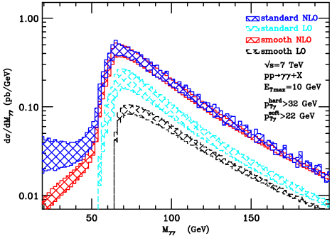
Figure 6: The $M_{\gamma\gamma}$ differential cross section for $E_{T\,{\rm max}}=10$ GeV with the same photon kinematical cuts as in Fig. 3-right and an increased cut on the minimum value of $p_{T\gamma}^{hard}$ ($p_{T\gamma}^{hard}>32$ GeV). The scale variation bands of the LO and NLO results for smooth and standard isolation are as follows: LO smooth isolation (black dashed), LO standard isolation (light-blue dashed), NLO smooth isolation (red solid) and NLO standard isolation (blue solid).

2.3.3 Differential cross sections at the NLO

We now move to discuss the NLO results for the differential cross sections. In addition to the $M_{\gamma\gamma}$ and $\cos\theta^{*}$ distributions, we present the NLO results for the differential cross sections with respect to the diphoton azimuthal separation $\Delta\Phi_{\gamma\gamma}$ (Fig. 7) and to the transverse momentum $p_{T\gamma\gamma}$ of the photon pair (Fig. 8). The NLO results in Figs. 7 and 8 are obtained by using the reference kinematical cuts described at the beginning of Sect. 2.3 (as in the case of Figs. 3 and 4). As we have previously noticed, the LO calculation leads to non-vanishing differential cross section only in specific LO kinematical subregions. Therefore, outside these LO kinematical subregions (i.e., if $M_{\gamma\gamma}<M^{LO}$, $\Delta\Phi_{\gamma\gamma}\neq\pi$ or $p_{T\gamma\gamma}>E_{T\,{\rm max}}$), the NLO results presented in Figs. 3, 6, 7 and 8 actually represent ‘effective’ LO predictions for the corresponding differential cross sections. We also note that, dealing with ‘effective’ LO predictions, the distinction between direct and fragmentation components is unambiguous in the context of standard cone isolation.

We first discuss the results for the invariant-mass distribution (Fig. 3). It is convenient to consider three different regions: the region of intermediate values of $M_{\gamma\gamma}$ (say, 45 GeV$<M_{\gamma\gamma}<65$ GeV) around the LO kinematical threshold at $M_{\gamma\gamma}\sim M^{LO}$, and the regions of higher and lower values of $M_{\gamma\gamma}$. For the purposes of the subsequent discussions, we also define

$$M^{LO}\equiv 2\sqrt{p_{H}p_{S}}\;\;.$$ (22)

Note that $M^{LO}$ is equal to (or smaller than) the minimum between the thresholds $M^{LO}_{\rm frag}$ and $M^{LO}_{\rm dir}$.

In the high-mass region where $M_{\gamma\gamma}>65$ GeV (Fig. 3), the NLO results for smooth and standard isolation are quantitatively very similar, with a scale dependence that is comparable to that of the corresponding NLO total cross sections. The NLO corrections are large for both isolation criteria and for both values of $E_{T\,{\rm max}}=2$ GeV and 10 GeV considered in Fig. 3. All these features are similar (both qualitatively and quantitatively) to those of the NLO and LO total cross sections and they have exactly the same origin, which we have already remarked in our discussion on the total cross sections. We do not repeat such a discussion on the role of the $qg$ initial-state channel and of the corresponding PDF luminosity at different perturbative orders and within the two different isolation criteria.

The NLO total cross section receives a negligible contribution from $d\sigma^{NLO}/dM_{\gamma\gamma}$ in the low-mass region ($M_{\gamma\gamma}<45$ GeV): the contribution is smaller than the scale dependence of the total cross section. The LO kinematical boundary on $M_{\gamma\gamma}$ is unphysical: it is due to the $p_{T}$ cuts on the photons but it is an artifact of the LO kinematics, which implies $\Delta\Phi_{\gamma\gamma}=\pi$. Physical diphoton events (and also corresponding partonic contributions beyond the LO) can have $\Delta\Phi_{\gamma\gamma}<\pi$: they produce non-vanishing values of $d\sigma/dM_{\gamma\gamma}$ at $M_{\gamma\gamma}<M^{LO}$, although this kinematical region is strongly suppressed by the photon $p_{T}$ cuts. Owing to energy conservation and the presence of the $p_{T}$ cuts, the low-mass region selects diphoton events with small values of $\Delta\Phi_{\gamma\gamma}$. Owing to transverse-momentum conservation, in the low-mass region these $p_{T}$ cuts effectively act also as a lower limit on $p_{T\gamma\gamma}$ or, equivalently, on the total transverse momentum of the hadronic (partonic) final-state system. Roughly speaking, low values of $M_{\gamma\gamma}$ imply small values of $\Delta\Phi_{\gamma\gamma}$ and, in turn, relatively-large values of $p_{T\gamma\gamma}$.

In general, kinematics leads to the minimal constraint

$$M_{\gamma\gamma}>M^{LO}\sin\left(\frac{\Delta\Phi_{\gamma\gamma}}{2}\right)\;\;,$$ (23)

which implies that decreasing values of $M_{\gamma\gamma}$ necessarily require decreasing values of $\Delta\Phi_{\gamma\gamma}$. The constraint in Eq. (23) is obtained by setting $\Delta y_{\gamma\gamma}=0$; larger values of $|\Delta y_{\gamma\gamma}|$ further reduce the value of $\Delta\Phi_{\gamma\gamma}$ at fixed value of $M_{\gamma\gamma}$. Eventually the kinematical lower limit on $M_{\gamma\gamma}$ is obtained by the combined effect of the $p_{T}$ cuts and the cut on the minimum angular separation, $R_{\gamma\gamma}>R_{\gamma\gamma}^{\rm min}=0.4$, between the photons. Since the value of $R_{\gamma\gamma}^{\rm min}$ is small, the lower limit on $M_{\gamma\gamma}$ is $M_{\gamma\gamma}\raisebox{-2.58334pt}{\hbox to0.0pt{$\,\sim\,$\hss}}\raisebox{1.72218pt}{$\,>\,$}M^{LO}R_{\gamma\gamma}^{\rm min}/2\simeq 10$ GeV.

As a consequence of the kinematical constraint in Eq. (23), if $M_{\gamma\gamma}\raisebox{-2.58334pt}{\hbox to0.0pt{$\,\sim\,$\hss}}\raisebox{1.72218pt}{$\,<\,$}41$ GeV ($M_{\gamma\gamma}\raisebox{-2.58334pt}{\hbox to0.0pt{$\,\sim\,$\hss}}\raisebox{1.72218pt}{$\,<\,$}33$ GeV) we have $\Delta\Phi_{\gamma\gamma}\raisebox{-2.58334pt}{\hbox to0.0pt{$\,\sim\,$\hss}}\raisebox{1.72218pt}{$\,<\,$}2.1\simeq 2\pi/3$ ($\Delta\Phi_{\gamma\gamma}\raisebox{-2.58334pt}{\hbox to0.0pt{$\,\sim\,$\hss}}\raisebox{1.72218pt}{$\,<\,$}1.6\simeq\pi/2$): therefore, due to transverse-momentum conservation, the total transverse momentum of the partonic (hadronic) final state is necessarily larger than $p_{T\gamma}^{soft}$ ($p_{T\gamma}^{hard}$). At smaller values of $M_{\gamma\gamma}$ we have $\Delta\Phi_{\gamma\gamma}\raisebox{-2.58334pt}{\hbox to0.0pt{$\,\sim\,$\hss}}\raisebox{1.72218pt}{$\,<\,$}1.4$ if $M_{\gamma\gamma}\simeq 30$ GeV and $\Delta\Phi_{\gamma\gamma}\raisebox{-2.58334pt}{\hbox to0.0pt{$\,\sim\,$\hss}}\raisebox{1.72218pt}{$\,<\,$}0.9$ if $M_{\gamma\gamma}\simeq 20$ GeV: therefore, we are dealing with a relatively collimated diphoton system that recoils against a high-$p_{T}$ hadronic (partonic) jet in the transverse-momentum plane.

Using kinematical considerations, the region of small values of $\Delta\Phi_{\gamma\gamma}$ can also be more directly related to $p_{T\gamma\gamma}$. As a consequence of transverse-momentum conservation and of the photon $p_{T}$ cuts, provided $\Delta\Phi_{\gamma\gamma}<\pi/2$ we have

$$p_{T\gamma\gamma}>\sqrt{p_{H}^{2}+p_{S}^{2}+2p_{H}p_{S}\,\cos\,(\Delta\Phi_{\gamma\gamma})}\;\;\;,\quad\quad\quad(\Delta\Phi_{\gamma\gamma}<\pi/2)\;\;.$$ (24)

This relation shows that small values of $\Delta\Phi_{\gamma\gamma}$ necessarily imply relatively-large values of $p_{T\gamma\gamma}$. For instance, if $\Delta\Phi_{\gamma\gamma}=\pi/2$ we have $p_{T\gamma\gamma}>\sqrt{p_{H}^{2}+p_{S}^{2}}$ (i.e., $p_{T\gamma\gamma}>34$ GeV if $p_{H}=25$ GeV and $p_{S}=22$ GeV), whereas at very small values of $\Delta\Phi_{\gamma\gamma}$ we have

$$p_{T\gamma\gamma}>p_{H}+p_{S}\;\;,\quad\quad\quad(\Delta\Phi_{\gamma\gamma}\simeq 0)\;\;.$$ (25)

Therefore, if $p_{H}=25$ GeV and $p_{S}=22$ GeV, the region where $\Delta\Phi_{\gamma\gamma}\simeq 0$ does not contribute to the $p_{T\gamma\gamma}$ spectrum unless $p_{T\gamma\gamma}\raisebox{-2.58334pt}{\hbox to0.0pt{$\,\sim\,$\hss}}\raisebox{1.72218pt}{$\,>\,$}47$ GeV.

In the low-mass region (Fig. 3), the scale dependence of the NLO differential cross section is larger than the corresponding dependence of the NLO total cross section, as expected from an effective LO prediction. In the case of smooth isolation, the scale dependence slightly increases by decreasing $M_{\gamma\gamma}$; at $M_{\gamma\gamma}\sim 20$ GeV the scale dependence is roughly a factor of 2 larger than the scale dependence of the NLO total cross section. The scale dependence of the standard isolation result is larger, and it increases by either decreasing $M_{\gamma\gamma}$ or increasing $E_{T\,{\rm max}}$; at $M_{\gamma\gamma}\sim 20$ GeV and $E_{T\,{\rm max}}=10$ GeV the scale dependence of the NLO differential cross section is roughly a factor of 3.6 larger than the scale dependence of the NLO total cross section. At the lower value of $E_{T\,{\rm max}}$ (2 GeV), smooth and standard isolations give similar NLO differential cross sections, within the corresponding scale variation uncertainties. At the higher value of $E_{T\,{\rm max}}$ (10 GeV), the smooth isolation result is systematically smaller than the standard isolation result and the relative difference increases by decreasing $M_{\gamma\gamma}$: the NLO results for standard isolation is roughly a factor of 3.8 (2.5) larger than the corresponding result for smooth isolation at $M_{\gamma\gamma}\sim 20$ GeV ($M_{\gamma\gamma}\sim 30$ GeV).

The observed NLO differences between smooth and standard isolation in the low-mass region (analogously to the corresponding LO differences in the high-mass region and to the LO differences of the total cross section) deserve specific comments. The NLO calculation for smooth isolation has two photons and one parton in the final state. Owing to transverse-momentum conservation, the parton can be inside the photon isolation cones only if $\Delta\Phi_{\gamma\gamma}>\pi-R\simeq 2.7$, which corresponds to $M_{\gamma\gamma}\raisebox{-2.58334pt}{\hbox to0.0pt{$\,\sim\,$\hss}}\raisebox{1.72218pt}{$\,>\,$}46$ GeV in view of the constraint in Eq. (23). Therefore, in the entire low-mass region the NLO result for smooth isolation is exactly independent of $E_{T\,{\rm max}}$, and that represents a much simplified approximation of the expected physical behaviour. The independence of $E_{T\,{\rm max}}$ also implies that the smooth isolation result is exactly equal to the result of the direct component for standard isolation. Therefore, the observed differences between the two isolation criteria are entirely due to the fragmentation component of the standard isolation calculation. The NLO result for smooth isolation (or, equivalently, for the direct component) is due to the partonic processes $q{\bar{q}}\rightarrow g\gamma\gamma$ and $qg\rightarrow q\gamma\gamma$ (or ${\bar{q}}g\rightarrow{\bar{q}}\gamma\gamma$), where the collimated diphoton system recoils against the final-state parton, and the initial-state $qg$ process gives the dominant contribution because of the larger ${\cal L}_{qg}$ PDF luminosity. The large NLO effect of the fragmentation component (especially at the higher value of $E_{T\,{\rm max}}$, which leads to a smaller suppression effect from isolation) is due to its numerous partonic processes, which, moreover, also include the $gg$ and $qq$ initial states: the corresponding partonic cross sections (although they are suppressed by isolation) can be enhanced by the size of the PDF luminosity (${\cal L}_{gg}$ and ${\cal L}_{qg}$ have a comparable size). In particular, two of these partonic processes are

$$qg\rightarrow gq\gamma\quad\quad(q\rightarrow\gamma+X)\;\;$$ (26)

and

$$gg\rightarrow{\bar{q}}q\gamma\quad\quad(q\rightarrow\gamma+X,\;\;{\rm or}\;\;{\bar{q}}\rightarrow\gamma+X)\;\;,$$ (27)

where the final-state quark (or the antiquark in the case of the $gg$ channel of Eq. (27)) is collimated with the $\gamma$ and fragments into a second photon. At low values of $M_{\gamma\gamma}$ these two partonic processes are enhanced by the relative factor $(M^{LO}/M_{\gamma\gamma})^{2}$ (its value is about 2.4 and 5.5 at $M_{\gamma\gamma}\sim 30$ GeV and $M_{\gamma\gamma}\sim 20$ GeV, respectively), which originates from the final-state perturbative singularity in the $q\gamma$ collinear limit (or ${\bar{q}}\gamma$ collinear limit in the case of the $gg$ channel of Eq. (27)). Analogous processes, namely,

$$qg\rightarrow gq\gamma\gamma$$ (28)

and

$$gg\rightarrow{\bar{q}}q\gamma\gamma\;\;,$$ (29)

where a final-state quark (or antiquark) is inside the isolation cone of one photon, contribute (and their contribution depends on $E_{T\,{\rm max}}$) to the NNLO calculation for smooth isolation. We thus expect that these processes lead to large radiative corrections (this expectation is confirmed by the NNLO results presented and discussed in Sect. 3.2; see, in particular, Fig. 11-left) and that the corresponding NNLO result removes the large differences with respect to the standard isolation result.

In summary, according to our discussion, the sizeable NLO differences between standard and smooth isolation results that are observed in the low-mass region (Fig. 3) are more an artifact of the NLO calculation than a physical effect due to the two different isolation criteria. Certainly, the achievement of high-precision QCD predictions in the low-mass region is challenging, basically because of the relatively-low value of the characteristic hard-scattering scale $M_{\gamma\gamma}$.

The region of intermediate values of $M_{\gamma\gamma}$ (45 GeV $<M_{\gamma\gamma}<65$ GeV in Fig. 3) is the region where the shape of $d\sigma/dM_{\gamma\gamma}$ is directly most sensitive to the $p_{T}$ cuts. The NLO results for smooth and standard isolation are quite similar in this region. Independently of the isolation criterion, the differential cross section starts to rapidly increase at $M_{\gamma\gamma}\simeq M^{LO}\simeq 47$ GeV and the position of the peak (the maximum of $d\sigma/dM_{\gamma\gamma}$) is basically unchanged with respect to that of the LO result for standard isolation. It is noticeable that $d\sigma/dM_{\gamma\gamma}$ starts to increase at $M_{\gamma\gamma}\simeq M^{LO}$ ($M^{LO}\simeq M^{LO}_{\rm frag}$) despite the presence of two different LO threshold, $M^{LO}_{\rm frag}$ and $M^{LO}_{\rm dir}$, that are displaced (the LO threshold at $M^{LO}_{\rm dir}$ is somehow more ‘unphysical’: it is insensitive to the value of $p_{S}$ since absolutely no partonic transverse momentum is allowed in the final state of the corresponding LO calculation). The NLO corrections are obviously large for $M_{\gamma\gamma}<M^{LO}_{\rm dir}=50$ GeV, and they are sizeable also at $M_{\gamma\gamma}>50$ GeV (for the same reason as for the high-mass region). In the case with $E_{T\,{\rm max}}=10$ GeV we note that the NLO result for smooth isolation tends to be larger than the corresponding result for standard isolation, in disagreement with the physical constraint in Eq. (5). We do not regard this behaviour as particularly worrisome since the values of $d\sigma/dM_{\gamma\gamma}$ for the two isolation criteria are basically consistent with each other within the computed scale variation uncertainties. Moreover, these scale variation effects are expected to underestimate higher-order perturbative uncertainties. Indeed, perturbative calculations in regions around unphysical fixed-order thresholds are known [60] to be generally affected by perturbative instabilities at higher orders (further comments on this point are postponed to the end of this section). In our specific case, $d\sigma/dM_{\gamma\gamma}$ is very steep in the region around the LO kinematical threshold and even the effect of little instabilities is amplified by the large slope of $d\sigma/dM_{\gamma\gamma}$. The ensuing effect on the comparison between smooth and standard isolation results can be relevant since the slopes of the two results are both large and they are different. We also add that the standard isolation results do not include the uncertainty (which is difficult to be quantified) that is due to the limited knowledge of the photon fragmentation functions (an increased value of the fragmentation functions can reduce the differences between smooth and standard isolation results in this $M_{\gamma\gamma}$ region).

We briefly comment on the results in Fig. 6, which are analogous to those in Fig. 3-right apart from having more asymmetric $p_{T}$ cuts. The value of $p_{H}$ increases in going from Fig. 3-right to Fig. 6, so that the size of the unbalance between the minimum values of the photon transverse momenta increases from $p_{H}-p_{S}=3$ GeV to $p_{H}-p_{S}=10$ GeV. The main features of the results in Figs. 3-right and 6 are very similar. In particular, we can comment on the behaviour of $d\sigma/dM_{\gamma\gamma}$ in the region of intermediate values of $M_{\gamma\gamma}$, just above $M_{\gamma\gamma}=M^{LO}$ ($M^{LO}\simeq 47$ GeV and $M^{LO}\simeq 53$ GeV in Figs. 3 and 6, respectively). The NLO results for smooth and standard isolation are very similar in this region despite the fact that the difference between the LO thresholds $M^{LO}_{\rm frag}$ ($M^{LO}_{\rm frag}=M^{LO}$) and $M^{LO}_{\rm dir}$ is larger in the case of more asymmetric cuts ($M^{LO}_{\rm dir}-M^{LO}\simeq 11$ GeV in Fig. 6, while $M^{LO}_{\rm dir}-M^{LO}\simeq 3$ GeV in Fig. 3). This similarity between the NLO results also confirms our observation in the previous paragraph that the ‘threshold’ at $M_{\gamma\gamma}\sim M^{LO}$ is somehow more ‘physical’. Even in the case of more asymmetric cuts, the NLO corrections are able to remove the relative ‘deficit’ of the LO results for smooth isolation in the vicinity of the LO threshold. Comparing Figs. 3-right and 6 we see that the slope of $d\sigma/dM_{\gamma\gamma}$ is smaller in the case of more asymmetric cuts, and the NLO results for smooth and standard isolation are more similar (in particular, the smooth isolation result does not tend to be larger than the standard isolation result, consistently with our previous comment on the behaviour observed in Fig. 3). Additional comments on symmetric and asymmetric $p_{T}$ cuts are presented in Sect. 3.

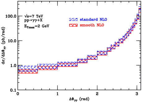
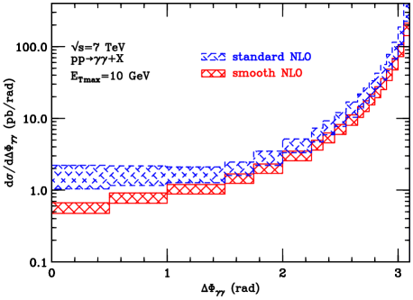
Figure 7: The NLO results (scale variation bands) for the $\Delta\Phi_{\gamma\gamma}$ differential cross section that are obtained by using the smooth (red solid band) and standard (blue dashed band) cone isolation criteria with $E_{T\,{\rm max}}=2$ GeV (left panel) and $E_{T\,{\rm max}}=10$ GeV (right panel). The photon kinematical cuts are the same as in Fig. 3.

In Fig. 7 we present the NLO results for the differential cross section with respect to the azimuthal angle separation $\Delta\Phi_{\gamma\gamma}$ of the two photons. At the LO, $\Delta\Phi_{\gamma\gamma}=\pi$ for both isolation criteria. As is well known [28], at higher perturbative orders the computation of the differential cross section is affected by large logarithmic corrections in the region near $\Delta\Phi_{\gamma\gamma}=\pi$. In this region, any fixed-order QCD result is physically not reliable, and reliable quantitative predictions for the detailed shape of the $\Delta\Phi_{\gamma\gamma}$ distribution can be recovered only through all-order perturbative resummation [42, 43] of these large logarithmic contributions. Owing to this reason, in the results of Fig. 7 we have excluded the region around $\Delta\Phi_{\gamma\gamma}=\pi$. This also implies that the NLO results in Fig. 7 (with $\Delta\Phi_{\gamma\gamma}<\pi$) actually represent ‘effective’ LO predictions for the $\Delta\Phi_{\gamma\gamma}$ distribution.

Independently of the value of $E_{T\,{\rm max}}$, we note that the $\Delta\Phi_{\gamma\gamma}$ distribution is sharply peaked at large values of $\Delta\Phi_{\gamma\gamma}$: the cross section decreases by more than one order of magnitude by decreasing $\Delta\Phi_{\gamma\gamma}$ from $\Delta\Phi_{\gamma\gamma}\sim 3$ to $\Delta\Phi_{\gamma\gamma}\sim 2.5$, and it still decreases by about one order of magnitude in going from $\Delta\Phi_{\gamma\gamma}\sim 2.5$ to $\Delta\Phi_{\gamma\gamma}\sim 0.5$. Standard and smooth isolation results have a similar scale dependence that increases from roughly $\pm 20$% at $\Delta\Phi_{\gamma\gamma}\sim 2.5$ to roughly $\pm 30$% at $\Delta\Phi_{\gamma\gamma}\sim 0.5$ (in the case of standard isolation the scale dependence also slightly increases by increasing the value of $E_{T\,{\rm max}}$). As expected from an effective LO prediction, this scale dependence is larger (by about a factor of 2–3) than the scale dependence of the NLO total cross section (the bulk of the NLO total cross section is due to the region near $\Delta\Phi_{\gamma\gamma}\sim\pi$, where the scale dependence of the $\Delta\Phi_{\gamma\gamma}$ differential cross section is reduced).

The main quantitative differences between standard and smooth isolation results appear by examining the dependence on $E_{T\,{\rm max}}$ of the $\Delta\Phi_{\gamma\gamma}$ distribution. At very small values of $E_{T\,{\rm max}}$ ($E_{T\,{\rm max}}=2$ GeV) the two isolation criteria lead to very similar results, within the corresponding scale variation uncertainties. At larger values of $E_{T\,{\rm max}}$ ($E_{T\,{\rm max}}=10$ GeV), smooth cone results tend to be smaller than standard cone results, and the differences increase by decreasing the value of $\Delta\Phi_{\gamma\gamma}$. At very small values of $\Delta\Phi_{\gamma\gamma}$, the differences are sizeable; for instance, standard NLO results are roughly a factor of 2.1 larger than smooth NLO results at $\Delta\Phi_{\gamma\gamma}\sim 0.5$. In the case of smooth isolation, the $qg$ initial-state partonic channel contributes more than the $q{\bar{q}}$ channel (because of the larger ${\cal L}_{qg}$ PDF luminosity). At high values of $\Delta\Phi_{\gamma\gamma}$ the smooth isolation result depends very weakly on $E_{T\,{\rm max}}$ and it is very similar (though it is not exactly equal) to the direct component of the standard isolation result. As previously mentioned, if $\Delta\Phi_{\gamma\gamma}<\pi-R\simeq 2.7$ the smooth isolation result is exactly independent of $E_{T\,{\rm max}}$ and it coincides with the direct component of the standard isolation cross section. Therefore, at low values of $\Delta\Phi_{\gamma\gamma}$ the NLO differences between the two isolation criteria are entirely due to the fragmentation component of the standard isolation calculation.

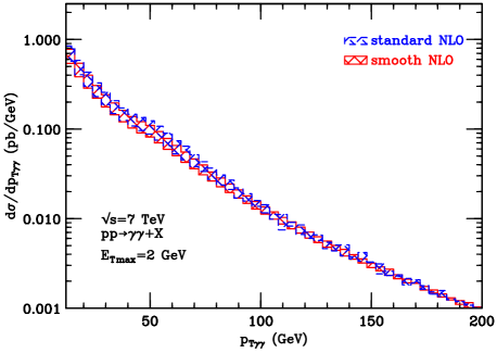
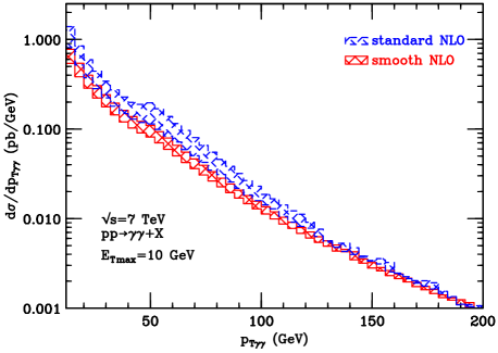
Figure 8: The NLO results (scale variation bands) for the $p_{T\gamma\gamma}$ differential cross section that are obtained by using the smooth (red solid band) and standard (blue dashed band) cone isolation criteria with $E_{T\,{\rm max}}=2$ GeV (left panel) and $E_{T\,{\rm max}}=10$ GeV (right panel). The photon kinematical cuts are the same as in Fig. 3.

In Fig. 8 we present the NLO results for the differential cross section with respect to the transverse momentum $p_{T\gamma\gamma}$ of the photon pair. At LO, as already mentioned, $p_{T\gamma\gamma}=0$ for smooth isolation while $p_{T\gamma\gamma}<E_{T\,{\rm max}}$ for standard isolation. Analogously to the case of $d\sigma/d\Delta\Phi_{\gamma\gamma}$ at $\Delta\Phi_{\gamma\gamma}\simeq\pi$, the perturbative computation of $d\sigma/dp_{T\gamma\gamma}$ at small values of $p_{T\gamma\gamma}$ is affected by large logarithmic corrections [28] that have to be treated by an all-order resummation procedure [42, 43] to obtain reliable QCD predictions. Therefore, in Fig. 8 we do not show the NLO results at small values of $p_{T\gamma\gamma}$. Actually, we consider only the region with $p_{T\gamma\gamma}>E_{T\,{\rm max}}$, where the results have to be regarded as ‘effective’ LO predictions.

The scale dependence of the NLO result for $d\sigma/dp_{T\gamma\gamma}$ in the case of smooth isolation is similar to that of the NLO total cross section, while the scale dependence in the case of standard isolation is larger. At small values of $E_{T\,{\rm max}}$ (e.g., $E_{T\,{\rm max}}=2$ GeV) the NLO results for smooth and standard isolation are very similar, within the corresponding scale dependence. At larger values of $E_{T\,{\rm max}}$ ($E_{T\,{\rm max}}=10$ GeV) the standard isolation result tends to be larger than the smooth isolation result: however, the ratio of the two results is always smaller than approximately 1.8. In the case of smooth isolation, the $qg$ initial-state channel gives the dominant contribution. The partonic final state of the NLO calculation for smooth isolation includes the two photons and a parton. Owing to transverse-momentum conservation, the transverse momentum of the parton is equal to $p_{T\gamma\gamma}$ and, therefore, if $p_{T\gamma\gamma}>E_{T\,{\rm max}}$ (as in Fig. 8) the parton is not allowed (by isolation) to be inside the photon isolation cones. Consequently, if $p_{T\gamma\gamma}>E_{T\,{\rm max}}$ the NLO smooth isolation result is independent of $E_{T\,{\rm max}}$ and it exactly coincides with the result of the direct component for standard isolation. Therefore, the differences between the smooth and standard isolation results in Fig. 8 are entirely due to the fragmentation component of the standard isolation result.

We comment on the comparison between the smooth and standard isolation results in Figs. 7 and 8 at large values of $E_{T\,{\rm max}}$ (at small values of $E_{T\,{\rm max}}$, the results are very similar since the fragmentation component is much suppressed). As previously discussed, the fragmentation component of the NLO calculation is dynamically enhanced at small values of $M_{\gamma\gamma}$ (mainly because of the presence of the fragmentation processes in Eqs. (26) and (27)). The low-$\Delta\Phi_{\gamma\gamma}$ region in Fig. 7 receives contributions from both small and large values of $M_{\gamma\gamma}$. The same happens in the large-$p_{T\gamma\gamma}$ region considered in Fig. 8 and, moreover, at large values of $p_{T\gamma\gamma}$ even diphoton events with small $\Delta\Phi_{\gamma\gamma}$ tend to have larger values of $M_{\gamma\gamma}$ (at fixed $\Delta\Phi_{\gamma\gamma}$, $M_{\gamma\gamma}$ kinematically increases by increasing $p_{T\gamma\gamma}$). Therefore, the relative enhancement effect of the NLO fragmentation component at low values of $M_{\gamma\gamma}$ continuously decreases in going to the low-$\Delta\Phi_{\gamma\gamma}$ region and to the large-$p_{T\gamma\gamma}$ region. As a consequence of this reasoning, the relative difference between standard and smooth isolation results correspondingly and continuously decreases in going from $d\sigma/dM_{\gamma\gamma}$ at small $M_{\gamma\gamma}$ (Fig. 3-right), to $d\sigma/d\Delta\Phi_{\gamma\gamma}$ (Fig. 7-right) and to $d\sigma/dp_{T\gamma\gamma}$ (Fig. 8-right): this behaviour is indeed observed in the NLO results of the corresponding figures. Since the partonic processes that enhance the NLO fragmentation component contribute to the smooth isolation result at NNLO (as discussed in the accompanying comments to Eqs. (26)–(29)), we expect NNLO corrections for smooth isolation that are large in the low-$M_{\gamma\gamma}$ region and that continuously decrease in going to small values of $\Delta\Phi_{\gamma\gamma}$, to large values of $p_{T\gamma\gamma}$ and to high values of $M_{\gamma\gamma}$. The actual NNLO results that are presented in Sect. 3.2 basically confirm the expectation from our discussion.

In the context of standard cone isolation, the relevance of the fragmentation processes in Eqs. (26) and (27) for the differential cross sections $d\sigma/d\Delta\Phi_{\gamma\gamma}$ and $d\sigma/dp_{T\gamma\gamma}$ was already remarked in Ref. [95]. In the case of $d\sigma/d\Delta\Phi_{\gamma\gamma}$ at small values of $\Delta\Phi_{\gamma\gamma}$, the authors of Ref. [95] noticed that these fragmentation processes give a NLO contribution that is sizeably larger than that of the direct component of the NLO cross section, as we have also remarked. The authors of Ref. [95] also nicely discussed how these fragmentation processes have impact on $d\sigma/dp_{T\gamma\gamma}$ at relatively-large values of $p_{T\gamma\gamma}$, thus producing a shoulder-type shape of the $p_{T\gamma\gamma}$ distribution. The $p_{T\gamma\gamma}$ shoulder is clearly visible in the standard isolation results with $E_{T\,{\rm max}}=10$ GeV in Fig. 8-right (the $p_{T\gamma\gamma}$ shoulder is much less visible in Fig. 8-left, since at very small values of $E_{T\,{\rm max}}$, such as $E_{T\,{\rm max}}=2$ GeV, the fragmentation component is highly suppressed). The NLO shape of $d\sigma/dp_{T\gamma\gamma}$ for standard isolation changes (it flattens out) in the region where $40~{}{\rm GeV}\raisebox{-2.58334pt}{\hbox to0.0pt{$\,\sim\,$\hss}}\raisebox{1.72218pt}{$\,<\,$}p_{T\gamma\gamma}\raisebox{-2.58334pt}{\hbox to0.0pt{$\,\sim\,$\hss}}\raisebox{1.72218pt}{$\,<\,$}50~{}{\rm GeV}$, and $d\sigma/dp_{T\gamma\gamma}$ is larger than the corresponding NLO smooth isolation result (which is exactly equal to the direct component of the standard isolation result at NLO) for increasing values of $p_{T\gamma\gamma}$. According to our previous discussion, the smooth isolation NNLO processes in Eqs. (28) and (29) have a dynamical role which is analogous to that of the NLO fragmentation processes in Eqs. (26) and (27) (and to part of their NNLO radiative corrections). Therefore, we expect a pronounced $p_{T\gamma\gamma}$ shoulder in the smooth isolation results at NNLO. This expectation is confirmed by the results that we present and further discuss in Sect. 3.2.

We now turn to consider the differential cross section with respect to the polar angle $\theta^{*}$. Figure 4 presents the NLO results by using the customary kinematical cuts of this subsection. Since the LO result covers the entire range of $\cos\theta^{*}$, the corresponding NLO results are effectively NLO QCD predictions, and the main kinematical effects that we have discussed at the LO level are unchanged at the NLO level.

The main features of the comparison between the LO and NLO results in Fig. 4 are very similar to those of the comparison between the corresponding total cross sections. At variance with other kinematical distributions, the shape of the NLO results for $d\sigma/d\cos\theta^{*}$ has very little dependence on $E_{T\,{\rm max}}$: the increase of $E_{T\,{\rm max}}$ from 2 GeV to 10 GeV has mainly an effect on the overall normalization, whose size increases analogously to the value of the corresponding NLO total cross section. The scale dependence of the NLO results is very similar for the two isolation criteria: its value is approximately $\pm 15$% at $\cos\theta^{*}=0$, and it is slightly smaller at larger values of $|\!\cos\theta^{*}|$. Smooth and standard isolation results at NLO are very similar (with overlapping scale variation bands) for $|\!\cos\theta^{*}|\raisebox{-2.58334pt}{\hbox to0.0pt{$\,\sim\,$\hss}}\raisebox{1.72218pt}{$\,<\,$}0.7$. At larger values of $|\!\cos\theta^{*}|$ the NLO result for standard isolation is systematically larger than the corresponding result for smooth isolation: the ratio between the standard and smooth results is approximately 1.3 at $|\!\cos\theta^{*}|\sim 0.9$. In the region of central values of $\cos\theta^{*}$ ($|\!\cos\theta^{*}|\raisebox{-2.58334pt}{\hbox to0.0pt{$\,\sim\,$\hss}}\raisebox{1.72218pt}{$\,<\,$}0.5$), we note that the NLO result for smooth isolation tends to be larger than the corresponding result for standard isolation, although the two NLO results are consistent with each other within the computed scale variation dependence. A similar tendency has been already noticed in the case of the differential cross section $d\sigma/dM_{\gamma\gamma}$ in the region where $M_{\gamma\gamma}\sim M^{LO}$ (Fig. 3). The two effects, for $d\sigma/d\cos\theta^{*}$ and $d\sigma/dM_{\gamma\gamma}$, are certainly related since, as a consequence of the photon $p_{T}$ cuts (as previously discussed in Sect. 2.3.2), the differential cross section $d\sigma/d\cos\theta^{*}$ in the region where $|\!\cos\theta^{*}|\raisebox{-2.58334pt}{\hbox to0.0pt{$\,\sim\,$\hss}}\raisebox{1.72218pt}{$\,<\,$}0.5$ is very sensitive to the $M_{\gamma\gamma}$ dependence of $d\sigma/dM_{\gamma\gamma}d\cos\theta^{*}$ in the region 50 GeV$\raisebox{-2.58334pt}{\hbox to0.0pt{$\,\sim\,$\hss}}\raisebox{1.72218pt}{$\,<\,$}M_{\gamma\gamma}\raisebox{-2.58334pt}{\hbox to0.0pt{$\,\sim\,$\hss}}\raisebox{1.72218pt}{$\,<\,$}60$ GeV.

We also comment on the $\cos\theta^{*}$ distribution in the region of large values of $|\!\cos\theta^{*}|$. Comparing the NLO calculations for the standard and smooth isolation criteria, standard isolation involves many more partonic processes. In particular, the single-fragmentation component receives contribution from the partonic processes

$$q{\bar{q}}\rightarrow q{\bar{q}}\gamma\quad\quad(q\rightarrow\gamma+X\;\;{\rm or}\;\;{\bar{q}}\rightarrow\gamma+X)$$ (30)

and

$$qq\rightarrow qq\gamma\quad\quad(q\rightarrow\gamma+X)\;\;,$$ (31)

in which the photon and a final-state fermion can have a small relative angle and the other final-state fermion fragments into a second photon. At large values of $|\!\cos\theta^{*}|$ (which roughly correspond to large rapidity separations $|\Delta y_{\gamma\gamma}|$), these two processes are dominated by the effect of the exchange of one gluon in the $t$-channel of the $2\rightarrow 2$ fermion scattering subprocess: the gluon exchange leads to an angular distribution that is proportional to $(1-\cos^{2}\theta^{*})^{-2}$. Therefore, the gluon exchange subprocesses are dynamically enhanced by the relative factor $(1-\cos^{2}\theta^{*})^{-1}$ with respect to the fermion exchange subprocesses (see, e.g., Eqs. (16) and (20)) that contribute to the NLO calculation for smooth isolation. Although the gluon exchange processes are suppressed by the isolation requirements, their effect on the NLO results for standard isolation is not negligible at large values of $|\!\cos\theta^{*}|$. We also note that corresponding gluon exchange processes enter the calculation for smooth isolation at the NNLO. Such processes are

$$q{\bar{q}}\rightarrow q{\bar{q}}\gamma\gamma$$ (32)

and

$$qq\rightarrow qq\gamma\gamma\;\;,$$ (33)

in which the two photons are produced at large rapidity separation and each photon is at small relative angle with respect to one final-state fermion. These processes can enhance the size of the NNLO correction within smooth isolation at large values of $|\!\cos\theta^{*}|$.

We briefly comment on the NLO results for $d\sigma/d\cos\theta^{*}$ in Fig. 5, which are obtained by applying the additional kinematical cut 200 GeV$<M_{\gamma\gamma}<800$ GeV. For the sake of simplicity, in Fig. 5 we present LO and NLO results without considering scale variation dependence and we simply use $\mu_{R}=M_{\gamma\gamma}/2$ and $\mu_{F}=\mu_{frag}=2M_{\gamma\gamma}$. As already remarked in our discussion of the LO results, the constraint $M_{\gamma\gamma}>200$ GeV has a major effect on the shape of $d\sigma/d\cos\theta^{*}$, which qualitatively follows the shape of the angular distribution of the underlying partonic processes. This behaviour is not affected by including NLO corrections. Comparing the results in Fig. 4-right and 5, we see that the high-mass constraint $M_{\gamma\gamma}>200$ GeV sizeably (and obviously) reduces the values of the cross sections and it also modifies the size of the NLO corrections. The NLO results for smooth and standard isolation are very similar also at large values of $|\!\cos\theta^{*}|$ (e.g., $|\!\cos\theta^{*}|\sim 0.9$). At central values of $|\!\cos\theta^{*}|$, the NLO result for standard isolation is (slightly) higher than the NLO result for smooth isolation: this behaviour is different from that in the NLO results of Fig. 4 and it is consistent with our discussion on the relevance of the region of intermediate values of $M_{\gamma\gamma}$ for the behaviour of the NLO results in Fig. 4.

As shown in Table 1 and Figs. 2–4, standard and smooth isolations lead to QCD results in good quantitative agreement for physical observables that are effectively computed up to the NLO. In view of this agreement we present some additional investigations on the role of the fragmentation component in the QCD computation for the standard isolation criterion. A perturbative scheme (approximation) that is sometimes used in photon isolation computations at the NLO (see, e.g., Refs. [31, 45, 46]) consists in combining the evaluation of the direct component at the NLO with that of the fragmentation component at the LO. This has the practical advantage of avoiding the computation of the more cumbersome photon fragmentation subprocesses at the NLO. Within this context, one can ‘equivalently’ [46] use LO and NLO parton-to-photon fragmentation functions. Such a scheme is applied in the diphoton production calculation of Ref. [31], which we use (as implemented in the MCFM program) in our subsequent numerical investigation (we do not use the DIPHOX program, by removing the NLO corrections to the fragmentation component, because LO fragmentation functions are not readily available in the default setup of the DIPHOX code).

We consider standard cone isolation and the photon kinematical cuts used in Table 1 and Figs. 2–4. The QCD calculation that includes NLO direct+LO fragmentation components is carried out by using the MCFM program [31], and we use either the NLO fragmentation functions of the BFG set II [92] (as in our customary NLO calculations) or the LO fragmentation functions of the GdRG_LO set [96]. At the central value of the scales and using BFG fragmentation functions, we obtain the following values of total cross sections: $\sigma^{MCFM}_{\rm standard}=29.66$ pb with $E_{T\,{\rm max}}=2$ GeV, and $\sigma^{MCFM}_{\rm standard}=28.46$ pb with $E_{T\,{\rm max}}=10$ GeV (the GdRG_LO set of fragmentation functions leads to results that are larger by approximately 1 pb). The corresponding results for $d\sigma/d\cos\theta^{*}$ are presented in Fig. 9-left. We note that these results are similar and consistent with the complete NLO results, within the corresponding scale variation dependence. This implies that the NLO corrections to the fragmentation component are not particularly sizeable. However, we also note that $\sigma^{MCFM}_{\rm standard}$ and $\sigma^{NLO}_{\rm standard}$ differ by about 15% at $E_{T\,{\rm max}}=10$ GeV and, moreover, $\sigma^{MCFM}_{\rm standard}$ decreases by increasing the value of $E_{T\,{\rm max}}$ from 2 GeV to 10 GeV (we have checked that the value of $\sigma^{MCFM}_{\rm standard}$ at $E_{T\,{\rm max}}=4$ GeV is intermediate between the values at $E_{T\,{\rm max}}=2$ GeV and $E_{T\,{\rm max}}=10$ GeV). This $E_{T\,{\rm max}}$ dependence of the MCFM results, which occurs for both the total cross section and $d\sigma/d\cos\theta^{*}$ at fixed values of $\cos\theta^{*}$ (see Fig. 9-left), violates the expected physical behaviour (see Eq. (6)). The use of BFG or GdRG_LO fragmentation functions does not change the qualitative dependence on $E_{T\,{\rm max}}$. In contrast, the complete NLO result for standard isolation (see Table 1, Fig. 4 and Fig. 9-right) and also the NLO result for smooth isolation (see Table 1 and Fig. 4) have the expected physical dependence on $E_{T\,{\rm max}}$ (total and differential cross sections increase by increasing $E_{T\,{\rm max}}$).

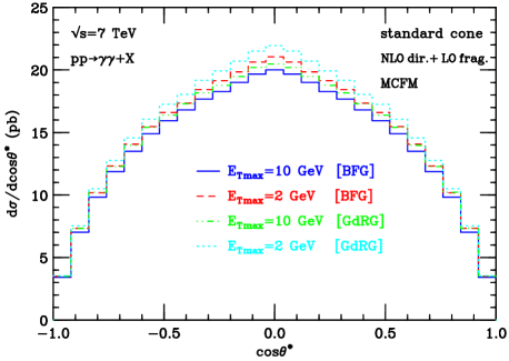
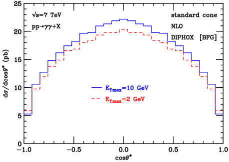
Figure 9: The $\cos~{}\theta^{*}$ differential cross section for standard cone isolation with two different values of $E_{T\,{\rm max}}$ (2 GeV and 10 GeV) and the same photon kinematical cuts as in Fig. 4. The QCD results are obtained at the central value of the scales ($\mu_{F}=\mu_{R}=\mu_{frag}=\mu_{0}\equiv M_{\gamma\gamma}$). The results with NLO direct + LO fragmentation components (left panel) use BFG and GdRG_LO fragmentation functions. The NLO results (right panel) use BFG fragmentation functions.

We interpret the unphysical dependence on $E_{T\,{\rm max}}$ of the MCFM results as the effect of a mismatch between the perturbative orders in the direct and fragmentation components. Indeed the $E_{T\,{\rm max}}$ dependence of the MCFM results is mostly produced by the NLO corrections to the direct component through the partonic subprocess $qg\rightarrow q\gamma\gamma$ at the tree level. The tree-level contribution of this partonic subprocess is formally positive definite and, as such, it would lead to an increasing (physical) dependence on $E_{T\,{\rm max}}$ by increasing $E_{T\,{\rm max}}$. However, this contribution is divergent in the phase space region where the final-state $q$ is collinear to one of the produced photons. The collinear divergence (which is in turn absorbed and factorized in the non-perturbative definition of the quark-to-photon fragmentation function) is removed through its subtraction (which is actually performed in the ${\overline{\rm MS}}$ factorization scheme [31]) from the direct component contribution at NLO. Since the collinear-divergent term that is subtracted is formally positive definite, the final NLO correction to the direct component is finite but it is not necessarily positive definite and, consequently, it can have an unphysical dependence on $E_{T\,{\rm max}}$ (this unphysical dependence is actually also visible in the direct component of the NLO results in Table 1). It turns out that the result of the calculation with NLO direct + LO fragmentation components has an unphysical dependence on $E_{T\,{\rm max}}$.

In the case of the complete NLO result for standard isolation, the NLO corrections to the fragmentation component (corrections to both the partonic cross sections and the scale evolution of the fragmentation functions) are consistently (at the formal level) included within the ${\overline{\rm MS}}$ factorization scheme. Although these corrections are not particularly sizeable in absolute terms, their inclusion leads to NLO results with a qualitative dependence on $E_{T\,{\rm max}}$ that agrees with physical expectation.

In the context of smooth isolation, the entire $E_{T\,{\rm max}}$ dependence at NLO is due to partonic subprocesses with two photons and a parton in the final state, which are evaluated at the tree level. The contribution of these tree-level subprocesses is positive definite (with no collinear divergences to be subtracted) and it cannot produce any unphysical dependence on $E_{T\,{\rm max}}$: NLO smooth isolation cross sections cannot decrease by increasing $E_{T\,{\rm max}}$. Incidentally, we note that this elementary reasoning, based on positivity, cannot be applied at the NNLO, since the $E_{T\,{\rm max}}$ dependence at NNLO receives contributions from both tree-level and loop-level partonic processes. Nonetheless, as shown in Sect. 3.3 (see Fig. 16 and the accompanying comments) the NNLO results for smooth isolation do not show unphysical dependence on $E_{T\,{\rm max}}$.

As anticipated in our comments on the results in Fig. 3, we present a more detailed discussion on the differential cross section $d\sigma/dM_{\gamma\gamma}$ in the region where $M_{\gamma\gamma}$ is close to the LO threshold ($M_{\gamma\gamma}\sim M^{LO}$). The numerical results in Fig. 3 are obtained by using a (constant) bin size of 2 GeV in $M_{\gamma\gamma}$. To quantitatively examine the detailed shape of $d\sigma/dM_{\gamma\gamma}$, we perform the numerical calculation with a finer resolution in $M_{\gamma\gamma}$ and we use $M_{\gamma\gamma}$ bins with a constant size of 0.1 GeV (which is 20 times smaller than that used in Fig. 3). The results of the calculation for smooth isolation at both LO and NLO are presented in Fig. 10. Specifically, we use $E_{T\,{\rm max}}=10$ GeV and, at each perturbative order, we report the two results with the scale choices $\{\mu_{R}=M_{\gamma\gamma}/2,\mu_{F}=2M_{\gamma\gamma}\}$ and $\{\mu_{R}=2M_{\gamma\gamma},\mu_{F}=M_{\gamma\gamma}/2\}$ (the region enclosed by these two scale-dependent results corresponds to the scale variation band in Fig. 3). We remark that the smooth isolation results in Fig. 10 exactly refer to the same quantity (and to the same theoretical setup) as the corresponding results in Fig. 3-right, the only difference being the much smaller $M_{\gamma\gamma}$ bin size used in Fig. 10. Various shape details that are visible in Fig. 10 disappear in Fig. 3 since they are smeared by the larger bin size.

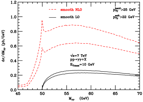
Figure 10: The differential cross section $d\sigma/dM_{\gamma\gamma}$ for smooth isolation with $E_{T\,{\rm max}}=10$ GeV and the same kinematical cuts as in Fig. 3. The LO (black solid) and NLO (red dashed) numerical results use $M_{\gamma\gamma}$ bins with constant size of 0.1 GeV. At both perturbative orders, the maximum and minimum values of $d\sigma/dM_{\gamma\gamma}$ correspond to the scale choices $\{\mu_{R}=M_{\gamma\gamma}/2,\mu_{F}=2M_{\gamma\gamma}\}$ and $\{\mu_{R}=2M_{\gamma\gamma},\mu_{F}=M_{\gamma\gamma}/2\}$, respectively.

We note that the qualitative shape of $d\sigma/dM_{\gamma\gamma}$ in Fig. 10 is independent of the scale choice, which only affects the size of $d\sigma/dM_{\gamma\gamma}$. The behaviour of the LO result has been discussed in the paragraph below Eq. (18). The LO result has a threshold at $M_{\gamma\gamma}=M^{LO}_{\rm dir}=50$ GeV and, close to the threshold, it vanishes as

$$\frac{d\sigma^{LO}_{\rm smooth}}{dM_{\gamma\gamma}}\propto{\sqrt{\epsilon_{M}}}\;\;\Theta(M_{\gamma\gamma}-M^{LO}_{\rm dir})\;\;,\quad\quad\quad(M_{\gamma\gamma}\sim M^{LO}_{\rm dir})\;,$$ (34)

where $\epsilon_{M}=|1-(M_{\gamma\gamma}/M^{LO}_{\rm dir})|$. The threshold and the square-root behaviours near threshold are visible in the LO results of Fig. 10. At the NLO, $d\sigma/dM_{\gamma\gamma}$ is not vanishing at $M_{\gamma\gamma}=M^{LO}_{\rm dir}$ (the threshold disappears) and it has a cusp behaviour in the vicinity of the LO threshold. Following the general analysis in Ref. [60], we have examined the NLO shape of $d\sigma/dM_{\gamma\gamma}$ at $M_{\gamma\gamma}\sim M^{LO}_{\rm dir}$ in analytic form and we find the dominant behaviour

$$\frac{d\sigma^{NLO}_{\rm smooth}}{dM_{\gamma\gamma}}=a_{0}-{\sqrt{\epsilon_{M}}}\left[a_{(-)}\,\ln\left(\frac{1}{\epsilon_{M}}\right)\Theta(M^{LO}_{\rm dir}-M_{\gamma\gamma})+a_{(+)}\,\ln^{2}\left(\frac{1}{\epsilon_{M}}\right)\Theta(M_{\gamma\gamma}-M^{LO}_{\rm dir})\right]+\;\;\dots\;\;,$$ (35)

where $a_{0},a_{(-)}$ and $a_{(+)}$ are positive constants (i.e., they do not depend on $M_{\gamma\gamma}$) and the dots on the right-hand side denote subdominant contributions (terms that are relatively suppressed by powers of $(\ln\epsilon_{M})^{-1}$ or ${\sqrt{\epsilon_{M}}}\,$) in the limit $M_{\gamma\gamma}\rightarrow M^{LO}_{\rm dir}$. In particular, Eq. (35) implies that the first derivative of $d\sigma/dM_{\gamma\gamma}$ with respect to $M_{\gamma\gamma}$ (i.e., the slope of $d\sigma/dM_{\gamma\gamma}$) diverges to $+\infty$ ($-\infty$) if $M_{\gamma\gamma}\rightarrow M^{LO}_{\rm dir}$ from below (above) the LO threshold. This slope leads to the double-side cusp of Fig. 10.

At low values of $M_{\gamma\gamma}$ in Fig. 10, $d\sigma^{NLO}/dM_{\gamma\gamma}$ is very small. Its value starts to rapidly increase at $M_{\gamma\gamma}\sim 47$ GeV. This confirms the observation in our previous comments on the NLO result in Figs. 3 and 6: although $d\sigma/dM_{\gamma\gamma}$ has no physical threshold, it displays an ‘approximate’ threshold behaviour at $M_{\gamma\gamma}\sim M^{LO}\simeq 47$ GeV (see Eq. (22)) since the kinematical region where $M_{\gamma\gamma}\raisebox{-2.58334pt}{\hbox to0.0pt{$\,\sim\,$\hss}}\raisebox{1.72218pt}{$\,<\,$}M^{LO}$ receives contributions only from physical events in which the diphoton pair is accompanied by hard (high transverse momentum) parton radiation in the final state (see Eq. (23) and related comments). At high values of $M_{\gamma\gamma}$ in Fig. 10, the shape of the LO and NLO results is quite similar. In particular, the position of the (broad) peak of $d\sigma/dM_{\gamma\gamma}$ (at $M_{\gamma\gamma}\sim 57$ GeV) does not substantially vary in going from the LO to the NLO results.

Considering the NLO result with the scale configuration $\{\mu_{R}=M_{\gamma\gamma}/2,\mu_{F}=2M_{\gamma\gamma}\}$ in Fig. 10, we also notice that the value of $d\sigma/dM_{\gamma\gamma}$ at $M_{\gamma\gamma}=M^{LO}_{\rm dir}$ (i.e., the height of the cusp) is quite large and, in particular, it is larger than the value in the peak region at $M_{\gamma\gamma}\sim 57$ GeV. Independently of the scale configuration, we observe that the cusp behaviour is located in a tiny region of $M_{\gamma\gamma}$ around $M_{\gamma\gamma}=M^{LO}_{\rm dir}$ and, consequently, such behaviour quantitatively disappears by increasing the bin size in $M_{\gamma\gamma}$ (see Fig. 3).

The shape of $d\sigma^{NLO}/dM_{\gamma\gamma}$ at $M_{\gamma\gamma}\sim M^{LO}_{\rm dir}$ (Fig. 10 and Eq. (35)) is definitely unphysical and it deserves additional comments. This shape (and the expression in Eq. (35)) follows from the general discussion and results of Ref. [60]. According to Ref. [60], an observable that has a discontinuity at some point $x=x_{0}$ (inside the physical region) at the LO necessarily has a logarithmic divergent (though integrable) discontinuity at the same point at the NLO. In our specific case, the slope of $d\sigma^{LO}/dM_{\gamma\gamma}$ has a discontinuity at $M_{\gamma\gamma}=M^{LO}_{\rm dir}$ (though $d\sigma^{LO}/dM_{\gamma\gamma}$ is continuous at the same point): therefore, the slope of $d\sigma^{NLO}/dM_{\gamma\gamma}$ has a logarithmically-enhanced discontinuity (see Eqs. (34) and (35)) at $M_{\gamma\gamma}=M^{LO}_{\rm dir}$ (though $d\sigma^{NLO}/dM_{\gamma\gamma}$ remains continuous at the same point).

The logarithmic enhancement of the discontinuity is due to soft-gluon radiation at the NLO [60]. In our specific case, the relevant NLO partonic processes are the real emission contribution

$$q{\bar{q}}\rightarrow\gamma\gamma g$$ (36)

at the tree level (here, the final-state gluon is soft and collinear to one of the initial-state partons), and the virtual contribution to $q{\bar{q}}\rightarrow\gamma\gamma$ at the one-loop level. A non-smooth kinematical mismatch (such as that produced by a discontinuous observable) between the real and virtual contributions produces the logarithmic enhancement [60]. In our specific case, the NLO virtual process $q{\bar{q}}\rightarrow\gamma\gamma$ still fulfils the same kinematical constraints as at the LO (in particular, transverse-momentum conservation implies $p_{T\gamma}^{soft}=p_{T\gamma}^{hard}\geq p_{H}=25$ GeV, independently of the value of $p_{S}$) and, consequently, it only contributes at $M_{\gamma\gamma}\geq M^{LO}_{\rm dir}$. In contrast, the soft gluon radiated in the process of Eq. (36) produces diphoton events with $M_{\gamma\gamma}<M^{LO}_{\rm dir}$, since the softer photon absorbs the soft-gluon momentum recoil thus decreasing its transverse momentum $p_{T\gamma}^{soft}$ below its LO kinematical limit (i.e., we have $p_{T\gamma}^{soft}<p_{H}\leq p_{T\gamma}^{hard}$, although $p_{T\gamma}^{soft}\geq p_{S}$). It follows that real soft-gluon radiation is completely unbalanced by virtual radiation in the region just below the LO threshold, and this produces the corresponding logarithmically-enhanced cusp at $M_{\gamma\gamma}<M^{LO}_{\rm dir}$ in Fig. 10 and Eq. (35). Therefore, the shape of $d\sigma^{NLO}/dM_{\gamma\gamma}$ just below the LO threshold is exactly a consequence of the reasoning and results of Ref. [60]. Instead, the logarithmic enhancement of the slope of $d\sigma^{NLO}/dM_{\gamma\gamma}$ just above the LO threshold ($M_{\gamma\gamma}>M^{LO}_{\rm dir}$) can be somehow regarded as a corollary to the reasoning in Ref. [60]. Both real and virtual terms contribute above the threshold, but here the slope of $d\sigma/dM_{\gamma\gamma}$ is already divergent (see Eq. (34)), and not only discontinuous, at the LO: this LO divergent behaviour produces a strong real–virtual mismatch and an ensuing logarithmic enhancement at the NLO (see Fig. 10 and Eq. (35)).

The unphysical cusp behaviour of $d\sigma^{NLO}/dM_{\gamma\gamma}$ at $M_{\gamma\gamma}\sim M^{LO}_{\rm dir}$ occurs for both smooth and standard isolation (although Fig. 10 only shows smooth isolation results). Indeed, the LO direct component of the standard isolation result exactly coincides with the LO smooth isolation result and, therefore, the NLO soft-gluon radiative correction to the direct component for standard isolation exactly behaves in the same way as we have just described for the smooth isolation criterion. In contrast, the NLO radiative corrections to the fragmentation component do not produce a cusp behaviour in the vicinity of the corresponding LO threshold at $M_{\gamma\gamma}\sim M^{LO}_{\rm frag}$ ($M^{LO}_{\rm frag}=M^{LO}\simeq 47$ GeV in Fig. 10). This follows from the fact that $d\sigma^{LO}_{\rm frag}/dM_{\gamma\gamma}$ is sufficiently smooth at $M_{\gamma\gamma}\sim M^{LO}_{\rm frag}$ (see the discussion at the end of Sect. 2.3.2) and, in particular, the slope of $d\sigma^{LO}_{\rm frag}/dM_{\gamma\gamma}$ is not discontinuous (it actually vanishes) at $M_{\gamma\gamma}=M^{LO}_{\rm frag}$. Obviously, the NLO fragmentation component contributes to $d\sigma^{NLO}/dM_{\gamma\gamma}$ at $M_{\gamma\gamma}\sim M^{LO}_{\rm dir}$, but its contribution is smooth and it only produces a finite vertical displacement of the cusp of the NLO direct component.

The unphysical shape (i.e., the cusp behaviour) of $d\sigma/dM_{\gamma\gamma}$ at NLO persists at each subsequent perturbative order. Such an unphysical fixed-order behaviour can be removed by a proper all-order resummation of soft-gluon effects [60]. Resummation leads to a smooth behavior (Sudakov shoulder) [60] of both $d\sigma/dM_{\gamma\gamma}$ and its slope from the peak region at $M_{\gamma\gamma}\sim 57$ GeV to the ‘approximate’ threshold at $M_{\gamma\gamma}\sim 47$ GeV.

In the context of fixed-order computations, the unphysical behaviour produces perturbative instabilities that can be reduced only by considering observables that are sensitive to a ‘sufficiently-smeared’ region in the vicinity of $M_{\gamma\gamma}\sim M^{LO}_{\rm dir}$. The degree of ‘sufficient’ smearing or insensitivity depends on various factors, such as the type of observable, the bin size and the kinematical cuts. We briefly comments on these factors. As for the dependence on the observable, the total cross section has little sensitivity to these instabilities, the differential cross section $d\sigma/d\cos\theta^{*}$ at central values of $cos\theta^{*}$ has some sensitivity, and the differential cross section $d\sigma/dM_{\gamma\gamma}$ in the region close to $M^{LO}_{\rm dir}$ is certainly sensitive. The bin size dependence is obvious at the qualitative level, but it is less obvious at the quantitative level. A sufficiently-large $M_{\gamma\gamma}$-bin at $M_{\gamma\gamma}\sim M^{LO}_{\rm dir}$ removes the cusp behaviour, but it leads to a binned value of $d\sigma/dM_{\gamma\gamma}$ that depends on the bin size and also on the average slope of $d\sigma/dM_{\gamma\gamma}$ in the region close to the LO threshold (a larger value of the average slope increases the sensitivity to the bin size). In our discussion on the results in Fig. 3, we have argued that $d\sigma^{NLO}/dM_{\gamma\gamma}$ is possibly sensitive to the perturbative instabilities even if the $M_{\gamma\gamma}$-bin size is 2 GeV. The dependence on the $p_{T}$ cuts has been pointed out in our comments on the results in Fig. 6, where we have observed that the size of the perturbative instabilities can be affected by the average slope of $d\sigma/dM_{\gamma\gamma}$ at $M_{\gamma\gamma}\sim M^{LO}_{\rm dir}$, which directly depends on the difference between $M^{LO}_{\rm dir}$ and $M^{LO}$ (i.e., on the values of the $p_{T}$ cuts $p_{H}$ and $p_{S}$). Certainly, the relevance of these perturbative instabilities also depends on the required theoretical accuracy of the QCD calculation. In Sect. 3.5 we present additional results and comments on this kind [60] of instabilities and related observables.

3 Diphoton production at the LHC and NNLO results

In this section we consider diphoton production in $pp$ collisions at LHC energies and we present perturbative QCD results at the NNLO. We use smooth cone isolation since the NNLO calculation for standard cone isolation has not yet been performed. Within smooth isolation, we also present corresponding results at LO and NLO to directly comment on features of the perturbative QCD expansion.

In Ref. [35] we presented NNLO results for diphoton production at the LHC in diphoton kinematical configurations that are typically used in the context of Higgs boson searches and studies. In particular, we considered the region $M_{\gamma\gamma}<200$ GeV and highly-asymmetric cuts on the photon transverse momenta (i.e., $p_{T}^{hard}>40$ GeV, $p_{T}^{soft}>25$ GeV). In the following we consider different kinematical configurations and we discuss various aspects of the NNLO results. Diphoton production results at NNLO and comparisons with LHC data are also presented in Refs. [4, 7, 8, 37]. NNLO results for diphoton production in $pp$ collisions at ${\sqrt{s}}=100$ TeV are presented in Ref. [97] (see Sect. 8.3 therein).

In our computation the radius of the photon isolation cone is set at the value $R=0.4$. We use the smooth isolation function $\chi(r;R)$ in Eq. (3) (the same form of the isolation function is used in the NNLO results reported in Refs. [4, 7, 8]) and the value of the power $n$ is set to $n=1$ for most of the results, although we comment on the $n$ dependence of total cross sections and of some differential cross sections.

The QCD results are obtained by using the programs 2$\gamma$NNLO and MATRIX. The theoretical setup of our calculation is the same as described at the beginning of Sect. 2.3 (in particular, we use the value $\alpha=1/137$ of the QED coupling constant and the MMHT 2014 sets [91] of PDFs). The only difference with respect to Sect. 2.3 regards the central value $\mu_{0}$ of the renormalization ($\mu_{R}$) and factorization ($\mu_{F}$) scales. Unlike the case of Sect. 2.3 (where $\mu_{0}=M_{\gamma\gamma}$), throughout this section we use the dynamical central value $\mu_{0}=\sqrt{{M_{\gamma\gamma}}^{2}+p^{2}_{T\gamma\gamma}}=M_{T\gamma\gamma}$ ($M_{T\gamma\gamma}$ is the transverse mass of the diphoton system), which also depends on the transverse momentum $p_{T\gamma\gamma}$ of the photon pair. We consider independent scale variations of $\mu_{R}$ and $\mu_{F}$ within the ranges $0.5\leq\mu_{R}/\mu_{0}\leq 2$ and $0.5\leq\mu_{F}/\mu_{0}\leq 2$ around the central value $\mu_{0}$. Practically, we obtain the results for nine scale configurations (we independently combine $\mu_{R}/\mu_{0}=\{0.5,1,2\}$ and $\mu_{F}/\mu_{0}=\{0.5,1,2\}$) and we evaluate scale uncertainties by considering the maximum value and minimum value among these results. We have checked that, for most of the computed quantities (including total cross sections), the maximum and minimum values correspond to the scale configurations $\{\mu_{R}=\mu_{0}/2$, $\mu_{F}=2\mu_{0}\}$ and $\{\mu_{R}=2\mu_{0}$ , $\mu_{F}=\mu_{0}/2\}$, respectively.

The bulk of the diphoton cross section is produced at small values of $p_{T\gamma\gamma}$ ($p_{T\gamma\gamma}\ll M_{\gamma\gamma}$). Therefore, to the purpose of computing the total cross section, the choice of the dynamical scale $\mu_{0}=M_{T\gamma\gamma}$ leads to results that are basically similar to those obtained with the scale choice $\mu_{0}\sim M_{\gamma\gamma}$. The dynamical scale $\mu_{0}=M_{T\gamma\gamma}$ sizeably differs from the diphoton invariant mass $M_{\gamma\gamma}$ only at high values of $p_{T\gamma\gamma}$ (i.e., in the kinematical regions where $M_{\gamma\gamma}\ll p_{T\gamma\gamma}$). High values of $p_{T\gamma\gamma}$ can be reached either in the highly unbalanced regime where $p_{T\gamma}^{soft}\ll p_{T\gamma}^{hard}$ or in the highly boosted regime where the two photons have comparable transverse momenta ($p_{T\gamma}^{soft}\sim p_{T\gamma}^{hard}$) and small values of both the azimuthal angle separation $\Delta\Phi_{\gamma\gamma}$ and the rapidity separation $\Delta y_{\gamma\gamma}$. In both these regimes, $p_{T\gamma\gamma}$ is balanced by a recoiling high-$p_{T}$ jet, and the dynamical scale $\mu_{0}=M_{T\gamma\gamma}\sim p_{T\gamma\gamma}$ parametrically mimics the scale of the invariant mass $M_{\gamma\gamma jet}$ ($p_{T\gamma\gamma}\sim{\cal O}(M_{\gamma\gamma jet})$) of the diphoton+jet final-state system, which is the characteristic scale of the underlying hard-scattering subprocesses.

In this paper we do not evaluate PDF uncertainties. NLO PDF uncertainties at the LHC are computed in the diphoton studies of Refs. [4, 7, 8] and combined with scale variation uncertainties (PDF uncertainties are found to be typically smaller than scale uncertainties). In Ref. [7] the PDF uncertainty on the NLO total cross section is explicitly quoted and it amounts to about $\pm 5$%. The PDF uncertainties that are computed in Ref. [8] are at the level of $\pm 2$%.

As main reference kinematical configuration we consider LHC collisions at the centre–of–mass energy $\sqrt{s}=7$ TeV and we use the kinematical acceptance cuts implemented by the ATLAS Collaboration in the analysis of Ref. [4]. We require $p_{T}^{hard}\geq 25$ GeV and $p_{T}^{soft}\geq 22$ GeV, we restrict the rapidity of both photons to the regions $|y_{\gamma}|<1.37$ and $1.52<|y_{\gamma}|\leq 2.37$, and the minimum angular separation between the two photons is $R_{\gamma\gamma}^{\rm min}=0.4$. These acceptance cuts coincide with the main reference cuts in Sect. 2.3, apart from the exclusion of the rapidity interval $1.37<|y_{\gamma}|<1.52$. The ATLAS data are selected by using standard cone isolation with the isolation parameters $R=0.4$ and $E_{T\,{\rm max}}=4~{}$GeV. We use smooth cone isolation with $R=0.4$ and $E_{T\,{\rm max}}=4~{}$GeV. All the results in this section refer to this configuration and to this value of $E_{T\,{\rm max}}$, unless otherwise explicitly stated.

3.1 Total cross sections

The results of the LO, NLO and NNLO total cross sections are reported in Table 2.

At the LO the value of the total cross section is $\sigma^{LO}=9.293~{}{\rm pb}~{}^{+10.9\,{\%}}_{-11.9\,{\%}}$ (scale), and it does not depend on the power $n$ of the isolation function in Eq. (3). At the NLO with $n=1$ we have $\sigma^{NLO}=28.55~{}{\rm pb}~{}^{+12.5\,{\%}}_{-12.2\,{\%}}$ (scale). The features of these LO and NLO results are very similar to those of the smooth isolation results presented in Sect. 2.3.1 (see Table 1), apart from an overall reduction (by roughly 10%) of the cross section values, which is due to the exclusion of the photon rapidity region $1.37<|y_{\gamma}|<1.52\,$.

	$\sigma^{{\rm LO}}$  (pb)	$\sigma^{{\rm NLO}}$  (pb)	$\sigma^{{\rm NNLO}}$  (pb)
$n$ ind.	$9.293~{}^{+10.9\,{\%}}_{-11.9\,{\%}}$
$n=0.5$		$29.40~{}^{+12.8\,{\%}}_{-12.4\,{\%}}$	$40.98(68)~{}^{+8.3\,{\%}}_{-8.7\,{\%}}$
$n=1$		$28.55~{}^{+12.5\,{\%}}_{-12.2\,{\%}}$	$39.50(50)~{}^{+7.9\,{\%}}_{-8.4\,{\%}}$
$n=2$		$27.98~{}^{+12.3\,{\%}}_{-11.9\,{\%}}$	$37.53(52)~{}^{+7.0\,{\%}}_{-7.8\,{\%}}$

Table 2: Results for LO, NLO and NNLO total cross sections with the photon kinematical cuts described in the text (beginning of Sect. 3). The results are obtained by using smooth isolation and $n$ denotes the power in the isolation function of Eq. (3). The central values of $\sigma$ are obtained with the scale choice $\mu_{R}=\mu_{F}=\mu_{0}=M_{T\gamma\gamma}$, and the scale dependence corresponds to independent variations of $\mu_{R}$ and $\mu_{F}$ between $\mu_{0}/2$ and $2\mu_{0}$. The last digit of the LO and NLO cross section values has an error of one unit from the statistical uncertainty of the numerical calculation. The systematical error on $\sigma^{NNLO}$ is explicitly given in round brackets.

The value of the NNLO total cross section with $n=1$ is $\sigma^{NNLO}=39.50~{}{\rm pb}~{}^{+7.0\,{\%}}_{-7.8\,{\%}}$ (scale). This result is obtained by using MATRIX with the default setup [41]. The value of the NNLO cross section is obtained by the code through an $r_{\rm cut}\rightarrow 0$ extrapolation of the $r_{\rm cut}$ dependence for $r_{\rm cut}>0.15\%$. The systematic uncertainty of the extrapolated result, as explicitly reported in Table 2, is at the $\pm{\cal O}(1\%)$ level. Such uncertainty is much smaller than the NNLO perturbative uncertainties, and thus still acceptable to the purpose of the present paper. More accurate results could in principle be obtained with MATRIX by using the option switch_qt_accuracy=1, which lowers the value of the minimum $r_{\rm cut}$ down to $0.05\%$. The MATRIX result is in agreement with the corresponding result obtained by using 2$\gamma$NNLO within the systematical uncertainties.

We have computed the $n$ dependence of the total cross section in the range $0.5\leq n\leq 2$ (see Table 2). At the NNLO (NLO) we find that the result with $n=1$ increases by about 4% (3%) with $n=0.5$ and decreases by about 5% (2%) with $n=2$. At both NLO and NNLO we note that this $n$ dependence of the total cross section is monotonic and in qualitative agreement with the physical expectation in Eq. (8). In particular, we point out that the $n$ dependence of the cross section increases (especially at $n=2$) in going from NLO to NNLO: the NNLO results are more sensitive to the value of $n$. We also note that variations of $n$ in the interval $0.5\leq n\leq 2$ produce (at both NLO and NNLO) variations of the total cross section that are smaller than those produced by the scale dependence at fixed $n$. In view of this, we limit ourselves to using $n=1$ (unless otherwise stated) for most of our subsequent studies.

Throughout this section we present explicit results on the contribution of the different initial-state partonic channels to various observables at the NNLO. To simplify the presentation we consider the partition of the total result in three contributions: the contribution of the $gg$ partonic channel (and its partial component from the box contribution $gg\rightarrow\gamma\gamma$), the contribution of the $qg+{\bar{q}}g$ partonic channel (it is dominated by its $qg$ component and it is briefly labelled as $qg$ channel) and the contribution of the remaining partonic channels (this contribution is dominated by the $q{\bar{q}}$ initial state and it is briefly labelled as $q{\bar{q}}$ channel). This decomposition in partonic channels has a mild scale dependence and we always present results at the central values $\mu_{R}=\mu_{F}=\mu_{0}=M_{T\gamma\gamma}$ of the scales.

About 9% of $\sigma^{NNLO}$ is due to the $gg$ channel. Therefore, the contribution of the $gg$ channel at NNLO is not sizeable (it is quantitatively comparable to the size of the scale dependence of $\sigma^{NNLO}$), despite the fact that the contribution of the box $gg\rightarrow\gamma\gamma$ is approximately equal to one half of the LO total cross section. We also note that the total $gg$ contribution at NNLO is partly smaller than its box component: the additional NNLO contributions from $gg$ collisions turn out to be negative and have an absolute size that is approximately one quarter of the box contribution. The NNLO result for the total cross section is dominated by the $qg$ and $q{\bar{q}}$ channels, which approximately equally contribute to $\sigma^{NNLO}$. The NNLO cross section receives contributions of about 48% from the $q{\bar{q}}$ channel and of about 43% from the $qg$ channel.

The NLO total cross section is roughly 3 times larger than $\sigma^{LO}$. The NNLO $K$ factor, $K^{NNLO}=\sigma^{NNLO}/\sigma^{NLO}$, at central values of the scales is $K^{NNLO}\simeq 1.4$. We see that both NLO and NNLO corrections are sizeable. The large size of the QCD radiative corrections up to NNLO is justifiable and understandable following and extending the reasoning that we have presented in Sect. 2.3.1 (see Eqs. (9) and (11) and accompanying comments). At the LO only the $q{\bar{q}}$ channel contributes. At the NLO, $\sigma^{NLO}$ receives contribution also from the $qg$ channel. The relative NLO correction from the $qg$ channel is of the order of $\alpha_{\mathrm{S}}\,{\cal L}_{qg}/{\cal L}_{q{\bar{q}}}$ and the large value of the PDF luminosity ratio ${\cal L}_{qg}/{\cal L}_{q{\bar{q}}}$ compensates the suppression factor produced by $\alpha_{\mathrm{S}}$. Therefore, the presence of a new NLO partonic channel, the $qg$ channel, with a large PDF luminosity implies that, at the quantitative level, there is no parametric hierarchy of ${\cal O}(\alpha_{\mathrm{S}})$ between NLO corrections and LO result. As a consequence, the NLO result has to be quantitatively regarded as an effective lowest-order estimate of the cross section. The next-order corrections to this result are parametrically of ${\cal O}(\alpha_{\mathrm{S}})$ (the contribution of the new $gg$ channel at NNLO is not particularly sizeable) and they turn out to have a ‘moderate’ size. Indeed, the value $K^{NNLO}\simeq 1.4$ has a size that is not much different from the typical (and expected) size of NLO $K$ factors for various hard-scattering processes at hadron colliders. We also note that the scale dependence of the total cross section is partly reduced in going from NLO to NNLO (it is not so in going from LO to NLO). However, we remark that the values of $\sigma^{NNLO}$ and $\sigma^{NLO}$ do not overlap by including their corresponding scale dependence. This implies that the computed scale dependence of $\sigma^{NNLO}$ cannot be consistently regarded as a reliable estimate of uncalculated radiative corrections to the total cross section. The ‘true’ theoretical uncertainty of $\sigma^{NNLO}$ due to higher-order corrections is certainly larger than the NNLO scale dependence that we have computed.

3.2 Differential cross sections

We now move to consider kinematical distributions. In particular, we consider the differential cross sections $d\sigma/dM_{\gamma\gamma},d\sigma/d\cos\theta^{*},d\sigma/d\Delta\Phi_{\gamma\gamma}$ and $d\sigma/dp_{T\gamma\gamma}$, which are also considered in Ref. [4], and we use the same kinematical bins as used for the corresponding experimental data in Tables 2–5 of Ref. [4].

The LO, NLO and NNLO results (including their scale dependence) for $d\sigma/dM_{\gamma\gamma}$ are presented in the main panel of Fig. 11-left. In the lower panel of Fig. 11-left we present the NNLO $K$ factor and the relative scale dependence at NLO.

The NNLO $K$ factor is defined as

$$K^{NNLO}(x)=\frac{d\sigma^{NNLO}(\mu)/dx}{d\sigma^{NLO}(\mu_{0})/dx}\;\;,$$ (37)

where $d\sigma^{NNLO}(\mu)/dx$ is the scale dependent NNLO result for the differential cross section $d\sigma/dx$ with respect to the kinematical variable $x$, and $d\sigma^{NLO}(\mu_{0})/dx$ is the corresponding NLO result at central scales ($\mu_{R}=\mu_{F}=\mu_{0}=M_{T\gamma\gamma}$). The relative scale dependence at NLO is defined as

$$\frac{d\sigma^{NLO}(\mu)/dx}{d\sigma^{NLO}(\mu_{0})/dx}\;\;,$$ (38)

where $d\sigma^{NLO}(\mu)/dx$ is the scale dependent NLO result.

The comparisons between the numerical values of the quantities in Eqs. (37) and (38) gives a direct quantitative illustration of the degree of overlap (including scale dependencies) of the NNLO and NLO results. By inspection of Fig. 11-left we see that the two bands in the lower panel do not overlap. This lack of overlap has already been observed for the case of the NNLO and NLO total cross sections and the same qualitative features will be observed for the differential cross sections $d\sigma/d\cos\theta^{*},d\sigma/d\Delta\Phi_{\gamma\gamma}$ and $d\sigma/dp_{T\gamma\gamma}$ that we present in the following.

As we have already remarked, this implies that the ‘true’ perturbative uncertainty of the NNLO result for these observables is larger than the corresponding NNLO scale dependence that we explicitly compute.

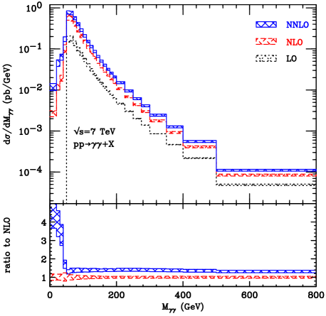
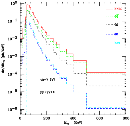
Figure 11: The differential cross section $d\sigma/dM_{\gamma\gamma}$ with the same photon kinematical cuts as in Table 2. The main panel in the left-hand side shows the LO (black dotted), NLO (red dashed) and NNLO (blue solid) results, with the corresponding scale dependence. The lower subpanel presents the NNLO $K$ factor (including its scale dependence) and the relative scale dependence at NLO. The panel in the right-hand side shows the NNLO result at central scales and its decomposition in the contributions of different initial-state partonic channels: $q{\bar{q}}$ (green dot-dashed), $qg$ (black dotted) and $gg$ (blue dashed). The separate contribution of the box $gg\rightarrow\gamma\gamma$ squared amplitude is also shown (light-blue dot-dot-dashed).

A minor comment on the results in Fig. 11 regards the first bin, where $0\leq M_{\gamma\gamma}\leq 20$ GeV. As discussed in Sect. 2.3.3 (see, in particular the comments that accompany Eq. (23)), the differential cross section $d\sigma/dM_{\gamma\gamma}$ in Fig. 11 has the lower kinematical limit $M_{\gamma\gamma}\raisebox{-2.58334pt}{\hbox to0.0pt{$\,\sim\,$\hss}}\raisebox{1.72218pt}{$\,>\,$}10$ GeV. This implies that we do not actually compute $d\sigma/dM_{\gamma\gamma}$ with $M_{\gamma\gamma}\rightarrow 0$. It also implies that the rapid decrease of $d\sigma/dM_{\gamma\gamma}$ from the second to the first bin is partly an artifact of the vanishing of $d\sigma/dM_{\gamma\gamma}$ in the region where $M_{\gamma\gamma}\raisebox{-2.58334pt}{\hbox to0.0pt{$\,\sim\,$\hss}}\raisebox{1.72218pt}{$\,<\,$}10$ GeV (this region covers about one half of the first bin). Obviously the same kinematical artifact equally affects the experimental data in the first bin (the artifact has no effect on the comparison between data and theory and on the quantities in the lower panel of Fig. 11-left).

The main features of $d\sigma/dM_{\gamma\gamma}$ and of the corresponding LO and NLO results are discussed in Sects. 2.3.2 and 2.3.3 (see, in particular, Fig. 3 and related comments). That discussion also includes some comments on our expectations about the NNLO results. As noticed below, those expectations are confirmed by the NNLO results in Fig. 11.

The presence of the (unphysical) LO threshold at $M_{\gamma\gamma}=50$ GeV is responsible for the shape of $d\sigma/dM_{\gamma\gamma}$ in Fig. 11. The two invariant-mass bins ($40~{}{\rm GeV}\leq M_{\gamma\gamma}\leq 50~{}{\rm GeV}$ and $50~{}{\rm GeV}\leq M_{\gamma\gamma}\leq 60~{}{\rm GeV}$) that are closest to the LO threshold have a relatively-large size, which does not offer enough resolution to examine the detailed shape of $d\sigma/dM_{\gamma\gamma}$ at $M_{\gamma\gamma}\sim 50$ GeV. Therefore, we simply comment on the high-mass ($M_{\gamma\gamma}\raisebox{-2.58334pt}{\hbox to0.0pt{$\,\sim\,$\hss}}\raisebox{1.72218pt}{$\,>\,$}50$ GeV) and low-mass ($M_{\gamma\gamma}\raisebox{-2.58334pt}{\hbox to0.0pt{$\,\sim\,$\hss}}\raisebox{1.72218pt}{$\,<\,$}50$ GeV) regions (comments on the region that is very close to $M_{\gamma\gamma}=50$ GeV are postponed to Sect. 3.5).

In the high-mass region, the NLO and NNLO corrections to $d\sigma/dM_{\gamma\gamma}$ have a size that is similar to that of the corresponding results for the total cross section. The value of $K^{NNLO}(M_{\gamma\gamma})$ (including its scale dependence) for $d\sigma/dM_{\gamma\gamma}$ is very similar to the corresponding NNLO $K$ factor for the total cross section. In particular, $K^{NNLO}(M_{\gamma\gamma})$ is remarkably independent of $M_{\gamma\gamma}$: we have $K^{NNLO}(M_{\gamma\gamma})\simeq 1.4$ for $50~{}{\rm GeV}\raisebox{-2.58334pt}{\hbox to0.0pt{$\,\sim\,$\hss}}\raisebox{1.72218pt}{$\,<\,$}M_{\gamma\gamma}\raisebox{-2.58334pt}{\hbox to0.0pt{$\,\sim\,$\hss}}\raisebox{1.72218pt}{$\,<\,$}350$ GeV; at higher values of $M_{\gamma\gamma}$, $K^{NNLO}(M_{\gamma\gamma})$ slightly decreases and $K^{NNLO}(M_{\gamma\gamma})\simeq 1.3$ in the highest-mass bin ($500~{}{\rm GeV}\leq M_{\gamma\gamma}\leq 800$ GeV) of Fig. 11. The NNLO contributions of the various initial-state partonic channels to $d\sigma/dM_{\gamma\gamma}$ are shown in Fig. 11-right. The $gg$ channel gives a little NNLO contribution to $d\sigma/dM_{\gamma\gamma}$ (analogously to the case of the total cross section). In particular, the results in the high-mass region of Fig. 11 explicitly show that the total contribution of the $gg$ channel is partly smaller than the sole component of the box contribution $gg\rightarrow\gamma\gamma$. In the region where $50~{}{\rm GeV}\raisebox{-2.58334pt}{\hbox to0.0pt{$\,\sim\,$\hss}}\raisebox{1.72218pt}{$\,<\,$}M_{\gamma\gamma}\raisebox{-2.58334pt}{\hbox to0.0pt{$\,\sim\,$\hss}}\raisebox{1.72218pt}{$\,<\,$}150$ GeV (which gives the bulk of the total cross section), the $q{\bar{q}}$ and $qg$ channels give comparable contributions to $d\sigma/dM_{\gamma\gamma}$ (the $q{\bar{q}}$ contribution is slightly larger). At larger values of $M_{\gamma\gamma}$, the relative contribution of the $q{\bar{q}}$ channel increases.

In the low-mass region ($M_{\gamma\gamma}\raisebox{-2.58334pt}{\hbox to0.0pt{$\,\sim\,$\hss}}\raisebox{1.72218pt}{$\,<\,$}50$ GeV) the NNLO (NLO) result represents, at the formal level, an effective NLO (LO) perturbative prediction. In view of that and of the discussion in Sect. 2.3.3 (see, in particular, Eqs. (28) and (29) and accompanying comments), the NNLO corrections are expected to be large. Indeed, the NNLO corrections sizeably increase by decreasing $M_{\gamma\gamma}$. The NNLO $K$ factor has the value $K^{NNLO}(M_{\gamma\gamma})\sim 3.8$ in the second bin ($20~{}{\rm GeV}\leq M_{\gamma\gamma}\leq 30~{}{\rm GeV}$), and it increases to $K^{NNLO}(M_{\gamma\gamma})\sim 4.4$ in the first bin. The scale dependence of the NNLO result also increases by decreasing $M_{\gamma\gamma}$, and it reaches the size of about $\pm 20$% in the first bin. As shown in Fig. 11-right, the contribution of the $gg$ partonic channel to the NNLO result remains small also in the low-mass region (note that the box contribution $gg\rightarrow\gamma\gamma$ is absent in this region). The major contribution to the NNLO result is due to the $qg$ channel, because both the $qg$ and $q{\bar{q}}$ channels already contribute at the lowest order in the low-mass region and the PDF luminosity ${\cal L}_{qg}$ is larger than ${\cal L}_{q{\bar{q}}}$.

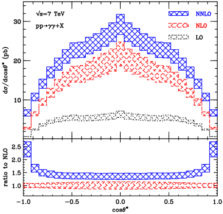
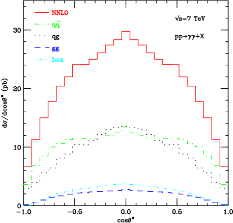
Figure 12: The differential cross section $d\sigma/d\cos\theta^{*}$. The results are analogous to those in Fig. 11.

The NNLO results for $d\sigma/d\cos\theta^{*}$ (and the corresponding results at LO and NLO) are presented in Fig. 12. The main features of the shape of $d\sigma/d\cos\theta^{*}$ are discussed in detail in Sects. 2.3.2 and 2.3.3. By direct inspection of the NLO (and LO) results in Fig. 4 and Fig. 12-left, we note that the shape of $d\sigma/d\cos\theta^{*}$ in Fig. 12-left is slightly different in the central region ($|\cos\theta^{*}|\raisebox{-2.58334pt}{\hbox to0.0pt{$\,\sim\,$\hss}}\raisebox{1.72218pt}{$\,<\,$}0.5$), since it tends to be more sharpened as $\cos\theta^{*}\rightarrow 0$. This shape distortion between the results in Fig. 4 and Fig. 12 is basically produced by the exclusion of the photon rapidity region $1.37<|y_{\gamma}|<1.52\,$ in the case of Fig. 12.

In the central region ($|\cos\theta^{*}|\raisebox{-2.58334pt}{\hbox to0.0pt{$\,\sim\,$\hss}}\raisebox{1.72218pt}{$\,<\,$}0.5$) we have $K^{NNLO}(\cos\theta^{*})\simeq 1.4\,$. This value of the NNLO $K$ factor and its scale dependence are remarkably similar to those of the corresponding $K$ factors for both the differential cross section $d\sigma/dM_{\gamma\gamma}$ in the high-mass region and the total cross section. In this $\cos\theta^{*}$ region the $q{\bar{q}}$ and $qg$ channels give comparable NNLO contribution to $d\sigma/d\cos\theta^{*}$ (the NNLO contribution of the $gg$ channel is small, at the level of about 10%), as shown in Fig. 12-right. All these features are perfectly consistent with the fact (as discussed in detail in Sect. 2.3.2; see, in particular, the second paragraph below Eq. (18)) that the central $\cos\theta^{*}$ region is kinematically strongly correlated (through the photon $p_{T}$ cuts) to the $M_{\gamma\gamma}$ region that gives the bulk of the total cross section.

At large values of $|\cos\theta^{*}|$ ($|\cos\theta^{*}|\raisebox{-2.58334pt}{\hbox to0.0pt{$\,\sim\,$\hss}}\raisebox{1.72218pt}{$\,>\,$}0.5$), the size of the NNLO corrections to $d\sigma/d\cos\theta^{*}$ increases by increasing $|\cos\theta^{*}|$ (see Fig. 12-left). In the second bin ($0.84<|\cos\theta^{*}|<0.92$) we have $K^{NNLO}(\cos\theta^{*})\simeq 1.7$, and in the first bin ($0.92<|\cos\theta^{*}|<1$) we have $K^{NNLO}(\cos\theta^{*})\simeq 2.4$ (the NNLO scale dependence also increases in the first bin). As discussed in Sect. 2.3.2, the large $|\cos\theta^{*}|$ region is kinematically more sensitive to high values of $M_{\gamma\gamma}$ (values of $M_{\gamma\gamma}$ higher than those that mostly contribute to the total cross section), and it is also relatively more sensitive to the angular distribution of the underlying partonic hard-scattering processes. In particular, this region can receive enhanced NNLO corrections from the $q{\bar{q}}$ and $qq$ initiated processes in Eqs. (32) and (33). The increasing value of $K^{NNLO}(\cos\theta^{*})$ at large $|\cos\theta^{*}|$ is consistent with our comments that accompany Eqs. (30)–(33) in Sect. 2.3.3 . As shown in Fig. 12-right, the relative NNLO contribution to $d\sigma/d\cos\theta^{*}$ of the $q{\bar{q}}$ channel increases in the region where $|\cos\theta^{*}|\raisebox{-2.58334pt}{\hbox to0.0pt{$\,\sim\,$\hss}}\raisebox{1.72218pt}{$\,>\,$}0.5$. This increasing behaviour of the $q{\bar{q}}$ channel is consistent with that observed at high values of $M_{\gamma\gamma}$ (see Fig. 11-right).

The NNLO (and NLO) results for the differential cross sections $d\sigma/d\Delta\Phi_{\gamma\gamma}$ and $d\sigma/dp_{T\gamma\gamma}$ are presented in Fig. 13. These differential cross sections have some similarities and some differences.

The similarities certainly regard the Sudakov sensitive region, namely the region that is close to the exclusive boundary of the phase space (either $\Delta\Phi_{\gamma\gamma}\sim\pi$ or $p_{T\gamma\gamma}\sim 0$). In this region the LO result (which is not shown in Fig. 13) is non-vanishing only in the most extreme bin (the bin that includes either $\Delta\Phi_{\gamma\gamma}=\pi$ or $p_{T\gamma\gamma}=0$). As already recalled in Sect. 2.3.3, fixed-order QCD computations of $d\sigma/dp_{T\gamma\gamma}$ at small values of $p_{T\gamma\gamma}$ are affected by large logarithmic contributions (powers of $\ln(M_{\gamma\gamma}/p_{T\gamma\gamma})\sim\ln(M^{LO}/p_{T\gamma\gamma})$) that invalidate the physical predictivity of the fixed-order result. Since $p_{T\gamma\gamma}\rightarrow 0$ implies $\Delta\Phi_{\gamma\gamma}\rightarrow\pi$, ensuing large logarithms ($\ln(\pi-\Delta\Phi_{\gamma\gamma})$) appears in the fixed-order computation of $d\sigma/d\Delta\Phi_{\gamma\gamma}$. These large logarithmic corrections produce a rapid change of the shape of the differential cross section order-by-order in QCD perturbation theory. Such a variation of shape is clearly visible in the results of Fig. 13-left for $\Delta\Phi_{\gamma\gamma}\raisebox{-2.58334pt}{\hbox to0.0pt{$\,\sim\,$\hss}}\raisebox{1.72218pt}{$\,>\,$}2.8$ and Fig. 13-right for $p_{T\gamma\gamma}\raisebox{-2.58334pt}{\hbox to0.0pt{$\,\sim\,$\hss}}\raisebox{1.72218pt}{$\,<\,$}15$ GeV (see, in particular, the shape of $K^{NNLO}$ in the lower subpanels of Fig. 13). As a consequence of this shape variation, the NLO and NNLO results tend to overlap (leading to $K^{NNLO}\sim 1$) in a tiny region. This overlap and the much reduced scale dependence of the NNLO result in this region should not be regarded as a signal of perturbative convergence: in contrast, they are just a consequence and an artifact of the order-by-order perturbative instability of the shape of the differential cross section (see Ref. [98] and, in particular, Sect. 3 therein for a completely related discussion in the context of $Z$ production). In the Sudakov sensitive region, reliable QCD predictions requires all-order resummation of the large logarithmic contributions [42, 43].

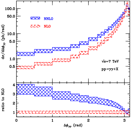
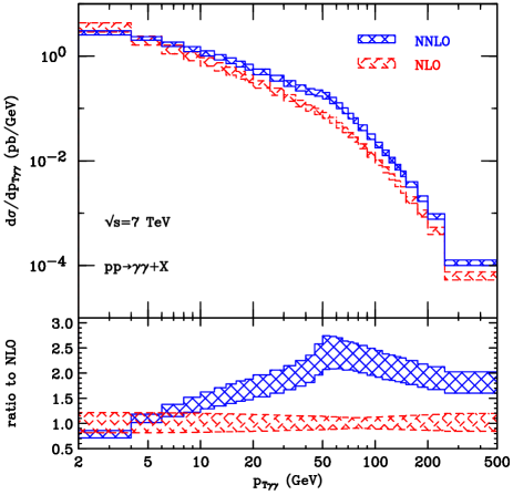
Figure 13: The differential cross sections $d\sigma/d\Delta\Phi_{\gamma\gamma}$ (left) and $d\sigma/dp_{T\gamma\gamma}$ (right). The NLO and NNLO results are analogous to those in Fig. 11.

The NNLO contribution of the various initial-state partonic channels to $d\sigma/dp_{T\gamma\gamma}$ in the region where $p_{T\gamma\gamma}<40$ GeV is presented in Fig. 14. Note that the partial contribution of the box $gg\rightarrow\gamma\gamma$ amplitude is non-vanishing only in the lowest-$p_{T\gamma\gamma}$ bin ($p_{T\gamma\gamma}<2$ GeV). In this first bin the $q{\bar{q}}$ and $gg$ channels give comparable and positive contributions to the NNLO differential cross section, while the contribution of the $qg$ channel is large and negative (it is outside the range of the vertical scale in Fig. 14). If $p_{T\gamma\gamma}>2$ GeV the $gg$ channel always gives a minor contribution: in particular, the contribution is negative in the entire $p_{T\gamma\gamma}$ region (excluding the lowest-$p_{T\gamma\gamma}$ bin) of Fig. 14, and it becomes positive at larger values of $p_{T\gamma\gamma}$. At very low values of $p_{T\gamma\gamma}$, the $q{\bar{q}}$ channel gives the largest NNLO contribution (this channel is responsible for the dominant logarithmic enhancement at small values of $p_{T\gamma\gamma}$). By increasing the value of $p_{T\gamma\gamma}$, the $qg$ channel tends to give the largest NNLO contribution because of its larger PDF luminosity. The contribution of the $qg$ channel remains the largest also in the region where $p_{T\gamma\gamma}>40$ GeV.

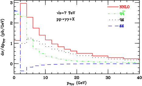
Figure 14: The NNLO cross section $d\sigma/dp_{T\gamma\gamma}$ at central scales in the low-$p_{T\gamma\gamma}$ region of Fig. 13-right. The NNLO result is decomposed in the contributions of different initial-state partonic channels: $q{\bar{q}}$ (green dot-dashed), $qg$ (black dotted) and $gg$ (blue dashed). The box $gg\rightarrow\gamma\gamma$ squared amplitude only contributes in the first (lowest-$p_{T\gamma\gamma}$) bin.

We do not explicitly report the decomposition of $d\sigma^{NNLO}/d\Delta\Phi_{\gamma\gamma}$ in initial-state partonic channels, since it is qualitatively similar to the decomposition in Fig. 13 through the correspondence (low $p_{T\gamma\gamma})\leftrightarrow$ (large $\Delta\Phi_{\gamma\gamma}$) and (large $p_{T\gamma\gamma})\leftrightarrow$ (small $\Delta\Phi_{\gamma\gamma}$). In particular, the $q{\bar{q}}$ channel gives the largest NNLO contribution at $\Delta\Phi_{\gamma\gamma}\raisebox{-2.58334pt}{\hbox to0.0pt{$\,\sim\,$\hss}}\raisebox{1.72218pt}{$\,>\,$}3$, whereas the $qg$ channel gives the largest contribution at moderate and small values of $\Delta\Phi_{\gamma\gamma}$. The contribution of the $gg$ channel is always small and, in particular, it is negative at $\Delta\Phi_{\gamma\gamma}\raisebox{-2.58334pt}{\hbox to0.0pt{$\,\sim\,$\hss}}\raisebox{1.72218pt}{$\,>\,$}2.7\,$.

Outside the Sudakov sensitive region the LO result vanishes and, therefore, the NNLO (NLO) results in Fig.13 are ‘effective’ NLO (LO) QCD predictions. We comment on the results for $d\sigma/d\Delta\Phi_{\gamma\gamma}$ and $d\sigma/dp_{T\gamma\gamma}$ in turn.

In the region from moderate to small values of $\Delta\Phi_{\gamma\gamma}$ (Fig. 13-left) the NNLO corrections monotonically increase by decreasing $\Delta\Phi_{\gamma\gamma}$. We have $K^{NNLO}(\Delta\Phi_{\gamma\gamma})\sim 2$ at $\Delta\Phi_{\gamma\gamma}\sim 2.5$, and $K^{NNLO}(\Delta\Phi_{\gamma\gamma})\simeq 3.4$ in the lowest-$\Delta\Phi_{\gamma\gamma}$ bin ($0<\Delta\Phi_{\gamma\gamma}<0.5$). The large size of the NNLO corrections at small $\Delta\Phi_{\gamma\gamma}$ was pointed out in Ref. [99]. The scale dependence of the NNLO result throughout this region is at the level of about $\pm 15$%, and it is basically unchanged with respect to the scale dependence of the NLO result.

In the region from moderate to large values of $p_{T\gamma\gamma}$ the size of the NNLO corrections does not have a monotonic dependence on $p_{T\gamma\gamma}$ (Fig. 13-right). We have $K^{NNLO}(p_{T\gamma\gamma})\sim 1.7$ at $p_{T\gamma\gamma}\sim 20$ GeV and $K^{NNLO}(p_{T\gamma\gamma})\simeq 1.8$ in the highest-$p_{T\gamma\gamma}$ bin ($250~{}{\rm GeV}<p_{T\gamma\gamma}<500$ GeV); at these values of $p_{T\gamma\gamma}$ the NNLO scale dependence is at the level of about $\pm 12$% (the corresponding NLO scale dependence is about $\pm 18$%). In the intermediate $p_{T\gamma\gamma}$ region, the size of the NNLO corrections has a maximal value at $p_{T\gamma\gamma}\sim 50$ GeV. In the bin with $50~{}{\rm GeV}<p_{T\gamma\gamma}<55$ GeV we have $K^{NNLO}(p_{T\gamma\gamma})\simeq 2.4$ with a scale dependence of about $\pm 15$% (it is basically the same scale dependence as at NLO, since in the region where $50~{}{\rm GeV}\raisebox{-2.58334pt}{\hbox to0.0pt{$\,\sim\,$\hss}}\raisebox{1.72218pt}{$\,<\,$}p_{T\gamma\gamma}\raisebox{-2.58334pt}{\hbox to0.0pt{$\,\sim\,$\hss}}\raisebox{1.72218pt}{$\,<\,$}100$ GeV the NLO scale dependence tends to be minimal).

The NNLO results for $d\sigma/d\Delta\Phi_{\gamma\gamma}$ and $d\sigma/dp_{T\gamma\gamma}$ deserve some overall comments.

We first note that the size of the NNLO corrections to $d\sigma/d\Delta\Phi_{\gamma\gamma}$ and $d\sigma/dp_{T\gamma\gamma}$ is typically larger than that of the NNLO corrections to the total cross section, to $d\sigma/dM_{\gamma\gamma}$ at high masses and to $d\sigma/d\cos\theta^{*}$. This feature is consistent with the fact that we are dealing with ‘effective’ NLO (rather than NNLO) QCD predictions in the case of the $\Delta\Phi_{\gamma\gamma}$ and $p_{T\gamma\gamma}$ differential cross sections.

Then, we also observe a hierarchy of the size of the NNLO corrections for various differential cross sections that are computed at ‘effective’ NLO: $K^{NNLO}(M_{\gamma\gamma})$ at low $M_{\gamma\gamma}$ is larger than $K^{NNLO}(\Delta\Phi_{\gamma\gamma})$ at small $\Delta\Phi_{\gamma\gamma}$, which is in turn larger than $K^{NNLO}(p_{T\gamma\gamma})$ at moderate and large values of $p_{T\gamma\gamma}$. This hierarchy is in agreement with the expectations of our discussion in Sect. 2.3.3. In particular, it is qualitatively consistent with the effect of the NNLO processes in Eqs. (28) and (29): they are dynamically enhanced at small values of $M_{\gamma\gamma}$ (see the accompanying comments to Eqs. (28) and (29)) and, because of kinematics, they are still enhanced but with a decreasing relevance at small $\Delta\Phi_{\gamma\gamma}$ and, in turn, at large $p_{T\gamma\gamma}$.

Finally, we note that the values of $K^{NNLO}$ for $d\sigma/d\Delta\Phi_{\gamma\gamma}$ and $d\sigma/dp_{T\gamma\gamma}$ within smooth isolation are larger than the corresponding differences between standard and smooth isolation results at NLO (see Sect. 2.3.3). This fact and the discussion throughout the paper is a strong indication of the presence of sizeable NNLO radiative corrections to diphoton production also within the standard cone isolation criterion.

We present some additional comments on $d\sigma/dp_{T\gamma\gamma}$ in the region of relatively-large values of $p_{T\gamma\gamma}$. As we have noticed in Sect. 2.3.3, the NLO standard isolation results in Fig. 8-right have a shoulder-type behaviour at $p_{T\gamma\gamma}\sim 50$ GeV. The $p_{T\gamma\gamma}$ shoulder is also visible in the NNLO smooth isolation results of Fig. 13-right (see also Figs. 15-left and 18-right, which have a linear scale in $p_{T\gamma\gamma}$), although it is less pronounced since the results refer to $E_{T\,{\rm max}}=4$ GeV, which is smaller than the value $E_{T\,{\rm max}}=10$ GeV of Fig. 8-right. As previously recalled, in the context of standard isolation the $p_{T\gamma\gamma}$ shoulder was discussed in Ref. [95]. Here we present related comments in the context of the smooth isolation criterion.

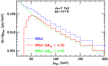
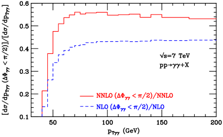
Figure 15: Left panel: the NNLO cross section $d\sigma/dp_{T\gamma\gamma}$ (blue dashed) in Fig. 13-right and its partition into the contributions from the two complementary regions where $\Delta\Phi_{\gamma\gamma}>\pi/2$ (green dotted) and $\Delta\Phi_{\gamma\gamma}<\pi/2$ (red solid). Right panel: the fractional contribution to $d\sigma/dp_{T\gamma\gamma}$ from the region where $\Delta\Phi_{\gamma\gamma}<\pi/2$ at NLO (blue dashed) and NNLO (red solid).

We follow Ref. [95] and we consider the partition of $d\sigma/dp_{T\gamma\gamma}$ in the contributions of the two complementary kinematical regions with relatively-large ($\Delta\Phi_{\gamma\gamma}>\pi/2$) and relatively-small ($\Delta\Phi_{\gamma\gamma}<\pi/2$) values of $\Delta\Phi_{\gamma\gamma}$. These contributions are denoted by $d\sigma^{(l)}/dp_{T\gamma\gamma}$ (if $\Delta\Phi_{\gamma\gamma}>\pi/2$) and $d\sigma^{(s)}/dp_{T\gamma\gamma}$ (if $\Delta\Phi_{\gamma\gamma}<\pi/2$) in the following text. The complete NNLO result for $d\sigma/dp_{T\gamma\gamma}$ and the corresponding NNLO results from the two complementary regions of $\Delta\Phi_{\gamma\gamma}$ are presented in Fig. 15-left at values of $p_{T\gamma\gamma}$ around the shoulder. The component $d\sigma^{(l)}/dp_{T\gamma\gamma}$ has an approximately-constant slope at $p_{T\gamma\gamma}\raisebox{-2.58334pt}{\hbox to0.0pt{$\,\sim\,$\hss}}\raisebox{1.72218pt}{$\,>\,$}30$ GeV, whereas the total contribution tends to flatten out at $p_{T\gamma\gamma}\sim 50$ GeV and it remains systematically higher than $d\sigma^{(l)}/dp_{T\gamma\gamma}$ at larger values of $p_{T\gamma\gamma}$. These differences are obviously due to the component $d\sigma^{(s)}/dp_{T\gamma\gamma}$, which exactly vanishes at $p_{T\gamma\gamma}\raisebox{-2.58334pt}{\hbox to0.0pt{$\,\sim\,$\hss}}\raisebox{1.72218pt}{$\,<\,$}34$ GeV and has a maximum value at $p_{T\gamma\gamma}\sim 50$ GeV.

To comment on the behaviour of the results in Fig. 15-left we consider the effect of the kinematical constraint in Eq. (24) (see also its accompanying comments), which is a consequence of the photon $p_{T}$ cuts. The component $d\sigma^{(l)}/dp_{T\gamma\gamma}$ is insensitive to the constraint. Moving from large to smaller values of $p_{T\gamma\gamma}$, the size of this component increases since the production of photons with smaller transverse momenta is kinematically (because of energy conservation) and also dynamically favoured. At $\Delta\Phi_{\gamma\gamma}\sim 0$, the constraint in Eq. (24) leads to $p_{T\gamma\gamma}\raisebox{-2.58334pt}{\hbox to0.0pt{$\,\sim\,$\hss}}\raisebox{1.72218pt}{$\,>\,$}47$ GeV (see Eq. (25)). Therefore, provided $p_{T\gamma\gamma}\raisebox{-2.58334pt}{\hbox to0.0pt{$\,\sim\,$\hss}}\raisebox{1.72218pt}{$\,>\,$}47$ GeV, the entire kinematical region of $\Delta\Phi_{\gamma\gamma}$ is kinematically allowed and $d\sigma^{(s)}/dp_{T\gamma\gamma}$ is also insensitive to the constraint. It follows that at large values of $p_{T\gamma\gamma}$ both components (and their total contribution) show a similar increasing behaviour as $p_{T\gamma\gamma}$ decreases. If $p_{T\gamma\gamma}\raisebox{-2.58334pt}{\hbox to0.0pt{$\,\sim\,$\hss}}\raisebox{1.72218pt}{$\,<\,$}47$ GeV the constraint in Eq. (24) is instead effective on $d\sigma^{(s)}/dp_{T\gamma\gamma}$ and, consequently, on the total contribution to $d\sigma/dp_{T\gamma\gamma}$. Going from $p_{T\gamma\gamma}\simeq 47$ GeV to smaller values of $p_{T\gamma\gamma}$, the kinematical constraint forbids the region of small values of $\Delta\Phi_{\gamma\gamma}$: consequently, the increasing behaviour of $d\sigma/dp_{T\gamma\gamma}$ flattens out since $d\sigma^{(s)}/dp_{T\gamma\gamma}$ is increasingly suppressed. In particular, Eq. (24) implies the restriction $p_{T\gamma\gamma}\raisebox{-2.58334pt}{\hbox to0.0pt{$\,\sim\,$\hss}}\raisebox{1.72218pt}{$\,>\,$}34$ GeV if $\Delta\Phi_{\gamma\gamma}<\pi/2$ and, therefore, $d\sigma^{(s)}/dp_{T\gamma\gamma}$ has a kinematical threshold at $p_{T\gamma\gamma}\simeq 34$ GeV.

From our discussion on the results in Fig. 15-left, it follows that the onset of the shoulder at $p_{T\gamma\gamma}\sim 50$ GeV is kinematically driven (by the presence of the photon $p_{T}$ cuts). However, it also has a dynamical component, since the NNLO corrections enhance this effect (see the size of $K^{NNLO}(p_{T\gamma\gamma})$ at $p_{T\gamma\gamma}\raisebox{-2.58334pt}{\hbox to0.0pt{$\,\sim\,$\hss}}\raisebox{1.72218pt}{$\,>\,$}50$ GeV in Fig. 13-right).

To remark the NNLO enhancement we compute the ratio between $d\sigma^{(s)}/dp_{T\gamma\gamma}$ and $d\sigma/dp_{T\gamma\gamma}$, namely, the fractional contribution to $d\sigma/dp_{T\gamma\gamma}$ from the region of relatively-small values of $\Delta\Phi_{\gamma\gamma}$. In Fig. 15-right we present the results for this ratio at both NNLO and NLO (the shape of $d\sigma^{(s)}/dp_{T\gamma\gamma}$ at NLO is qualitatively similar to that of the corresponding NNLO result in Fig. 15-left). At both perturbative orders this ratio is sizeable and approximately independent of $p_{T\gamma\gamma}$ in the region just above $p_{T\gamma\gamma}\sim 50$ GeV: the ratio is about 0.42 at NLO and 0.54 at NNLO. Therefore, the region where $\Delta\Phi_{\gamma\gamma}<\pi/2$ contributes to roughly half of the complete differential cross section $d\sigma/dp_{T\gamma\gamma}$ at $p_{T\gamma\gamma}\raisebox{-2.58334pt}{\hbox to0.0pt{$\,\sim\,$\hss}}\raisebox{1.72218pt}{$\,>\,$}50$ GeV, and this fact has a kinematical origin. The increase of about 30% of the ratio from the NLO to the NNLO result has instead a dynamical origin (incidentally, this increase implies that the NNLO $K$ factor for $d\sigma^{(s)}/dp_{T\gamma\gamma}$ is larger than that for $d\sigma/dp_{T\gamma\gamma}$ in Fig.13-right). It is due to the NNLO processes in Eqs. (28) and (29) that are dynamically enhanced at small values of $M_{\gamma\gamma}$ and, consequently (see Eq. (23) and accompanying comments), partly enhanced also at very small values of $\Delta\Phi_{\gamma\gamma}$. There are dynamical similarities between these processes and the NLO fragmentation processes in Eqs. (26) and (27), which, according to Ref. [95], originate the $p_{T\gamma\gamma}$ shoulder in the NLO standard isolation results. Therefore, our discussion on the $p_{T\gamma\gamma}$ shoulder in the NNLO smooth isolation results is consistent with the observations in Ref. [95].

The partition of the phase space into the two regions with $\Delta\Phi_{\gamma\gamma}>\pi/2$ and $\Delta\Phi_{\gamma\gamma}<\pi/2$ was applied by the D0 Collaboration [6] to diphoton production data in proton–antiproton collisions at the Tevatron. The results in Ref. [6] show that the inclusion of the NNLO corrections considerably improves the description of the data in both phase space regions.

3.3 Dependence on isolation parameters

We add some illustrative results and comments on differential cross sections at NNLO and their dependence on isolation parameters.

We use $d\sigma/d\cos\theta^{*}$ and $d\sigma/d\Delta\Phi_{\gamma\gamma}$ as representative cross sections of typical features of the NNLO results. We consider the corresponding reference NNLO results of this section (Figs. 12 and 13), which are obtained with $E_{T\,{\rm max}}=4$ GeV and the power $n=1$ in the isolation function $\chi(r;R)$, and we perform variations of the isolation parameters $E_{T\,{\rm max}}$ and $n$. Specifically, we use either $n=0.5$ or $n=2$ by keeping $E_{T\,{\rm max}}=4$ GeV fixed, and we use $n=1$ by increasing $E_{T\,{\rm max}}$ to the value $E_{T\,{\rm max}}=10$ GeV. The ensuing NNLO results are presented in Fig. 16. In the lower subpanels of Fig. 16 we present the ratio of the results with different isolation parameters with respect to the reference NNLO result ($n=1$, $E_{T\,{\rm max}}=4$ GeV). All these results are obtained with central values of the scales ($\mu_{R}=\mu_{F}=\mu_{0}=M_{T\gamma\gamma}$). The scale dependence of the reference NNLO result is also reported in Fig. 16 for comparison with isolation parameters effects.

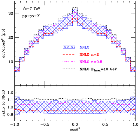
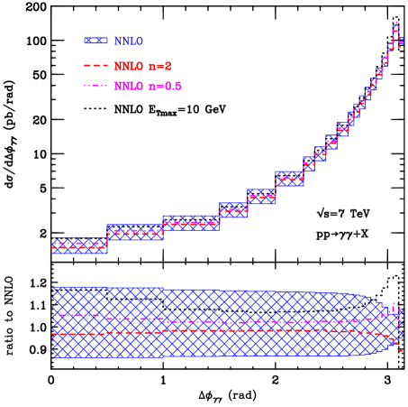
Figure 16: Isolation parameter dependence of $d\sigma/d\cos\theta^{*}$ (left) and $d\sigma/d\Delta\Phi_{\gamma\gamma}$ (right) at NNLO. The reference results (including their scale dependence) with $n=1$ and $E_{T\,{\rm max}}=4$ GeV of Figs.12 and 13 are compared to corresponding results that are obtained by varying either $n$ ($n=2$ and $n=0.5$) or $E_{T\,{\rm max}}$ ($E_{T\,{\rm max}}=10$ GeV). Cross sections ratios with respect to the reference result are shown in the lower subpanels.

We comment on the results in Fig. 16 by excluding those in the region where $\Delta\Phi_{\gamma\gamma}\raisebox{-2.58334pt}{\hbox to0.0pt{$\,\sim\,$\hss}}\raisebox{1.72218pt}{$\,>\,$}2.8$ (comments on this region are postponed). As a main overall comment we observe that the NNLO results have a mild dependence on the isolation parameters. Indeed, the effects of the variations of the isolation parameters are not larger than the scale dependence at fixed isolation parameters. Moreover, the qualitative dependence on both $E_{T\,{\rm max}}$ and $n$ is in agreement with physical expectation (see Eqs. (6) and (8)) throughout the entire kinematical regions of $\cos\theta^{*}$ and $\Delta\Phi_{\gamma\gamma}$: the value of the differential cross sections decreases by requiring the photons to be more isolated. We also recall (see Sect. 2.3.3) that in the region where $\Delta\Phi_{\gamma\gamma}\raisebox{-2.58334pt}{\hbox to0.0pt{$\,\sim\,$\hss}}\raisebox{1.72218pt}{$\,<\,$}\pi-R\simeq 2.7$ the NLO cross section $d\sigma/d\Delta\Phi_{\gamma\gamma}$ (within smooth isolation) does not depend on the isolation parameters. Therefore, the $E_{T\,{\rm max}}$ and $n$ dependence observed in the NNLO results for $d\sigma/d\cos\theta^{*}$ ($d\sigma/d\Delta\Phi_{\gamma\gamma}$) is ‘effectively’ an NLO (an LO) QCD effect.

We note that the $n$ dependence (at fixed $E_{T\,{\rm max}}=4$ GeV) is practically the same throughout the entire kinematical region of either $\cos\theta^{*}$ or $\Delta\Phi_{\gamma\gamma}$, so that it does not produce any shape variations. The overall size of the $n$ dependence of the differential cross sections is basically equal to that of the NNLO total cross section (see Sect. 3.1).

The $E_{T\,{\rm max}}$ dependence in Fig. 16 is substantially larger than the $n$ dependence, because $E_{T\,{\rm max}}=10$ GeV is sizeably different from $E_{T\,{\rm max}}=4$ GeV. Nonetheless, also the $E_{T\,{\rm max}}$ dependence at NNLO is quite moderate (as already noticed in Sect. 2.3.1 for the case of the NLO total cross section). In the case of $d\sigma^{NNLO}/d\cos\theta^{*}$, the variation of $E_{T\,{\rm max}}$ does not produce any significant shape variation: the differential cross section uniformly increases by approximately 10% in going from $E_{T\,{\rm max}}=4$ GeV to $E_{T\,{\rm max}}=10$ GeV. Consequently, an equal increase applies to the NNLO total cross section. We note that the size of the $E_{T\,{\rm max}}$ dependence is slightly larger at NNLO than at NLO (see Sect. 2.3.1); an analogous increased sensitivity to the value of $n$ (at fixed $E_{T\,{\rm max}}$) has been already noticed in Sect. 3.1 . In the case of $d\sigma^{NNLO}/d\Delta\Phi_{\gamma\gamma}$, the variation of $E_{T\,{\rm max}}$ also produces a visible shape dependence. In going from $E_{T\,{\rm max}}=4$ GeV to $E_{T\,{\rm max}}=10$ GeV, $d\sigma^{NNLO}/d\Delta\Phi_{\gamma\gamma}$ increases by approximately 8% at $\Delta\Phi_{\gamma\gamma}\sim 2$, and by approximately 16% at $\Delta\Phi_{\gamma\gamma}\sim 0.5\,$. This shape dependent effect is consistent with our previous discussions in Sect. 3.2 and in Sect. 2.3.3. At small values of $\Delta\Phi_{\gamma\gamma}$ the NNLO cross section $d\sigma^{NNLO}/d\Delta\Phi_{\gamma\gamma}$ receives substantial contribution from configurations in which the photons are accompanied by partonic (hadronic) transverse energy inside the isolation cones (see Eqs. (28) and (29)): by increasing $E_{T\,{\rm max}}$ these configurations are less suppressed by the isolation requirement and the cross section increases (a qualitatively similar $E_{T\,{\rm max}}$ dependence at small $\Delta\Phi_{\gamma\gamma}$ is observed in the NLO standard isolation results of Fig. 7).

On the basis of our discussion about the results in Fig. 16 and of our previous discussions about similarities between various NNLO differential cross sections, we can argue about the $E_{T\,{\rm max}}$ dependence of $d\sigma/dM_{\gamma\gamma}$ and $d\sigma/dp_{T\gamma\gamma}$ at NNLO. In the high-$M_{\gamma\gamma}$ region the $E_{T\,{\rm max}}$ dependence of $d\sigma/dM_{\gamma\gamma}$ is similar to that of $d\sigma/d\cos\theta^{*}$. The $E_{T\,{\rm max}}$ sensitivity of $d\sigma/dM_{\gamma\gamma}$ at small values of $M_{\gamma\gamma}$ is partly enhanced with respect to that of $d\sigma/d\Delta\Phi_{\gamma\gamma}$ at small $\Delta\Phi_{\gamma\gamma}$. The $E_{T\,{\rm max}}$ sensitivity of $d\sigma/dp_{T\gamma\gamma}$ at moderate and large values of $p_{T\gamma\gamma}$ is partly reduced with respect to that of $d\sigma/d\Delta\Phi_{\gamma\gamma}$ at small $\Delta\Phi_{\gamma\gamma}$.

We come to comment about the results in the large-$\Delta\Phi_{\gamma\gamma}$ region ($\Delta\Phi_{\gamma\gamma}\raisebox{-2.58334pt}{\hbox to0.0pt{$\,\sim\,$\hss}}\raisebox{1.72218pt}{$\,>\,$}2.8$) of Fig. 16. This is definitely part of the Sudakov sensitive region. We point out that here the dependence on the isolation parameters (both $E_{T\,{\rm max}}$ and $n$) is amplified with respect to the rest of the kinematical regions. We are dealing with diphoton production close to the exclusive boundary of the phase space, where the photon pair is accompanied by radiation of little transverse energy, also outside the photon isolation cones. In such a configuration the effects of variations of the isolation requirements are relatively enhanced at fixed order: therefore, an enhanced sensitivity to isolation parameters can be expected in the results of Fig. 16-right. As recalled in Sect. 3.2, the NNLO result (and, consequently, the ensuing isolation parameter dependence) is not physically reliable in this Sudakov sensitive region. Nonetheless, the observed isolation parameter dependence at NNLO indicates that photon isolation effects have to be carefully considered (and examined) in the context of refined resummed calculations in the Sudakov sensitive region.

3.4 Comparison of NNLO results and data

In Ref. [4] the ATLAS data on diphoton production at the centre–of–mass energy ${\sqrt{s}}=7$ TeV were compared with the NNLO QCD results. As stated in the conclusion of Ref. [4], the NNLO results are able to match the data very closely within the uncertainties, except in limited regions. In the following we present some comments on the comparison between NNLO results and data.

As a preliminary comment, we note that the NNLO results in Ref. [4] and those in this paper are not exactly equal. The differences have various origins. Part of the differences are due to the setup of the NNLO calculations. The results of the NNLO calculation presented in Ref. [4] use the PDFs of the MSTW2008 set, the central scale $\mu_{0}=M_{\gamma\gamma}$ and the scale dependence that is obtained by considering the scale configurations with $\mu_{R}=\mu_{F}=M_{\gamma\gamma}/2$ and with $\mu_{R}=\mu_{F}=2M_{\gamma\gamma}$. Here we use different PDFs, a different central scale and independent scale variations of $\mu_{R}$ and $\mu_{F}$. The other differences are due to the fact that the NNLO results of Ref. [4] were obtained by using the first version of the numerical program 2$\gamma$NNLO, which had an implementation error that was subsequently corrected [35]. All these effects produce differences between the NNLO results used in Ref. [4] and those reported here. Nonetheless the differences are relatively small (in particular, they are smaller than the scale dependence at NNLO) and they do not have a major effect on the comparison between NNLO results and data.

The ATLAS Collaboration performs a quantitative estimate of underlying event, pile-up and hadronization effects. These effects, which are not included in fixed-order QCD calculations, are taken into account [4] by applying a correction factor to the fixed-order QCD results. The typical size of the correction factor is around 0.95 [4]. The bin-by-bin correction factors for various differential cross sections are available in the database of the Durham HepData Project [100]. We apply these bin-by-bin correction factors to our NNLO calculations (for simplicity, we simply rescale the NNLO central values by the bin-by-bin corrections, without including the uncertainties of the correction factors themselves), and we present the ensuing results in Figs. 17 and 18.

A technical comment about Fig. 17 regards the differential cross section $d\sigma/d\cos\theta^{*}$. Since the two photons of the diphoton pair are identical particles, $d\sigma/d\cos\theta^{*}$ is symmetric with respect to $\cos\theta^{*}\leftrightarrow-\cos\theta^{*}$. In our QCD results throughout this paper we have always computed the differential cross section with respect to $|\cos\theta^{*}|$ and then the results are presented in symmetrized form. In the ATLAS data, $\cos\theta^{*}$ refers to the cosine of the polar angle $\theta^{*}$ of the harder photon (the photon with momentum $p_{T\gamma}^{hard}$) and, consequently (because of experimental effects in the measurement, including statistical fluctuations), $d\sigma/d\cos\theta^{*}$ is not exactly symmetric under $\cos\theta^{*}\leftrightarrow-\cos\theta^{*}$ (although it is symmetric within the experimental errors). The NNLO result in Fig. 17-right is not exactly symmetric because of the non-symmetric correction factors that have been applied.

A main general comment about the comparison between data and NNLO results regards the photon isolation criteria. The ATLAS data use standard isolation (though the experimental details of the actual isolation procedure are quite involved and differ from a plain implementation of standard isolation), whereas the NNLO results use smooth isolation with the same values of the isolation parameters $R$ and $E_{T\,{\rm max}}$. In our opinion the comparison is meaningful despite the differences between the isolation criteria. This follows from several observations that we list. Owing to the physical constraint in Eq. (5), NNLO results for smooth isolation give a lower bound on the NNLO results for standard isolation. Smooth and standard isolation results are quantitatively quite similar starting from computations at ‘effective’ NLO accuracy (see Sects. 2.3.1 and 2.3.3), and such similarity is expected to remain valid at NNLO (see, e.g., the mild dependence on isolation parameters that we noticed in Sect. 3.3). Calculations within both isolation criteria are affected by sizeable higher-order corrections, and at ‘effective’ NLO accuracy these corrections tend to be larger than the differences between the NLO results for smooth and standard isolation (see Sects. 2.3.1–2.3.3). Therefore, neglecting NNLO effects can have more impact than using different isolation criteria. Reference [4] compares the ATLAS data to both NNLO results for smooth isolation and lower-order results for standard isolation: the differences between these fixed-order results confirm that NNLO corrections are sizeable and relevant. Obviously all these observations about smooth and standard isolation results are valid within the corresponding perturbative uncertainties.

We present more specific comments about total and differential cross sections.

The experimental value of the total cross section is [4] $\sigma_{ATLAS}=44.0~{}^{+3.2}_{-4.2}$ pb. We compute the corresponding NNLO result from the bin-by-bin corrected differential cross section $d\sigma/d\cos\theta^{*}$ (Fig. 17-right), and we obtain $\sigma_{ATLAS}^{NNLO}=37.2~{}^{+3.2}_{-3.3}\rm{(scale)}$ pb. The measured value and the NNLO result are consistent within the corresponding experimental and scale dependence uncertainties. Moreover, as remarked in Sect. 3.1, the NNLO scale dependence cannot be regarded as a consistent estimate of the perturbative uncertainty due to uncalculated higher-order terms. The ‘true’ perturbative uncertainty of $\sigma^{NNLO}$ is larger than the scale dependent effect that we have computed. A better uncertainty estimate can be obtained, for instance, by considering enlarged scale variations, such that the ensuing NNLO and NLO results have some degree of overlap. An alternative, similar and simpler procedure consists in comparing the NNLO and NLO results at central values of the scales (incidentally, we have checked that NLO results for smooth and standard isolation are quantitatively very similar) and using half of the difference between them to assign the perturbative uncertainty of the NNLO result. This procedure leads (see Table 2) to an NNLO uncertainty of about $\pm 14$%, which amounts to almost double the scale uncertainty of the NNLO result for the total cross section.

The ATLAS data [4] on differential cross sections are reported in Figs. 17 and 18 together with the corresponding NNLO results. In the lower subpanels of these figures we present the ratio between the data and the NNLO results at central scales, and the scale dependence of the NNLO results.

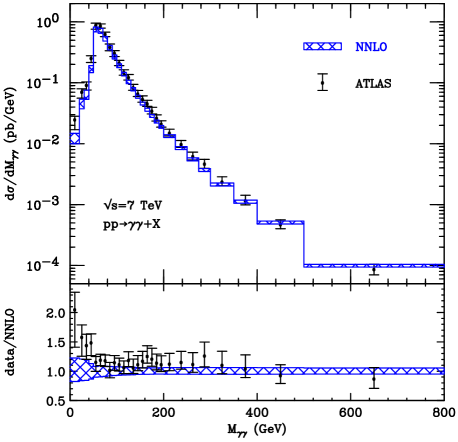
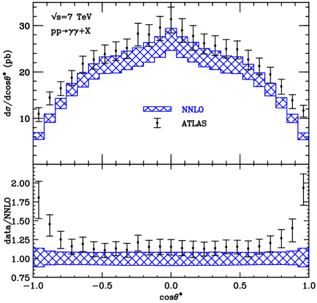
Figure 17: Comparison between ATLAS data at ${\sqrt{s}}=7$ TeV [4] and NNLO results (including their scale dependence) for $d\sigma/dM_{\gamma\gamma}$ (left) and $d\sigma/d\cos\theta^{*}$ (right). The NNLO results are corrected for hadronization and underlying event effects (see text).

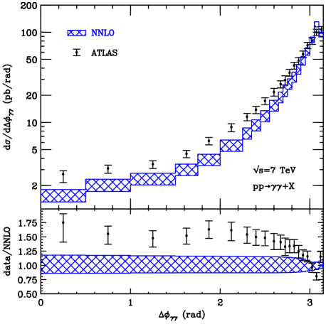
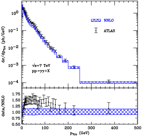
Figure 18: Comparison between ATLAS data at ${\sqrt{s}}=7$ TeV [4] and NNLO results (including their scale dependence) for $d\sigma/d\Delta\Phi_{\gamma\gamma}$ (left) and $d\sigma/dp_{T\gamma\gamma}$ (right). The NNLO results are corrected for hadronization and underlying event effects (see text).

At large values of $\Delta\Phi_{\gamma\gamma}$ (e.g., $\Delta\Phi_{\gamma\gamma}\raisebox{-2.58334pt}{\hbox to0.0pt{$\,\sim\,$\hss}}\raisebox{1.72218pt}{$\,>\,$}2.8$) and small values of $p_{T\gamma\gamma}$ (e.g., $p_{T\gamma\gamma}\raisebox{-2.58334pt}{\hbox to0.0pt{$\,\sim\,$\hss}}\raisebox{1.72218pt}{$\,<\,$}20$ GeV) the shape of the data (Fig. 18) is definitely different from that of the NNLO results. This is expected since, as discussed in Sect. 3.2, the shape of the NNLO results is not physically reliable in these Sudakov sensitive regions. All-order resummed calculations [42, 43, 8] have to be used here. All-order resummation effects are implemented also in parton shower event generators, which can lead to a consistent description of the data [4, 8].

The NNLO results in Fig. 18 (outside the Sudakov sensitive regions) and those in the low-mass region ($M_{\gamma\gamma}<50$ GeV) of Fig. 17-left are perturbative results at ‘effective’ NLO accuracy, while those in the high-mass region and in the entire region of $\cos\theta^{*}$ (Fig. 17) are results at ‘effective’ NNLO accuracy. In ‘effective’ NNLO regions there is a good agreement between data and NNLO results within the corresponding experimental and scale uncertainties. In ‘effective’ NLO regions the data tend to be systematically higher than the NNLO results at central values of the scales. Note that the shape of the differences between data and NNLO results tends to qualitatively follow the shape of the NNLO $K$ factors (see the lower subpanels in Figs. 17 and 18 and those in Figs. 11, 12 and 13). This feature is consistent with our previous remarks on the fact (see the differences between NLO and NNLO results in Figs. 11, 12 and 13) that the computed scale dependence at NNLO does underestimate the true perturbative uncertainties of the NNLO results. If we proceed to assign a perturbative uncertainty on the basis of the differences between NNLO and NLO results for differential cross sections (analogously to the procedure that we have previously mentioned for the total cross section in this subsection), the NNLO uncertainty is almost doubled with respect to the NNLO scale dependence in most of the regions of Figs. 17 and 18 and it is further increased in limited extreme regions (such as at very small values of $M_{\gamma\gamma}$, at very large values of $|\cos\theta^{*}|$ and at very low values of $\Delta\Phi_{\gamma\gamma}$). Such an NNLO uncertainty makes the ATLAS data consistent with the NNLO results in both ‘effective’ NNLO and ‘effective’ NLO regions.

The tendency of the data to be systematically higher than the NNLO results at central values of the scales is not inconsistent with the expectation (see Eq. (5)) that the NNLO results with smooth isolation should be a lower bound on the corresponding results for standard isolation. One can try to reduce the differences between the smooth and standard isolation criteria by decreasing the isolation effects within smooth isolation. This can be done by using different smooth isolation parameters such as, for instance, a smaller value of the power $n$ of the isolation function $\chi(r;R)$ or a larger value of $E_{T\,{\rm max}}$. As shown by the results in Sect. 3.3, such a procedure can reduce the systematic differences between ATLAS data and NNLO smooth isolation results. Nonetheless, this ‘tuning’ procedure does not affect the overall features of the comparison between data and NNLO results, because of the relatively-small dependence on the isolation parameters (see Sect. 3.3) and of the substantial NNLO theoretical uncertainties that we have previously discussed.

In this subsection we have considered the ATLAS diphoton data at ${\sqrt{s}}=7$ TeV and we have presented comments on the main features of the data/NNLO comparison. The same features and comments are equally valid for other LHC diphoton measurements [7, 8] and related data/theory comparisons [7, 8, 37]. In particular, the inclusion of the NNLO radiative corrections greatly improves the description of the data [4, 7, 8] with respect to lower-order results. The effect of the NNLO corrections is from moderate to sizeable in different kinematical regions. This leads to a good or consistent (depending on kinematical regions) agreement with the data by taking into account the perturbative uncertainty of the NNLO results.

3.5 Asymmetric and symmetric photon $p_{T}$ cuts

Throughout the paper we have remarked that the presence of the photon $p_{T}$ cuts ($p_{T\gamma}^{hard}\geq p_{H},\;p_{T\gamma}^{soft}\geq p_{S}$) has relevant effects on various features of diphoton production observables. All the numerical results presented so far (with the exception of those in Fig. 6) use the values $p_{H}=25$ GeV and $p_{S}=22$ GeV. In this subsection we present some results and related comments on effects that are due to variations of $p_{H}$ and $p_{S}$. In particular, we consider symmetric $p_{T}$ cut configurations ($p_{H}=p_{S}$) in addition to asymmetric configurations ($p_{H}>p_{S}$).

We consider the reference kinematical configuration (and theoretical setup) used throughout this section, but we vary the photon $p_{T}$ cuts $p_{H}$ and $p_{S}$. All the numerical results presented in this subsection refer to the central value of the scales ($\mu_{R}=\mu_{F}=\mu_{0}={\sqrt{M_{\gamma\gamma}^{2}+p_{T\gamma\gamma}^{2}}}\,\;$).

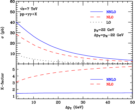
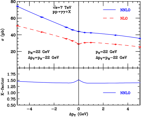
Figure 19: Dependence on the photon $p_{T}$ cuts $p_{H}$ and $p_{S}$ ($p_{T\gamma}^{hard}\geq p_{H},\;p_{T\gamma}^{soft}\geq p_{S}$) of the total cross section for diphoton production (the other kinematical cuts are the same as in Table 2). The NLO (red dashed) and NNLO (blue solid) results are separately presented in the regions of asymmetric (left panel) and nearly-symmetric (right panel) $p_{T}$ cuts. The LO result (black dotted) is presented only in the case of asymmetric $p_{T}$ cuts (left panel). The lower subpanels present the corresponding NLO (red dashed) and NNLO (blue solid) $K$ factors.

We begin our quantitative study by fixing $p_{S}=22$ GeV and varying the value of $p_{H}$. The dependence on $p_{H}$ is parametrized by $\Delta p_{T}=p_{H}-22$ GeV. The numerical results for the total cross section at LO, NLO and NNLO in the range $3~{}{\rm GeV}<\Delta p_{T}<50~{}{\rm GeV}$ are reported in Fig. 19-left. At each of these perturbative orders we note that the total cross section $\sigma(\Delta p_{T})$ monotonically decreases by increasing $p_{H}$ (i.e, the value of $\Delta p_{T}$), in agreement with physical expectations. We also note that the size of the NNLO corrections, as given by the $K$ factor $K^{NNLO}(\Delta p_{T})=\sigma^{NNLO}(\Delta p_{T})/\sigma^{NLO}(\Delta p_{T})$ (lower subpanel of Fig. 19-left), is very weakly dependent on $\Delta p_{T}$: it varies in the range between 1.4 and 1.5 .

This weak dependence on $\Delta p_{T}$ of the NNLO radiative corrections has to be contrasted with a corresponding strong dependence of the NLO radiative corrections. In the results of Fig. 19-left the NLO $K$ factor $K^{NLO}(\Delta p_{T})=\sigma^{NLO}(\Delta p_{T})/\sigma^{LO}(\Delta p_{T})$ is much larger than $K^{NNLO}(\Delta p_{T})$ and it sizeably increases by increasing $\Delta p_{T}$. We have $K^{NLO}\sim 3$ at $\Delta p_{T}\sim 3$ GeV, $K^{NLO}\sim 4$ at $\Delta p_{T}\sim 10$ GeV, and $K^{NLO}\sim 5.4$ at $\Delta p_{T}\sim 50$ GeV. At the LO, values of $p_{T\gamma}^{soft}$ smaller than $p_{H}$ are kinematically forbidden, and they do not contribute to $\sigma^{LO}$. At the NLO the kinematical subregion with $p_{S}<p_{T\gamma}^{soft}<p_{H}$ is allowed: by increasing its extension (i.e. by increasing $\Delta p_{T}=p_{H}-p_{S}$) this subregion produces increasingly large NLO corrections. The $p_{T\gamma}^{soft}$ region where $p_{S}<p_{T\gamma}^{soft}<p_{H}$ is kinematically allowed at both NLO and NNLO, and the NNLO $K$ factor turns out to be weakly dependent on the asymmetry of the photon $p_{T}$ cuts.

We now move to consider the total cross section in configurations with symmetric ($p_{H}=p_{S}$) or nearly-symmetric ($p_{H}\sim p_{S}$) $p_{T}$ cuts. As a reference symmetric configuration we consider the case with $p_{H}=p_{S}=22$ GeV. Nearly-symmetric configurations can be obtained by either increasing $p_{H}$ at fixed $p_{S}=22$ GeV (we define $\Delta p_{T}=p_{H}-22~{}{\rm GeV}>0$) or decreasing $p_{S}$ at fixed $p_{H}=22$ GeV (we define $\Delta p_{T}=p_{S}-22~{}{\rm GeV}<0$). The NLO and NNLO results for the total cross section as a function of $\Delta p_{T}$ are reported in Fig. 19-right. More precisely, $\sigma(\Delta p_{T})$ is computed at nine values of $\Delta p_{T}$, namely $\Delta p_{T}({\rm GeV})=\{-5,-3,-1,-0.5,0,+0.5,+1,+3,+5\}$, and the results are reported as data points in Fig. 19-right (the continuous lines in Fig. 19-right are just a graphical interpolation between the data points).

According to physical expectations, the total cross section $\sigma(\Delta p_{T})$ should be a monotonically decreasing function of $\Delta p_{T}$. Indeed, the amount of physical diphoton events that contribute to $\sigma(\Delta p_{T})$ decreases (increases) by increasing $p_{H}$ (decreasing $p_{S}$). The results in Fig. 19-right (especially the NLO results) do not show such a physical behaviour. In particular, $\sigma^{NLO}(\Delta p_{T})$ has a local maximum at $\Delta p_{T}\sim 1$ GeV and a local minimum at $\Delta p_{T}=0$. Considering the NLO results with $\Delta p_{T}\geq 0$ in Fig. 19-right, the unphysical behaviour could be ascribed to either the local maximum (a cross section value that is unphysically large at some finite, though small, value of $\Delta p_{T}$) or the local minimum (a cross section value that is unphysically small at $\Delta p_{T}=0$). However, the NLO cross section does not show an evident unphysical (non-monotonic) behaviour at finite and negative values of $\Delta p_{T}$. Therefore, we can conclude that the pathological behaviour of the NLO results in Fig. 19-right is located in the region of symmetric (or nearly-symmetric) $p_{T}$ cuts ($|\Delta p_{T}|\rightarrow 0$).

The unphysical behaviour of the fixed-order results for the diphoton total cross section in the presence of symmetric $p_{T}$ cuts is expected, since a similar behaviour was first observed and discussed in Ref. [101] in the context of dijet photoproduction. Specifically, in the case of nearly-symmetric cuts the NLO cross section behaves as

$$\sigma^{NLO}(p_{H},p_{S})-\sigma^{NLO}(p_{H}=p_{S})\propto+\,(p_{H}-p_{S})\;\ln^{2}(p_{H}-p_{S})\;\;,\quad\quad\quad(p_{H}\simeq p_{S})\;\;.$$ (39)

This implies that the local minimum of $\sigma^{NLO}$ at $\Delta p_{T}=0$ is unphysical. This also implies that $\sigma^{NLO}$ in Fig. 19-right has a cusp at $\Delta p_{T}=0$, with a $\Delta p_{T}$-slope that diverges to $+\infty$ ($-\infty$) if $\Delta p_{T}$ tends to vanish from positive (negative) values of $\Delta p_{T}$. The NLO numerical results in Fig. 19-right are consistent with these features, although the cusp behaviour is not clearly visible since it is located in a very narrow region of small values of $|\Delta p_{T}|$. The double-logarithmic behaviour in the right-hand side of Eq. (39) exactly follows from the same reasoning as used in Ref. [102] in the context of dijet production. We note that the behaviour in the right-hand side of Eq. (39) is different from the single-logarithmic behaviour in the corresponding expression of Eq. (2.9) of Ref. [101]. The NLO single-logarithmic contribution of Ref. [101] is produced by hard-collinear radiation from the initial state (see Eq. (2.8) therein). The dominant double-logarithmic term in Eq. (39), which originates from the NLO process in Eq. (36), is instead due to radiation that is both soft and collinear to the direction of the initial-state colliding partons (related comments on this effect are postponed to our discussion of the results in Fig. 20)

The unphysical behaviour of the total cross section at $p_{H}\simeq p_{S}$ persists at each subsequent perturbative orders and a physical (smooth and monotonic) dependence of $\sigma(\Delta p_{T})$ on $\Delta p_{T}$ can be recovered only by a proper all-order resummation of soft-gluon effects [102]. Such a resummation is beyond the scope of the present paper and we limit ourselves to comment on the quantitative reliability of the fixed-order diphoton results that we have presented.

By direct inspection of the NLO and NNLO results in Fig. 19-right, we tend to conclude that the onset of the unphysical fixed-order behaviour due to nearly-symmetric $p_{T}$ cuts occurs in a region of small values of $\Delta p_{T}$, such as $|\Delta p_{T}|\raisebox{-2.58334pt}{\hbox to0.0pt{$\,\sim\,$\hss}}\raisebox{1.72218pt}{$\,<\,$}2$ GeV. Therefore, in the case of asymmetric cuts with $p_{H}-p_{S}\raisebox{-2.58334pt}{\hbox to0.0pt{$\,\sim\,$\hss}}\raisebox{1.72218pt}{$\,>\,$}3$ GeV, we argue that the unphysical behaviour has little effect on the total cross section.

At smaller values of $p_{H}-p_{S}$ we can try to quantify the effect of the unphysical behaviour. For instance, at each fixed order we can assume that a ‘tentative’ physical value of the cross section is in the range between the values of $\sigma(\Delta p_{T}\sim-2~{}{\rm GeV})$ and $\sigma(\Delta p_{T}\sim+2~{}{\rm GeV})$ at the corresponding order. Then, we can use the size of this range and the difference with respect to the ‘unphysical’ computed value of $\sigma(\Delta p_{T})$ at small $|\Delta p_{T}|$ to assign a systematic theoretical uncertainty to this computed value. From the results in Fig. 19-right, this procedure leads to effects of about 10%–15% at NLO and of several percent at NNLO. These quantitative effects can be regarded as a rough estimate of the uncertainty due to the unphysical soft-gluon effects at fixed orders. We note that such uncertainty quantitatively decreases by increasing the perturbative order. This decrease is expected since the unphysical behaviour is located in an increasingly smaller region of $\Delta p_{T}$ by increasing the perturbative order (the effect is visible in the NLO and NNLO results of Fig. 19-right). We also note that such uncertainty is quantitatively similar to the scale dependence of the cross section at the corresponding order (see Table 2). More importantly for ‘practical’ purposes, such uncertainty is definitely smaller than the typical size (about 40%) of the NNLO corrections (the value of the NNLO $K$ factor in the lower subpanel of Fig. 19-right increases very slightly, from 1.4 to 1.5, toward the region where $\Delta p_{T}\sim 0$). This implies that even in the case of nearly-symmetric $p_{T}$ cuts the bulk of the NNLO corrections to the total cross section is due to hard-parton radiation rather than to unphysical soft-gluon effects. This also implies (as we have discussed throughout this section and, in particular, in Sect. 3.4) that the perturbative uncertainty of the NNLO result for the total cross section is dominated by the effect of the large NNLO radiative corrections.

From our discussion of the results in Fig. 19, we can make an overall comment about the total cross section at NNLO: the size of the NNLO corrections and of the NNLO theoretical uncertainties weakly depends on the amount $\Delta p_{T}$ of the asymmetry of the photon $p_{T}$ cuts. Some validation of this overall comment can be found in features of data/theory comparisons. Indeed, LHC measurements of diphoton total cross sections have been performed in configurations with different values of $\Delta p_{T}$ ($\Delta p_{T}=3$ GeV [4], 10 GeV [8] and 15 GeV [7]), and in all these configurations the comparison between data and NNLO results (see Sect. 3.4 and Refs. [4, 7, 8, 37]) shows a similar degree of consistency.

We further study the effects produced by symmetric $p_{T}$ cuts by considering some differential cross sections. Analogously to the case of the total cross section, we consider the symmetric $p_{T}$ cut configuration with $p_{H}=p_{S}=22$ GeV and we compute the $M_{\gamma\gamma}$-differential cross section $d\sigma/dM_{\gamma\gamma}$ and the inclusive transverse-momentum spectra $d\sigma/dp_{T\gamma}^{hard}$ and $d\sigma/dp_{T\gamma}^{soft}$ of the harder and softer photon. The numerical results at NLO and NNLO are presented in Fig. 20. Incidentally, we note that the main features of the results in Figs. 19 and 20 do not depend on the specific value $p_{H}=p_{S}=22$ GeV of the symmetric $p_{T}$ cuts (we have explicitly checked this by considering values of $p_{H}=p_{S}$ in the range between 20 GeV and 30 GeV).

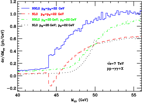
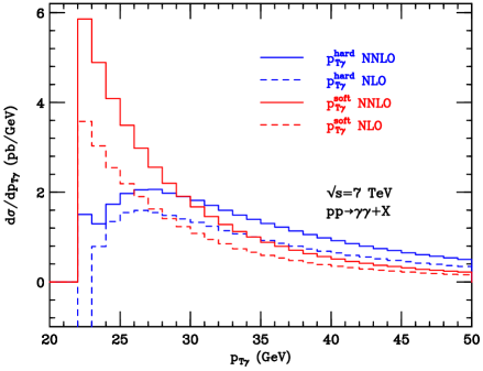
Figure 20: Left panel: the differential cross section $d\sigma/dM_{\gamma\gamma}$ in two configurations with symmetric and asymmetric photon $p_{T}$ cuts. NLO (red dashed) and NNLO (blue solid) results with symmetric cuts ($p_{H}=p_{S}=22$ GeV) and NLO (black dotted) and NNLO (green dash-dotted) results with asymmetric cuts ($p_{H}=25$ GeV, $p_{S}=22$ GeV). Right panel: NLO (dashed) and NNLO (solid) results for the differential cross sections $d\sigma/dp_{T\gamma}^{hard}$ (blue) and $d\sigma/dp_{T\gamma}^{soft}$ (red) of the harder and softer photon in the configuration with symmetric $p_{T}$ cuts, $\,p_{H}=p_{S}=22$ GeV.

In Fig. 20-left we report the results for $d\sigma/dM_{\gamma\gamma}$ in the $M_{\gamma\gamma}$ region that is close to the LO threshold at $M_{\gamma\gamma}=M^{LO}_{\rm dir}$. For comparison, we present the results for two different configurations with asymmetric ($p_{H}=25~{}{\rm GeV},\,p_{S}=22~{}{\rm GeV}$) and symmetric ($p_{H}=p_{S}=22~{}{\rm GeV}$) $p_{T}$ cuts. We remark that the two results are obtained by only varying the value of $p_{H}$, while all the other kinematical cuts and parameters of the calculation are unchanged.

We first briefly comment on the case with asymmetric $p_{T}$ cuts. The NLO and NNLO results in Fig. 20-left exactly correspond to those in Figs. 11-left and 17-left, the only difference being the much smaller $M_{\gamma\gamma}$ bin size, which is equal to 0.2 GeV. The behaviour of the LO and NLO results for $d\sigma/dM_{\gamma\gamma}$ has been discussed in detail at the end of Sect. 2.3.3 (see Fig. 10). In particular, the LO result has a threshold at $M_{\gamma\gamma}=M^{LO}_{\rm dir}=50$ GeV and the NLO result has an upward double-side cusp at $M_{\gamma\gamma}=M^{LO}_{\rm dir}$. The NLO cusp behaviour is due to soft-gluon radiation effects [60]. The ‘unphysical’ soft-gluon effects persist at the NNLO level and their dominant (at the formal level) contribution leads to a negative double-logarithmic enhancement ($\propto-\ln^{2}(\epsilon_{M})$) of the NLO cusp behaviour in Eq. (35). This double-logarithmic contribution produces a downward double-side cusp in the NNLO result at $M_{\gamma\gamma}=M^{LO}_{\rm dir}$. The NNLO cusp is very narrow and its effect is (partly) smeared by the bin size in the results of Fig. 20-left. Nonetheless, this effect is still visible in Fig. 20-left since the shapes of the NLO and NNLO results are quite different in the vicinity of $M_{\gamma\gamma}\sim 50$ GeV.

The shape of $d\sigma/dM_{\gamma\gamma}$ is quite different in the two configurations with asymmetric and symmetric $p_{T}$ cuts (Fig. 20-left). The LO result with symmetric $p_{T}$ cuts is not shown in Fig. 20-left. Its shape is exactly similar to that with asymmetric $p_{T}$ cuts (see Fig. 10 and Eq. (34)) since the value of $p_{S}$ does not matter at the LO and, in particular, $d\sigma^{LO}/dM_{\gamma\gamma}$ has its threshold at $M_{\gamma\gamma}=M^{LO}_{\rm dir}=44$ GeV (since $p_{H}=22$ GeV). In the case of symmetric $p_{T}$ cuts, the NLO and NNLO values of $d\sigma/dM_{\gamma\gamma}$ are quite small below the LO threshold. Just above the LO threshold ($M_{\gamma\gamma}\raisebox{-2.58334pt}{\hbox to0.0pt{$\,\sim\,$\hss}}\raisebox{1.72218pt}{$\,>\,$}M^{LO}_{\rm dir}$), the NLO result is (relatively) large and negative and the NNLO result is also (relatively) large but positive. This NLO behaviour is unphysical. In particular, the relatively-large and negative differential cross section $d\sigma^{NLO}/dM_{\gamma\gamma}$ at $M_{\gamma\gamma}\sim 44$ GeV ‘explains’ the unphysical behaviour of the NLO total cross section at $\Delta p_{T}=0$. In the case of symmetric (or nearly-symmetric) $p_{T}$ cuts $d\sigma^{NLO}/dM_{\gamma\gamma}$ becomes negative at $M_{\gamma\gamma}\sim M^{LO}_{\rm dir}$ and, after integration over $M_{\gamma\gamma}$, this negative contribution is responsible for the decreasing behaviour (see Fig. 19-right) of the NLO total cross section at small values of $\Delta p_{T}$ ($0\raisebox{-2.58334pt}{\hbox to0.0pt{$\,\sim\,$\hss}}\raisebox{1.72218pt}{$\,<\,$}\Delta p_{T}\raisebox{-2.58334pt}{\hbox to0.0pt{$\,\sim\,$\hss}}\raisebox{1.72218pt}{$\,<\,$}1$ GeV). We note that also $d\sigma/dM_{\gamma\gamma}$ (and not only the total cross section) for symmetric $p_{T}$ cuts is physically expected to be larger than the corresponding differential cross section for asymmetric $p_{T}$ cuts. This physical expectation is not fulfilled by the NLO results of Fig. 20-left in the regions where $44~{}{\rm GeV}\raisebox{-2.58334pt}{\hbox to0.0pt{$\,\sim\,$\hss}}\raisebox{1.72218pt}{$\,<\,$}M_{\gamma\gamma}\raisebox{-2.58334pt}{\hbox to0.0pt{$\,\sim\,$\hss}}\raisebox{1.72218pt}{$\,<\,$}45.4~{}{\rm GeV}$ and $M_{\gamma\gamma}\sim 50$ GeV (although both differential cross sections have a positive value at $M_{\gamma\gamma}\sim 45.4~{}{\rm GeV}$ and $M_{\gamma\gamma}\sim 50$ GeV).

Despite their apparent shape difference, the fixed-order behaviour of $d\sigma/dM_{\gamma\gamma}$ at $M_{\gamma\gamma}\sim M^{LO}_{\rm dir}$ for asymmetric and symmetric $p_{T}$ cuts is produced by the same underlying mechanism [60], as we are going to discuss below. In this sense, the unphysical fixed-order behaviour of the total cross section at $p_{H}\simeq p_{S}$ can also be regarded as a consequence (after integration) of unphysical soft-gluon effects for non-smooth differential distributions [60] (e.g., $d\sigma/dM_{\gamma\gamma}$ and, also, $d\sigma/dp_{T\gamma}^{hard}$ and $d\sigma/dp_{T\gamma}^{soft}$ as discussed below).

Analogously to the case of asymmetric $p_{T}$ cuts (see Eq. (35)), in the case of symmetric $p_{T}$ cuts we have examined the NLO shape of $d\sigma/dM_{\gamma\gamma}$ at $M_{\gamma\gamma}\sim M^{LO}_{\rm dir}$ in analytic form, and we find the dominant behaviour

$$\frac{d\sigma^{NLO}}{dM_{\gamma\gamma}}=b_{0}-{\sqrt{\epsilon_{M}}}\;b_{(+)}\,\ln^{2}\left(\frac{1}{\epsilon_{M}}\right)\Theta(M_{\gamma\gamma}-M^{LO}_{\rm dir})+\;\dots\;,\quad\quad(p_{H}=p_{S},M_{\gamma\gamma}\sim M^{LO}_{\rm dir})\;,$$ (40)

where $b_{0}$ and $b_{(+)}$ are positive constants (i.e., they do not depend on $M_{\gamma\gamma}$) and the dots in the right-hand side denote subdominant contributions in the limit $M_{\gamma\gamma}\rightarrow M^{LO}_{\rm dir}$. According to Eq. (40), $d\sigma^{NLO}/dM_{\gamma\gamma}$ is finite at $M_{\gamma\gamma}=M^{LO}_{\rm dir}$. Its behaviour just above the LO threshold ($M_{\gamma\gamma}>M^{LO}_{\rm dir}$) is analogous to that in Eq. (35) and, in particular, the first derivative of $d\sigma^{NLO}/dM_{\gamma\gamma}$ with respect to $M_{\gamma\gamma}$ (i.e., the slope of $d\sigma^{NLO}/dM_{\gamma\gamma}$) diverges to $-\infty$. Therefore, $d\sigma^{NLO}/dM_{\gamma\gamma}$ has an upward cusp at $M_{\gamma\gamma}=M^{LO}_{\rm dir}$. At variance with Eq. (35), the behaviour of the result in Eq. (40) is smooth just below the LO threshold ($M_{\gamma\gamma}<M^{LO}_{\rm dir}$) and, in particular, the slope of $d\sigma^{NLO}/dM_{\gamma\gamma}$ is finite (subdominant terms of ${\cal O}(\epsilon_{M})$ are neglected in the right-hand side of Eq. (40)) in this $M_{\gamma\gamma}$ region. Therefore, $d\sigma^{NLO}/dM_{\gamma\gamma}$ has a single-side cusp at $M_{\gamma\gamma}=M^{LO}_{\rm dir}$ (rather than a double-side cusp as in the case of asymmetric $p_{T}$ cuts).

The NLO quantitative results in Fig. 20-left for the symmetric $p_{T}$ cut configuration are consistent with the analytic behaviour in Eq. (40). We also note (Fig. 20-left) that the NLO value of $d\sigma/dM_{\gamma\gamma}$ at $M_{\gamma\gamma}=M^{LO}_{\rm dir}=44$ GeV is very small and, in particular, this implies that $b_{0}$ in Eq. (40) is much smaller than $a_{0}$ in Eq. (35). This is not unexpected since in the case of symmetric $p_{T}$ cuts ($p_{H}=p_{S}$) the LO threshold $M^{LO}_{\rm dir}$ and the ‘approximate’ threshold $M^{LO}$ for hard radiation (see Eq. (22)) actually coincides. As a consequence of the small value of $b_{0}$, the upward single-side cusp drives $d\sigma^{NLO}/dM_{\gamma\gamma}$ to negative values in the region just above the LO threshold. By further increasing $M_{\gamma\gamma}$, the physical (positive) behaviour of $d\sigma/dM_{\gamma\gamma}$ sets in and, consequently, $d\sigma^{NLO}/dM_{\gamma\gamma}$ has a local minimum (with a negative value) in the vicinity of $M^{LO}_{\rm dir}$.

The NLO behaviours in Eqs. (35) and (40) (though they are partly different) are directly related. Indeed, they are both due to the non-smooth behaviour of $d\sigma^{LO}/dM_{\gamma\gamma}$ at $M_{\gamma\gamma}=M^{LO}_{\rm dir}$ that produces an unbalance between real and virtual soft-gluon effects at higher perturbative orders [60]. The mechanism that leads to both Eqs. (35) and (40) is analogous (see the discussion that accompanies Eq. (35) in Sect. 2.3.3) and the main important difference regards the role of the real soft-emission contribution in the process of Eq. (36) (owing to transverse-momentum conservation the one-loop virtual contribution to the process $q{\bar{q}}\rightarrow\gamma\gamma$ is independent of the value of $p_{S}$ and, consequently, it is insensitive to the difference between asymmetric and symmetric $p_{T}$ cuts). The radiated soft gluon produces a transverse-momentum unbalance ($p_{T\gamma}^{hard}\neq p_{T\gamma}^{soft}$) between the two photons and it can preferably lead to either a decrease of $p_{T\gamma}^{soft}$ or an increase of $p_{T\gamma}^{hard}$ with respect to the LO configuration ($p_{T\gamma}^{hard}=p_{T\gamma}^{soft}=p_{H}$) depending on the phase space that is available in the presence of the photon $p_{T}$ cuts. In the case of asymmetric $p_{T}$ cuts and $M_{\gamma\gamma}\sim M^{LO}_{\rm dir}$, the soft-gluon momentum recoil is ‘absorbed’ by the softer photon (i.e., the value of $p_{T\gamma}^{soft}$ decreases below its LO value $p_{T\gamma}^{soft}=p_{H}$, whereas $p_{T\gamma}^{hard}\simeq p_{H}$) and this produces diphoton events with $M_{\gamma\gamma}<M^{LO}_{\rm dir}$ (see the accompanying comments to Eq. (36)). In the case of symmetric $p_{T}$ cuts, the momentum $p_{T\gamma}^{soft}$ of the softer photon cannot decrease since it is always constrained to be larger than $p_{H}=p_{S}$ (as in an LO configuration) and, consequently, the soft-gluon momentum recoil is necessarily ‘absorbed’ by the harder photon. The momentum $p_{T\gamma}^{hard}$ tends to increase above its threshold value $p_{H}$ ($p_{T\gamma}^{hard}>p_{H}$), whereas $p_{T\gamma}^{soft}\simeq p_{H}$, and this leads to diphoton events with $M_{\gamma\gamma}>M^{LO}_{\rm dir}$. Therefore, below the LO threshold ($M_{\gamma\gamma}<M^{LO}_{\rm dir}$) there are no dominant real and virtual soft-gluon effects (here $d\sigma^{NLO}/dM_{\gamma\gamma}$ is smooth since it only receives contributions from hard radiation), whereas just above the LO threshold ($M_{\gamma\gamma}>M^{LO}_{\rm dir}$) virtual soft-gluon effects dominate since real soft-gluon radiation tends to produce diphoton events that are sufficiently far from $M_{\gamma\gamma}=M^{LO}_{\rm dir}$. This real–virtual kinematical mismatch produces the NLO double-logarithmic enhancement (see Eq. (40)) of the non-smooth behaviour of $d\sigma/dM_{\gamma\gamma}$ at $M_{\gamma\gamma}\raisebox{-2.58334pt}{\hbox to0.0pt{$\,\sim\,$\hss}}\raisebox{1.72218pt}{$\,>\,$}M^{LO}_{\rm dir}$.

In the case of symmetric $p_{T}$ cuts, the single-side cusp behaviour of $d\sigma/dM_{\gamma\gamma}$ at $M_{\gamma\gamma}\sim M^{LO}_{\rm dir}$ occurs at each perturbative order. Just above the LO threshold the slope of $d\sigma/dM_{\gamma\gamma}$ alternatively diverges to $+\infty$ or $-\infty$ at subsequent perturbative orders [60]. This non-smooth order-by-order behaviour is removed by all-order-resummation of soft-gluon effects [60]. After resummation, $d\sigma/dM_{\gamma\gamma}$ rapidly increases just above the LO threshold but it has a finite slope at $M_{\gamma\gamma}\sim M^{LO}_{\rm dir}$. In the context of fixed-order calculations, the unphysical shape of $d\sigma/dM_{\gamma\gamma}$ at $M_{\gamma\gamma}\sim M^{LO}_{\rm dir}$ is localized in a mass region whose size tends to decrease by increasing the perturbative order. This is consistent with the results in Fig. 20-left. At the NNLO the behaviour of $d\sigma/dM_{\gamma\gamma}$ is qualitatively consistent with physical expectations, with the sole exception of a narrow region very close to $M_{\gamma\gamma}=44$ GeV, where the divergent (to $+\infty$) slope of $d\sigma^{NNLO}/dM_{\gamma\gamma}$ produces an excess of diphoton events that is eventually also responsible for the (quantitatively small) unphysical (increasing) behaviour of the NNLO total cross section as $\Delta p_{T}\rightarrow 0$ (Fig. 19-right).

We comment on the results in Fig. 20-right for the transverse-momentum spectra $d\sigma/dp_{T\gamma}^{soft}$ and $d\sigma/dp_{T\gamma}^{hard}$ of the softer and harder photon. At the LO we have $p_{T\gamma}^{soft}=p_{T\gamma}^{hard}$ (because of transverse-momentum conservation) and the two spectra are identical. The LO spectrum (it is not shown in Fig. 20-right) monotonically decreases in going from the ‘kinematical’ (due to the $p_{T}$ cuts) lower limit at $p_{T\gamma}=p_{H}$ toward higher values of $p_{T\gamma}$. In Fig. 20-right we show the NLO and NNLO spectra in the case of the symmetric $p_{T}$ cut configuration with $p_{H}=p_{S}=22$ GeV. We note that the shape of $d\sigma/dp_{T\gamma}^{soft}$ is qualitatively unchanged by increasing the perturbative order, in agreement with the expected physical behaviour. The NLO and NNLO results for $d\sigma/dp_{T\gamma}^{hard}$ are instead definitely unphysical in the region that is close to the lower limit $p_{T\gamma}^{hard}=p_{H}$. In particular, $d\sigma^{NLO}/dp_{T\gamma}^{hard}$ is negative in the first bin closest to $p_{T\gamma}^{hard}=p_{H}=22$ GeV. This unphysical behaviour is due to the same soft-gluon effects that we have previously discussed in the context of the near-threshold behaviour of $d\sigma/dM_{\gamma\gamma}$. In the case of symmetric $p_{T}$ cuts, the real soft-gluon emission process in Eq. (36) mostly affects the transverse-momentum recoil of the harder photon and the value of $p_{T\gamma}^{hard}$ tends to increase above its lower limit at $p_{H}=22$ GeV. Therefore, in the region where $p_{T\gamma}^{hard}\simeq p_{H}$, virtual soft-gluon effects tend to be unbalanced and this produces order-by-order perturbative instabilities of $d\sigma/dp_{T\gamma}^{hard}$. Actually, in the limit $p_{T\gamma}^{hard}\rightarrow p_{H}$, the NLO result for $d\sigma/dp_{T\gamma}^{hard}$ logarithmically diverges to $-\infty$ [60],

$$\frac{d\sigma^{NLO}}{dp_{T\gamma}^{hard}}\,\propto-\;\ln^{2}(p_{T\gamma}^{hard}-p_{S})\;\;,\quad\quad\quad\;\;\;\quad(p_{T\gamma}^{hard}\rightarrow p_{H}=p_{S})\;\;,$$ (41)

and the NNLO result diverges to $+\infty$. This divergent behaviour is consistent with the NLO and NNLO results in Fig. 20-right (the local minimum of $d\sigma^{NNLO}/dp_{T\gamma}^{hard}$ in the second bin closest to 22 GeV is due to a numerical compensation between dominant and subdominant logarithmic contributions).

This divergent behaviour of $d\sigma/dp_{T\gamma}^{hard}$ is also consistent with the total cross section results in Fig. 19-right. Indeed, the total cross section can be obtained by integrating $d\sigma/dp_{T\gamma}^{hard}$ and, more specifically, the $\Delta p_{T}$-slope of the total cross section is directly related to the $p_{T}$ spectra of the photons. Independently of the perturbative order and of the value of the $p_{T}$ cuts, we have

$$\frac{\partial\,\sigma(p_{H},p_{S})}{\partial\,p_{H}}=-\;\left.\frac{d\sigma}{dp_{T\gamma}^{hard}}\,\right|_{p_{T\gamma}^{hard}=p_{H}}\;\;,\quad\quad\quad\;\;\;\quad(p_{T\gamma}^{soft}\geq p_{S})\;\;.$$ (42)

This relation shows that the $\Delta p_{T}$-slope of the total cross section with respect to variations of $p_{H}$ (e.g., provided $\Delta p_{T}>0$ in Fig. 19-right) is equal (but with the opposite sign) to the value of $d\sigma/dp_{T\gamma}^{hard}$. In particular, in the case of symmetric $p_{T}$ cuts the behaviours in Eqs. (39) and (41) are fully consistent with each other, since they are directly related throughout Eq. (42).

In the case of symmetric $p_{T}$ cuts, $p_{T\gamma}^{soft}$ is not directly sensitive to soft-gluon radiation in the region where $p_{T\gamma}^{soft}\simeq p_{H}=p_{S}$, and there is no evident sign of unphysical behaviour in the results of Fig. 20-right for $d\sigma/dp_{T\gamma}^{soft}$. In other words, the soft-gluon instabilities of $p_{T\gamma}^{hard}$ are smeared by the integration over $p_{T\gamma}^{hard}$ in the fixed-order computation of $d\sigma/dp_{T\gamma}^{soft}$.

As we have discussed in our comments on the behaviour of $d\sigma/dM_{\gamma\gamma}$ at $M_{\gamma\gamma}\sim M^{LO}_{\rm dir}$, the LO kinematical configuration with $p_{T\gamma}^{soft}=p_{T\gamma}^{hard}=p_{H}$ is highly sensitive to soft-gluon effects and, in going from symmetric to asymmetric $p_{T}$ cut configurations the transverse momenta of the harder and softer photon exchange their role with respect to soft-gluon sensitivity. Therefore, in the case of asymmetric $p_{T}$ cuts, we expect [60] an evident unphysical behaviour of $d\sigma/dp_{T\gamma}^{soft}$ (rather than $d\sigma/dp_{T\gamma}^{hard}$).

This expectation is confirmed by the results for $d\sigma/dp_{T\gamma}^{soft}$ and $d\sigma/dp_{T\gamma}^{hard}$ that are presented in Fig. 2 of Ref. [35] (they refer to the asymmetric $p_{T}$ cut configuration with $p_{H}=40$ GeV and $p_{S}=25$ GeV). The NLO and NNLO results for $d\sigma/dp_{T\gamma}^{soft}$ in Fig. 2-right of Ref. [35] show perturbative instabilities in the region where $p_{T\gamma}^{soft}\simeq p_{H}=40$ GeV. In particular, the LO result for $d\sigma/dp_{T\gamma}^{soft}$ has an unphysical threshold at $p_{T\gamma}^{soft}=p_{H}$ and, therefore [35], the NLO result has the double-logarithmic divergent behaviour $d\sigma^{NLO}/dp_{T\gamma}^{soft}\propto+\;\ln^{2}(p_{H}-p_{T\gamma}^{soft})$ if $p_{T\gamma}^{soft}$ tends to $p_{H}$ in the region where $p_{T\gamma}^{soft}<p_{H}$. Analogously to the case of Eq. (41) for symmetric $p_{T}$ cuts, this divergent behaviour of $d\sigma^{NLO}/dp_{T\gamma}^{soft}$ for asymmetric $p_{T}$ cuts is directly related to the unphysical behaviour of the total cross section with nearly-symmetric $p_{T}$ cuts. Indeed, we have

$$\frac{\partial\,\sigma(p_{H},p_{S})}{\partial\,p_{S}}=-\;\left.\frac{d\sigma}{dp_{T\gamma}^{soft}}\,\right|_{p_{T\gamma}^{soft}=p_{S}}\;\;,\quad\quad\quad\;\;\;\quad(p_{H}>p_{S})\;\;,$$ (43)

and this equation relates the value of $d\sigma/dp_{T\gamma}^{soft}$ to the $\Delta p_{T}$-slope of the total cross section of Fig. 19-right in the region where $\Delta p_{T}<0$. In particular, by using Eqs. (39) and (43), the divergent behaviour of $d\sigma^{NLO}/dp_{T\gamma}^{soft}$ if $p_{T\gamma}^{soft}\rightarrow p_{H}$ with $p_{S}<p_{H}$ is fully consistent with the NLO behaviour of the $\Delta p_{T}$-slope of the total cross section with nearly-symmetric $p_{T}$ cuts and $\Delta p_{T}<0$. Analogously to the case of other soft-gluon sensitive observables, the perturbative instabilities of $d\sigma^{NLO}/dp_{T\gamma}^{soft}$ for asymmetric $p_{T}$ cuts can be removed by performing all-order soft-gluon resummation [43].

The unphysical fixed-order behaviour of the total cross section for nearly-symmetric $p_{T}$ cuts obviously affects also the behaviour of related differential cross sections. Various differential cross sections are affected in different ways. The results in Fig. 20 show that $d\sigma/dM_{\gamma\gamma}$ and $d\sigma/dp_{T\gamma}^{hard}$ have evident unphysical behaviour in limited regions of $M_{\gamma\gamma}$ and $p_{T\gamma}^{hard}$, respectively. In the case of $d\sigma/d\cos\theta^{*}$ we expect ‘unphysical’ effects of normalization (and, possibly, shape) in the region of central values of $\cos\theta^{*}$, which is mostly sensitive to the $M_{\gamma\gamma}$ region that is relatively close to $M^{LO}_{\rm dir}$. The case of the differential cross section $d\sigma/dp_{T\gamma}^{soft}$ in the region where $p_{T\gamma}^{soft}>p_{H}$ is somehow ‘special’, since its fixed-order results do not show evident signs of unphysical behaviour (Fig. 20-right). However, the integral of $d\sigma/dp_{T\gamma}^{soft}$ over the region with $p_{T\gamma}^{soft}\geq p_{T}^{{\rm min}}$ exactly corresponds to the total cross section in a configuration of symmetric $p_{T}$ cuts with $p_{H}=p_{S}=p_{T}^{{\rm min}}$. Since the fixed-order result of such total cross section is unphysical, it turns out that the overall normalization (independently of the detailed shape) of $d\sigma/dp_{T\gamma}^{soft}$ is sensitive to soft-gluon perturbative instabilities at all values of $p_{T\gamma}^{soft}$ with $p_{T\gamma}^{soft}>p_{H}$.

As discussed in Sect. 2.2 the NNLO results presented in this paper are affected by a systematic uncertainty related to the finite value of the parameter ($q_{T\rm cut}$ or $r_{\rm cut}$) that is used in the numerical implementation of the $q_{T}$ subtraction method. An estimate of these uncertainties for total cross sections is explicitly reported in the NNLO results presented in Table 2. At fixed value of $q_{T\rm cut}$ ($r_{\rm cut}$), the systematic uncertainties on differential cross sections tend to be larger than the corresponding uncertainties on fiducial (total) cross sections. Such uncertainties can be enhanced in the presence of soft-gluon instabilities (as in the case of observables that we have discussed in this subsection), since the instabilities are smeared by the finite value of $q_{T\rm cut}$ ($r_{\rm cut}$). More detailed studies are needed to assess the numerical precision of the NNLO results in these situations. Such studies, however, cannot improve the physical predictivity of the NNLO result, since the latter is affected by sizeable theoretical uncertainties produced by the same (unphysical) soft-gluon effects.

4 Summary

In this paper we have considered diphoton production in hadronic collisions at LHC energies and we have presented a study of QCD radiative corrections at NLO and NNLO. At NLO we have performed a thorough analysis of photon isolation and its perturbative QCD effects, comparing results obtained by using smooth cone and standard cone isolation. While the former facilitates theoretical calculations by removing the fragmentation component (and the ensuing effects of the poorly-known non-perturbative fragmentation functions of the photon), the latter is the isolation criterion that is typically used in experimental analyses. We have then extended our study to NNLO, where only smooth cone isolation results can be presently obtained.

Our main results can be summarised as follows.

• We have shown that lowest-order results for diphoton production are affected by large radiative corrections at higher orders. The large radiative corrections are due to partonic subprocesses with high parton multiplicity in the final state. As a consequence, the radiative corrections are typically positive and they enhance diphoton production rates and related kinematical distributions. Since the final-state partons can be produced outside the photon isolation cones, it also follows that the large radiative corrections have a relatively-mild dependence on the photon isolation prescription. In particular, the quantitative differences between smooth and standard isolation tend to decrease upon the inclusion of radiative corrections.

• We have presented a detailed comparison of fiducial cross sections and differential distributions obtained within standard and smooth cone isolation at NLO. In the case of tight isolation ($E_{T\,{\rm max}}\sim$ few GeV) the comparison shows that the two isolation procedures lead to results that are consistent within the corresponding scale uncertainties. In the case of moderate isolation ($E_{T\,{\rm max}}\sim$ 10 GeV), the same features hold true for diphoton observables that are ‘effectively’ computed at NLO accuracy. In ‘effective’ LO regions (such as at small values of $M_{\gamma\gamma}$ or $\Delta\Phi_{\gamma\gamma}$) the two isolation procedures lead to NLO differences that are much smaller than the size of the NNLO corrections computed within smooth isolation. We thus conclude that the smooth cone isolation provides a consistent theoretical framework to compute radiative corrections up to NNLO and that, if photon isolation is sufficiently tight, the ensuing predictions can be reliably compared with experimental measurements carried out by using standard cone isolation with the same values of the isolation parameters ($E_{T\,{\rm max}}$ and cone isolation radius $R$).

• An alternative approximation scheme of standard cone isolation consists in complementing the NLO calculation of the direct component with the LO computation of the fragmentation component. We have shown that such a scheme features an unphysical NLO dependence on $E_{T\,{\rm max}}$ and, therefore, it is not recommended.

• The NNLO computation of fiducial and differential cross sections shows that the NNLO corrections are rather large in the phase space regions where the calculation is an ‘effective’ NNLO prediction. The impact of the NNLO corrections can become huge in phase space regions where the calculation is ‘effectively’ an NLO prediction, as for the cases of small values of $M_{\gamma\gamma}$, low values of $\Delta\Phi_{\gamma\gamma}$ and relatively-large values of $p_{T\gamma\gamma}$. We have also observed that NLO and NNLO uncertainties obtained through scale variations do not overlap. This is mainly due to the significant contribution of the $qg$ initial-state partonic channel, which, although parametrically suppressed by one power of $\alpha_{\mathrm{S}}$ with respect to the LO $q{\bar{q}}$ contribution, is enhanced by the large ${\cal L}_{qg}$ luminosity. As a consequence, the true theoretical uncertainty is larger than the one obtained by performing customary scale variations. A more reliable estimate of the perturbative uncertainties can be obtained by properly taking into account the differences between the NLO and NNLO results. For instance, the perturbative uncertainty at NNLO (NLO) can be defined as the half difference between the central scale predictions at NNLO (NLO) and NLO (LO).

• The comparison of the NNLO calculation to the experimental results shows a clear improvement with respect to NLO in the description of the LHC data. The data tend to overshoot the NNLO predictions but, if the perturbative uncertainty is properly taken into account, the LHC data are consistent with the NNLO results in both ‘effective’ NNLO and ‘effective’ NLO regions.

• We have discussed and remarked how diphoton rates and kinematical distributions are strongly affected by the selection cuts that are typically applied on the transverse momenta of the photons. These selection cuts also lead to unphysical thresholds and ensuing perturbative instabilities in the fixed-order computations of the $M_{\gamma\gamma}$ distribution, of the transverse-momentum spectra of the photons and of related observables. We have discussed the behaviour of the NLO and NNLO results in these threshold regions, by presenting the logarithmic structure of the perturbative instabilities in analytic form. The effect of the perturbative instabilities is tamed by considering sufficiently smeared observables. Such fixed-order perturbative instabilities can be eliminated only through a proper all-order resummation of the logarithmically-enhanced contributions.

Acknowledgements. We are very grateful to Eric Pilon and Jean-Philippe Guillet for their help with the program DIPHOX. LC would like to thank the INFN of Florence for kind hospitality, while parts of this project were carried out. This research was supported in part by Fondazione Cariplo under the grant number 2015-0761, by the Swiss National Science Foundation (SNF) under contract 200020-169041 and by the Research Executive Agency (REA) of the European Union under the Grant Agreement number PITN-GA-2012-316704 (Higgstools).

References

- [1] T. Aaltonen et al. [CDF Collaboration], Phys. Rev. D 84 (2011) 052006 [arXiv:1106.5131 [hep-ex]].
- [2] G. Aad et al. [ATLAS Collaboration], Phys. Rev. D 85 (2012) 012003 [arXiv:1107.0581 [hep-ex]].
- [3] S. Chatrchyan et al. [CMS Collaboration], JHEP 1201 (2012) 133 [arXiv:1110.6461 [hep-ex]].
- [4] G. Aad et al. [ATLAS Collaboration], JHEP 1301 (2013) 086 [arXiv:1211.1913 [hep-ex]].
- [5] T. Aaltonen et al. [CDF Collaboration], Phys. Rev. Lett. 110 (2013) 10, 101801 [arXiv:1212.4204 [hep-ex]].
- [6] V. M. Abazov et al. [D0 Collaboration], Phys. Lett. B 725 (2013) 6 [arXiv:1301.4536 [hep-ex]].
- [7] S. Chatrchyan et al. [CMS Collaboration], Eur. Phys. J. C 74 (2014) 11, 3129 [arXiv:1405.7225 [hep-ex]].
- [8] M. Aaboud et al. [ATLAS Collaboration], Phys. Rev. D 95 (2017) no.11, 112005 [arXiv:1704.03839 [hep-ex]].
- [9] G. Aad et al. [ATLAS Collaboration], Phys. Lett. B 716 (2012) 1 [arXiv:1207.7214 [hep-ex]].
- [10] S. Chatrchyan et al. [CMS Collaboration], Phys. Lett. B 716 (2012) 30 [arXiv:1207.7235 [hep-ex]].
- [11] V. Khachatryan et al. [CMS Collaboration], Eur. Phys. J. C 74 (2014) no.10, 3076 [arXiv:1407.0558 [hep-ex]].
- [12] G. Aad et al. [ATLAS Collaboration], Phys. Rev. D 90 (2014) no.11, 112015 [arXiv:1408.7084 [hep-ex]].
- [13] G. Aad et al. [ATLAS Collaboration], Phys. Lett. B 718 (2012) 411 [arXiv:1209.0753 [hep-ex]].
- [14] S. Chatrchyan et al. [CMS Collaboration], Phys. Lett. B 719 (2013) 42 [arXiv:1210.2052 [hep-ex]].
- [15] S. Chatrchyan et al. [CMS Collaboration], JHEP 1303 (2013) 111 [arXiv:1211.4784 [hep-ex]].
- [16] G. Aad et al. [ATLAS Collaboration], Phys. Rev. Lett. 113 (2014) no.17, 171801 [arXiv:1407.6583 [hep-ex]].
- [17] G. Aad et al. [ATLAS Collaboration], Phys. Rev. D 92 (2015) no.3, 032004 [arXiv:1504.05511 [hep-ex]].
- [18] V. Khachatryan et al. [CMS Collaboration], Phys. Lett. B 750 (2015) 494 [arXiv:1506.02301 [hep-ex]].
- [19] The ATLAS collaboration, “Search for resonances decaying to photon pairs in 3.2 fb-1 of collisions at = 13 TeV with the ATLAS detector,” ATLAS-CONF-2015-081.
- [20] CMS Collaboration, “Search for new physics in high mass diphoton events in proton-proton collisions at 13 TeV,” CMS-PAS-EXO-15-004.
- [21] CMS Collaboration, “Search for new physics in high mass diphoton events in of proton-proton collisions at and combined interpretation of searches at and ,” CMS-PAS-EXO-16-018.
- [22] M. Aaboud et al. [ATLAS Collaboration], JHEP 1609 (2016) 001 [arXiv:1606.03833 [hep-ex]].
- [23] V. Khachatryan et al. [CMS Collaboration], Phys. Rev. Lett. 117 (2016) no.5, 051802 [arXiv:1606.04093 [hep-ex]].
- [24] V. Khachatryan et al. [CMS Collaboration], Phys. Lett. B 767 (2017) 147 [arXiv:1609.02507 [hep-ex]].
- [25] M. Aaboud et al. [ATLAS Collaboration], Phys. Lett. B 775 (2017) 105 [arXiv:1707.04147 [hep-ex]].
- [26] S. Frixione, Phys. Lett. B 429 (1998) 369 [hep-ph/9801442].
- [27] J. Butterworth, G. Dissertori, S. Dittmaier, D. de Florian, N. Glover, K. Hamilton, J. Huston and M. Kado et al., “Les Houches 2013 Physics at TeV Colliders: Standard Model Working Group Report,” arXiv:1405.1067 [hep-ph].
- [28] T. Binoth, J. P. Guillet, E. Pilon and M. Werlen, Eur. Phys. J. C 16 (2000) 311 [hep-ph/9911340].
- [29] D. A. Dicus and S. S. D. Willenbrock, Phys. Rev. D 37 (1988) 1801.
- [30] Z. Bern, L. J. Dixon and C. Schmidt, Phys. Rev. D 66 (2002) 074018 [hep-ph/0206194].
- [31] J. M. Campbell, R. K. Ellis and C. Williams, JHEP 1107 (2011) 018 [arXiv:1105.0020 [hep-ph]].
- [32] V. D. Barger, T. Han, J. Ohnemus and D. Zeppenfeld, Phys. Rev. D 41 (1990) 2782; V. Del Duca, W. B. Kilgore and F. Maltoni, Nucl. Phys. B 566 (2000) 252 [hep-ph/9910253].
- [33] Z. Bern, L. J. Dixon and D. A. Kosower, Nucl. Phys. B 437 (1995) 259 [hep-ph/9409393]; A. Signer, Phys. Lett. B 357 (1995) 204 [hep-ph/9507442].
- [34] C. Anastasiou, E. W. N. Glover and M. E. Tejeda-Yeomans, Nucl. Phys. B 629 (2002) 255 [hep-ph/0201274].
- [35] S. Catani, L. Cieri, D. de Florian, G. Ferrera and M. Grazzini, Phys. Rev. Lett. 108 (2012) 072001 (Erratum: Phys. Rev. Lett. 117 (2016) 089901) [arXiv:1110.2375 [hep-ph]].
- [36] S. Catani and M. Grazzini, Phys. Rev. Lett. 98 (2007) 222002 [hep-ph/0703012].
- [37] J. M. Campbell, R. K. Ellis, Y. Li and C. Williams, JHEP 1607 (2016) 148 [arXiv:1603.02663 [hep-ph]].
- [38] R. Boughezal, C. Focke, X. Liu and F. Petriello, Phys. Rev. Lett. 115 (2015) 062002 [arXiv:1504.02131 [hep-ph]].
- [39] J. Gaunt, M. Stahlhofen, F. J. Tackmann and J. R. Walsh, JHEP 1509 (2015) 058 [arXiv:1505.04794 [hep-ph]].
- [40] R. Boughezal, J. M. Campbell, R. K. Ellis, C. Focke, W. Giele, X. Liu, F. Petriello and C. Williams, Eur. Phys. J. C 77 (2017) 7 [arXiv:1605.08011 [hep-ph]].
- [41] M. Grazzini, S. Kallweit and M. Wiesemann, report CERN-TH-2017-232 [arXiv:1711.06631 [hep-ph]].
- [42] C. Balazs, E. L. Berger, P. M. Nadolsky and C.-P. Yuan, Phys. Rev. D 76 (2007) 013009 [arXiv:0704.0001 [hep-ph]].
- [43] L. Cieri, F. Coradeschi and D. de Florian, JHEP 1506 (2015) 185 [arXiv:1505.03162 [hep-ph]].
- [44] V. Del Duca, F. Maltoni, Z. Nagy and Z. Trocsanyi, JHEP 0304 (2003) 059 [hep-ph/0303012].
- [45] T. Gehrmann, N. Greiner and G. Heinrich, JHEP 1306 (2013) 058 [Erratum-ibid. 1406 (2014) 076] [arXiv:1303.0824 [hep-ph]].
- [46] J. M. Campbell and C. Williams, Phys. Rev. D 89 (2014) 113001 [arXiv:1403.2641 [hep-ph]].
- [47] T. Gehrmann, N. Greiner and G. Heinrich, Phys. Rev. Lett. 111 (2013) 222002 [arXiv:1308.3660 [hep-ph]].
- [48] Z. Bern, L. J. Dixon, F. Febres Cordero, S. Hoeche, H. Ita, D. A. Kosower, N. A. Lo Presti and D. Maitre, report IPHT-T13-269 [arXiv:1312.0592 [hep-ph]], Phys. Rev. D 90 (2014) 5, 054004 [arXiv:1402.4127 [hep-ph]].
- [49] S. Badger, A. Guffanti and V. Yundin, JHEP 1403 (2014) 122 [arXiv:1312.5927 [hep-ph]].
- [50] D. Faeh and N. Greiner, report ZU-TH-19-17 [arXiv:1706.08309 [hep-ph]].
- [51] M. Grazzini, S. Kallweit, D. Rathlev and A. Torre, Phys. Lett. B 731 (2014) 204 [arXiv:1309.7000 [hep-ph]].
- [52] M. Grazzini, S. Kallweit and D. Rathlev, JHEP 1507 (2015) 085 [arXiv:1504.01330 [hep-ph]].
- [53] J. M. Campbell, T. Neumann and C. Williams, JHEP 1711 (2017) 150 [arXiv:1708.02925 [hep-ph]].
- [54] J. M. Campbell, R. K. Ellis and C. Williams, Phys. Rev. Lett. 118 (2017) 222001, [arXiv:1612.04333 [hep-ph]].
- [55] A. Bierweiler, T. Kasprzik and J. H. Kühn, JHEP 1312 (2013) 071 [arXiv:1305.5402 [hep-ph]].
- [56] M. Chiesa, N. Greiner, M. Schoenherr and F. Tramontano, report ZU–TH-20-17 [arXiv:1706.09022 [hep-ph]].
- [57] S. Catani, M. Fontannaz, J. P. Guillet and E. Pilon, JHEP 0205 (2002) 028 [hep-ph/0204023].
- [58] S. Frixione and W. Vogelsang, Nucl. Phys. B 568 (2000) 60 [hep-ph/9908387].
- [59] S. Catani, M. Dittmar, D. E. Soper, W. J. Stirling, S. Tapprogge, S. Alekhin, P. Aurenche and C. Balazs et al., In *Geneva 1999, Standard model physics (and more) at the LHC* 1-115 [hep-ph/0005025].
- [60] S. Catani and B. R. Webber, JHEP 9710 (1997) 005 [hep-ph/9710333].
- [61] T. Binoth et al. [SM and NLO Multileg Working Group Collaboration], “Les Houches 2009 Workshop on Physics at TeV Colliders,” arXiv:1003.1241 [hep-ph].
- [62] J. Alcaraz Maestre et al. [SM AND NLO MULTILEG and SM MC Working Groups Collaboration], “Les Houches 2011 Workshop on Physics at TeV Colliders,” arXiv:1203.6803 [hep-ph].
- [63] R. Blair, B. Brelier, F. Bucci, S. Chekanov, M. Stockton and M. Tripiana, report CERN-OPEN-2011-041 (2011).
- [64] M. Wielers, report CERN-ATL-PHYS-2002-004 (2002).
- [65] G. Abbiendi et al. [OPAL Collaboration], Eur. Phys. J. C 31 (2003) 491 [hep-ex/0305075].
- [66] C. Frye, M. Freytsis, J. Scholtz and M. J. Strassler, JHEP 1603 (2016) 171 [arXiv:1510.08451 [hep-ph]].
- [67] J. R. Andersen et al., “Les Houches 2015 Physics at TeV Colliders: Standard Model Working Group Report,” arXiv:1605.04692 [hep-ph].
- [68] J. C. Collins and D. E. Soper, Phys. Rev. D 16 (1977) 2219.
- [69] M. Grazzini, JHEP 0802 (2008) 043 [arXiv:0801.3232 [hep-ph]].
- [70] S. Catani, L. Cieri, G. Ferrera, D. de Florian and M. Grazzini, Phys. Rev. Lett. 103 (2009) 082001 [arXiv:0903.2120 [hep-ph]].
- [71] S. Catani, G. Ferrera and M. Grazzini, JHEP 1005 (2010) 006 [arXiv:1002.3115 [hep-ph]].
- [72] G. Ferrera, M. Grazzini and F. Tramontano, Phys. Rev. Lett. 107 (2011) 152003 [arXiv:1107.1164 [hep-ph]].
- [73] G. Ferrera, M. Grazzini and F. Tramontano, Phys. Lett. B 740 (2015) 51 [arXiv:1407.4747 [hep-ph]].
- [74] F. Cascioli, T. Gehrmann, M. Grazzini, S. Kallweit, P. Maierhöfer, A. von Manteuffel, S. Pozzorini, D. Rathlev, L. Tancredi and E. Weihs, Phys. Lett. B 735 (2014) 311 [arXiv:1405.2219 [hep-ph]];
- [75] M. Grazzini, S. Kallweit and D. Rathlev, Phys. Lett. B 750 (2015) 407 [arXiv:1507.06257 [hep-ph]].
- [76] T. Gehrmann, M. Grazzini, S. Kallweit, P. Maierhöfer, A. von Manteuffel, S. Pozzorini, D. Rathlev and L. Tancredi, Phys. Rev. Lett. 113 (2014) 21, 212001 [arXiv:1408.5243 [hep-ph]].
- [77] M. Grazzini, S. Kallweit, S. Pozzorini, D. Rathlev and M. Wiesemann, JHEP 1608 (2016) 140 [arXiv:1605.02716 [hep-ph]].
- [78] M. Grazzini, S. Kallweit, D. Rathlev and M. Wiesemann, Phys. Lett. B 761 (2016) 179 [arXiv:1604.08576 [hep-ph]], JHEP 1705 (2017) 139 [arXiv:1703.09065 [hep-ph]].
- [79] D. de Florian, M. Grazzini, C. Hanga, S. Kallweit, J. M. Lindert, P. Maierhf̈er, J. Mazzitelli and D. Rathlev, JHEP 1609 (2016) 151 [arXiv:1606.09519 [hep-ph]]; M. Grazzini, G. Heinrich, S. Jones, S. Kallweit, M. Kerner, J. M. Lindert and J. Mazzitelli, report CERN-TH-2018-044 [arXiv:1803.02463 [hep-ph]].
- [80] H. T. Li and J. Wang, Phys. Lett. B 765 (2017) 265 [arXiv:1607.06382 [hep-ph]]; H. T. Li, C. S. Li and J. Wang, arXiv:1710.02464 [hep-ph].
- [81] R. Bonciani, S. Catani, M. Grazzini, H. Sargsyan and A. Torre, Eur. Phys. J. C 75 (2015) 581 [arXiv:1508.03585 [hep-ph]].
- [82] G. Bozzi, S. Catani, D. de Florian and M. Grazzini, Nucl. Phys. B 737 (2006) 73 [hep-ph/0508068].
- [83] S. Catani, L. Cieri, D. de Florian, G. Ferrera and M. Grazzini, Nucl. Phys. B 881 (2014) 414 [arXiv:1311.1654 [hep-ph]].
- [84] S. Catani and M. H. Seymour, Nucl. Phys. B 485 (1997) 291 [Erratum-ibid. B 510 (1998) 503] [hep-ph/9605323].
- [85] F. Cascioli, P. Maierhofer and S. Pozzorini, Phys. Rev. Lett. 108 (2012) 111601 [arXiv:1111.5206 [hep-ph]].
- [86] M. Becchetti and R. Bonciani, arXiv:1712.02537 [hep-ph].
- [87] S. Kawabata and H. Yokoya, Eur. Phys. J. C 77 (2017) no.5, 323 [arXiv:1607.00990 [hep-ph]].
- [88] P. Jain, S. Mitra, P. Sanyal and R. K. Verma, arXiv:1605.07360 [hep-ph].
- [89] P. Chiappetta, R. Fergani and J. P. Guillet, Z. Phys. C 69 (1996) 443.
- [90] S. Catani, M. Fontannaz, J. P. Guillet and E. Pilon, JHEP 1309 (2013) 007 [arXiv:1306.6498 [hep-ph]].
- [91] L. A. Harland-Lang, A. D. Martin, P. Motylinski and R. S. Thorne, Eur. Phys. J. C 75 (2015) 204 [arXiv:1412.3989 [hep-ph]].
- [92] L. Bourhis, M. Fontannaz and J. P. Guillet, Eur. Phys. J. C 2 (1998) 529 [arXiv:hep-ph/9704447].
- [93] T. Kaufmann, A. Mukherjee and W. Vogelsang, arXiv:1708.06683 [hep-ph].
- [94] L. E. Gordon and W. Vogelsang, Phys. Rev. D 50 (1994) 1901.
- [95] T. Binoth, J. P. Guillet, E. Pilon and M. Werlen, Phys. Rev. D 63 (2001) 114016 [hep-ph/0012191].
- [96] A. Gehrmann-De Ridder, E. W. N. Glover, Eur. Phys. J. C7 (1999) 29 [hep-ph/9806316].
- [97] M. L. Mangano et al., report CERN-TH-2016-112 [arXiv:1607.01831 [hep-ph]].
- [98] G. Bozzi, S. Catani, G. Ferrera, D. de Florian and M. Grazzini, Nucl. Phys. B 815 (2009) 174 [arXiv:0812.2862 [hep-ph]].
- [99] L. J. Cieri, arXiv:1207.3252 [hep-ph], in Proceedings of the 47th Rencontres de Moriond on QCD and High Energy Interactions, La Thuile, France, March 2012.
- [100] Durham HepData Project: see http://hepdata.cedar.ac.uk/view/ins1199269
- [101] S. Frixione and G. Ridolfi, Nucl. Phys. B 507 (1997) 315 [hep-ph/9707345].
- [102] A. Banfi and M. Dasgupta, JHEP 0401 (2004) 027 [hep-ph/0312108].