Imaginary potential in strongly coupled $\mathcal{N}=4$ SYM plasma in a magnetic field

Abstract

We study the effect of a constant magnetic field on the imaginary part of a quarkonia potential in a strongly-coupled $\mathcal{N}=4$ SYM plasma. We consider the pair axis to be aligned perpendicularly and parallel to the magnetic field, respectively. For both cases, we find that the presence of the magnetic field tends to enhance the imaginary potential thus decreasing the the thermal width. In addition, the magnetic field has a stronger effect on the imaginary potential when the pair axis is perpendicular to the magnetic field rather than parallel.

I Introduction

The heavy ion collisions at RHIC and LHC have produced a new state of matter so-called quark gluon plasma (QGP) JA ; KA ; EV . One experimental signal for QGP formation is dissociation of quarkonia . It was suggested earlier that the main mechanism responsible for this suppression is color screening TMA . But recently some authors argued that the imaginary part of the potential, ImV_QQ, may be a more important reason than screening ML ; AB ; NB ; MAE . Subsequently, this quantity has been studied in weakly coupled theories, see e.g. NB1 ; AD ; MM ; VC . However, much experiment data indicates that QGP is strongly coupled EV , so it would be interesting to study the imaginary potential in strongly coupled theories with the aid of nonpetubative methods. Such methods are now available via the AdS/CFT correspondence Maldacena:1997re ; Gubser:1998bc ; MadalcenaReview .

AdS/CFT, the duality between a string theory in AdS space and a conformal field theory in the physical space-time, has yielded many important insights for studying different aspects of QGP JCA . In this approach, Noronha and Dumitru have studied the imaginary potential of quarkonia for $\mathcal{N}=4$ SYM theory in their seminal work JN . Therein, the ImV_QQ is related to the effect of thermal fluctuations due to the interactions between the heavy quarks and the medium. After JN , there were many attempts to address ImV_QQ in this direction, for instance, the ImV_QQ of static quarkonia is studied in JN1 ; KB . The effect of velocity on ImV_QQ is discussed in JN2 ; MAL . The finite ’t Hooft coupling corrections on ImV_QQ is analyzed in KB1 . The influence of chemical potential on ImV_QQ is investigated in ZQ . For study of ImV_QQ in some AdS/QCD models, see NR ; JS . Moreover, there are other ways to study ImV_QQ from AdS/CFT, see JLA ; THA .

Recently, there are various observables or quantities that have been studied in strongly coupled $\mathcal{N}=4$ SYM plasma under the influence of a magnetic field, such as entropy density ED , conductivity KAMA , shear viscosity to entropy density ratio RCR , heavy quark potential RRO , drag force KIM and jet quenching parameter SLI . Motivated by this, in this paper we study the effect of a constant magnetic field on the imaginary part of heavy quarkonia potential in a strongly-coupled $\mathcal{N}=4$ SYM plasma. Specifically, we would like to see how a constant magnetic field affects ImV_QQ in this case. This is the purpose of the present work.

The rest of the paper is as follows. In the next section, we briefly review the background metric in the presence of a magnetic field given in ED . In section 3, we introduce the numerical procedure and show some numerical solutions. In section 4, we study the effect of a magnetic field on the imaginary potential for the pair axis to be aligned perpendicularly and parallel to the magnetic field, in turn. The last part is devoted to conclusion and discussion.

II magnetic brane background

Let us begin with a briefly review of the holographic dual of $\mathcal{N}=4$ SYM theory in the presence of a magnetic field ED . The holographic model is Einstein gravity coupled with a Maxwell field, corresponding to strongly coupled $\mathcal{N}=4$ SYM subjected to a constant and homogenous magnetic field. The bulk action is given by

$$S=\frac{1}{16\pi G_{5}}\int d^{5}x\sqrt{-g}(R+\frac{12}{L^{2}}-F^{2})+S_{body},$$ (1)

where $G_{5}$ denotes the 5-dimensional gravitational constant, $L$ stands for the radius of the asymptotic $AdS_{5}$ spacetime. $F$ refers to the Maxwell field strength 2-form. The boundary term $S_{body}$ contains the Chern-Simons terms, Gibbons-Hawking terms and other contributions necessary for a well posed variational principle, but all of them do not affect the solutions considered here ED .

The equations of motion obtained from (1) are

$$R_{\mu\nu}+\frac{4}{L^{2}}g_{\mu\nu}+\frac{1}{3}F_{\rho\sigma}F^{\rho\sigma}g_{\mu\nu}-2F_{\mu\rho}F_{\nu}^{\rho}=0,$$ (2)

and the Maxwell’s field equations

$$\nabla_{\mu}F^{\mu\nu}=0.$$ (3)

For simplicity, we set $L=1$ from now on. Then a general ansatz for the magnetic brane geometry can be written as

$$ds^{2}=-H(r)dt^{2}+e^{2P(r)}(dx^{2}+dy^{2})+e^{2K(r)}dz^{2}+\frac{dr^{2}}{H(r)},$$ (4)

with

$$F=Bdx\wedge dy,$$ (5)

where the boundary is located at $r=\infty$ and the horizon is located at $r=r_{h}$ with $H(r_{h})=0$. The constant $B$ stands for the bulk magnetic field, oriented along the $z$ direction. Also, $H(r)$, $P(r)$ and $K(r)$ can be determined by solving the equations of motion.

From (4), the equations of motion read

$$H(P^{\prime\prime}-K^{\prime\prime})+(H^{\prime}+H(2P^{\prime}+K^{\prime}))(P^{\prime}-K^{\prime})=-2B^{2}e^{-4P},$$ (6)

$$2P^{\prime\prime}+K^{\prime\prime}+2(P^{\prime})^{2}+(K^{\prime})^{2}=0,$$ (7)

$$\frac{1}{2}H^{\prime\prime}+\frac{1}{2}H^{\prime}(2P^{\prime}+K^{\prime})=4+\frac{2}{3}B^{2}e^{-4P},$$ (8)

$$2H^{\prime}P^{\prime}+H^{\prime}K^{\prime}+2H(P^{\prime})^{2}+4HP^{\prime}K^{\prime}=12-2B^{2}e^{-4P},$$ (9)

where $H\equiv H(r)$, $P\equiv P(r)$, $K\equiv K(r)$ and the derivations are with respect to $r$. For the above equations, one can check that with $B=0$, the solution reduces to that of $AdS_{5}$, represented by $H=e^{2P}=e^{2K}=r^{2}$. While for non-zero $B$, one finds an exact solution in the asymptotic IR regime, represents the product of a BTZ black hole times a two dimensional tours $T^{2}$ in the spatial directions orthogonal to the magnetic field (the $x,y$ directions are compact), as

$$ds^{2}=-3(r^{2}-r_{h}^{2})dt^{2}+\frac{B}{\sqrt{3}}(dx^{2}+dy^{2})+3r^{2}dz^{2}+\frac{dr^{2}}{3(r^{2}-r_{h}^{2})}.$$ (10)

It should be noticed that the metric (10) is valid only near the horizon ($r\sim r_{h}$), where the scale is much smaller than the magnetic field, $r\ll\sqrt{B}/3$, and recently some authors have used it to study the effect of a strong magnetic field on the drag force KIM and jet quenching parameter SLI .

However, when discuss the effect of a general magnetic field, not restricted to a strong magnetic field (or in the IR regime), one should use a solution that interpolates between (10) at small $r$ and $AdS_{5}$ at large $r$. As discussed in ED , this represents an RG flow between a $D=3+1$ CFT in the infrared and a $D=1+1$ CFT in the ultraviolet. Unfortunately, no analytic solution can be found in this case. Therefore, one needs to turn to numerical methods. In the next section, we will follow the argument in ED to present the numerical procedure.

III Numerical solutions

To begin with, we derive some useful equations. After eliminating the $B^{2}e^{-4P}$ terms in (6)$-$(9), we have

$$3H^{\prime\prime}+5(K^{\prime}+2P^{\prime})H^{\prime}+4({P^{\prime}}^{2}+2P^{\prime}K^{\prime})H-48=0,$$ (11)

$$3HP^{\prime\prime}+2H{P^{\prime}}^{2}-H^{\prime}P^{\prime}-5HP^{\prime}K^{\prime}+12-2H^{\prime}K^{\prime}=0,$$ (12)

$$3HK^{\prime\prime}+3H{K^{\prime}}^{2}+4H^{\prime}K^{\prime}+10HP^{\prime}K^{\prime}+2H{P^{\prime}}^{2}+2H^{\prime}P^{\prime}-24=0,$$ (13)

before solving the above equations, it is convenient to rescale the radial coordinates as follows ED : First, we rescale $t$ and $r$ as $r\rightarrow\bar{r}$ and $t\rightarrow\bar{t}$, and fix the horizon at $\bar{r}_{h}=1$, so that

$$H(1)=0,\qquad H^{\prime}(1)=1.$$ (14)

In this case, the Hawking temperature is given by

$$T=\frac{\sqrt{-g^{\prime}_{\bar{t}\bar{t}}g^{\bar{r}\bar{r}\prime}}}{4\pi}\big{|}_{\bar{r}=1}=\frac{1}{4\pi}.$$ (15)

Also, we rescale $x$, $y$, $z$ coordinates as

$$P(1)=K(1)=0,\qquad P^{\prime}(1)=4-\frac{b^{2}}{3},\qquad K^{\prime}(1)=4+\frac{b^{2}}{6},$$ (16)

where $b$ refers to the value of the magnetic field in the rescaled coordinates. Note that the second equation in (16) implies that, if one takes $b>2\sqrt{3}$, the term $P^{\prime}(1)$ will be negative, indicating that the geometry will not be asymptotically $AdS_{5}$. Therefore, we take $0\leq b<2\sqrt{3}$ here.

On the other hand, the geometry has the asymptotic behavior as $\bar{r}\rightarrow\infty$, so that

$$H(\bar{r})\rightarrow\bar{r}^{2},\qquad e^{2P(\bar{r})}\rightarrow m(b)\bar{r}^{2},\qquad e^{2K(\bar{r})}\rightarrow p(b)\bar{r}^{2},$$ (17)

where $m(b)$ and $p(b)$ are rescaling parameters which can be obtained numerically. In addition, the physical magnetic field $\mathcal{B}$ can be written as

$$\mathcal{B}=\sqrt{3}\frac{b}{m(b)}.$$ (18)

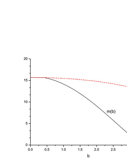
In fact, one can also derive the interval of $b$ from Eq.(18). One can numerically check that $m(b)$ is a decreasing function of $b$ and $m(b\rightarrow 2\sqrt{3})\rightarrow 0$ (see the left panel of fig.1). Thus, $b\in[0,2\sqrt{3})$ leads to $\mathcal{B}\in[0,\infty)$. Namely, one can cover in practice all values of $\mathcal{B}$ for $0\leq b<2\sqrt{3}$. Here it should be noticed that the actual $\mathcal{B}$ is immaterial, due to the presence of any other scale in the theory besides it. However, when switching on the temperature, this situation changes. In that case, one finds a new dimensionless scale given by $\mathcal{B}/T^{2}$ RRO . Therefore, one can tune the anisotropy in the imaginary potential by varying the value of the magnetic field.

Now we are ready to numerically solve the equations (11)$-$(13). For simplicity, we delete from now on the bars in the rescaled coordinates. The numerical procedures are as follows:

1). Choosing a value of $b$, one solves the coupled equations (11)$-$(13) with the conditions (14) and (16).

2). Fitting the asymptotic data for $e^{2P(r)}\rightarrow m(b)r^{2}$ and $e^{2K(r)}\rightarrow p(b)r^{2}$, one gets the values of $m(b)$ and $p(b)$. Meanwhile, the value of $\mathcal{B}$ is determined.

3). To go back to the original coordinates, one sets $(e^{2P(r)},e^{2K(r)})\rightarrow(e^{2P(r)}/m(b),e^{2K(r)}/p(b))$, after this, the numerical solutions can be obtained.

4). Likewise, one can discuss other cases by varying the value of $b$.

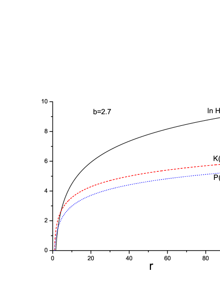
Here we present some numerical solutions. In the left panel of fig.1, we plot $m(b)$, $p(b)$ versus $b$, and we have checked that it matches the fig.1 in RCR . Also, in the right panel of fig.1, we plot $lnH(r)$, $K(r)$, $P(r)$ versus $r$ for $b=2.7$, and we find that it is completely consistent with the fig.3 in RRO .

Figure 1: Left: $p(b)$ (dash curve) and $m(b)$ (solid curve) versus $b$. Right: $lnH(r)$ (solid curve), $K(r)$ (dash curve) and $P(r)$ (dot curve) versus $r$ for $b=2.7$.

IV imaginary potential

Now we investigate the ImV_QQ of a heavy quarkonia for the background metric (4). Generally, to analyze the effect of a magnetic field, one needs to consider different orientations for the pair axis with respect to the magnetic field, i.e., transverse ($\theta=\pi/2$), parallel ($\theta=0$), and arbitrary direction ($\theta$). In this work, we study two extreme cases: $\theta=\pi/2$ and $\theta=0$.

IV.1 Transverse to the magnetic field ($\theta=\pi/2$)

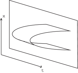
Considering the $Q\bar{Q}$ axis perpendicularly to the magnetic field in the $x$ direction, the coordinates are parameterized as

$$t=\tau,\qquad x=\sigma,\qquad y=0,\qquad z=0,\qquad r=r(\sigma),$$ (19)

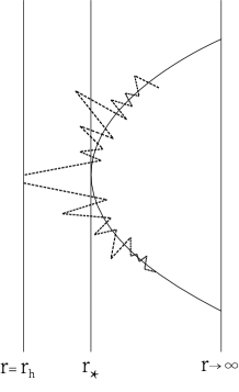
where the quark and anti-quark are located at $x=-\frac{D}{2}$ and $x=\frac{D}{2}$, respectively. Here $D$ is the inter-distance of $Q\bar{Q}$. The configuration of the string world-sheet is presented in fig.2.

To proceed, the string action is given by

$$S=-\frac{1}{2\pi\alpha^{\prime}}\int d\tau d\sigma\mathcal{L}=-\frac{1}{2\pi\alpha^{\prime}}\int d\tau d\sigma\sqrt{-g},$$ (20)

with $g$ the determinant of the induced metric and

$$g_{\alpha\beta}=g_{\mu\nu}\frac{\partial X^{\mu}}{\partial\sigma^{\alpha}}\frac{\partial X^{\nu}}{\partial\sigma^{\beta}},$$ (21)

where $g_{\mu\nu}$ and $X^{\mu}$ represent the metric and target space coordinates, respectively. The parameter $\alpha^{\prime}$ is related to ’t Hooft coupling as $1/\alpha^{\prime}=\sqrt{\lambda}$.

Substituting (19) into (4), the induced metric becomes

$$g_{00}=H(r),\qquad g_{01}=g_{10}=0,\qquad g_{11}=e^{2P(r)}+\frac{1}{H(r)}(\frac{dr}{d\sigma})^{2}.$$ (22)

Then one can identify the lagrangian density as

$$\mathcal{L}=\sqrt{H(r)e^{2P(r)}+(\frac{dr}{d\sigma})^{2}},$$ (23)

Notice that the action does not depend on $\sigma$ explicitly, so $\mathcal{L}$ satisfies

$$\mathcal{L}-\frac{\partial\mathcal{L}}{\partial(\frac{dr}{d\sigma})}\frac{dr}{d\sigma}=\frac{H(r)e^{2P(r)}}{\sqrt{H(r)e^{2P(r)}+(\frac{dr}{d\sigma})^{2}}}=constant.$$ (24)

Imposing the boundary condition at $\sigma=0$ (the deepest point of the U-shaped string),

$$\frac{dr}{d\sigma}=0,\qquad r=r_{*},$$ (25)

one finds

$$\frac{dr}{d\sigma}=\sqrt{\frac{a^{2}(r)-a(r)a(r_{*})}{a(r_{*})}},$$ (26)

with

$$a(r)=H(r)e^{2P(r)},\qquad a(r_{*})=H(r_{*})e^{2P(r_{*})}.$$ (27)

Integrating (26), the inter-distance of $Q\bar{Q}$ reads

$$D=2\int_{r_{*}}^{\infty}dr\frac{d\sigma}{dr}=2\int_{r_{*}}^{\infty}dr\sqrt{\frac{a(r_{*})}{a^{2}(r)-a(r)a(r_{*})}}.$$ (28)

Figure 2: The configuration of the string world-sheet.

Substituting (26) into (20), the action for the quark pair is obtained as

$$S=\frac{\mathcal{T}}{\pi\alpha^{\prime}}\int_{r_{h}}^{\infty}dr\sqrt{\frac{a(r)}{a(r)-a(r_{*})}},$$ (29)

note that this action contains the self-energy contributions from the free $Q\bar{Q}$ pair which, themselves, are divergent. To obtain the $Q\bar{Q}$ interaction potential (or the quark potential), one needs to cure this divergence by subtracting from $S$ the action $S_{0}$ of a free $Q\bar{Q}$ pair JMM ; ABR ; SJR , given by

$$S_{0}=\frac{\mathcal{T}}{\pi\alpha^{\prime}}\int_{r_{h}}^{\infty}dr\sqrt{g_{tt}g_{rr}}=\frac{\mathcal{T}}{\pi\alpha^{\prime}}\int_{r_{h}}^{\infty}dr.$$ (30)

As a result, the heavy quark potential is found to be

$$V_{Q\bar{Q}}=\frac{S-S_{0}}{\mathcal{T}}=\frac{1}{\pi\alpha^{\prime}}\int_{r_{*}}^{\infty}dr[\sqrt{\frac{a(r)}{a(r)-a(r_{*})}}-1]-\frac{1}{\pi\alpha^{\prime}}\int_{r_{h}}^{r_{*}}dr,$$ (31)

actually, this quantity has been studied for the background metric (4) in RRO , and the results show that the presence of a magnetic field increases the heavy quark potential or weakens the attraction between the heavy quarks.

To proceed, we study the imaginary potential by using the thermal worldsheet fluctuation method JN ; JN1 . To extract ImV_QQ, one considers the effect of thermal world sheet fluctuations $\delta r(x)$ around the classical configurations $r_{c}(x)$,

$$r(x)=r_{c}(x)\rightarrow r(x)=r_{c}(x)+\delta r(x),$$ (32)

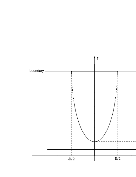
where the boundary condition is $\delta r(\pm D/2)=0$. Note that $r_{c}(x)$ solves $\delta S_{NG}=0$. For the sake of simplicity, $\delta r(x)$ is taken to be of arbitrarily long wavelength, i.e., $\frac{d\delta r(x)}{dx}\rightarrow 0$. In other words, the fluctuations at each string point are independent functions if one considers the long wavelength limit. The physical picture of the thermal fluctuations is shown in fig.3.

Figure 3: The effect of thermal fluctuations (dashed line) around the classical configuration (solid line). If $r_{*}$ is close enough to $r_{h}$, the fluctuations of very long wavelength may reach the horizon.

Then the string partition function that takes into account the fluctuations can be written as

$$Z_{str}\sim\int\mathcal{D}\delta r(x)e^{iS_{NG}(r_{c}(x)+\delta r(x))}.$$ (33)

By dividing the interval $-D/2<X<D/2$ into $2N$ points $x_{j}=j\Delta(x)$ with $j=-N,-N+1,...,N$ and $\Delta x\equiv D/(2N)$, one finds

$$Z_{str}\sim\lim_{N\to\infty}\int d[\delta r(x_{-N})]\cdots d[\delta r(x_{N})]exp[\frac{i\mathcal{T}\Delta x}{2\pi\alpha^{\prime}}\sum_{j}\sqrt{(r^{\prime}_{j})^{2}+a(r_{j})}],$$ (34)

where $r_{j}\equiv r(x_{j})$ and $r_{j}^{\prime}\equiv r^{\prime}(x_{j})$. The thermal fluctuations are more important around $x=0$, where $r=r_{*}$. Therefore, it is reasonable to expand $r_{c}(x_{j})$ around $x=0$, keeping only terms up to second order in $x_{j}$,

$$r_{c}(x_{j})\approx r_{*}+\frac{x_{j}^{2}}{2}r_{c}^{\prime\prime}(0),$$ (35)

where we have used the relation $r_{c}^{\prime}(0)=0$.

Also, the expansion for $a(r_{j})$, keeping only terms up to second order in $x_{j}^{m}\delta r_{n}$, reads

$$a(r_{j})\approx a_{*}+\delta ra^{\prime}_{*}+r_{c}^{\prime\prime}(0)a^{\prime}_{*}\frac{x_{j}^{2}}{2}+\frac{\delta r^{2}}{2}a_{*}^{\prime\prime},$$ (36)

where $a_{*}\equiv a(r_{*})$, $a^{\prime}_{*}\equiv a^{\prime}(r_{*})$, etc. Thus, the exponent in (34) can be approximated as

$$S_{j}^{NG}=\frac{\mathcal{T}\Delta x}{2\pi\alpha^{\prime}}\sqrt{C_{1}x_{j}^{2}+C_{2}},$$ (37)

with

$$C_{1}=\frac{r_{c}^{\prime\prime}(0)}{2}[2r_{c}^{\prime\prime}(0)+a_{*}^{\prime}],\qquad C_{2}=a_{*}+\delta ra_{*}^{\prime}+\frac{\delta r^{2}}{2}a^{\prime\prime}_{*}.$$ (38)

If the function in the square root of (37) is negative, $S_{j}^{NG}$ will contribute to an imaginary potential. The relevant region of the fluctuations is the one between $\delta r$ that yields a vanishing argument in the square root of (37). So, one can isolate the $j-$th contribution as

$$I_{j}\equiv\int_{\delta r_{jmin}}^{\delta r_{jmax}}d(\delta r_{j})exp[\frac{i\mathcal{T}\Delta x}{2\pi\alpha^{\prime}}\sqrt{C_{1}x_{j}^{2}+C_{2}}],$$ (39)

where $\delta r_{jmin}$ and $\delta r_{jmax}$ are the roots of $C_{1}x_{j}^{2}+C_{2}$ in $\delta r$.

The integral in (39) can be calculated by using the saddle point method for $\alpha^{\prime}<<1$ (the classical gravity approximation). The exponent has a stationary point when the function

$$D(\delta r_{j})\equiv C_{1}x_{j}^{2}+C_{2}(\delta r_{j}),$$ (40)

assumes an extremal value, and this happens for

$$\delta r=-\frac{a_{*}^{\prime}}{a_{*}^{\prime\prime}}.$$ (41)

It is required that the square root has an imaginary part, results in

$$D(\delta r_{j})<0\rightarrow-x_{c}<x_{j}<x_{c},$$ (42)

with

$$x_{c}=\sqrt{\frac{1}{C_{1}}(\frac{a_{*}^{\prime 2}}{2a_{*}^{\prime\prime}}-a_{*})}.$$ (43)

One takes $x_{c}=0$ if the square root in (43) is not real. With these conditions, one can approximate $D\delta(r)$ by $D(-\frac{a_{*}^{\prime}}{a_{*}^{\prime\prime}})$ in (39)

$$I_{j}\sim exp[\frac{i\mathcal{T}\Delta x}{2\pi\alpha^{\prime}}\sqrt{C_{1}x_{j}^{2}+a_{*}-\frac{a_{*}^{\prime 2}}{2a_{*}^{\prime\prime}}}].$$ (44)

As the total contribution to the imaginary part comes from $\Pi_{j}I_{j}$, one finds

$$ImV_{Q\bar{Q}}=-\frac{1}{2\pi\alpha^{\prime}}\int_{|x|<x_{c}}dx\sqrt{-x^{2}C_{1}-a_{*}+\frac{a_{*}^{\prime 2}}{2a_{*}^{\prime\prime}}}.$$ (45)

Integrating (45), one ends up with the imaginary potential for the transverse case as

$$ImV_{Q\bar{Q}}=-\frac{1}{2\sqrt{2}\alpha^{\prime}}(\frac{a_{*}^{\prime}}{2a_{*}^{\prime\prime}}-\frac{a_{*}}{a_{*}^{\prime}}).$$ (46)

Actually, there are several restrictions on Eq.(46) JN2 . First, the imaginary potential should be negative, so that

$$\frac{a_{*}^{\prime}}{2a_{*}^{\prime\prime}}-\frac{a_{*}}{a_{*}^{\prime}}>0,$$ (47)

with

$$a_{*}^{\prime}=e^{2P_{*}}(H_{*}^{\prime}+2H_{*}P_{*}^{\prime}),$$ (48)

$$a_{*}^{\prime\prime}=e^{2P_{*}}(H_{*}^{\prime\prime}+4H_{*}^{\prime}P_{*}^{\prime}+4H_{*}P_{*}^{\prime}P_{*}^{\prime}+2H_{*}P_{*}^{\prime\prime}),$$ (49)

which leads to

$$\varepsilon>\varepsilon_{min},$$ (50)

with $\varepsilon=1/(4r_{*}-3)$.

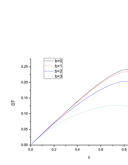
The second restriction is related to the maximum value of $DT_{max}$. To address this, we present $DT$ versus $\varepsilon$ for some choices of $b$ in the left panel of fig.4. One can see that in each plot there exists a maximum value of $DT_{max}$. As stated in JN2 , $DT_{max}$ indicates the limit of the saddle point approximation: to go to higher $DT$, there are other string configurations that may contribute to the calculation of the Wilson loops besides the semiclassical U-shaped string configuration DB , implying that one cannot calculate the imaginary potential in this case. On the other hand, we need to take $\varepsilon<\varepsilon_{max}$, where $\varepsilon_{max}$ is the maximum value of $\varepsilon$ for which the connected contribution is valid. Thus, the domain of applicability of Eq.(46) is $\varepsilon_{min}<\varepsilon<\varepsilon_{max}$.

Let us discuss results. First, we study the effect of the magnetic field on the inter-distance. From the left panel of fig.4, one can see clearly that increasing $b$ leads to decreasing $DT$. Namely, the inclusion of a magnetic field decreases the inter-distance, consistently with the findings of RRO .

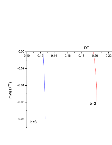
Next, we analyze the influence of a magnetic field on the imaginary potential. After considering $\varepsilon_{min}<\varepsilon<\varepsilon_{max}$, we compute the imaginary potential from (46), (48) and (49). In the right panel of fig.4, we plot Im$V/(\sqrt{\lambda}T)$ against $DT$ for $b=0,1,2,3$, corresponding to $\mathcal{B}/T^{2}\simeq 0,19,60,349$, respectively. From the figures one can see that for each plot the imaginary potential starts at a $DT_{min}$, corresponding to $\varepsilon_{min}$, and ends at a $DT_{max}$, corresponding to $\varepsilon_{max}$. And increasing $b$, the imaginary potential is generated for smaller distance. Namely, the magnetic field enhances the imaginary potential. As we know, the dissociation properties of quarkonia should be sensitive to the imaginary potential, and if the onset of the imaginary potential happens for smaller $DT$, the suppression will be stronger JN2 . On the other hand, a larger imaginary potential corresponds to smaller thermal width JN ; JN1 ; KB . Therefore, one concludes that the presence of the magnetic field tends to enhance the imaginary potential thus decreasing the thermal width. One step further, the magnetic field may make the suppression stronger. Intriguingly, it was argued RRO that the magnetic field has the effect of increasing the heavy quark potential thus decreasing the dissociation length, in agreement with the findings here.

Figure 4: Left: $DT$ versus $\varepsilon$ for $\theta=\pi/2$. From top to bottom $b=0,1,2,3$, respectively. Right: $ImV/(\sqrt{\lambda}T)$ versus $DT$ for $\theta=\pi/2$. From right to left $b=0,1,2,3$, respectively.

IV.2 Parallel to the magnetic field ($\theta=0$)

Next, we discuss the $Q\bar{Q}$ axis parallel to the magnetic field in the $z$ direction. The coordinates are parameterized as

$$t=\tau,\qquad x=0,\qquad y=0,\qquad z=\sigma,\qquad r=r(\sigma),$$ (51)

where the quark and anti-quark are located at $z=-\frac{D}{2}$ and $z=\frac{D}{2}$, respectively.

The next analysis is similar to the previous subsection, so we just show the final results. The inter-distance is

$$D=2\int_{r_{*}}^{\infty}dr\sqrt{\frac{A(r_{*})}{A^{2}(r)-A(r)A(r_{*})}}.$$ (52)

with

$$A(r)=H(r)e^{2K(r)},\qquad A(r_{*})=H(r_{*})e^{2K(r_{*})}.$$ (53)

The imaginary potential is

$$ImV_{Q\bar{Q}}=-\frac{1}{2\sqrt{2}\alpha^{\prime}}[\frac{A_{*}^{\prime}}{2A_{*}^{\prime\prime}}-\frac{A_{*}}{A_{*}^{\prime}}],$$ (54)

with

$$A_{*}^{\prime}=e^{2K_{*}}(H_{*}^{\prime}+2H_{*}K_{*}^{\prime}),$$ (55)

$$A_{*}^{\prime\prime}=e^{2K_{*}}(H_{*}^{\prime\prime}+4H_{*}^{\prime}K_{*}^{\prime}+4H_{*}K_{*}^{\prime}K_{*}^{\prime}+2H_{*}K_{*}^{\prime\prime}).$$ (56)

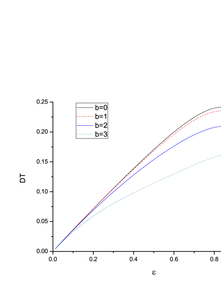
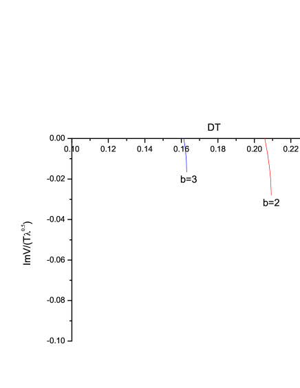
To study the effect of a magnetic field on the imaginary potential for the parallel case, we plot $DT$ versus $\varepsilon$ and Im$V/(\sqrt{\lambda}T)$ versus $DT$ in fig.5. From these figures, one can see that the behavior is very similar to the transverse case: the presence of the magnetic field decreases the inter-distance and enhances the imaginary potential. In addition, by comparing fig.4 and fig.5, one can see that the magnetic field has a stronger effect for the transverse case rather than parallel. Interestingly, a similar observation has been found in RRO which argues that the magnetic field has stronger effect on the heavy quark potential for the perpendicular configuration.

Figure 5: Left: $DT$ versus $\varepsilon$ for $\theta=0$. From top to bottom $b=0,1,2,3$, respectively. Right: $ImV/(\sqrt{\lambda}T)$ versus $DT$ for $\theta=0$. From right to left $b=0,1,2,3$, respectively.

V conclusion and discussion

In this paper, we studied the effect of a constant magnetic on the imaginary potential of quarkonia in strongly-coupled $\mathcal{N}=4$ SYM plasma. We considered the pair axis to be aligned perpendicularly and parallel to the magnetic field, in turn. In both cases, it is shown that the inclusion of the magnetic field enhances the imaginary potential thus decreasing the the thermal width. Also, the magnetic field has a stronger effect for the perpendicular case rather than parallel.

However, it should be noted that the magnetized plasma considered here is different from the real QGP, mainly due to the lack of a dynamical breaking of conformal symmetry. It would be interesting to investigate modifications of the holographic setup addressed here and consider the systems that are not conformal. We leave this for further study.

VI Acknowledgments

The authors would like to thank the anonymous referee for his/her valuable comments and helpful advice. This work is partly supported by the Ministry of Science and Technology of China (MSTC) under the 973 Project No. 2015CB856904(4). Z-q Zhang is supported by NSFC under Grant No. 11705166. D-f. Hou is partly supported by the NSFC under Grants Nos. 11735007, 11521064.

References

- (1) J. Adams et al. [STAR Collaboration], Nucl. Phys. A 757, 102 (2005).
- (2) K. Adcox et al. [PHENIX Collaboration], Nucl. Phys. A 757, 184 (2005).
- (3) E. V. Shuryak, Nucl. Phys. A 750, 64 (2005).
- (4) T. Matsui, H. Satz, Phys. Lett. B 178, 416 (1986).
- (5) M. Laine, O.Philipsen, P. Romatschke and M. Tassler, JHEP 03 (2007) 054
- (6) A. Beraudo, J.-P. Blaizot, and C. Ratti, Nucl. Phys. A806, 312 (2008).
- (7) N. Brambilla, J. Ghiglieri, A. Vairo, and P. Petreczky, Phys. Rev. D 78, 014017 (2008).
- (8) M. A. Escobedo, J. Phys. Conf. Ser. 503 (2014) 012026.
- (9) N. Brambilla, M.A. Escobedo, J. Ghiglieri, J. Soto and A. Vairo, JHEP 09 (2007) 038
- (10) A. Dumitru, Y. Guo, and M. Strickland, Phys.Rev. D79 (2009) 114003.
- (11) M. Margotta, K. McCarty, C. McGahan, M. Strickland, and D. Y. Elorriaga, Phys.Rev. D 83 (2011) 105019.
- (12) V. Chandra and V. Ravishankar, Nucl. Phys. A 848 (2010) 330.
- (13) J. M. Maldacena, Adv. Theor. Math. Phys. 2, 231 (1998).
- (14) S. S. Gubser, I. R. Klebanov and A. M. Polyakov, Phys. Lett. B428, 105 (1998).
- (15) O. Aharony, S. S. Gubser, J. Maldacena, H. Ooguri and Y. Oz, Phys. Rept. 323, 183 (2000).
- (16) J. C. Solana, H. Liu, D. Mateos, K. Rajagopal, and U. A. Wiedemann, arXiv:1101.0618.
- (17) J. Noronha, A. Dumitru, Phys. Rev. Lett. 103 (2009) 152304.
- (18) S. I. Finazzo, J. Noronha, JHEP 11 (2013) 042.
- (19) K. B. Fadafan, D. Giataganas and H. Soltanpanahi, JHEP 11 (2013) 107
- (20) S. I. Finazzo, J. Noronha, JHEP 01 (2015) 051.
- (21) M. Ali-Akbari, D. Giataganas and Z. Rezaei, Phys. Rev. D 90 (2014) 086001.
- (22) K. B. Fadafan, S. K. Tabatabaei, J. Phys. G: Nucl. Part. Phys. 43 095001 (2016).
- (23) Z. q. Zhang, D.f. Hou, and G. Chen, Phys. Lett. B 768, 180 (2017).
- (24) N. F. Braga and L. F. Ferreira, Phys. Rev. D 94, 094019 (2016).
- (25) J. Sadeghi and S. Tahery, JHEP 06 (2015) 204.
- (26) J. L. Albacete, Y. V. Kovchegov, A. Taliotis, Phys. Rev. D 78 (2008) 115007.
- (27) T. Hayata, K. Nawa, T. Hatsuda, Phys. Rev. D 87 (2013) 101901.
- (28) E. D. Hoker and P. Kraus, JHEP 10 (2009) 088.
- (29) K. A. Mamo, JHEP 08 (2013) 083.
- (30) R. Critelli, S. I. Finazzo, M. Zaniboni, and J. Noronha, Phys. Rev. D 90, 066006 (2014).
- (31) R. Rougemont, R. Critelli and J. Noronha, Phys. Rev. D 91, 066001 (2015).
- (32) K. A. Mamo, Phys. Rev. D 94, 041901(R) (2016).
- (33) S. Li, K. A. Mamo and H.U.Yee, Phys. Rev. D 94, 085016 (2016).
- (34) J. M. Maldacena, Phys. Rev. Lett. 80, 4859 (1998).
- (35) A. Brandhuber, N. Itzhaki, J. Sonnenschein and S. Yankielowicz, Phys. Lett. B 434, 36 (1998).
- (36) S. -J. Rey, S. Theisen and J. -T. Yee, Nucl. Phys. B 527, 171 (1998).
- (37) D. Bak, A. Karch, L. G. Yaffe, JHEP 0708 (2007) 049.