Complexity of the laminar-turbulent boundary in pipe flow
Abstract
Over the past decade, the edge of chaos has proven to be a fruitful starting point for investigations of shear flows when the laminar base flow is linearly stable. Numerous computational studies of shear flows demonstrated the existence of states that separate laminar and turbulent regions of the state space. In addition, some studies determined invariant solutions that reside on this edge. In this paper, we study the unstable manifold of one such solution with the aid of continuous symmetry-reduction, which we formulate here for the first time for the simultaneous quotiening of axial and azimuthal symmetries. Upon our investigation of the unstable manifold, we discover a previously unknown traveling wave solution on the laminar-turbulent boundary with a relatively complex structure. By means of low-dimensional projections, we visualize different dynamical paths that connect these solutions to the turbulence. Our numerical experiments demonstrate that the laminar-turbulent boundary exhibits qualitatively different regions whose properties are influenced by the nearby invariant solutions.
pacs:
02.20.-a, 05.45.-a, 05.45.Jn, 47.27.edI Introduction
Pipe flow is the most prominent member of a class of canonical shear flows where transition to turbulence occurs despite the linear stability of the laminar state Meseguer and Trefethen (2003). In the past two decades this problem enjoyed several major developments. The discovery of nonlinear traveling wave solutions Faisst and Eckhardt (2003); Pringle and Kerswell (2007); Pringle et al. (2009) and studies Schneider et al. (2007); Duguet et al. (2008); Mellibovsky et al. (2009) of the laminar-turbulent boundary began to elucidate the state space of the system using insights from dynamical systems theory.
In the dynamical systems approach to turbulence, fluid motion is envisioned as a trajectory in an infinite-dimensional state space (Hopf, 1948). For the case of shear flows with linearly stable laminar solutions, this state space accommodates a stable equilibrium point corresponding to the laminar solution and a chaotic set (an attractor or repellor) that is turbulence. Once this viewpoint is established, a natural question to ask is what separates these two distinct regions in the state space. In a small computational cell of channel flow, Itano and Toh Itano and Toh (2001) were first to study solutions that neither laminarize nor become turbulent using a shooting method and they discovered such trajectories tend towards a traveling wave solution. Following studies of shear flows in similar computational domains found periodic-like (Toh and Itano, 2003), equilibrium (Schneider et al., 2008), as well as seemingly chaotic (Schneider et al., 2007) solutions using similar shooting methods. These findings suggested the following picture of the state space of shear flows: The basin boundary between laminar and turbulent solutions is the stable manifold of an invariant set, whose unstable manifold on one side connects to the laminar solution and on the other side to the turbulent part of the state space. Schneider et al. Schneider et al. (2007) named this invariant set the “edge state”.
Schneider et al. Schneider et al. (2007) found in a short axially-periodic computational domain of pipe flow that the edge state exhibits chaotic motion, with flow structures much simpler than those of turbulence: a slow streak in the center surrounded by two fast streaks with chaotically moving streamwise vortices in between. A similar investigation in a long computational domain of pipe flow Mellibovsky et al. (2009) yielded stream-wise localized edge states with chaotic dynamics, whose flow fields at the core of the localized structure resembled those computed in the short computational domain.
Typically when flows are not simplified by additional symmetries the edge state tends to be chaotic as is the case for plane Couette Schneider et al. (2010), channel Zammert and Eckhardt (2014), and asymptotic suction boundary layer Khapko et al. (2016) flows. In this seemingly generic case, the definition of the edge state is less clear than when it is formed by an exact invariant solution such as an (relative) equilibrium or a (relative) periodic orbit. In contrast to the invariant solutions, it is not straightforward to define and compute the stable/unstable manifolds of chaotic solutions, hence their theoretical study is much more challenging.
One way of systematically investigating chaotic edge states is studying the unstable invariant solutions that are contained within, since the geometry of chaotic sets are influenced by the invariant solutions that are embedded in them Cvitanović et al. (2015). This strategy was adopted by Duguet et al. Duguet et al. (2008), who found for the case of pipe flow in an approximately 5-diameters long, axially periodic computational domain at (Re based on bulk velocity and pipe diameter) that the chaotic edge state evolves around the “asymmetric” traveling wave solution found by Pringle and Kerswell Pringle and Kerswell (2007). In addition, they found a rotating traveling wave that had flow structures very similar to those of the asymmetric wave, but differently it rotated in the azimuthal direction in addition to drifting downstream.
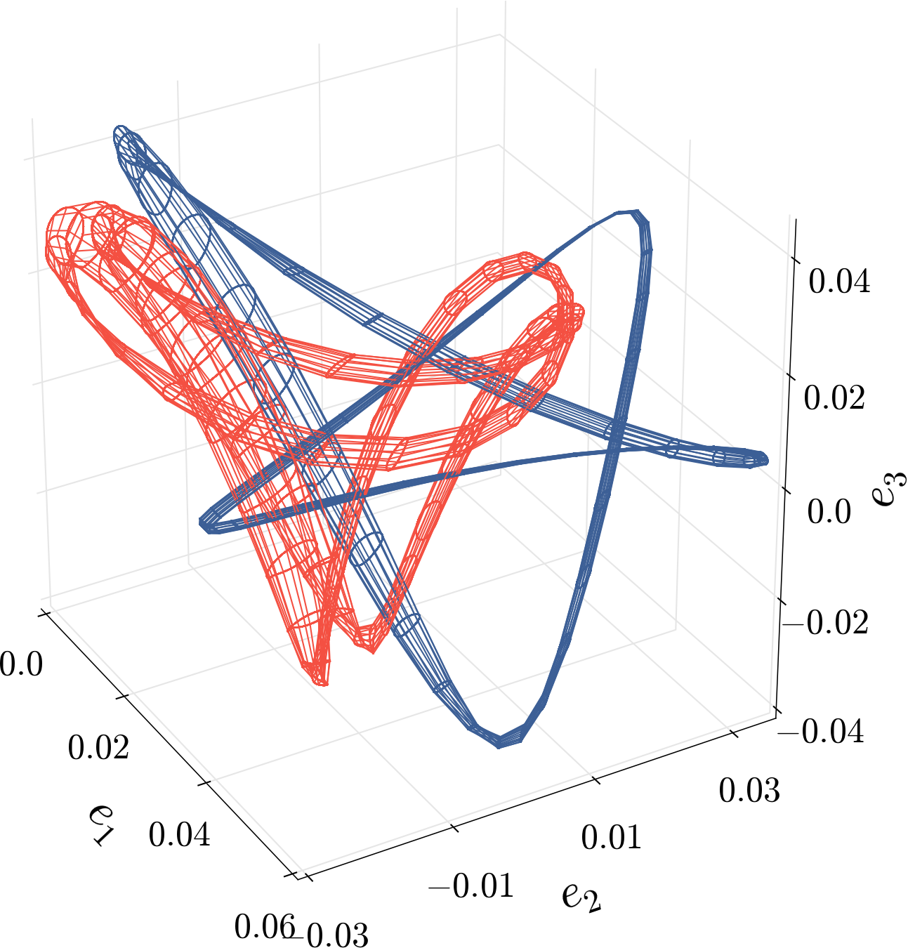
Canonical shear flows (pipe, plane Couette, and plane Poiseuille) are symmetric under continuous translations in streamwise and spanwise (or azimuthal, in the case of pipe flow) directions. This implies that every generic (non-symmetric) solution of these systems have infinitely many copies that can be generated by symmetry transformations. We visualized this degeneracy on figure 1 for two traveling wave solutions we study in this article. Due to this multiplicity, something as simple as measuring the distance between two solutions becomes a daunting task. As a result, a common practice in dynamical systems approach to turbulence literature is to use quantities averaged over computational domains, such as energy input, dissipation, or pressure gradient, as indicators of “closeness” in the state space Kawahara and Kida (2001); Viswanath (2007); Ritter et al. (2016); Khapko et al. (2016). While observing such quantities can be used for deciding if two solutions are far from each other, they cannot be used to conclusively decide if two solutions are close in the state space: Two solutions that have similar rates of energy input, dissipation, and pressure drop might have completely different flow structures. In this paper, this problem is addressed by symmetry reduction, for the first time in both axial and azimuthal directions of pipe flow. In the symmetry-reduced state space, the tori, such as those visualized on figure 1, are represented by single points, which simplifies the analysis substantially. As we will explain later in the article, our approach to this problem is generic and adaptable to other canonical shear flow geometries in a straightforward fashion.
For the application of our methods, we chose to revisit the laminar-turbulent boundary in a short ( diameters) pipe flow at . To this end, we visualize numerical approximations to the unstable manifold of the asymmetric traveling wave that reside in the laminar-turbulent boundary on local projections akin to those pioneered by Gibson et al. Gibson et al. (2008). We demonstrate that some parts of this unstable manifold that belong to the laminar-turbulent boundary exhibit dynamics qualitatively different from those previously attributed to the edge state in this setting. Upon further investigation, we discover that this region is in the vicinity of a previously unknown traveling wave solution with four high-speed streamwise streaks. This new traveling wave appears to belong to a higher-energy region in the edge state; closer to the turbulent part of the state space. We study the unstable manifold of the new traveling wave and demonstrate its different connections to the turbulence. Finally, we present the results of numerical experiments, which demonstrate that the trajectories on laminar-turbulent boundary of pipe flow transiently approach to the traveling waves that reside in the edge.
The rest of the paper is organized as follows. In the next section, we overview our methods, particularly in section II.4, we present the generalization of the first Fourier mode slice (Budanur and Hof, 2017) for simultaneous reduction of continuous symmetries in axial and azimuthal directions. We present our results in section III, followed by the discussion in section IV.
II Methods
II.1 Numerical set-up
Numerical integration of the Navier–Stokes equations
| (1) |
are performed using Openpipeflow (Willis, 2017). The velocity field denotes the deviations from the base (Hagen-Poiseuille) solution . Lengths and velocities are nondimensionalized by the pipe diameter , and the mean axial speed . Boundary conditions are no-slip and impermeable on pipe walls ; periodic in axial and azimuthal directions . The velocity field satisfies the incompressibility condition and is a feedback term, adjusted in order to ensure a constant-flux equal to that of the laminar solution at a given Re. For all results of this paper, ; the pipe length is set to ; flow fields are discretized using finite-difference points in radial direction and Fourier series truncated at respectively in axial and azimuthal directions. Nonlinear terms are evaluated in the physical space on grid points following the -rule for dealiasing in Fourier-expanded directions. This truncation yields more than numerical degrees of freedom, which is significantly higher than the typical resolutions used in similar computational studies Schneider et al. (2007); Wedin and Kerswell (2004). Our choice yields at least orders of magnitude drop in the spectral coefficients of the turbulent solutions at . While the solutions in the edge state generally require much less degrees of freedom to be resolved, we made this “conservative” choice since we investigate different regions of the edge state and we did not know a priori the maximum resolution requirement.
II.2 Symmetries
In this section, we review the symmetries of pipe flow and their representations in terms of their actions on the velocity field. For more detailed discussions of the symmetries and the invariant subspaces of pipe flow, we refer the reader to refs. Budanur et al. (2017); Willis et al. (2013). Pipe flow is equivariant under the axial translations , the azimuthal rotations , and the reflection ; whose actions on the axial , radial , and azimuthal components of the velocity field are given by
| (2) | |||||
| (3) | |||||
| (4) |
Therefore, the symmetry group of pipe flow is the direct product of and , i.e.
| (5) |
II.3 State space notation
Since we are going to use dynamical systems tools, it is handy to introduce a state space notation for use in the rest of the paper. Let be a vector that contains all numerical degrees of freedom of a three-dimensional velocity field at an initial time . Then, the Navier–Stokes equations (1) along with the incompressibility and the boundary conditions imply a finite-time flow
| (8) |
where corresponds to the velocity field at time . Assuming that the flow (8) is smooth, we can also represent the system as a high-dimensional ordinary differential equation
| (9) |
Actions of group elements on a state space vector should be thought as actions on the corresponding velocity fields as in (2–4). In other words, if corresponds to velocity field then corresponds to the transformed velocity field . Similarly, group tangents correspond to velocity fields , where acts as in (7). In the state space, equivariance under implies that state space velocity and finite-time flow commutes with , i.e.
| (10) |
Let and correspond to velocity fields and respectively, we define the inner product
| (11) |
where the integral is carried over the pipe volume. Thus, gives the kinetic energy of the velocity fluctuations; hence this choice of norm is usually referred to as the “energy norm”.
II.4 Continuous symmetry reduction
We define the group orbit of a state space point as all points reachable from by symmetry transformations, i.e.
| (12) |
If is not invariant under any symmetries of the system, its group orbit (12) defines two distinct two-tori that are related to each other by the reflection since we have two compact continuous symmetry directions (5). All state space points on a group orbit have the same physical properties, such as kinetic energy, dissipation, or wall-friction since these quantities are invariants of symmetry transformations. In addition, the dynamics of each point on a group orbit can be obtained from the dynamics of a single point following the definition (10) of equivariance. In other words, the state space of pipe flow exhibits a lot of redundancy since a generic point have infinitely many symmetry copies. Moreover, the presence of continuous symmetries renders the study of state space extremely hard: in the presence of pipe flow’s symmetries, measuring the distance between two generic state space points becomes the question of the minimum distance between tori, whose computational cost can easily become prohibitive if it is to be carried out repeatedly. Continuous symmetry reduction, which we introduce next, is a coordinate transformation such that state space points that are related by a continuous symmetries are represented by a single point in the reduced state space.
We begin by reducing the streamwise translation symmetry following Budanur and Hof (2017) exactly: We define a “slice template” with a corresponding three-dimensional velocity field, whose each component is defined as
| (13) |
where is the Bessel function of the first kind, which vanishes at the pipe wall, i.e. . Then the translation symmetry-reduced coordinates are given by
| (14) | |||||
| (15) |
The transformation (14) exists as long as the phase (15) does. Note that is the polar angle when the state is projected onto the plane spanned by .
Extension of (14) for the azimuthal symmetry reduction is straightforward with a second slice template corresponding to the velocity field with components
| (16) |
Then the symmetry-reducing coordinate transformation becomes
| (17) | |||||
| (18) |
Similar to (14) and (15), the transformation (17) exists as long as the phase (18) does. Our choice of the order at which the continuous symmetries are reduced is merely a convention since the inner products in (15) and (18) remain unchanged respectively under transformations (17) and (14). This is a result of our particular choice of the slice templates (13) and (16), which respectively do not depend on and and the fact that the axial translation and the azimuthal rotation symmetries commute. For a general symmetry group with non-commuting elements, a more careful treatment would have been required.
The slice templates (13) and (16) need not be valid (smooth, divergence free) pipe flow velocity fields. The only requirement on the slice templates and is that the projections of the 2-torus onto the - and -planes both must be circles for a generic state . Cosine-dependence of (13) and (16) on the respective symmetry directions provides this as long as the projection is nonzero. We determine the rest of the slice templates by experimentation in order to reduce the probability of having a vanishing projection: We decided to use all three velocity components for the template-fields in order to receive contributions from all directions. The radial-dependence on , on the other hand, is an arbitrary and it is conceivable that there could be other equally valid choices. As we will further argue after introducing the slice phase velocities (25), our experience with the slice templates (13) and (16) has been that the symmetry-reduction procedure that we described yields no discontinuities when applied to the generic turbulent trajectories.
Budanur et al. Budanur et al. (2015a) showed for a one-dimensional PDE with symmetry that polar coordinate transformations similar to (14) and (17) can be reformulated as a “slice hyperplane”. A slice hyperplane is a set of points perpendicular to the group orbit of a slice template and is transversally intersected by the group orbits of the state space points in a closed neighborhood of the template. While a general slice has a finite region of applicability, if the template is chosen such that its dependence on the symmetry coordinate depends only on the first Fourier mode, then the slice works for a semi-infinite domain (half-hyperplane) that covers all state space of interest, with a regularizable singularity in time. This method is named “first Fourier mode slice” in (Budanur et al., 2015a) and we refer the reader to (Budanur et al., 2015b) for a pedagogical introduction to it.
Reduced coordinates (14) satisfy the half-hyperplane equation
| (19) |
where is the group tangent of a state space point and . Similarly, we can express the consequent transformation (17) as another half-hyperplane in the streamwise symmetry-reduced state space as
| (20) |
where similarly, and .
The main advantage of the reformulations (19) and (20) is that from this perspective one is able to derive projection operators for transforming the tangent space of to the slice. Let be a small perturbation to in the full state space, and be the slice phase that brings to slice as , then the small perturbation can be brought to the slice by the projection
| (21) |
Similarly, is transformed to the second slice (20) as
| (22) |
where is the slice-fixing phase (18), i.e. . For the derivation of these projection operators, we refer to the appendix of (Budanur and Hof, 2017).
We are going to finish this section by explaining possible short-comings of the presented symmetry-reduction scheme: With the aid of the projections (21) and (22), it is straightforward to express state space velocity in the reduced state space. Substituting with in (21) we obtain
| (23) |
where we used the first equivariance property in (10) and defined the stream-wise symmetry-reduced state space velocity as . The fully symmetry-reduced state space velocity can be similarly written as
| (24) |
It is instructive to have a close look at (23): The reduced state space velocity is generated from full state space velocity by subtracting the component in the direction of the group tangent with a pre-factor proportional to ’s projection onto the slice tangent. The second thing to recognize in (23) is the fact that appears in the denominator, hence if this inner product vanishes, the reduced state space velocity field diverges. For a general slice, this condition sets the border in which the slice may apply Froehlich and Cvitanović (2012); Cvitanović et al. (2012); in our particular case of the first Fourier mode slice, this condition is equivalent to the existence of the phase (15). It can be shown Rowley and Marsden (2000) that the multipliers of group tangents in (23) and (24) correspond to the time derivatives of the parameters of group actions that bring trajectories to the slice, i.e.
| (25) |
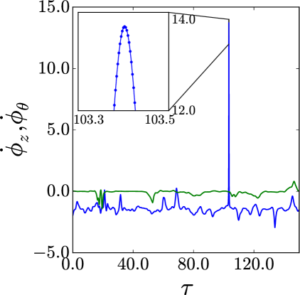
Hence, these are appropriate quantities for checking whether or not the sliced dynamics is within its borders. Our experience with the first Fourier mode slices has been such that these quantities do not diverge for generic trajectories, although they may have “fast” episodes. We illustrate this for a typical turbulent trajectory in figure 2. Fast fluctuations that are caused by such episodes can be handled by rescaling the time-step of the numerical simulation or the problem can be explicitly reformulated using a “slice time” Budanur et al. (2015a). In this study, we found a fixed time-step to be sufficient to resolve the changes in slice phases, without resorting to an adaptive time-stepping scheme.
III Traveling waves on the laminar-turbulent boundary
Other than the laminar equilibrium, all invariant solutions such as traveling waves, rotating waves, relative periodic orbits, and possibly higher-dimensional invariant tori, of pipe flow drift downstream. A traveling wave is the simplest among those, which satisfies
| (26) |
namely, its sole dynamics is a drift in the axial direction with constant phase speed . Linear stability of this solution is described by the following eigenvalue problem Chossat and Lauterbach (2000); Cvitanović et al. (2015)
| (27) |
where and are the linear stability eigenvalues and eigenvectors respectively. Since the state space is formally infinite-dimensional, each traveling wave has infinitely many stability eigenvalues and eigenvectors. In practice, we solve (27) by Arnoldi iteration and approximate the finite-dimensional leading (most unstable) part of the tangent space.
Traveling waves become equilibria when the axial translation symmetry is reduced, say by the first Fourier mode slice method of (14). The translation symmetry-reduced state space still exhibits the and it follows from the normal form analysis that all equilibria of an -equivariant system belong to invariant subspaces of reflection symmetry or its conjugates Armbruster et al. (1988). Coming back to full state space, this implies that all traveling waves of pipe flow must be invariant under the reflection or a related symmetry. In particular, the solutions we are going to investigate in what follows are invariant under so-called shift-and-reflect symmetry
| (28) |
In the shift-and-reflect subspace, continuous rotation symmetry (3) of the pipe flow is broken and only the discrete rotation by is allowed (Budanur et al., 2017). Thus, the symmetry group of shift-and-reflect subspace is
| (29) |
Note that by definition, reflection symmetry is equivalent to an axial-translation by .
III.1 Unstable manifold of S1
Numerical (Duguet et al., 2008) and experimental (de Lozar et al., 2012) (combined with numerical work) evidence strongly suggests that the edge state of axially periodic pipe flow that is not long enough to exhibit streamwise localization is organized around the asymmetric traveling wave solution found in Pringle and Kerswell (2007). Following Pringle et al. (2009), we are going to refer to this solution as S1. This naming refers to solution’s symmetries: stands for ‘shift-and-reflect’ (28) invariance and is the fundamental azimuthal wave number. appears at a low-Re through a symmetry-breaking bifurcation of a -symmetric solution, which itself is born out of a saddle-node bifurcation at even lower Re Pringle and Kerswell (2007). For the parameters studied here () S1 and its two purely real unstable eigenvectors with corresponding eigenvalues are visualized in figure 3. On figure 3 (a) and throughout the three-dimensional visualizations of this paper, streamwise velocity isosurfaces are chosen as of their maximum/minimum values for velocity fluctuations. Similarly, vorticity isosurface levels are chosen at of their respective maxima and minima. Numerical values of velocity/vorticity isosurfaces are given in the figure caption. For the two-dimensional cross-sectional visualizations of shift-and-reflect-symmetric states, we chose to average quantities over the first half pipe-length since the second half is simply the reflection of the first.
(a) 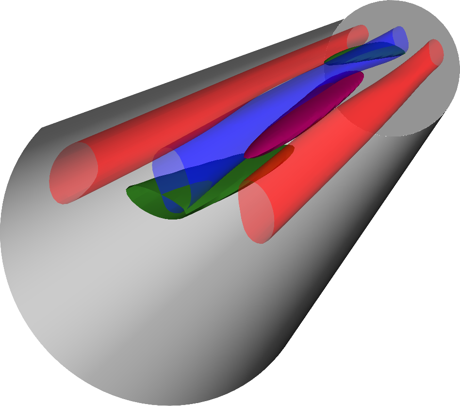 (b)
(b) 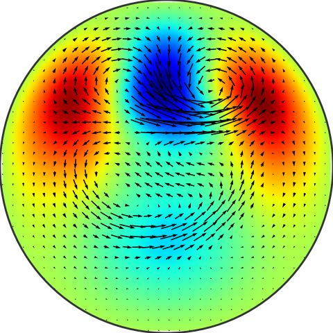
(c) 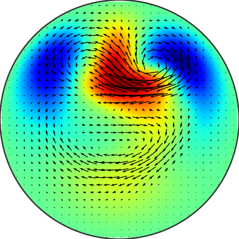 (d)
(d) 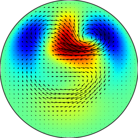 (e)
(e) 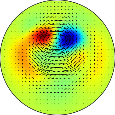 (f)
(f) 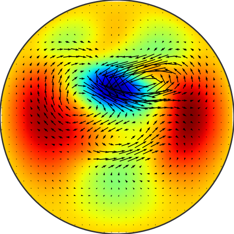
In figure 3, besides the eigenvectors (figure 3 c and e), which are computed in the full state space, we also show (figure 3 d and f), which are obtained by the projection (21). With these visualizations, we would like to emphasize that the symmetry-reduced eigenvector might be quite different from the one that is computed in the full state space as it is the case for (figure 3 e) and (figure 3 f). Moreover, it should be understood that the unstable manifold of S1 in the full state space is three-dimensional whose linear part is contained within the tangent space spanned by , , and the marginal direction with the eigenvalue . Note that the projection (21) subtracts components in this direction and its action on yields a zero vector. In other words, the marginal stability direction, which corresponds to axial drift of the traveling wave, is eliminated by slicing. Thus within the slice, S1 has a two-dimensional unstable manifold, whose linear part is contained in the -plane.
Duguet et al. Duguet et al. (2008) studied the evolution of perturbations along the unstable directions of S1. After confirming that the perturbations in direction either laminarizes or develops into turbulence, they focused on the perturbations on plane that neither laminarize nor become turbulent. Running Newton searches near-recurrences of these trajectories, they found a rotated versions of S1 and conjectured that S1’s unstable manifold contains a “relative”-heteroclinic connection to its rotation by approximately . This cannot be true since the unstable eigenvectors and are also shift-and-reflect symmetric, hence the associated unstable manifold lies in the shift-and-reflect invariant subspace, which only allows for azimuthal rotations by . We are guessing that Duguet et al.’s conjecture was a result of a numerical error build up due to not restricting dynamics into the shift-and-reflect invariant subspace. Our first calculation in this paper will be very similar to theirs, with the symmetry-restriction requirement taken into account. In addition, we are going to carry out our computation in the translation symmetry-reduced state space (14), which will allow us to visualize the unstable manifold.
As a first approximation to S1’s unstable manifold, we start trajectories with the initial conditions
| (30) |
where is the symmetry-reduced state space point corresponding to S1, and are S1’s leading linear stability eigenvectors projected onto the slice as described in (21), and is a small constant. (30) defines an ellipse on the -hyperplane, parametrized by and the scaling of perturbations by corresponding eigenvalues lets trajectories expand initially at similar rates (Krauskopf et al., 2005). This is illustrated on the inset of figure 4 (a) where for is shown for equally spaced trajectories in as projections onto the local bases formed by orthogonalizing , i.e.
| (31) |
In (31), subscript indicates that are orthonormalized via the Gram-Schmidt procedure; i.e. is formed by subtracting ’s projection onto the direction and normalization. The inset of figure 4 (a) illustrates that these bases capture local dynamics very well. In particular, note that the trajectories starting from the initial conditions (30) with are initially straight as they correspond to the perturbations in the symmetry-reduced eigenvector directions; whereas the rest appear bend since the two unstable directions expand at different rates. Outer panel of figure 4 shows these trajectories for longer times, until they either become turbulent or laminarize. The trajectories that become turbulent or relaminarize are respectively colored pink and gray. While the projections are locally reliable, they fail to fully capture the dynamics away from S1 since the trajectories seem to fold onto themselves. In order to illustrate the qualitative features of the transition, we marked instances on at and visualized the corresponding three-dimensional flow structures on figure 4 (b, c, d). Note that the structures on figure 4 (b) are quite similar to those of S1, while the isosurface levels are set to higher values. This illustrates the first part of the transition: As the trajectory moves from S1 towards turbulence, streaks and vortices are amplified while their overall shape is more or less unchanged. As can be seen on figure 4 (c), this initial amplification is followed by the breakdown of streaks, and eventual turbulence (d) no longer exhibits structures that are coherent throughout the computational domain.
(a) 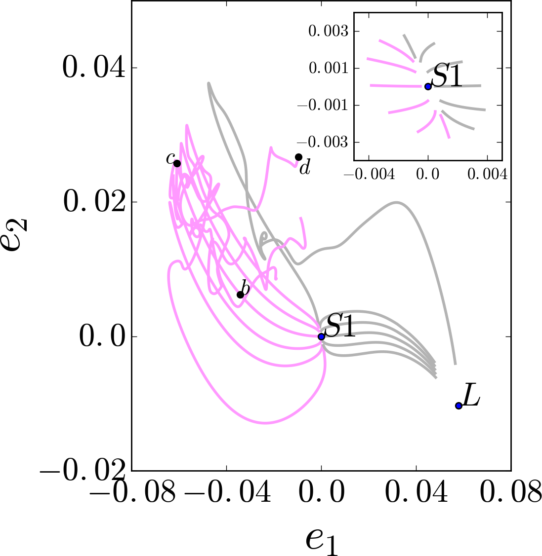
(b) 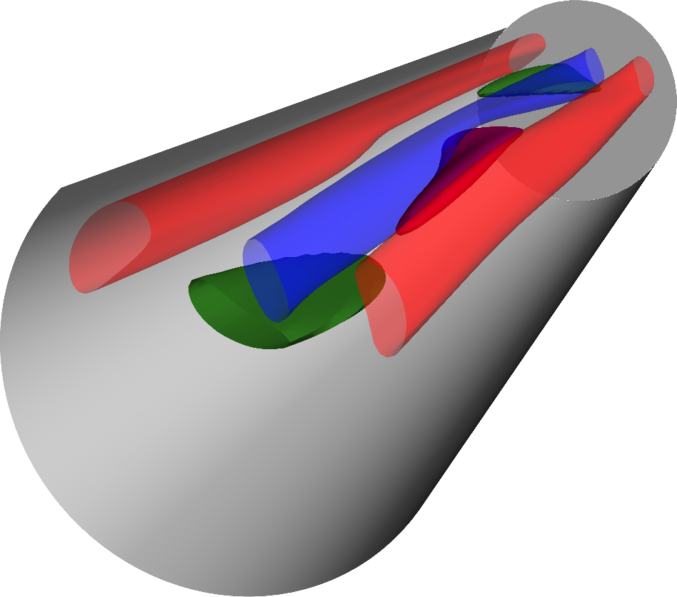
(c) 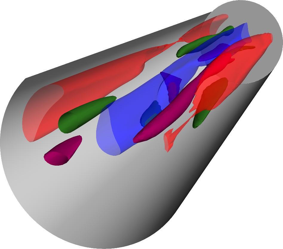
(d) 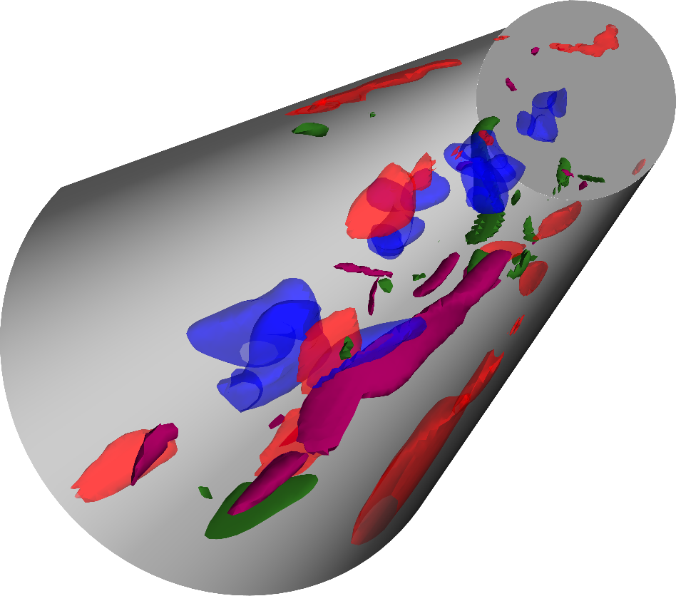
The -trajectory approximation to the -dimensional unstable manifold is initially successful and illustrates the general features of the unstable manifold, such as relaminarization and transition to turbulence. It is clear from figure 4(a) that this approximation very quickly fails to cover the extend of the manifold that stays in the laminar-turbulent boundary. In order to uncover details of this part, we bisected between trajectories that transition to turbulence or relaminarize by changing in (30) until reaching the limit of numerical precision, as done in Duguet et al. (2008). Differently, however, we enforced shift-and-reflect invariance in the time-stepping, in order to avoid numerical errors that could take trajectories outside the invariant subspace. In order to improve visibility, we visualized the unstable manifold approximated this way in three dimensions, using the least contracting stability eigenvector (symmetry reduced and orthonormalized) in addition to the leading-two (31) as the third basis. The unstable manifold visualized this way is shown in figure 5(a), where we coloured trajectories that eventually laminarize gray, and those that transition to turbulence pink. Additionally, we plotted the last four trajectories in the bisection procedure thicker than the rest, using colors red, blue, green, and black. For comparison, time series of the kinetic energy for these four trajectories is shown in figure 5(b), where we see that the trajectories stay on the ‘edge’ longer than time units.
(a) 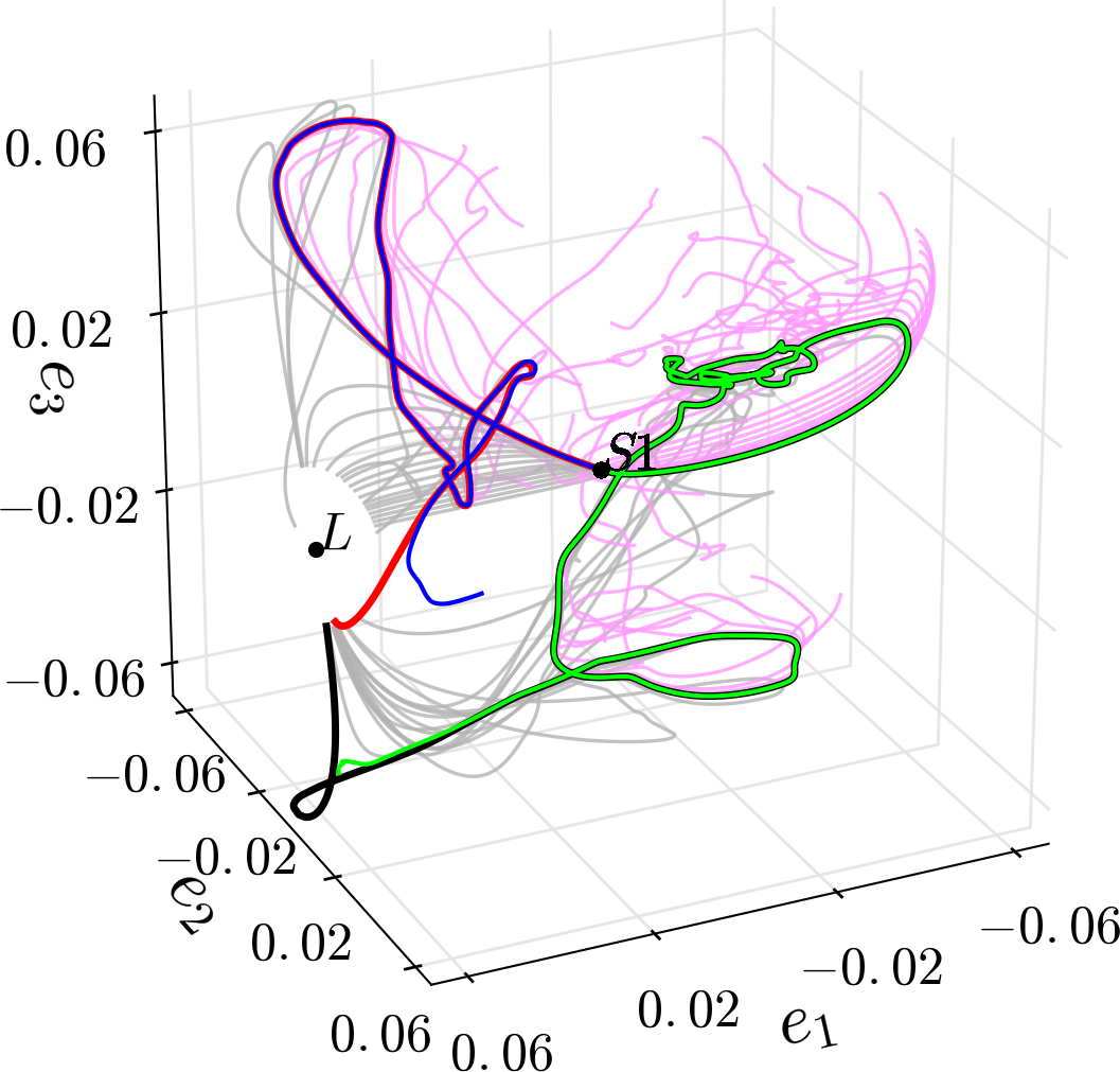 (b)
(b) 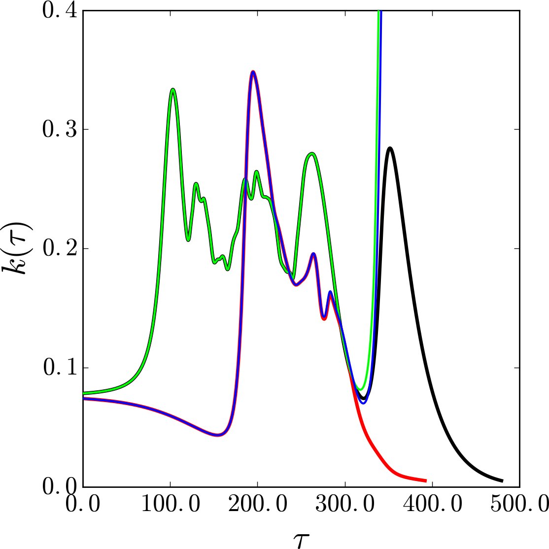
Upon our investigation of the trajectories that stay on the edge for the longest times, we observed episodes where state space trajectories slow down, which might indicate visits to the neighborhoods of other traveling waves. In order to quantify this, we measured the “self-recurrence”, which we defined as the norm of the difference between the symmetry-reduced states at time and on the same trajectory. Note that in the symmetry-reduced state space, the traveling waves are equilibria thus no extra care for the translation symmetry is necessary. Figure 6 shows the self-recurrence (a) over the trajectory which is shown blue on figure 5 and flow structures at different times on this trajectory (b-e).
(a) 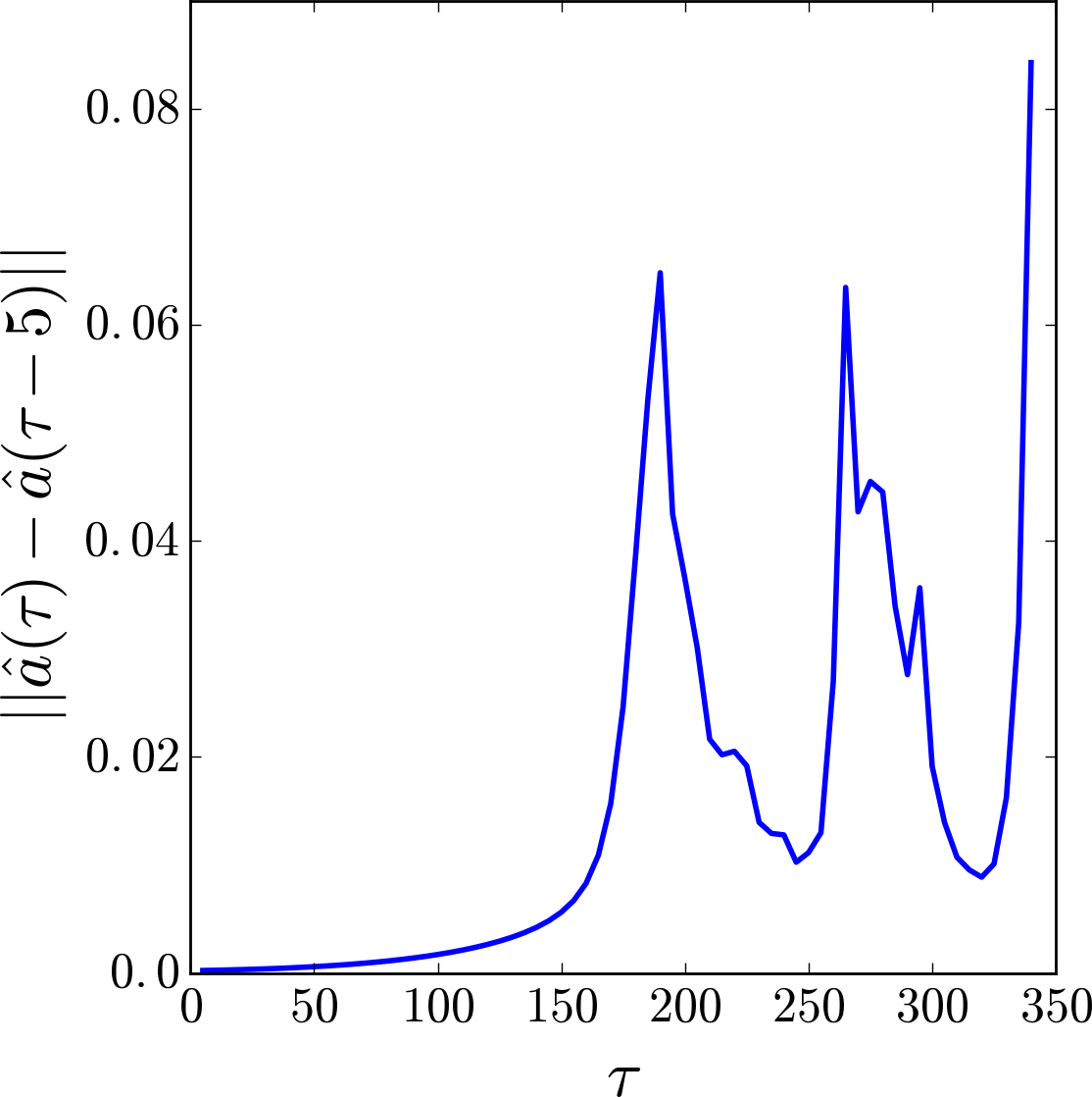
(b)  (c)
(c) 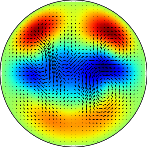
(d) 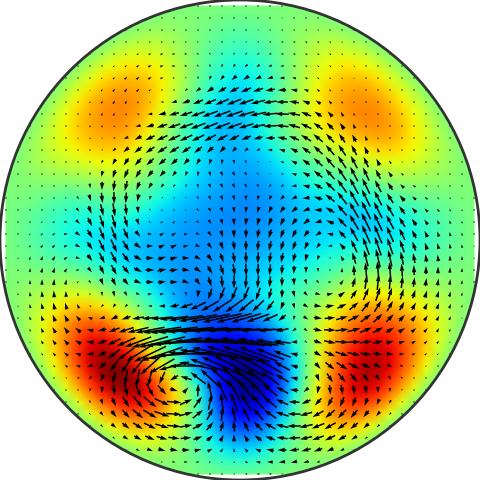 (e)
(e) 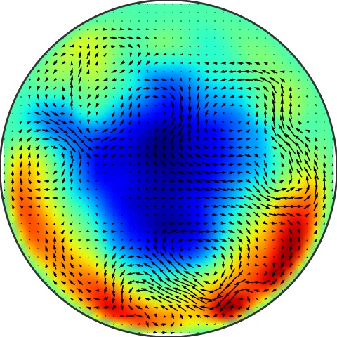
As the trajectory evolves on the edge, it visits states with qualitatively different features: At the first minimum (figure 6 (c)) of the self-recurrence function, new fast streaks begin to form on the down-side of the pipe cross-section and at the second minimum (figure 6 (d)) initial fast streaks begin to disappear. Eventual transition to turbulence (figure 5 (e)) has quantitative features similar to those illustrated in figure 4: streaks amplify, spread, and break into smaller scale structures on the opposite side of the pipe. Newton-Krylov-hookstep searches starting from initial conditions visualized on figure 6 (c) and (d) converged to traveling wave solutions: Starting from the latter, we find S1, rotated by about the pipe axis; whereas the Newton search starting from figure 6 (c) lead us to a previously unknown traveling wave, which we study in the next section.
III.2 Unstable manifold of S1N
(a) 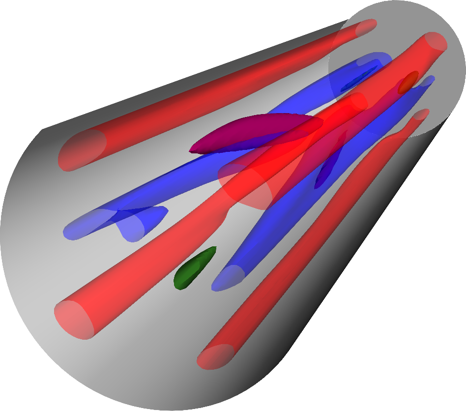 (b)
(b) 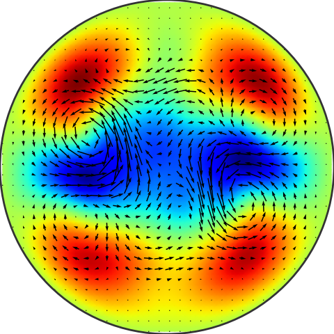 (c)
(c) 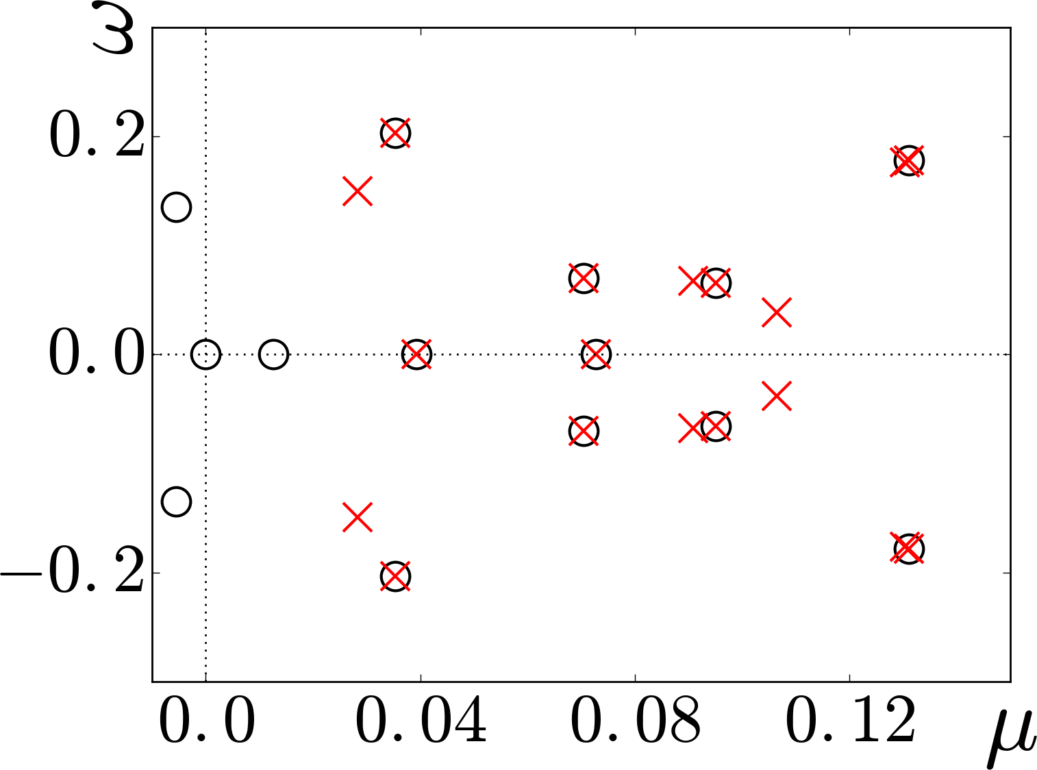
Figure 7(a,b) shows three- and two-dimensional visualizations of the new solution, which we hereafter refer to as S1N. While being on the laminar-turbulent boundary, S1N has a much more complicated structure compared to S1; its kinetic energy is roughly twice of it; and it has many more unstable directions. Solutions with similar properties were known (Faisst and Eckhardt, 2003; Wedin and Kerswell, 2004; Duguet et al., 2008; Pringle et al., 2009), mostly with higher azimuthal symmetries. However, none of the previously known solutions’ relevance to the full problem (without imposed symmetries) were established. Similarities between the initial condition’s figure 6 (c) and the converged state’s flow structures figure 7 (b) are apparent. Note particularly the locations of the vortical structures, which align very well. Since these structures do not extend along the pipe axis like streaks do, their one-to-one comparison is made possible by reduction to the translation-reduced state space (14).
As shown in figure 7 (c), S1N’s unstable manifold is 11-dimensional in the shift-and-reflect subspace and more unstable eigenvalues were found when the symmetry restriction was lifted. This renders a complete computational study of its unstable manifold impractical. Therefore on figure 8, we visualize two-dimensional surfaces associated with each of the leading three complex unstable eigenvalues in the full state space as the first application of symmetry reduction in both and .
(a) 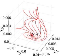 (b)
(b) 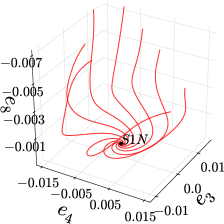 (c)
(c) 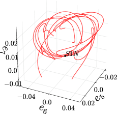
Let and respectively be complex eigenvalues and eigenvectors of S1N. Set of trajectories that approximately covers the linearized dynamics in the local two-dimensional plane spanned by are given by
| (32) |
In (32), is a small number and implies that state space points and eigenvectors are transformed into the first Fourier mode slice via (17) and (22) respectively. Under the linearized dynamics, a small perturbation to in direction expands by at one return of the spiral. Thus, the trajectories starting from the initial conditions (32) approximately satisfy , covering the associated two-dimensional surface. Using this approximation, we visualized time-forward dynamics of -surfaces associated with , , and on figure 8 (a, b, c) respectively. We assume that the eigenvalues are ordered from most unstable to the least i.e. Note that complex eigenvalues and eigenvectors satisfy , , , , , , where stands for complex conjugation. Projection bases , , are generated from , , and as follows: By definition, is a stability eigenvector with eigenvalue . If we choose
| (33) |
and become orthogonal i.e. . Projection bases are formed from these vectors as for . These bases fully capture local two-dimensional dynamics. We chose the third projection direction by trial and error to capture as much as possible as the trajectories develop into turbulence: and . is the real unstable eigenvector of S1N with largest real eigenvalue and is the leading eigenvector of S1. We have already illustrated in section III.2 that the direction corresponds to the trajectories in the vicinity of S1, which either laminarize or become turbulent and we are going to demonstrate that takes the same role for S1N.
Openpipeflow normalizes stability eigenvectors such that their norms are equal to that of the associated solution, i.e. . For computations of figure 8, we set (a, b) and (c); and picked equidistant point in for . While the spiral-out dynamics is clearly visible on figure 8 (a) and (b), trajectories look less organized on panel (c). This is because the imaginary part of the fifth eigenvalue is rather small, rendering the time for the trajectories to complete a full spiral long. This is not the case for and . While we might have obtained a better representation of the manifold in figure 8(c) if we had used more trajectories to represent it, we chose to leave it as it is in order to illustrate the possible shortcomings of the method. All trajectories in figure 8 eventually become turbulent, illustrating the rich dynamics that the laminar-turbulent boundary can exhibit.
In the full state space, the leading stability eigenvalues of S1N are complex conjugate (figure 7 (c)) and is purely real. In Figure 9 (a), we show the time-evolution of the kinetic energy when S1N is perturbed in the direction. As one would expect from a solution on the laminar-turbulent boundary, the flow relaminarizes in one direction while becoming turbulent in the opposite. While this observation clearly shows that S1N also belongs to the laminar-turbulent boundary, whether or not if its presence influences generic edge trajectories is not known. In the next section, we investigate this through a numerical experiment.
(a) 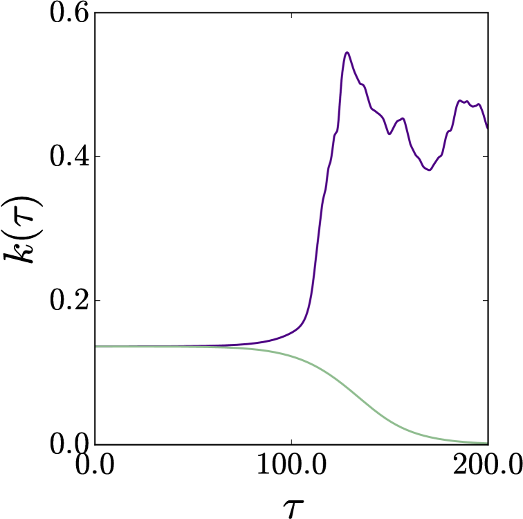
(b) 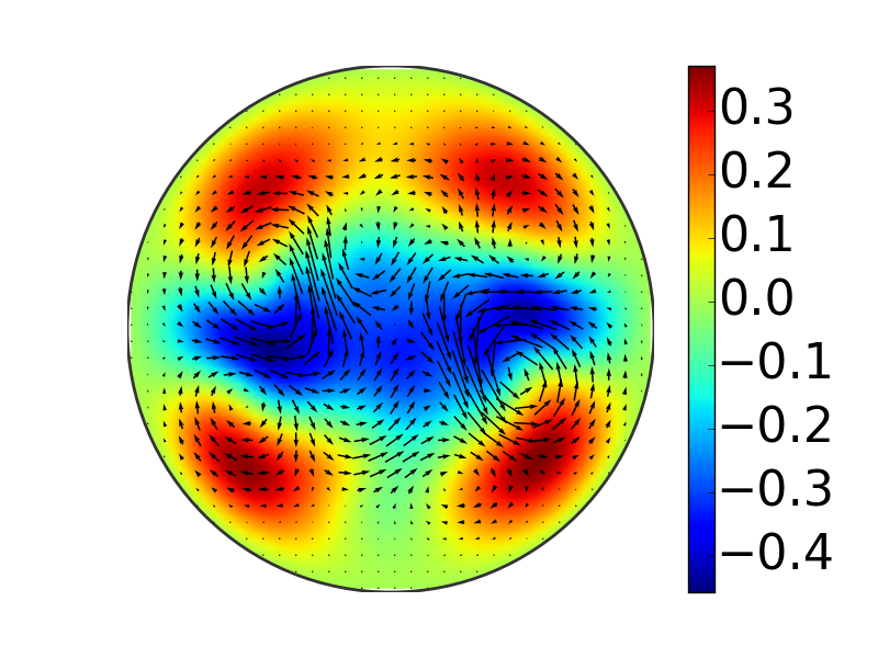 (c)
(c) 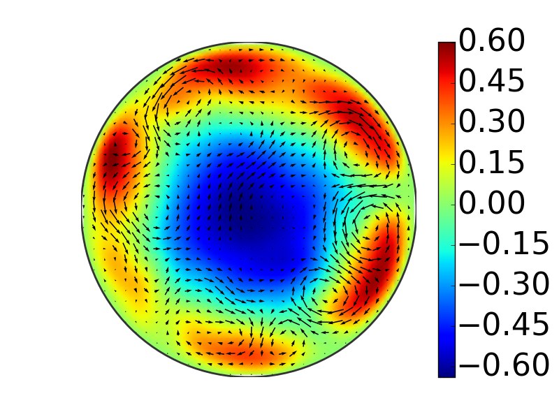
(d) 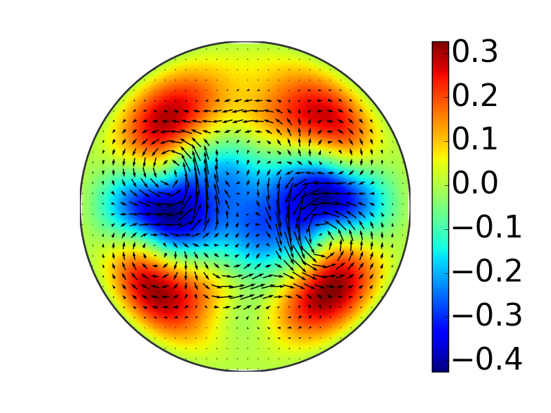 (e)
(e) 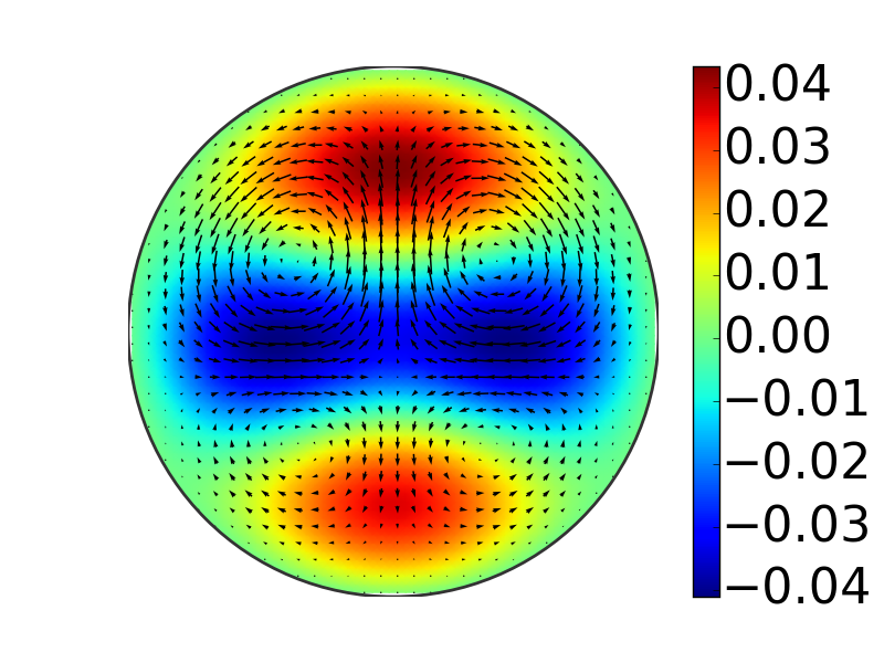
III.3 Approaches to the traveling waves
In order to illustrate how a generic trajectory on the laminar-turbulent is influenced by the traveling wave solutions present in the edge state, we carried out an edge tracking Itano and Toh (2001); Skufca et al. (2006) experiment where we bisected between initial conditions that become turbulent and those that laminarize. For this purpose, we randomly took a typical turbulent state at , scaled this field down by constants and and used these states as initial conditions at . After observing that the former uneventfully proceeds towards the laminar solution while the latter triggers turbulence, we began generating new initial conditions by bisecting in until we reached the limit of our numerical precision, such that the resulting trajectories stay in the laminar-turbulent boundary for longer and longer times. Kinetic energy time-series of these trajectories are shown in figure 10 (a). Such initial conditions are expected to approach to the invariant edge state Schneider et al. (2007) irrespective of how the very first state is generated. Therefore our choice of initial state from is arbitrary and many other initial states would approach to the edge state following the same algorithm.
(a) 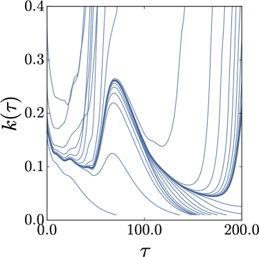 (b)
(b) 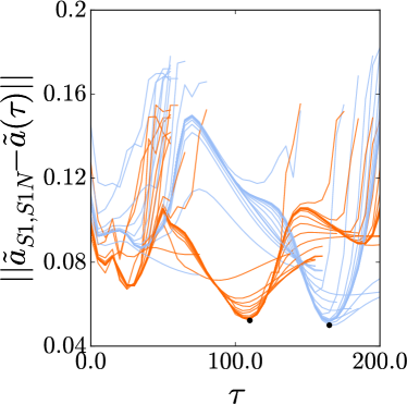
For every trajectory we generated through edge-tracking we the sampled flow states at intervals of and brought these states to the first Fourier mode slice through (17). We then measured distances of these states from S1 and S1N within the first Fourier mode slice. -distances of edge tracking trajectories from S1 and S1N are shown blue and orange respectively in figure 10(b), where each set of curves have a clear minimum marked with a black dot. We visualized these closest approaches next to the traveling waves they approach to in figure 11. Similarities between the flow structures of the traveling waves and the edge trajectories near them are clear, although the correspondence is not one-to-one.
(a) 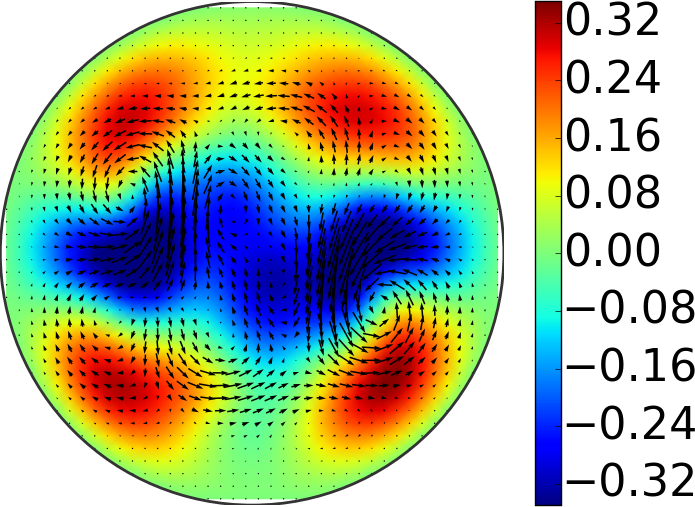 (b)
(b) 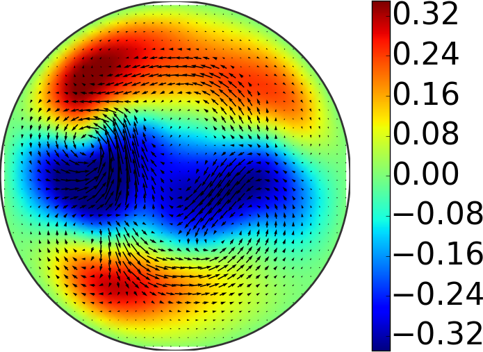 (c)
(c) 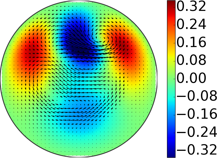 (d)
(d) 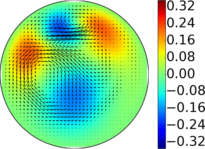
Notice that without the symmetry-reduction, such an analysis would have required an optimization over axial translations and azimuthal rotations for each step in order to minimize the distance between two states. Symmetry-reduction eliminates this step, decreasing the computational cost of the analysis tremendously.
IV Conclusion and outlook
In this paper, we introduced a representation of the pipe flow, where the continuous symmetries in axial and azimuthal directions are simultaneously reduced. This technical step was a straightforward extension of the first Fourier mode slice implementation of ref. Budanur and Hof (2017). Nevertheless, it was not implemented before and it successfully closes the continuous symmetry reduction problem for pipe flow. Adapting this method to other canonical shear flows is straightforward. For instance, in a channel geometry, the role of axial and azimuthal coordinates are taken over by streamwise and spanwise coordinates; and one should only make a choice for the wall-normal dependence of the template functions. Since this choice is somewhat arbitrary, a convenient option could be the first Chebyshev polynomial that is often used for numerical discretization in this direction.
For the application, we decided to revisit the laminar-turbulent boundary in a short () periodic computational cell of the pipe flow. Our first calculation that approximated the unstable manifold of S1 was very similar to that of Duguet et al. Duguet et al. (2008), who conjectured that the unstable manifold of S1 reached the neighborhoods of its own azimuthally rotated copies when it is followed along the laminar-turbulent boundary. Differently from ref. Duguet et al. (2008), we restricted our computation of the unstable manifold into the shift-and-reflect invariant subspace, to which the unstable manifold belongs. In addition, we visualized the unstable manifold as low-dimensional projections from the first Fourier mode slice (14). We found numerical evidence that the portion of this unstable manifold that is confined in the laminar-turbulent boundary visits the neighborhood of a new traveling wave, which we named S1N. Linear stability spectrum figure 7(c) showed that S1N has a very high dimensional unstable manifold, albeit being on the laminar-turbulent boundary. By visualizing two-dimensional surfaces associated with leading three complex conjugate unstable eigenvectors on figure 7, we illustrated variety of paths from the edge state leading to the turbulence. Besides demonstrating the utility of the symmetry reduction in both and , this computation also shows how rich the dynamics on the laminar-turbulent boundary can be. One main message we would like to deliver with the aid of these illustrations is that the asymptotic dynamics on the laminar-turbulent boundary in pipe flow should not be treated as a single state; but the edge state contains different regions with qualitatively different dynamics dictated by the nearby invariant solutions.
Both traveling waves we studied in this paper belonged to the shift-and-reflect invariant subspace of the pipe flow. One might argue against their relevance for the dynamics in the laminar-turbulent boundary since generic trajectories live in the full state space. Cvitanović et al. Cvitanović et al. (2009) nicely illustrates for one-dimensional Kuramoto-Sivashinsky system that the unstable manifolds of equilibrium solutions, all of which belong to the reflection invariant subspace, successfully captures the qualitative dynamics in the full state space of the -equivariant system. Our case here is similar to theirs since the symmetry in the azimuthal direction is also . Therefore, it is quite reasonable to expect for S1’s unstable manifold to form the backbone of the asymptotic dynamics on the laminar-turbulent boundary, given all the evidence that the edge state is located in its vicinity. Indeed, visualizations of figure 11 clearly show the similarities between the full state space trajectories and the traveling waves nearby.
Recently, Suri et al. Suri et al. (2017) studied the weakly turbulent quasi-two-dimensional flow experimentally and numerically. They demonstrated that when a turbulent trajectory comes close to an equilibrium, it leaves this neighborhood by following the unstable manifold of the solution. The tools we presented here, in particular, the methods for approximating and visualizing the unstable manifolds after symmetry-reduction, pave the way for a similar analysis in three-dimensional pressure-driven flows, which have traveling wave solutions rather than equilibria.
As we have shown in section III.3, symmetry-reduction frees us from reduced metrics, such as energy input or dissipation, that do not carry all information of the state space, and allows for measuring distances in the full state space. However, one should always keep in mind that two points that are at a short distance in the state space of a nonlinear system might evolve towards completely different regions. In order to conclusively answer whether or not a state space trajectory is “guided” by a particular unstable manifold, we should measure distances between curves in the state space, rather than points. While the finite-dimensional projections such as figures 4, 5, and 8 serve this purpose, they do not provide a complete picture of the infinite-dimensional state space. We believe developing computationally feasible methods for comparing shapes in high-dimensional state spaces is an important future problem for turbulence studies.
Acknowledgements.
We would like to acknowledge stimulating discussions with Yohann Duguet and Predrag Cvitanović. This research was supported in part by the National Science Foundation under Grant No. NSF PHY11-25915.References
- Meseguer and Trefethen (2003) A Meseguer and L. N Trefethen, “Linearized pipe flow to Reynolds number ,” J. Comput. Phys. 186, 178–197 (2003).
- Faisst and Eckhardt (2003) H. Faisst and B. Eckhardt, “Traveling waves in pipe flow,” Phys. Rev. Lett. 91, 224502 (2003).
- Pringle and Kerswell (2007) C. C. T. Pringle and R. R. Kerswell, “Asymmetric, helical, and mirror-symmetric traveling waves in pipe flow,” Phys. Rev. Lett. 99, 074502 (2007).
- Pringle et al. (2009) C. C. T. Pringle, Y. Duguet, and R. R. Kerswell, “Highly symmetric travelling waves in pipe flow,” Phil. Trans. Royal Soc. A 367, 457–472 (2009), arXiv:0804.4854.
- Schneider et al. (2007) T. M. Schneider, B. Eckhardt, and J. Yorke, “Turbulence, transition, and the edge of chaos in pipe flow,” Phys. Rev. Lett. 99, 034502 (2007).
- Duguet et al. (2008) Y. Duguet, A. P. Willis, and R. R. Kerswell, “Transition in pipe flow: the saddle structure on the boundary of turbulence,” J. Fluid Mech. 613, 255–274 (2008), arXiv:0711.2175.
- Mellibovsky et al. (2009) F. Mellibovsky, A. Meseguer, T. M. Schneider, and B. Eckhardt, “Transition in localized pipe flow turbulence,” Phys. Rev. Lett. 103, 054502 (2009).
- Hopf (1948) E. Hopf, “A mathematical example displaying features of turbulence,” Commun. Pure Appl. Math. 1, 303–322 (1948).
- Itano and Toh (2001) T. Itano and S. Toh, “The dynamics of bursting process in wall turbulence,” J. Phys. Soc. Japan 70, 701–714 (2001).
- Toh and Itano (2003) S. Toh and T. Itano, “A periodic-like solution in channel flow,” J. Fluid Mech. 481, 67–76 (2003).
- Schneider et al. (2008) T. M. Schneider, J. F. Gibson, M. Lagha, F. De Lillo, and B. Eckhardt, “Laminar-turbulent boundary in plane Couette flow,” Phys. Rev. E. 78, 037301 (2008), arXiv:0805.1015.
- Schneider et al. (2010) T. M. Schneider, D. Marinc, and B. Eckhardt, “Localized edge states nucleate turbulence in extended plane Couette cells,” J. Fluid Mech. 646, 441–451 (2010).
- Zammert and Eckhardt (2014) S. Zammert and B. Eckhardt, “A spotlike edge state in plane Poiseuille flow,” PAMM 14, 591–592 (2014).
- Khapko et al. (2016) T. Khapko, T. Kreilos, P. Schlatter, Y. Duguet, B. Eckhardt, and D. S. Henningson, “Edge states as mediators of bypass transition in boundary-layer flows,” J. Fluid Mech. 801 (2016), 10.1017/jfm.2016.434.
- Cvitanović et al. (2015) P. Cvitanović, R. Artuso, R. Mainieri, G. Tanner, and G. Vattay, Chaos: Classical and Quantum (Niels Bohr Inst., Copenhagen, 2015) ChaosBook.org.
- Kawahara and Kida (2001) G. Kawahara and S. Kida, “Periodic motion embedded in plane Couette turbulence: Regeneration cycle and burst,” J. Fluid Mech. 449, 291–300 (2001).
- Viswanath (2007) D. Viswanath, “Recurrent motions within plane Couette turbulence,” J. Fluid Mech. 580, 339–358 (2007), arXiv:physics/0604062.
- Ritter et al. (2016) P. Ritter, F. Mellibovsky, and M. Avila, “Emergence of spatio-temporal dynamics from exact coherent solutions in pipe flow,” New J. Phys. 18, 083031 (2016).
- Gibson et al. (2008) J. F. Gibson, J. Halcrow, and P. Cvitanović, “Visualizing the geometry of state space in plane Couette flow,” J. Fluid Mech. 611, 107–130 (2008), arXiv:0705.3957.
- Budanur and Hof (2017) N. B. Budanur and B. Hof, “Heteroclinic path to spatially localized chaos in pipe flow,” J. Fluid Mech 827, R1 (2017), 10.1017/jfm.2017.516.
- Willis (2017) A. P. Willis, “The Openpipeflow Navier-Stokes solver,” SoftwareX 6, 124 – 127 (2017).
- Wedin and Kerswell (2004) H. Wedin and R. R. Kerswell, “Exact coherent structures in pipe flow: Traveling wave solutions,” J. Fluid Mech. 508, 333–371 (2004).
- Budanur et al. (2017) N. B. Budanur, K. Y. Short, M. Farazmand, A. P. Willis, and P. Cvitanović, “Relative periodic orbits form the backbone of turbulent pipe flow,” J. Fluid Mech 833 (2017), 10.1017/jfm.2017.699.
- Willis et al. (2013) A. P. Willis, P. Cvitanović, and M. Avila, “Revealing the state space of turbulent pipe flow by symmetry reduction,” J. Fluid Mech. 721, 514–540 (2013), arXiv:1203.3701.
- Budanur et al. (2015a) N. B. Budanur, P. Cvitanović, R. L. Davidchack, and E. Siminos, “Reduction of the SO(2) symmetry for spatially extended dynamical systems,” Phys. Rev. Lett. 114, 084102 (2015a).
- Budanur et al. (2015b) N. B. Budanur, D. Borrero-Echeverry, and P. Cvitanović, “Periodic orbit analysis of a system with continuous symmetry - a tutorial,” Chaos 25, 073112 (2015b), arXiv:1411.3303.
- Froehlich and Cvitanović (2012) S. Froehlich and P. Cvitanović, “Reduction of continuous symmetries of chaotic flows by the method of slices,” Commun. Nonlinear Sci. Numer. Simul. 17, 2074–2084 (2012), arXiv:1101.3037.
- Cvitanović et al. (2012) P. Cvitanović, D. Borrero-Echeverry, K. Carroll, B. Robbins, and E. Siminos, “Cartography of high-dimensional flows: A visual guide to sections and slices,” Chaos 22, 047506 (2012).
- Rowley and Marsden (2000) C. W. Rowley and J. E. Marsden, “Reconstruction equations and the Karhunen-Loéve expansion for systems with symmetry,” Physica D 142, 1–19 (2000).
- Chossat and Lauterbach (2000) P. Chossat and R. Lauterbach, Methods in Equivariant Bifurcations and Dynamical Systems (World Scientific, Singapore, 2000).
- Armbruster et al. (1988) D. Armbruster, J. Guckenheimer, and P. Holmes, “Heteroclinic cycles and modulated travelling waves in systems with O(2) symmetry,” Physica D 29, 257–282 (1988).
- de Lozar et al. (2012) A. de Lozar, F. Mellibovsky, M. Avila, and B. Hof, “Edge state in pipe flow experiments,” Phys. Rev. Lett. 108, 214502 (2012).
- Krauskopf et al. (2005) B. Krauskopf, H. M. Osinga, E. J. Doedel, M. E. Henderson, J. Guckenheimer, A. Vladimirsky, M. Dellnitz, and O. Junge, “A survey of methods for computing (un)stable manifolds of vector fields,” Int. J. Bifurc. Chaos 15, 763–791 (2005).
- Skufca et al. (2006) J. D. Skufca, J. A. Yorke, and B. Eckhardt, “Edge of Chaos in a parallel shear flow,” Phys. Rev. Lett. 96, 174101 (2006).
- Cvitanović et al. (2009) P. Cvitanović, R. L. Davidchack, and E. Siminos, “On the state space geometry of the Kuramoto-Sivashinsky flow in a periodic domain,” SIAM J. Appl. Dyn. Syst. 9, 1–33 (2009), arXiv:0709.2944.
- Suri et al. (2017) B. Suri, J. Tithof, R. O. Grigoriev, and M. F. Schatz, “Forecasting fluid flows using the geometry of turbulence,” Phys. Rev. Lett. 118, 114501 (2017), arXiv:1611.02226.