Multiplex Influence Maximization in Online Social Networks with Heterogeneous Diffusion Models

Abstract

Motivated by online social networks that are linked together through overlapping users, we study the influence maximization problem on a multiplex, with each layer endowed with its own model of influence diffusion. This problem is a novel version of the influence maximization problem that necessitates new analysis incorporating the type of propagation on each layer of the multiplex. We identify a new property, generalized deterministic submodular, which when satisfied by the propagation in each layer, ensures that the propagation on the multiplex overall is submodular – for this case, we formulate ISF, the greedy algorithm with approximation ratio $(1-1/e)$. Since the size of a multiplex comprising multiple OSNs may encompass billions of users, we formulate an algorithm KSN that runs on each layer of the multiplex in parallel. KSN takes an $\alpha$-approximation algorithm $A$ for the influence maximization problem on a single network as input, and has approximation ratio $\frac{(1-\epsilon)\alpha}{(o+1)k}$ for arbitrary $\epsilon>0$, $o$ is the number of overlapping users, and $k$ is the number of layers in the multiplex. Experiments on real and synthesized multiplexes validate the efficacy of the proposed algorithms for the problem of influence maximization in the heterogeneous multiplex. Implementations of ISF and KSN are available at http://www.alankuhnle.com/papers/mim/mim.html.

I Introduction

The rapid growth of large Online Social Networks (OSN) such as Facebook, Google+, and Twitter has enabled them to become thriving places for viral marketing in recent years. People are increasingly engaged in OSNs: 62% of adults worldwide use social media and spend 22% of online time on social networks on average [1]. Much like real-world social networks, information spreading in OSNs has viral properties, creating an excellent medium for marketing. Due to the impact of this effect on the popularity of new products, OSNs have rapidly become an attractive channel for raising awareness of new products or brands. In this context, an important problem is how to find the best set of seed users who can influence the most other users.

Increasingly, users engage in more than one OSN; they connect their accounts across multiple networks, such that posts in one network are simultaneously posted in other networks. In Fig. 1, we show the process of connecting a Facebook and Twitter account, which allows automatically posting on Facebook when a new tweet is sent, and vice versa. As a consequence, the propagation of information can cross from one OSN to another through these overlapping users.

The influence propagation in each OSN will be particular to that network; for example, usage patterns for Twitter and Facebook are quite different. Moreover, even different cascades in the same social network may be better explained by different models of influence propagation [2]. Thus, overlapping users connect OSNs together into a multiplex structure of OSNs, comprising multiple OSNs linked together through overlapping users, where each OSN has different local propagation. In this work, we study the multiplex influence maximization (MIM) problem, to pick the most influential seed nodes, on a multiplex of OSNs as described above. Several natural questions arise: (1) what conditions on the propagation in each layer OSN are sufficient for the overall multiplex propagation to have the submodularity property, which is important for approximation algorithms? (2) Can existing methods for single OSNs be utilized within a solution to the MIM problem? (3) What role do overlapping users play in the influence propagation on a multiplex of OSNs? From a computational perspective, a multiplex consisting of multiple OSN layers may be very large, comprising billions of users in each layer.

(a) Auto-post from Twitter to Facebook

(b) Auto-post from Facebook to Twitter

Figure 1: The process of becoming an overlapping user of Twitter and Facebook.

Figure 2: A 2-layer multiplex exemplifying how propagation in a multiplex will deviate from the propagation in a single layer.

To demonstrate how propagation in a multiplex differs from propagation in a single layer, consider the toy multiplex shown in Fig. 2, where $a,b$ are overlapping users in both layers, and $c$ is only present in Layer 1. Let Layer 1 have a fixed threshold model, with the threshold $\theta_{c}$ of $c$ equal to 1. Thus, $c$ becomes activated iff $a,b$ are both activated. Let Layer 2 have the Independent Cascade (IC) model. Then seeding vertex $a$ will result in both $b,c$ having a chance of becoming activated, as $a$ may activate $b$ according to the IC model in Layer 2. If $b$ becomes activated, then $a,b$ will together activate $c$ in Layer 1. Finally, observe that the activation of the two layers cannot be incorporated into a single layer network following either the IC model or the fixed threshold model.

For influence maximization problem on a single layer network with propagation according to a single model, such as Independent Cascade (IC), approximation algorithms have been developed and optimized [3, 4, 5, 6, 7]. However, since these algorithms only consider a single model of influence propogation, they are not directly suitable for MIM, where each OSN has a different model of propagation. As shown in Fig. 3, the fraction of overlapping users is considerable.

-	LinkedIn	Facebook	Twitter	MySpace
LinkedIn	-	$12\%$	$21\%$	$6\%$
Facebook	$82\%$	-	$91\%$	$57\%$
Twitter	$31\%$	$20\%$	-	$17\%$
MySpace	$36\%$	$49\%$	$70\%$	-

Figure 3: The percentage of overlapping users between major OSNs in 2009 [8]. The table is read as follows: $(x,y)\%$ of users in OSN $y$ also use OSN $x$, where $x$ is the row, $y$ is the column

Our main contributions are summarized as follows.

• We define the generalized deterministic submodular (GDS) property, which if satisfied by each layer implies overall propagation on the multiplex is submodular. Submodularity allows the formulation of a greedy $(1-1/e)$-approximation algorithm (ISF) for MIM.

• We provide an approximation algorithm Knapsack Seeding of Networks (KSN) which is parallelizable by layer of the multiplex and utilizes an algorithm $\mathcal{A}$ for the single-layer influence maximization problem together with a knapsack-based approach to create a solution for MIM, thereby taking advantage of previous optimizations [4, 5, 6, 7] for the homogeneous, single layer case. If the utilized algorithm $\mathcal{A}$ has approximation factor $\alpha$, then KSN has approximation ratio

  $$\frac{(1-\epsilon)\alpha}{(o+1)k},$$

  where $o$ is the number of overlapping users in the multiplex, $k$ is the number of layers in the multiplex, and $\epsilon>0$ is arbitrary.

• Experimental evaluation of all algorithms on a variety of multiplexes, both synthesized and from traces of real multiplexes of OSNs, validates the effectiveness of the two approximation algorithms.

Overlapping users can be identified in real networks using, for example, methods in [9, 10]; methods of identification is not a focus of this paper.

The rest of the paper is organized as follows. In Section II, we provide technical definition for model of influence propagation. Also, we present the influence propagation model in multiplex networks in terms of its component layers and define the problem. We then outline our proposed algorithms for solving the MIM problem along with the inapproximability proof for a class of models in Section III. Section IV shows the experimental results on the performance of different algorithms. In Section V we discuss related work on influence propagation and finally, Section VI concludes the paper.

II Model Representation and Problem Formulation

II-A Influence Propagation Models

Intuitively, the idea of a model of influence propagation in a network is clear; it is a way by which nodes can be activated or influenced given a set of seed nodes. Kempe et al. studied a variety of models in their seminal work on influence progation on a graph, including the Independent Cascade (IC) and Linear Threshold (LT) models [11]. For completeness, we briefly describe these two models. An instance of influence propagation on a graph $G$ follows the IC model if a weight can be assigned to each edge such that the propagation probabilities can be computed as follows: once a node $u$ first becomes active, it is given a single chance to activate each currently inactive neighbor $v$ with probability proportional to the weight of the edge $(u,v)$. In the LT model each network user $u$ has an associated threshold $\theta(u)$ chosen uniformly from $[0,1]$ which determines how much influence (the sum of the weights of incoming edges) is required to activate $u$. $u$ becomes active if the total influence from its direct neighbors exceeds the threshold $\theta(u)$.

In this work, since we allow each layer of a multiplex to have a different model of influence propagation, we need a technical definition for this concept.

Definition 1 (Model of influence propagation).

A model of influence propagation $\sigma$ on a graph $G=(V,E)$ is a function $P$ that assigns, for each $A\subset V$, and for each $S\subset V$, a probability

$$P(S|A)=P(S\text{ is final activated set }|A\text{ is seed set })\in[0,1],$$

satisfying

$$(1)\text{ if }B\cap A\subsetneq A,P(B|A)=0,$$

$$(2)\sum_{S:S\subset V}P(S|A)=1.$$

(1) simply states that seed nodes may not become unactivated, and (2) ensures that we have a probability distribution.

The expected number of activated nodes given a seed set $A$ is denoted $\sigma(A)$, and

$$\sigma(A)=\sum_{S:S\subset V}P(S|A)\cdot|S|.$$

A model $\sigma$ is called deterministic iff for each $A\subset V$, there exists $F_{A}$ such that $P(F_{A}|A)=1$; intuitively, deterministic means that there is no probability in the model of diffusion, since the final set activated is uniquely determined by the seed set. If $\sigma$ is deterministic, $\sigma(A)=|F_{A}|$; we abuse notation and also use $\sigma(A)=F_{A}$, the final set itself. This allows convenient specification of the set $T=\sigma(\tau(A))$, for example, where both $\sigma,\tau$ are deterministic models, and $T$ is the final activated set generated by using the final set of $A$ under $\tau$ as the seed set for $\sigma$.

Many models of information propagation discussed in the literature satisfy the submodularity property, that $\sigma$ satisfies

$$\sigma(A)+\sigma(B)\geq\sigma(A\cup B)+\sigma(A\cap B),$$

for all $A,B\subset V$. Submodularity is important since it guarantees that a greedy approach to the influence maximization prolem will have an approximation ratio [12]. We now define a property that is stronger than submodularity.

Definition 2 (Generalized Deterministic Submodular).

Let $\sigma$ be a model of influence propagation. $\sigma$ satisfies the generalized deterministic submodular property (GDS) if the expected number of activations, given seed set $A$, can be written

$$\sigma(A)=\sum_{j=1}^{s}p_{j}\sigma_{j}(A),$$

where each $\sigma_{j}$, $j\in\{1,\ldots,s\}$ is a deterministic, submodular model of influence propagation, and $p_{j}\in[0,1]$, $\sum_{j=1}^{s}p_{j}=1$.

Lemma 1.

Let $\sigma$ be a model of influence propagation. If $\sigma$ satisfies GDS, then $\sigma$ is submodular.

Proof.

Let $A$ be an arbitrary seed set. Since $\sigma$ satisfies GDS, $\sigma(A)=\sum_{i=1}^{s}p_{j}\sigma_{j}(A)$, where $\sigma_{j}(A)$ is expected activation of deterministic and submodular model $\sigma_{j}$. Hence the expected activation function $\sigma$ is a nonnegative linear combination of submodular functions, thus $\sigma$ is submodular. ∎

Examples of models in the literature that satisfy submodularity include IC, LT, Asynchronous Independent Cascade, Asynchronous Linear Threshold [13], Independent Cascade Model for Endogenous Competition, Homogeneous Competitive Independent Cascade model, and K-LT competitive diffusion model, as well as others [11] [14]. In all cases, the submodularity of these models has been shown by considering instances where some edges are live and some are blocked – each such instance corresponds to a deterministic submodular model. Thus, all of these proofs show submodularity by showing the stronger property GDS and using Lemma 1. Another example of a model that satisfies GDS is the conformity and context-aware cascade model [15].

In section III, we show (Theorem 1) that influence propagation on a multiplex satisfies GDS if the propagation on each layer network satisfies GDS; hence if the propagation on each layer satisfies GDS, the propagation in the multiplex is submodular.

II-B Notations and Multiplex Model

A social network can be modeled as a directed graph $G=(V,E)$. The vertex set $V$ represents the participation of users in the social network, and the edge set represents the connections among network users. These connections model friendships or relationships.

Definition 3 (Heterogeneous multiplex).

A multiplex of OSNs is a list $\mathscr{G}=\{(G_{i},\sigma_{i}):i\in\{1,\ldots,k\}\}$ with $G_{i}=(V_{i},E_{i})$ a directed graph representing an OSN and influence model $\sigma_{i}$, representing the model of influence propagation in $G_{i}$. If a user belongs to more than one OSN, an interlayer edge is added between the pair of nodes, one in each OSN, representing this user. Such a user is termed overlapping user; we will denote the set of overlapping users by $O$. We will denote the set of all users in the multiplex by $V=\bigcup_{i=1}^{k}V_{i}$.

The influence propagation model $\sigma$ on the multiplex is defined in the following way. If an overlapping vertex $v$ is activated in one graph $G_{i}$, then, deterministically its adjacent interlayer copies become activated in all OSNs; propagation occurs in each graph $G_{i}$ according to its propagation model $\sigma_{i}$. Figure 4 shows an example of the definition of $\sigma$, in a multiplex $\mathscr{G}=\{(G_{1},\sigma_{1}),(G_{2},\sigma_{2})\}$ with two layers. Here $\sigma_{1}$ and $\sigma_{2}$ are simply deterministic models of activation following the directed edges in the layers. Initially, the activated set is $\{v_{1},v_{6}\}$ in Fig. 4(a), shown by red nodes. In 4(b), the activation has propagated according to $\sigma_{1},\sigma_{2}$ in $G_{1},G_{2}$, respectively, activating in addition set $\{v_{2},v_{3},v_{8}\}$. Next, in 4(c), the propagation proceeds between the two layers via overlapping nodes, whereupon it may continue in each layer $G_{i}$ according to $\sigma_{i}$. Propagation ceases when no new nodes are activated in any layer. In addition, Fig. 4 demonstrates how without loss of generality, we may consider all nodes to be overlapping by adding absent nodes as isolated nodes (the white nodes). In section III-A1, we make use of this fact by considering all layers to have the same nodes – in the rest of the paper, we consider overlapping users to be non-trivial; i.e. there are no isolated nodes in any layer. We refer to the users that actively participate in multiple networks (i.e. are non-isolated) as overlapping users, which may be identified in real networks using, for example, methods in [9, 10].

The expected number of activations in the multiplex given seed set $A\subset V$ is denoted $\sigma(A)$, in addition to denoting the model defined above as $\sigma$; we do not count more than one copy of overlapping nodes towards $\sigma(A)$. Each graph $G_{i}$ is referred to as a layer network of the multiplex $G$. We refer to a graph $G=(V,E)$ that is not part of a multiplex as a single network, to contrast with multiplex network, and we refer to propagation occuring in a single network according to a single influence propagation model as homogeneous propagation, to contrast with the heterogeneous propagation in a multiplex with more than one layer and propagation model in each layer.

II-C Problem Definition

We now consider the problem of maximizing the influence of a seed set of given size in a multiplex network. Formally,

Definition 4 (Heterogeneous Multiplex Influence Maximization (MIM)).

Given a multiplex network $\mathscr{G}=(G_{1},\sigma_{1}),\ldots,(G_{k},\sigma_{k})$ with $k$ layer networks, influence propagation model $\sigma$ on $\mathscr{G}$, as defined above in terms of $\sigma_{i}$, and positive integer $l$, find a set $S\subset V$ of size at most $l$ so as to maximize the expected number of active users $\sigma(S)$. An instance of this problem will be denoted $(\mathscr{G},k,l,\sigma)$.

III Approximations of MIM

Since influence maximization on a single network is a special case of influence maximization on a multiplex, MIM is $NP$-complete. In this section, we first prove that the propagation $\sigma$ on a multiplex is submodular if the propagation on each layer satisfies GDS and formulate a greedy algorithm to maximize expected influence. If each layer satisfies GDS, $\sigma$ is submodular and thus our greedy algorithm has approximation ratio $1-1/e$. Finally, we consider approaches to approximate MIM by approximating influence maximization on each layer separately and effectively combining the result into a feasible solution for MIM, which leads to a scalable approximation algorithm KSN with ratio depending on number of overlapping users $o$, number of layers $k$ in the multiplex, the ratio $\alpha$ for the approximation used on the homogeneous layers, and an arbitrary $\epsilon>0$; the ratio of KSN is $\frac{(1-\epsilon)\alpha}{(o+1)k}$.

III-A Greedy approach

Let $\mathscr{G}=(G_{i},\sigma_{i})_{i=1}^{k}$ be a multiplex with propagation model $\sigma$. We prove that $\sigma$ is submodular for the case that each $\sigma_{i}$ satisfies generalized deterministic submodularity (GDS). Thus, the greedy algorithm, which we detail in this section, achieves a $(1-1/e)$ ratio when propagation in each layer $\sigma_{i}$ satisfies GDS.

III-A1 Submodularity

Without loss of generality, we may consider that the sets $V_{i}$ are the same; that is, $V_{i}=V$ for all $i$ and some set $V$: if a vertex $v\in G_{i}$ does not exist in some $G_{j}$, simply add it to $G_{j}$ as an isolated vertex. Thus, in this section only, we consider $V_{i}=V$ for all $i$. Recall that instead of counting the activation of all $k$ copies of node $u\in V$, we count only a single copy as activated. The expected number of activations in the multiplex given seed set $A\subset V$ is denoted $\sigma(A)$; again, we do not count more than one copy of $u\in V$ towards $\sigma(A)$.

We will first consider a simpler case: when the propagation of each $G_{i}$ is deterministic and submodular.

Deterministic case

In this section, let the propagation $\sigma_{i}$ of each $G_{i}$ be deterministic and submodular. Recall the definition of the multiplex influence propagation $\sigma$. Given a seed set $S\subset V$, the set of nodes in the multiplex that are activated after the propagation finishes will be denoted by $\tau(S)$; the nodes activated if propagation is restricted to only $G_{i}$ will be denoted $\tau_{i}(S)$. Notice that $|\tau(S)|=\sigma(S)$ and $|\tau_{i}(S)|=\sigma_{i}(S)$.

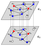
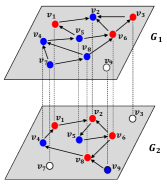
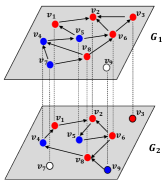
Figure 4: (a)–(c) An example of influence propagation $\sigma$ in the multiplex structure. Red nodes are activated, blue and white are unactivated nodes. The white color indicates a node added to the layer in order that each network has the same vertex set $V$. In (a), we have seed set conserting of $v_{1}$ and $v_{6}$. In (b), propagation occurs in each layer according to that layers model, and in (c), nodes activated in one layer are activated in all, whence the propagation may continue.

Lemma 2.

Let $S\subset V$. Then $\tau_{i}(\tau(S))=\tau(S)$ for all $i$.

Proof.

This follows from definition of propagation in multiplex. If propagation has resulted in set $\tau(S)$, then propagation cannot proceed further in any layer network, for otherwise propagation in $\mathscr{G}$ would not have terminated with $\tau(S)$. A visualization of an example of multiplex propagation is shown in Figure 4 (a)–(c). ∎

Lemma 3.

Let $S,T\subset V$.

$$\tau(S)\cup\tau(T)=\tau_{i}(\tau(S)\cup\tau(T))$$

for all $i$.

Proof.

We have

$$\sigma_{i}(\tau(S)\cup\tau(T))+\sigma_{i}(\tau(S)\cap\tau(T))\leq\sigma_{i}(\tau(S))+\sigma_{i}(\tau(T))$$

by submodularity of $\sigma_{i}$, so

$$\sigma_{i}(\tau(S)\cup\tau(T)) \leq|\tau(S)|+|\tau(T)|-|\tau(S)\cap\tau(T)|$$

$$=|\tau(S)\cup\tau(T)|,$$

by Lemma 2 and since $\sigma_{i}(\tau(S)\cap\tau(T))\geq|\tau(S)\cap\tau(T)|$. Hence,

$$\tau_{i}(\tau(S)\cup\tau(T))=\tau(S)\cup\tau(T).$$

∎

Lemma 4.

Let $S,T\subset V$.

• $$\tau(S\cup T)=\tau(S)\cup\tau(T)$$

• $$\tau(S\cap T)\subset\tau_{i}(\tau(S)\cap\tau(T)).$$

Proof.

• Since $S\cup T\subset\tau(S)\cup\tau(T)$, $\tau(S)\cup\tau(T)\subset\tau(S\cup T)$ and propagation in any layer network $G_{i}$ cannot procede beyond $\tau(S)\cup\tau(T)$ by Lemma 3, we have $\tau(S\cup T)=\tau(S)\cup\tau(T)$.

• Clearly $\tau(S\cap T)\subset\tau(S)$ and similarly $\tau(S\cap T)\subset\tau(T)$, hence

  $$\tau(S\cap T)\subset\tau(S)\cap\tau(T)\subset\tau_{i}(\tau(S)\cap\tau(T)),$$

  for any $i$.

∎

Lemma 5.

If the propagation model $\sigma_{i}$ on each component of $\mathscr{G}$ is deterministic and submodular, the (deterministic) propagation $\sigma$ in multiplex $\mathscr{G}$ will be submodular.

Proof.

Let $i\in\{1,\ldots,n\}$. Then by Lemmas 2, 3 and 4 and submodularity of $\sigma_{i}$,

$$\sigma(S\cap T)+\sigma(S\cup T) =|\tau(S\cap T)|+|\tau(S\cup T)|$$

$$\leq|\tau_{i}(\tau(S)\cap\tau(T))|+|\tau_{i}(\tau(S)\cup\tau(T))|$$

$$=\sigma_{i}(\tau(S)\cap\tau(T))+\sigma_{i}(\tau(S)\cup\tau(T))$$

$$\leq\sigma_{i}(\tau(S))+\sigma_{i}(\tau(T))$$

$$=\sigma(S)+\sigma(T).$$

Thus, $\sigma$ is submodular. ∎

Probabilistic case

Now the result for the deterministic case is generalized to the case when all networks satisfy GDS.

Theorem 1.

Given multiplex network $\mathscr{G}$ with $k$ layer networks $G_{i}$, if the model $\sigma_{i}$ on each layer network $G_{i}$ satisfies GDS then $\sigma$ satisfies GDS.

Proof.

Since $\sigma_{i}$ satisfies GDS, with probability $p_{ij}$, $G_{i}$ has deterministic, submodular propagation $\sigma_{ij}$, such that $\sigma_{i}=\sum p_{ij}\sigma_{ij}$. The probability that $\sigma$ will comprise $\sigma_{1j_{1}},\sigma_{2j_{2}},\ldots,\sigma_{kj_{k}}$ is $\prod_{i=1}^{k}p_{ij_{i}}$, since propagation in each graph is independent. Let this propagation in $\mathscr{G}$ be labeled $\sigma_{j_{1},\ldots,j_{k}}$. By Lemma 5, $\sigma_{j_{1},\ldots,j_{k}}$ is submodular and deterministic. ∎

III-A2 $(1-1/e)$-Approximation Algorithm

In this section we detail the greedy algorithm Influential Seed Finder (ISF) for solving the MIM problem. As shown in Alg. 1, ISF is a greedy algorithm (with CELF++ optimization [16]), which chooses a node that maximizes the marginal gain of $\sigma$ at each iteration. Recall that $\sigma$ is the expected activation of the influence model $\sigma$ defined on the multiplex in Section II, which incorporates the models $\sigma_{i}$ on each layer utilizing the overlapping users. To compute $\sigma$, it is necessary to compute expected activation $\sigma_{i}$ on each layer. To perform this computation, we use independent Monte Carlo simulations – in general, $\sigma_{i}$ could be any model of influence propagation, and thus may not be amenable to specialized techniques for triggering model [7].

As shown earlier, $\sigma$ is submodular and monotone increasing when each individual network satisfies GDS; therefore, in this case ISF has an approximation ratio of $(1-1/e)$ [12]. The time complexity of ISF is $O(nl(m+n)\log n)$ where $n,m$ are number of users, friendships in the multiplex of OSNs, respectively. Each Monte Carlo simulation takes time $\Omega(n+m)$, and the $\log n$ factor accounts for the time to adjust the priority queue, $l$ is the size of the seed set chosen.

Algorithm 1 ISF: An algorithm for finding the best seed users. Approximation ratio: $1-1/e$ when each layer satisfies GDS property

Input: A multiplex $\mathscr{G}=(G^{1},G^{2},\ldots,G^{k})$, $l$
Output: Seed set $S$ of size $l$

1:Renumber all the nodes across all networks so that each node gets a unique id

2:$S\leftarrow\emptyset$

3:$V\leftarrow\cup_{i=1}^{k}V_{i}$

4:for each $v\in V$ do

5:     $v.marginal\_gain=\sigma(v)$

6:     $v.round=0$

7:end for

8:Initialize max priority queue $Q$ with (key,value) pair $(v,v.marginal\_gain)$, $\forall v\in V$

9:Initialize previous marginal gain, $prev\_mg=0$

10:while $|S|\leq l$ do

11:     $v\leftarrow Q.pop().key$

12:     if $v.round==S.size$ then

13:         $S\leftarrow S\cup\{v\}$

14:         $prev\_mg\leftarrow prev\_mg+v.marginal\_gain$

15:     else

16:         $v.marginal\_gain\leftarrow\sigma(S\cup\{v\})-prev\_mg$

17:         $v.round=S.size$

18:         $Q.add(v,v.marginal\_gain)$

19:     end if

20:end while

21:Return $S$

III-B Parallelizable multiplex algorithm

Although in the case that the model of propagation on each layer satisfies GDS, we have the $(1-1/e)$ performance guarantee of the greedy ISF, the running time of ISF may be impractical for large network sizes; hence we propose Alg. 2 (KSN), another approximation algorithm which parallelizes the problem in terms of the component layers – the difficulty lies in combining the solutions to the influence maximization problem on the separate layers to obtain a solution for MIM. KSN achieves this by approximating the solution to multiple-choice knapsack problem. The approximation ratio of KSN depends on the number of overlapping users $o$, the number of layers $k$, an arbitrary $\epsilon>0$, and the ratio $\alpha$ of its input homogeneous layer algorithm $A$.

III-B1 Description of KSN

-	0	1	2	3	4
$G_{1}$	0	200	350	400	425
$G_{2}$	0	600	601	602	603
$G_{3}$	0	200	210	214	214

Figure 5: An example of how KSN works, as described in the text.

The KSN algorithm takes as input an algorithm $A$ (with ratio $\alpha$) to solve the influence maximization problem on a single layer network, a multiplex network $\mathscr{G}$ with $k$ layers, and number of seeds to pick $l$. For each $j\in\{1,\ldots,l\}$, $i\in\{1,\ldots,k\}$, algorithm $A$ is run in parallel on each $G_{i}$ to get seed sets $T_{ij}$ with $j$ seed nodes. It then uses an approximation to the multiple-choice knapsack problem (defined below) to decide how many nodes should be seeded in each layer, i.e. for each $i$, which $T_{ij}$ to pick.

For example, suppose we have a multiplex with three layers: $G_{1},G_{2},G_{3}$. Using algorithm $A$, we generate the table in Fig. 5, where the $(i,j)$th entry gives the activation of seeding $j$ nodes in layer $G_{i}$. We then use an algorithm for multiple-choice knapsack to choose for each layer $G_{i}$, the number $j_{i}$ of nodes to seed in that layer.

Algorithm 2 Knapsack Seeding of Networks (KSN): A knapsack approach to finding the best seed users. Approximation ratio: $\frac{(1-\epsilon)\alpha}{(o+1)k}$, where $\epsilon>0$, $o$ is the number of overlapping users, $k$ is the number of layers, and $\alpha$ is the ratio of algorithm $A$ on homogeneous networks

Input: Algorithm $A$, a multiplex network $\mathscr{G}=(G^{1},G^{2},\ldots,G^{k})$, $l$
Output: Seed set $T$ of size $l$

1:for $i\in\{1,\ldots k\}$ do

2:     Run algorithm $A$ on $G_{i}$ with input $j$ to get seed sets $T_{i1},T_{i2},\ldots,T_{il}\subset G_{i}$, with $|T_{ij}|=j$.

3:end for

4:For each $T_{ij}$, let cost $c(T_{ij})=|T_{ij}|$, and profit $p(T_{ij})=\sigma(T_{ij})$.

5:Use $(1-\epsilon)$-approximation to MCKP to choose for all $i$, $T^{\prime}_{i}\in\{T_{i1},\ldots,T_{il}\}$, which choice satisfies $\sum_{i=1}^{k}|T^{\prime}_{i}|=l$.

6:Return $T=\bigcup_{i}T^{\prime}_{i}$.

Worst-case bound on performance of KSN

First, we need the definition of the multiple-choice knapsack problem.

Definition 5 (Multiple-choice knapsack problem (MCKP)).

Let $(\mathscr{C},k,l,c,p,B)$ be given, where $\mathscr{C}=\{C_{1},\ldots C_{k}\}$ comprises $k$ classes of $l$ objects, $C_{i}=\{x_{ij}:1\leq j\leq l\}$, $c$ and $p$ are cost and profit functions on objects $x_{ij}$, and budget $B\geq 0$. The multiple-choice knapsack problem (MCKP) is to pick one item from each class, $x_{i}^{\prime}$ such that profit $\sum_{i=1}^{k}p(x_{i}^{\prime})$ is maximized under the constraint $\sum_{i=1}^{k}c(x_{i}^{\prime})<B$.

For $\epsilon>0$, MCKP has a $(1-\epsilon)$-approximation as shown in [17]. We will use this algorithm to obtain an approximation for MIM as follows. Let an instance $(\mathscr{G},k,l)$ of MIM be given. For each pair $(i,j)$, $1\leq i\leq k,1\leq j\leq l$, let $T^{opt}_{ij}$ be an optimal seed set for $G_{i}$ satisfying the two conditions $T^{opt}_{ij}\subset G_{i}$ and $|T^{opt}_{ij}|=j$. In addition, let $T_{ij}$ be the approximation from algorithm $A$ to $T^{opt}_{ij}$. That is, $T_{ij}\subset G_{i}$, $|T_{ij}|=j$, and

$$\sigma(T_{ij}^{opt})\leq\alpha^{-1}\sigma(T_{ij}).$$

Then let $C_{i}=\{T_{i0},\ldots,T_{il}\}$, $C^{opt}_{i}=\{T^{opt}_{i0},\ldots,T^{opt}_{il}\}$. Finally, let $\mathscr{C}=\{C_{i}:1\leq i\leq k\}$, $\mathscr{C}^{opt}=\{C_{i}^{opt}:1\leq i\leq k\}$, and for each $i,j$, define $c(T_{ij})=j$, $p(T_{ij})=\sigma(T_{ij})$, and likewise define $c,p^{opt}$ for each $T_{ij}^{opt}$. Thus, we have two instances of the knapsack problem, namely $I_{1}=(\mathscr{C},k,l,c,p,l)$ and $I_{2}=(\mathscr{C}^{opt},k,l,c,p^{opt},l)$.

Lemma 6.

Let $Opt_{I_{i}}$ be the value of the optimal solution to MCKP instance $I_{i}$, $i\in\{1,2\}$. Then

$$\alpha Opt_{I_{2}}\leq Opt_{I_{1}}.$$

Proof.

Suppose $\{T_{ib_{i}}:1\leq i\leq k\}$, $\{T^{opt}_{ia_{i}}:1\leq i\leq k\}$ are the optimal solutions for $I_{1},I_{2}$, respectively. Then

$$\alpha Opt_{I_{2}} =\alpha\sum_{i}\sigma(T^{opt}_{ia_{i}})$$

$$\leq\sum_{i}\sigma(T_{ia_{i}})$$

$$\leq\sum_{i}\sigma(T_{ib_{i}})$$

$$=Opt_{I_{1}},$$

since algorithm $A$’s selection of $T_{ia_{i}}$ ensures $\sigma(T_{ia_{i}})\geq\alpha\sigma(T^{opt}_{ia_{i}})$. The last inequality follows from the fact that $\{T_{ia_{i}}\}$ is a feasible solution to instance $I_{1}$, and $\{T_{ib_{i}}\}$ is the optimal solution to $I_{1}$. ∎

Theorem 2.

Let $A$ be an $\alpha$-approximation to the problem of influence maximization on a homogeneous single layer, and let $o,k$ be the number of overlapping users and layers, respectively in the multiplex. Furthermore, suppose the propagation $\sigma_{i}$ on each layer of the multiplex is submodular. Then, KSN has approximation ratio $\frac{(1-\epsilon)\alpha}{(o+1)k}$.

Proof.

Suppose KSN returns the union of $T_{1a_{1}},T_{1a_{2}},\ldots,T_{1a_{k}}$, selected from $I_{1}$. Let $S_{opt}$ be the optimal solution to MIM instance $(\mathscr{G},k,l)$. Let $\sigma(S_{opt})^{i}$ denote the expected activation under $\sigma$ in layer $G_{i}$. Immediately, we have

$$\sigma(S_{opt})\leq\sum_{i=1}^{k}\sigma(S_{opt})^{i}.$$ (1)

Also, letting $O$ be the set of overlapping users, we have

$$\sigma(S_{opt})^{i}\leq\sigma_{i}(S_{opt}\cup O)\leq\sigma_{i}(S_{opt})+\sigma_{i}(O),$$ (2)

where the first inequality in (2) follows from the fact that any activation in $G_{i}$ proceeds according to the model $\sigma_{i}$ and results from seed nodes in $S_{opt}\cap G_{i}$ or through overlapping users $O$. The second inequality in (2) follows from submodularity of $\sigma_{i}$.

Recall that $OPT_{I_{j}}$ denotes the optimal value of MCKP on instance $I_{j}$, for $j=1,2$ as defined above; let $KSN$ denote the value of the solution returned by Alg. KSN. Then, $\frac{1}{1-\epsilon}KSN\geq OPT_{I_{1}}$; finally, notice if $S$ is any set of size at most $l$, and $i$ is a fixed layer,

$$\frac{1}{(1-\epsilon)\alpha}KSN\geq OPT_{I_{2}}\geq\sigma_{i}(S),$$ (3)

by Lemma 6, and since $\sigma_{i}(S)$ is the value of a feasible solution to MCKP instance $I_{2}$. Therefore, by (1), (2), and (3), we have

$$\sigma(S_{opt}) \leq\sum_{i=1}^{k}\sigma(S_{opt})^{i}$$

$$\leq\sum_{i=1}^{k}\sigma_{i}(S_{opt})+\sum_{i=1}^{k}\sigma_{i}(O)$$

$$\leq\frac{k}{(1-\epsilon)\alpha}KSN+\sum_{i=1}^{k}\sigma_{i}(O)$$

$$\leq\frac{k}{(1-\epsilon)\alpha}KSN+\sum_{v\in O}\sum_{i=1}^{k}\sigma_{i}(v)$$

$$\leq\frac{k}{(1-\epsilon)\alpha}KSN+\frac{ok}{(1-\epsilon)\alpha}KSN$$

$$\leq\frac{(o+1)k}{(1-\epsilon)\alpha}KSN.$$

∎

Time complexity of KSN

KSN runs algorithm $A$ in parallel $l\cdot k$ times, then employs the $(1-\epsilon)$ MCKP algorithm from [17]. Thus if $tc(A,G_{i},j)$ is the time complexity of $A$ on $j$ seed nodes with graph $G_{i}$, the time complexity of KSN is

$$O\left(\max_{(i,j)=(1,1)}^{(k,l)}\,tc(A,G_{i},j)+(kl)^{\lceil 1/\epsilon-1\rceil}\log k\right),$$

since $O((kl)^{\lceil 1/\epsilon-1\rceil}\log k)$ is the time complexity for the $(1-\epsilon)$ MCKP algorithm with $k$ classes and $l$ items in each class.

Notice that the scalability of KSN depends on the scalability of the input algorithm $A$. For example, in the special case that each $\sigma_{i}$ satisfies the triggering model [11] and also satisfies each $\sigma_{i}$ submodular, then letting algorithm $A$ be the TIM algorithm from [7], we would have the expected running time of KSN bounded by

$$O((k+\ell)(m+n)\log n/\epsilon^{2}+(kl)^{\lceil 1/\epsilon-1\rceil}\log k),$$

where $n$ is the maximum number of nodes in a layer, $m$ is maximum number of edges in a layer, $\ell$ is an integer; and approximation ratio

$$\frac{(1-\epsilon)(1-1/e-\epsilon)}{(o+1)k}$$

with probability $(1-n^{-\ell})^{k}$.

IV Experimental Results

In this section, we perform experiments on both synthesized and real-world networks to show the effectiveness of the proposed algorithms.

IV-A Methodology

We evaluated the following algorithms:

• ISF (Alg. 1), the greedy algorithm with CELF++ optimization on the multiplex,

• KSN (Alg. 2), with algorithm $A$ in the definition of Alg. 2 is set to the CELF++ algorithm [16] or the IMM algorithm [7],

• Even Seed (ES), which seeds each layer of the multiplex with an equal number of seed nodes $l/k$,

• Best Single Network (BSN), which places all $l$ seed nodes in the layer that maximizes $\sigma_{i}(S_{i})$, where $S_{i}$ is the seed set chosen according to CELF++ in layer $i$, with $|S_{i}|=l$.

To estimate the expected activation $\sigma$ on the multiplex, or $\sigma_{i}$ in layer $G_{i}$, we use independent Monte Carlo simulations.

Since the greedy CELF++ approach is not very scalable, we limit the maximum length of a diffusion sequence to 4 in Sections IV-B, IV-C. The experiments in Sections IV-B, IV-C were run on a machine with an Intel(R) Xeon(R) W350 CPU and 12 GB RAM.

In Section IV-D, we demonstrate the scalability of KSN on large multiplexes. This implementation of KSN is parallelized and utilizes algorithm $A$ set to the IMM algorithm of Tang et al. [18]. We chose IMM since it is highly scalable and source code is available to solve the single layer problem with both IC and LT models. For the MCKP problem within KSN, we used our implementation of the 1/2-approximation from Chandra et al. [17]. These experiments were run on a machine with 2 Intel(R) Xeon(R) CPU E5-2697 v4 @ 2.30GHz and 384 GB RAM.

IV-B Synthesized multiplexes

We consider synthesized multiplexes based on three scale-free networks $H_{1}$, $H_{2}$ and $H_{3}$ generated according to Barabasi-Albert model [19] with 1000 nodes and 4000 edges, with average degree 4; the exponent in the power-law degree distribution generated by this method is 2, which is consistent with that observed in real-world social networks which have exponents 2 – 3, hence these synthesized networks should act as a good representative for capturing the social influence spread phenomenon. We assigned $H_{1}$, $H_{2}$ and $H_{3}$ with diffusion models LT, IC and MLT respectively, with edge weights and thresholds chosen uniformly in $[0,1]$, where MLT is the deterministic, nonsubmodular majority linear threshold model [20], whereby a node is activated if majority of its neighbors are activated; then, to form the multiplexes, beginning with a specified number of overlapping users $o$, we select the overlapping users randomly, such that each overlapping user is in all three of the layers; that is, to create an overlapping node, we randomly choose indices from each layer, and add two interlayer edges to connect these three separate users into a single overlapping user. This step is repeated until we have $o$ overlapping users in the multiplex. A multiplex created in this way will be called a scale-free (SF) multiplex, and will be denoted $\mathscr{H}_{o}$, where $o$ is the number of overlapping users.

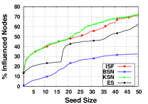
(a) Overlap = 0 (Scale-free, $\mathscr{H}_{0}$)

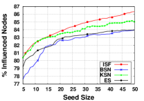
(b) Overlap = 500 (Scale-free, $\mathscr{H}_{500}$)

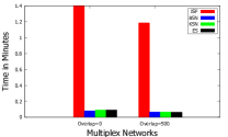
(c) Scale-free, $\mathscr{H}$

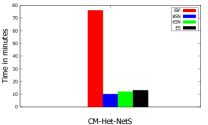
(d) CM-Het-NetS

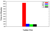
(e) Twitter-FSQ

Figure 6: (a), (b) Comparison of the four methods with no overlap and 500 overlapping users, respectively, in the scale-free multiplex setting. (c)–(e) Running time comparison for the four algorithms on different multiplexes.

IV-B1 Algorithm performance on synthesized multiplex networks

The performance of all four algorithms on the scale-free multiplex $\mathscr{H}_{0}$ with no overlapping users is shown in Fig. 6(a). As may be suggested by the analysis of the performance ratio for KSN, which depends on the number of overlapping users $o=0$, the performance of KSN equals or exceeds ISF. ES, where seeds are split evenly among the three layers, requires 40 seed users to get comparable activation to KSN and ISF at 20 seed users. BSN does the worst since it is choosing seed users from a single layer – since all three layers have 1000 nodes, BSN cannot activate more than $33\%$ of the multiplex, which it approaches as the number of seed nodes $l\geq 35$.

Next, we considered the $\mathscr{H}_{500}$, the multiplex with the same layers but 500 overlapping users, which is 1/6 of the original 3000 users. The performance is shown in Fig. 6(b). In the case of this significant overlap, ISF outperforms KSN. BSN is no longer limited to activation of at most $33\%$ and performs similarly to ES.

These results on the synthesized scale-free multiplex demonstrate how, in the case of small overlap we expect KSN to perform as well or better than ISF; however, as overlap increases, the performance of KSN will degrade with respect to ISF, a statement that we have demonstrated theoretically in section III-B1.

IV-B2 Running time

In Fig. 6(c), we compare the running time for the four algorithms on $\mathscr{H}_{0}$ and $\mathscr{H}_{500}$. The effect of parallelization by layer of the multiplex on the running time may be seen; note that for KSN, BSN, and ES, we are using CELF++ on each layer. This algorithm could be replaced by a more efficient single layer algorithm, which would further improve running time as compared to ISF.

IV-B3 Role of overlapping users

On total activation

To investigate the role of overlapping users further, we varied the number of overlapping users from 50 to 400 in the ER multiplex setting. The effect of this on the total activation of ISF can be seen in Fig 7(a). Increasing the number of overlapping users increases the number of influenced users.

On performance of KSN

We have already noticed, both from theoretical and experimental standpoints, that the performance of KSN with respect to the optimal solution is expected to degrade as the number of overlapping users increases. In this section, we examine how the performance of KSN compares with itself on the scale-free synthesized multiplexes as the number of overlapping users increases. The results are shown in Fig. 7(b). As the number of overlapping users increases, the algorithm’s performance improves drastically, demonstrating the efficacy of KSN even when overlapping users exist. With the overlapping percentage at 16.67%, KSN activates over 80% of the nodes in the multiplex with just five seed nodes, as opposed to in the case of no overlap, where activation is at roughly 35% with 5 seed nodes. In addition, this experiment provides further evidence of the strong benefit overlapping users provide in the influence propagation.

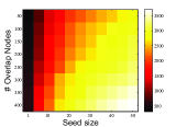
(a) Total activation of ISF: Overlap Size vs Seed Size (Erdos-Renyi)

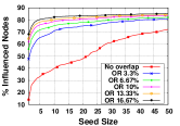
(b) Effect of overlapping on KSN performance (Scale-free)

Figure 7: Influence Spread for different overlap ratio, Diffusion Models- Net1: IC, Net2: LT

IV-C Algorithm performance on real networks

The first real multiplex we consider is based upon sections of Twitter and Foursquare (FSQ) networks. The generation of this dataset is described in [21]; overlapping users were identified by using Foursquare API v1 to identify the Twitter usernames corresponding to a Foursquare account. The weight of each link in Twitter is inferred by using frequency of tweets between users. In Foursquare, the weight of each link is assigned value 1, due to the lack of a message dataset. The number of overlapping nodes is 4100, see Table I.

The second real multiplex is based upon academic collaboration networks, described in [21]. The layers are organized by the research area: Condensed Matter (CM), High-Energy Theory (Het) [22], and Network Science (NetS) [23]. A user is considered to be overlapping if he or she has published in two or more of these three fields. The CM-HET-NetS (CHN) multiplex is considered an undirected network throughout the experiments. The number of overlapping users are 2860, 517, and 90 between CM-HET, CM-NetS, and HET-NetS, respectively; 75 users are present in all three networks.

IV-C1 Model selection

Saito et al. [13] have performed machine-learning techniques to match variants of the IC and LT models with real propagation events. They found that even on the same network, different propagation events may be better explained by disparate models. In all the Twitter-FSQ experiments we assigned Twitter the LT model, and Foursquare the IC model; experiments that swapped the model selection gave similar qualitative results. On CHN, we assigned CM, HET and NetS the LT, IC and LT models, respectively. Thresholds were assigned uniformly randomly in $[0,1]$, while edge weights were determined as described above for Twitter, and randomly in $[0,1]$ for the other networks. Notice that with this choice of models, Theorem 1 applies; therefore, the approximation ratios of ISF and KSN hold.

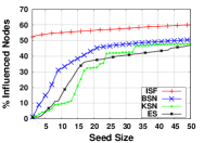
(a) Total activation in Twitter-FSQ

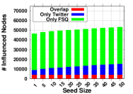
(b) Activated Node Composition (Twitter-FSQ)

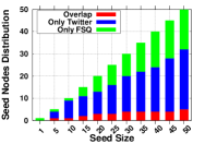
(c) Seed Node Composition (Twitter-FSQ)

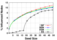
(d) Total activataion in CM-Het-NetS

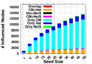
(e) Activated Node Composition (CHN)

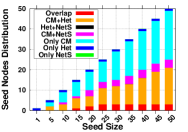
(f) Seed Node Composition (CHN)

Figure 8: Twitter-FSQ Network (top figures), co-author networks (bottom figures)

Networks	Nodes	Edges	Avg Deg
Twitter	48277	16304712	289.7
FSQ	44992	1664402	35.99
CM	40420	175692	8.69
Het	8360	15751	1.88
NetS	1588	2742	1.73

TABLE I: Traces of real networks

It is evident from Fig. 8(a) that the seeds found by ISF in Twitter-FSQ network outperforms BSN (20% larger for $l=50$) as well as ES and KSN. An interesting observation in this figure is that relatively few (overlapping) nodes are responsible for a lot of the propagation in the ISF case – the seed node composition is shown in Fig. 8(c). Also, in Fig. 8(b), we see influence spread is larger in FSQ compared to Twitter.

Since the Condensed Matter Network is comparatively larger than the other two, most of the seed users are selected from it as shown in Fig. 8(f). Therefore, a significant number of finally activated users also reside in this network. The influence spread obtained in the multiplex network only taking the seeds of BSN and KSN are very close to that obtained by the seed nodes identified by ISF. Nonetheless, ISF outperforms them as the seed set becomes larger, as shown in Fig. 8(d); this again illustrates the benefit of taking into account overlapping users in the solution.

As depicted in Fig. 8(b), the composition of influenced users in the Twitter-FSQ network suggests that majority of influenced users in the multiplex network belongs to FSQ which implies propagation spreads easily in this network compared to Twitter. The same observation can be drawn for CM network in case of co-author network, shown in Fig. 8(e). As illustrated in Fig. 8(c) and Fig. 8(f), the seed set of the multiplex network identified by ISF contains a much higher number of nodes from a specific network than other networks. In addition, overlapping users show significant role in diffusing information by occupying a considerable fraction of the seed set chosen by ISF.

Running time: In Fig. 6(e), we compare the running time for the four algorithms on CHN, and Twitter-FSQ multiplexes. The effect of parallelization by layer on the running time may be seen, with ISF taking much longer in all cases.

IV-D Scalability of KSN

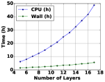
(a) $n_{ER}=10^{5}$

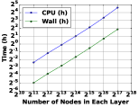
(b) $k=10$

Figure 9: Scalability of KSN

In our final set of experiments, we demonstrate the scalability of KSN on large multiplexes. For these experiments, we used synthesized multiplexes, where each layer is an ER network with average degree 5. Each layer has the same number $n_{ER}$ of vertices. Layer $i$ is assigned model IC if $i$ is even and model LT otherwise, with edge weights uniformly chosen in $(0,0.1)$. The number of overlapping users is set to $o=0.1n_{ER}$, and each overlapping user is present in all layers of the multiplex. For these experiments, the number of seeds $l=100$. Since the solution of IMM of size $m$ is not necessarily contained in the solution of size $m+1$, IMM is run on each layer for all values from 1 to $l$, as indicated in the pseudocode of KSN.

Results for the running time of KSN are shown in Fig. 9. The first experiment varies the number $k$ of layers in the multiplex from 5 to 17, with $n_{ER}=10^{5}$. Thus, the largest multiplex in this experiment has $1.54\times 10^{6}$ unique users. In Fig. 9(a), we show the running time in hours of KSN versus $k$, for both total CPU time and the wall-clock time. Thus, on the largest multiplex with $k=17$, KSN finished in roughly 5 hours of wall-clock time, demonstrating a high level of parallelization. Results for the second experiment are shown in Fig. 9(b), where the number of layers is fixed at $k=10$, and $n_{ER}$ is varied from 2048 to 131072. In this experiment, both the wall-clock time and CPU time increase linearly, with the wall-clock time below 4 hours on the largest multiplex with $1.19\times 10^{6}$ unique users.

V Related Works

In a seminal work on single-layer networks, Kempe et al. showed the IC and LT models were submodular [11] by utilizing a “live edge” approach, thereby allowing the use of a greedy algorithm to approximate the influence maximization on single networks. The “live edge” approach implicitly establishes the stronger GDS property as defined above for these models. The inapproximability of the classical max coverage problem precludes any better approximation to the influence maximization problem. Since this work, there have been a number of improvements to the running time of the greedy algorithm on single networks. The first improvement was through the use of priority queue to do a “lazy evaluation” of estimated influence in [24]. Cohen et al. provided an approximation algorithm for influence maximization one or two orders of magnitude faster than previous works on single-layer networks [5]; Kuhnle et al. [25] adapted this framework for the threshold activation problem. Borgs et al. provide a nearly runtime-optimal algorithm on single networks with the IC model [6], and Tang et al. [7] provided a fast algorithm with with high probability achieves the greedy ratio $1-1/e-\epsilon$ for the triggering model; this method was further improved by Tang [18] using martingales. Nguyen et al. [26, 27] and Huang et al. [28] have further improved the sampling techniques to yield even faster algorithms for the single-layer network problem with the $1-1/e-\epsilon$ ratio; also, Li et al. [29] have developed a scalable and nearly optimal algorithm.

A considerable number of works have studied influence maximization for variants of IC models and its extensions such as [4, 3]. For a deterministic variant of LT, Feng et al. [30] showed NP-completeness for the problem and Dinh et al [31] proved the inapproximability as well as proposed efficient algorithms for this problem on a special case of LT model. In their model, the influence between users is uniform and a user is influenced if a certain fraction $\rho$ of his friends are active.

Researchers have started to explore the influence maximization problem on multiplex networks with works of Yagan et al. [32] and Liu et al. [33] which studied the connection between offline and online networks. The first work investigated the outbreak of information using the SIR model on random networks. The second one analyzed networks formed by online interactions and offline events. The authors focused on understanding the flow of information and network clustering but not solving the heterogeneous influence problem.

Shen et al. [21] explored the information propagation in multiplex online social networks taking into account the interest and engagement of users. The authors combined all networks into one network by representing an overlapping user as a super node. This method cannot preserve the heterogeneity of the layers. Nguyen et al. [34] studied the influence maximization problem which handles multiple networks but only considers homogeneous diffusion process across all the networks. None of these works took into consideration the heterogeneity of diffusion processes in multiplex networks. On the other hand, our scheme overcomes these shortcomings by enabling different networks to have different influence propagation models. Pan et al. [35] study threshold activation problems on multiplex networks under a diffusion model with continuous time.

VI Conclusion

We formulate the Multiplex Influence Maximization problem that seeks to maximize influence propagation in a multiplex with overlapping users and heterogeneous propagation. We provide a property (GDS) which carries over from single layer to multiplex propagation, giving the $1-1/e$ ratio for the greedy algorithm ISF if it is satisfied on each layer. We also develope an approximation algorithm KSN that benefits from the optimizations that influence maximization in a single network has undergone (e.g. in [7, 6, 5]). We prove the approximation ratio of KSN, which depends on the number of overlapping users. As demonstrated in our experimental section, the performance KSN may fall short of ISF when overlapping effects become large. Due to the long running time of ISF, future work would include attempting to find faster approximation algorithms in the heterogeneous multiplex setting.

VII Acknowledgements

This work is supported in part by NSF grant CNS-1443905 and DTRA grant HDTRA1-14-1-0055.

References

- [1] 216 social media and internet statistics. http://thesocialskinny.com/216-social-media-and-internet-statistics-september-2012/.
- [2] Kazumi Saito, Masahiro Kimura, Kouzou Ohara, and Hiroshi Motoda. Selecting information diffusion models over social networks for behavioral analysis. In Machine Learning and Knowledge Discovery in Databases, Lecture Notes in Computer Science, volume 6323, pages 180–195. 2010.
- [3] David Kempe, Jon Kleinberg, and Éva Tardos. Influential nodes in a diffusion model for social networks. In ICALP, 2005.
- [4] Wei Chen, Chi Wang, and Yajun Wang. Scalable influence maximization for prevalent viral marketing in large-scale social networks. In KDD, 2010.
- [5] Edith Cohen, Daniel Delling, Thomas Pajor, and Renato F Werneck. Sketch-based influence maximization and computation: Scaling up with guarantees. In Proceedings of the 23rd ACM International Conference on Conference on Information and Knowledge Management, pages 629–638. 2014.
- [6] Christian Borgs, Michael Brautbar, Jennifer Chayes, and Brendan Lucier. Maximizing social influence in nearly optimal time. In Proceedings of the Twenty-Fifth Annual ACM-SIAM Symposium on Discrete Algorithms, SODA ’14, pages 946–957. SIAM, 2014.
- [7] Youze Tang, Xiaokui Xiao, and Yanchen Shi. Influence maximization: Near-optimal time complexity meets practical efficiency. In Proceedings of the 2014 ACM SIGMOD International Conference on Management of Data, SIGMOD ’14, pages 75–86. ACM, New York, NY, USA, 2014.
- [8] Overlap among major social network services. http://www.tomhcanderson.com/2009/07/09/overlap-among-major-social-network-services/.
- [9] Tereza Iofciu, Peter Fankhauser, Fabian Abel, and Kerstin Bischoff. Identifying users across social tagging systems. In ICWSM, 2011.
- [10] Francesco Buccafurri, Gianluca Lax, Antonino Nocera, and Domenico Ursino. Discovering links among social networks. In ECML PKDD. 2012.
- [11] David Kempe, Jon Kleinberg, and Éva Tardos. Maximizing the spread of influence through a social network. In KDD, 2003.
- [12] G. Nemhauser, L. Wolsey, and M. Fisher. An analysis of the approximations for maximizing submodular set functions. In Mathematical Programming, volume 14, pages 265–294. 1978.
- [13] Kazumi Saito, Masahiro Kimura, Kouzou Ohara, and Hiroshi Motoda. Selecting information diffusion models over social networks for behavioral analysis. In Machine Learning and Knowledge Discovery in Databases, pages 180–195. Springer, 2010.
- [14] W. Chen, L.V.S. Lakshmanan, and C. Castillo. Information and influence propagation in social networks. In Synthesis Lectures on Data Management. 2013.
- [15] Hui Li, Sourav S Bhowmick, Aixin Sun, and Jiangtao Cui. Conformity-aware influence maximization in online social networks. The VLDB Journal, 24(1):117–141, 2015.
- [16] Amit Goyal, Wei Lu, and Laks VS Lakshmanan. Celf++: optimizing the greedy algorithm for influence maximization in social networks. In Proceedings of the 20th international conference companion on World wide web, pages 47–48. ACM, 2011.
- [17] Ashok K. Chandra, D.S. Hirschberg, and C.K. Wong. Approximate algorithms for some generalized knapsack problems. In Theoretical Computer Science, volume 3, pages 293–304. 1976.
- [18] Youze Tang. Influence Maximization in Near-Linear Time : A Martingale Approach. In Proceedings of the 2015 ACM SIGMOD International Conference on Management of Data, pages 1539–1554, 2015.
- [19] Albert-László Barabási and Réka Albert. Emergence of scaling in random networks. volume 286, pages 509–512. American Association for the Advancement of Science, 1999.
- [20] Ning Chen. On the approximability of influence in social networks. In SODA, 2008.
- [21] Yilin Shen, Thang N. Dinh, Huiyuan Zhang, and My T. Thai. Interest-matching information propagation in multiple online social networks. In CIKM, 2012.
- [22] Mark EJ Newman. The structure of scientific collaboration networks. PNAS, 98(2):404–409, 2001.
- [23] M. E. J. Newman. Finding community structure in networks using the eigenvectors of matrices. Phys. Rev. E, 74:036104, 2006.
- [24] J. Leskovec, A. Krause, and C. Guestrin. Cost-effective outbreak detection in networks. In KDD. 2007.
- [25] Alan Kuhnle, Tianyi Pan, Md A Alim, and My T Thai. Scalable Bicriteria Algorithms for the Threshold Activation Problem in Online Social Networks. In IEEE International Conference on Computer Communications, 2017.
- [26] H. T. Nguyen, T. N. Dinh, and M. T. Thai. Cost-aware Targeted Viral Marketing in Billion-scale Networks.
- [27] H.T. Nguyen, M. T. Thai, and T. N. Dinh. Stop-and-Stare: Optimal Sampling Algorithms for Viral Marketing in Billion-Scale Networks. In ACM SIGMOD/POSD Conference, 2016.
- [28] Keke Huang, Sibo Wang, Glenn Bevilacqua, Xiaokui Xiao, and Laks V S Lakshmanan. Revisiting the Stop-and-Stare Algorithms for Influence Maximization. Proceedings of the VLDB Endowment, 10(9):913–924, 2017.
- [29] Xiang Li, J. David Smith, Thang N. Dinh, and My T. Thai. Why approximate when you can get the exact? Optimal Targeted Viral Marketing at Scale. In IEEE International Conference on Computer Communications, 2017.
- [30] Feng Zou, Zhao Zhang, and Weili Wu. Latency-bounded minimum influential node selection in social networks. In WASA, 2009.
- [31] Thang N. Dinh, Dung T. Nguyen, and My T. Thai. Cheap, easy, and massively effective viral marketing in social networks: truth or fiction? In Proceedings of the 23rd ACM conference on Hypertext and social media, HT ’12, 2012.
- [32] Osman Yagan, Dajun Qian, Junshan Zhang, and Douglas Cochran. Information diffusion in overlaying social-physical networks. In CISS, 2012.
- [33] Xingjie Liu, Qi He, Yuanyuan Tian, Wang-Chien Lee, John McPherson, and Jiawei Han. Event-based social networks: linking the online and offline social worlds. In KDD, 2012.
- [34] Dung T. Nguyen, Huiyuan Zhang, Soham Das, My T. Thai, and Thang N. Dinh. Least cost influence in multiplex social networks: Model representation and analysis. In ICDM, 2013.
- [35] Tianyi Pan, Alan Kuhnle, Xiang Li, and My T. Thai. Popular Topics Spread Faster: New Dimension for Influence Propagation in Online Social Networks. In International Conference on Data Mining (ICDM), pages 1–11, 2017.