Corner transport upwind lattice Boltzmann model for bubble cavitation

Abstract

Aiming to study the bubble cavitation problem in quiescent and sheared liquids, a third-order isothermal lattice Boltzmann (LB) model that describes a two-dimensional ($2D$) fluid obeying the van der Waals equation of state, is introduced. The evolution equations for the distribution functions in this off-lattice model with 16 velocities are solved using the corner transport upwind (CTU) numerical scheme on large square lattices (up to $6144\times 6144$ nodes). The numerical viscosity and the regularization of the model are discussed for first and second order CTU schemes finding that the latter choice allows to obtain a very accurate phase diagram of a nonideal fluid. In a quiescent liquid, the present model allows to recover the solution of the $2D$ Rayleigh-Plesset equation for a growing vapor bubble. In a sheared liquid, we investigated the evolution of the total bubble area, the bubble deformation and the bubble tilt angle, for various values of the shear rate. A linear relation between the dimensionless deformation coefficient $D$ and the capillary number $Ca$ is found at small $Ca$ but with a different factor than in equilibrium liquids. A non-linear regime is observed for $Ca\gtrsim 0.2$.

I Introduction

The cavitation and growth of bubbles in stretched or superheated liquids is a phenomenon frequently appearing in nature with relevant scientific and technical interest rallison-1984 . Cavitation is a sudden transition from liquid to vapor that can be promoted by the decrease of the pressure in a stretched liquid below the liquid’s vapor pressure as well as by the nucleation of bubbles in a superheated liquid brennen-1995 . Examples of these processes, among others, are given by the cavitation corrosion of materials exposed to water plesset-1963 , phase changes in cosmology devega-2001 , vulcanism massol-2005 . In the following we will be interested in studying numerically the kinetics and dynamics of a single vapor bubble which cavitates in a superheated liquid which is either at rest or subject to shear. Previous studies of a nucleating bubble are very limited and rely on Molecular Dynamics kuksin-2010 ; watanabe-2010 ; diemand-2014 ; angelil-2014 , lattice Boltzmann (LB) simulations sukop-2005 ; chen-2010 ; chen-2011 ; zhong-2012 , and other numerical methods feng-1997 . Growth curves of the bubble in a quiescent fluid were obtained in Refs. angelil-2014 ; chen-2010 ; chen-2011 and compared to the Rayleigh-Plesset (RP) growth model rayleigh-1917 ; plesset-1949 ; plesset-1977 . Very first attempts of addressing the cavitation study in a sheared liquid were presented in Refs. chen-2010 ; chen-2011 .

From more than two decades, the use of LB models for phase-separating fluids is widely expanding because of the parallel nature of their basic algorithm, as well as for their capability to easily handle interactions chen_annurev1998 ; succi_2001 ; sukop_2006 ; aidun_annurev2010 ; guo2013 ; sukop2015 ; krueger2017 . A characteristic feature of the LB models is the polynomial expansion of the equilibrium single-particle distribution function up to a certain order $N$ with respect to the fluid particle velocity. This expansion is made by projecting the equilibrium distribution function on a set of orthogonal polynomials, e.g., the Hermite polynomials shan_jfm2006 . In the widely used collision-streaming LB models, the velocity space is discretized so that the velocity vectors of the fluid particles leaving a node of the lattice are oriented towards the neighboring nodes cao1997 . Such models are also called on-lattice models.

In this paper we perform a qualitative and quantitative analysis of the bubble cavitation problem using a third-order isothermal LB model that describes a two-dimensional (2D) nonideal fluid obeying the van der Waals equation of state (EOS) dsfd2014 . Though several equations of state exist yuan2006 and different lattice Boltzmann models are available to handle high liquid-vapor density ratios chen2014 , the used EOS is a well-established and classic benchmark fitting our goal. Indeed, a recent numerical study kaehler-2015 , based on the van der Waals EOS, allowed to elucidate qualitatively and quantitatively the cavitation inception at a sack-wall obstacle in a 2D geometry. The study of two-dimensional bubbles has attracted a lot of interest in the past. Indeed, an immiscible drop in shear flow has been studied theoretically rich1968 ; buck1973 and numerically hall1996 ; hall21996 . For two-dimensional miscible binary mixtures the problem of bubble break-up and dissolution under shear was also addressed wagner1997 .

The $2D$ LB model used in this paper, which is described in Sections II A-C, has 16 off-lattice velocities and is based on the Gauss-Hermite quadrature method dsfd2014 ; shan_jfm2006 . In Ref.dsfd2014 , the evolution equations for the distribution functions in the LB model were solved using the first order corner transport upwind (CTU1) numerical scheme dsfd2014 ; colella1990 ; leveque1996 ; leveque2002 ; trangenstein2009 . Besides the capability of handling off-lattice velocity sets in LB models, this very simple scheme, which is of first order with respect to the lattice spacing $\delta s$, involves only four neighboring lattice nodes and is easily parallelizable, like the collision-streaming scheme. Despite of these advantages, the computer simulations performed with the CTU1 scheme are plagued by its numerical viscosity, as discussed in Section II.4 below. To improve the accuracy of our simulations, in this paper we further extended the previous LB model dsfd2014 by incorporating the second-order corner transport upwind scheme (CTU2) leveque1996 ; leveque2002 ; trangenstein2009 . These schemes, though well documented in the mathematical literature for the numerical solution of hyperbolic partial differential equations, are here demonstrated to have the capabilities to deal with an off-lattice discrete velocity set in a LB model, and the provided results are encouraging.

In order to follow the bubble evolution on large lattices during long time intervals, we implemented this model on NVIDIA^® graphics processing units (M2090 and K40). The resulted code was first tested by simulating the evolution of shear waves oriented along the horizontal axis or along the diagonal of a square lattice. During these simulations, we checked for anisotropic effects in the LB model and we found that no regularization procedure is needed for small values of the relaxation time ($\tau\leq 0.1$), i.e., when the isothermal fluid is not too far from equilibrium and obeys the mass and momentum conservation equations (Section II.4). Further tests reported in Section II.5 refer to the liquid-vapor phase diagram and to the effect of both the relaxation time $\tau$ and the lattice spacing $\delta s$ on the accuracy of the liquid and vapor density values obtained by equilibrating a plane interface.

Since the growth or shrinkage of a bubble mainly depends on its initial size at fixed temperature and pressure, in Section III.1 we checked the theoretical prediction laurila-2012 of the critical radius of the bubble neither growing nor shrinking in a quiescent superheated liquid. In such a system the bubble Helmholtz free energy density can decrease by increasing the bubble size via evaporation of some of the surrounding liquid to the coexistence densities. Alternatively, the interfacial free energy increases as the bubble shrinks. The competition between these two mechanisms, under the constraint of local mass conservation, induces either the growth or the collapse of the bubble.

When the bubble cavitates, the time evolution of its radius can be theoretically described by the RP model rayleigh-1917 ; plesset-1949 ; plesset-1977 , where the Navier-Stokes equation is re-written for a spherical bubble in an infinite liquid domain. In Section III.2 of this paper we derive the RP equation in two dimensions and compare our numerical findings to its predictions. This will allow to test the accuracy of the present off-lattice numerical model in addressing the problem of cavitation. Indeed, the RP equation is useful to quantitatively characterize the growth of bubbles in cavitation. This problem is often tackled in two dimensions due to its heavy computational cost falcucci-2013 ; kaehler-2015 . In this way the analysis of the RP equation in a low dimensionality system may give an analytical support to further numerical studies. Our study shows that the numerical model gives the right growth rate of a cavitating bubble up to a final bubble size which is more than one order of magnitude larger than its initial value.

Finally, despite the deep scientific and technological interest for the problem of the deformation of a bubble in an immiscible fluid under an external flow rallison-1984 , the growth of a vapor bubble in shear flow has not been the subject of extended investigation. In the present study we are able to characterize the growth and the deformation of the bubble on time scales long enough to access non-negligible values of the capillary number (Section III.3). Moreover, the tilt angle of the deformed bubble with respect to the flow direction and its areal extension are computed.

In this paper, all physical quantities are nondimensionalized by using the following reference quantities pre2004 : the fluid particle number density $n_{R}=N_{A}/V_{mc}$, the critical temperature $T_{R}=T_{c}$, the fluid particle mass $m_{R}=M/N_{A}$, the length $l_{R}=1/\sqrt[3]{n_{R}}$, the speed $c_{R}=\sqrt{k_{B}T_{R}/m_{R}}$, and the time $t_{R}=l_{R}/c_{R}$. Here $N_{A}$ is Avogadro’s number, $V_{mc}$ is the molar volume at the critical point, $T_{c}$ is the critical temperature and $M$ is the molar mass.

II Description of the model

II.1 Velocity set, single-particle distribution functions and evolution equations

In order to derive the Navier-Stokes equations from the Boltzmann equation in the case of a compressible isothermal fluid shan_jfm2006 ; ambrus_pre2012 ; ambrus_jcph2016 , the moments up to the order $N=3$ of the Maxwell - Boltzmann equilibrium single-particle distribution function

$$f^{eq}\equiv f^{eq}({\bm{x}},{\bm{\xi}},t)=\frac{\rho}{\,(2\pi T)^{D/2}\,}\exp\left[-\frac{\,\,({\bm{\xi}}-{\bm{u}})^{2}\,}{2T}\right]$$ (1)

are required according to the Chapman-Enskog method chen_annurev1998 ; succi_2001 ; sukop_2006 ; aidun_annurev2010 ; guo2013 ; sukop2015 ; krueger2017 . In Eq. (1) above, ${\bm{x}}$ is the fluid particle position vector, ${\bm{\xi}}$ is the fluid particle velocity vector, $t$ is the time and $\rho\equiv\rho({\bm{x}},t)$, $T\equiv T({\bm{x}},t)$, ${\bm{u}}\equiv{\bm{u}}({\bm{x}},t)$ are the local values of the fluid particle number density, fluid temperature and fluid velocity, respectively. In the Gauss - Hermite LB model of order $N$ in $D$ dimensions (see shan_jfm2006 and references therein), the equilibrium single-particle distribution function (1) is expanded up to order $N$ with respect to the tensor Hermite polynomials ${\bm{\mathcal{H}}}^{(\ell)}({\bm{\xi}})\equiv{\bm{\mathcal{H}}}^{(\ell)}_{\alpha_{1}\ldots\alpha_{\ell}}({\bm{\xi}})$,  $0\leq\ell\leq N$ ($1\leq\alpha_{1},\,\ldots\alpha_{l}\leq D$) :

$$f^{eq}({\bm{x}},{\bm{\xi}},t)\,=\,\omega({\bm{\xi}})\,\sum_{\ell=0}^{N}\,\frac{1}{\ell!}\,{\bm{a}}^{eq,(\ell)}_{\alpha_{1}\ldots\alpha_{\ell}}({\bm{x}},t)\,{\bm{\mathcal{H}}}^{(\ell)}_{\alpha_{1}\ldots\alpha_{\ell}}({\bm{\xi}})$$ (2)

where summation over repeated lower Greek indices is implicitly understood and

$$\omega({\bm{\xi}}) = \frac{1}{\,2\pi\,}\,e^{-{\bm{\xi}}^{2}/2T}$$

$${\bm{a}}^{eq,(\ell)}_{\alpha_{1}\ldots\alpha_{\ell}}({\bm{x}},t) = \int f^{eq}({\bm{x}},{\bm{\xi}},t){\bm{\mathcal{H}}}^{(\ell)}_{\alpha_{1}\ldots\alpha_{\ell}}({\bm{\xi}})d{\bm{\xi}}.\rule{0.0pt}{22.76219pt}$$ (3)

All the moments up to order $N$ of $f^{eq}({\bm{x}},{\bm{\xi}},t)$, namely $\int f^{eq}({\bm{x}},{\bm{\xi}},t)\xi_{\alpha_{1}}\ldots\xi_{\alpha_{N}}d{\bm{\xi}}$, are thereafter recovered using appropriate quadrature methods in the velocity space shan_jfm2006 ; ambrus_pre2012 ; ambrus_jcph2016 ; shan_prl1998 ; piaud_ijmpc2014 .

The Gauss-Hermite quadrature method shan_jfm2006 ; hildebrandt ; shizgal allows one to get a finite set of velocity vectors (quadrature points) ${\bm{\xi}}_{k}$, $k=1,\,2,\,\ldots\,K$, as well as their associated weights $w_{k}$. The expansion (2), followed by the application of the Gauss-Hermite quadrature method leads to the LB model, where the Boltzmann equation is replaced by a set of evolution equations for the functions $f_{k}\equiv f_{k}({\bm{x}},t)=f({\bm{x}},{\bm{\xi}}_{k},t)$, which are usually defined in the nodes ${\bm{x}}$ of a regular lattice. When using the BGK collision term in a $D$-dimensional LB model of order $N$ shan_jfm2006 ; chen_annurev1998 ; succi_2001 ; sukop_2006 ; ambrus_jcph2016 ; shan2008 , the functions $f_{k}$, $1\leq k\leq K=(N+1)^{D}$, evolve according to

$$\partial_{t}f_{k}\,+\,\xi_{k,\gamma}\,\partial_{\gamma}f_{k}\,=\,-\,\frac{1}{\,\tau\,}\,\left[\,f_{k}\,-\,f^{eq}_{k}\,\right]\,+\,F_{k}\qquad,\qquad 1\leq k\leq K$$ (4)

where $\partial_{t}=\partial/\partial_{t}$,  $\xi_{k,\gamma}$, $\gamma\in\{x,y,\ldots\}$, are the Cartesian components of the velocity vector ${\bm{\xi}}_{k}$, $\partial_{\gamma}=\partial/\partial_{x_{\gamma}}$,

$$f_{k}^{eq}\equiv f_{k}^{eq}({\bm{x}},t)\,=\,w_{k}\,\sum_{\ell=0}^{N}\,\frac{1}{\ell!}\,{\bm{a}}^{eq,(\ell)}_{\alpha_{1}\ldots\alpha_{\ell}}({\bm{x}},t)\,{\bm{\mathcal{H}}}^{(\ell)}_{\alpha_{1}\ldots\alpha_{\ell}}({\bm{\xi}}_{k}),$$ (5)

and $\tau$ is the relaxation time. In the Gauss - Hermite LB model of order $N=3$, the expressions of the functions $f_{k}^{eq}\equiv f_{k}^{eq}({\bm{x}},t)$ and of the force term $F_{k}$ are shan_jfm2006 ; niu2007pre ; suga2010pre ; suga2013fdr :

$$f^{eq}_{k} = w_{k}\rho\left\{\,1\,+\,{\bm{\xi}}_{k}\cdot{\bm{u}}\,+\,\frac{1}{\,2\,}\left[({\bm{\xi}}_{k}\cdot{\bm{u}})^{2}\,-\,u^{2}\,+\,(T-1)(\bm{\xi}^{2}_{k}-2)\right]\right.$$ (6)

$$+ \left.\frac{\,{\bm{\xi}}_{k}\cdot{\bm{u}}\,}{6}\,\left[({\bm{\xi}}_{k}\cdot{\bm{u}})^{2}-3u^{2}\,+\,3(T-1)(\bm{\xi}^{2}_{k}-4)\right]\right\}\rule{0.0pt}{25.60747pt}$$

$$F_{k} = w_{k}\rho\left\{\,{\bm{\xi}}_{k}\cdot{\bm{g}}\,+\,({\bm{\xi}}_{k}\cdot{\bm{g}})({\bm{\xi}}_{k}\cdot{\bm{u}})\,-\,{\bm{g}}\cdot{\bm{u}}\,+\,\frac{1}{\,2\rho\,}{\bm{a}}^{(2)}\left[\,({\bm{\xi}}_{k}\cdot{\bm{g}}){\bm{\mathcal{H}}}^{(2)}({\bm{\xi}}_{k})\,-\,2{\bm{g}}{\bm{\xi}}_{k}\right]\right\}$$ (7)

where

$$\rho\equiv\rho({\bm{x}},t) = \sum_{k=1}^{K}f_{k}\,=\,\sum_{k=1}^{K}f_{k}^{eq}$$ (8)

$${\bm{u}}\equiv{\bm{u}}({\bm{x}},t) = \frac{1}{\,\rho\,}\sum_{k=1}^{K}f_{k}{\bm{\xi}}_{k}\,=\,\frac{1}{\,\rho\,}\sum_{k=1}^{K}f_{k}^{eq}{\bm{\xi}}_{k}\rule{0.0pt}{25.60747pt}$$ (9)

are the local density and velocity. In the expression (7) of $F_{k}$, ${\bm{g}}$ is an acceleration depending on the specific problem that is investigated with the LB model. For the model used in this paper, ${\bm{g}}$ is given in Eq. (10) below.

Table 1: The Cartesian projections of the vectors ${\bm{\xi}}_{k}$,  $k=1,\,2,\,\ldots K=16$, and their corresponding weights $w_{k}$ used in the two-dimensional isothermal LB model of order $N=3$ shan_jfm2006 ; dsfd2014 .

$k$	$\xi_{k,x}$	$\xi_{k,y}$	$w_{k}$
1 …4	$\pm\sqrt{3-\sqrt{6}}$	$\pm\sqrt{3-\sqrt{6}}$	$(5+2\sqrt{6})/48$
5 …8	$\pm\sqrt{3+\sqrt{6}}$	$\pm\sqrt{3-\sqrt{6}}$	$1/48$
9 …12	$\pm\sqrt{3-\sqrt{6}}$	$\pm\sqrt{3+\sqrt{6}}$	$1/48$
13 …16	$\pm\sqrt{3+\sqrt{6}}$	$\pm\sqrt{3+\sqrt{6}}$	$(5-2\sqrt{6})/48$

All simulations reported in this paper were performed with a two-dimensional ($D=2$) LB model of order $N=3$ using a constant value of the fluid temperature $T$. For convenience, in Table 1 we provide the Cartesian projections of the $16$ velocity vectors ${\bm{\xi}}_{k}$ used in this model, as well as their associated weights $w_{k}$ shan_jfm2006 ; dsfd2014 . More than a decade ago, this $16$ velocity set was used also in entropic LB models ansumali_epl2003 ; bardow_epl2006 ; bardow_pre2008 .

II.2 Force term

The following expression of the acceleration ${\bm{g}}$ is used in order to simulate the evolution of a van der Waals fluid where the surface tension is controlled by the parameter $\kappa$ chen_annurev1998 ; succi_2001 ; sukop_2006 ; dsfd2014 ; pre2004 ; cicp2010 ; luo1998prl ; luo2000 ; coclite :

$${\bm{g}}\,=\,\frac{1}{\,\rho\,}\,{\bm{\nabla}}(p^{i}\,-\,p^{w})\,+\,\kappa{\bm{\nabla}}(\Delta\rho)$$ (10)

where $p^{i}=\rho T$ is the ideal gas pressure and $p^{w}$ is the van der Waals pressure given in Eq. (14) below. The equilibrium properties of the fluid can be described by the Helmholtz free-energy functional rowl

$$\Psi=\int d{\bf x}\Big{[}\psi(\rho,T)+\frac{\kappa}{2}(\nabla\rho)^{2}\Big{]}$$ (11)

where the bulk free-energy density is

$$\psi=\rho T\ln\Big{(}\frac{3\rho}{3-\rho}\Big{)}-\frac{9}{8}\rho^{2}.$$ (12)

The pressure tensor ${\bm{\Pi}}$ evans can be computed from Eq. (11)

$${\bm{\Pi}}=\Big{[}p^{w}-\kappa\rho\Delta\rho-\frac{\kappa}{2}(\nabla\rho)^{2}\Big{]}{\bm{1}}+\kappa{\bm{\nabla}}\rho{\bm{\nabla}}\rho$$ (13)

Here ${\bm{1}}$ is the unit tensor and

$$p^{w}=\rho\frac{\partial\psi}{\partial\rho}-\psi=\frac{3\rho T}{3-\rho}-\frac{9}{8}\,\rho^{2}$$ (14)

is the non-dimensionalized van der Waals equation of state with the critical point at $\rho_{c}=1$, $T_{c}=1$. The acceleration ${\bf g}$ is then related to the pressure tensor by the relationship

$$\rho{\bm{g}}={\bm{\nabla}}p^{i}-{\bm{\nabla}}\cdot{\bm{\Pi}}.$$ (15)

In the presence of the force term $F_{k}$ given by Eq. (7), the conservation equations for mass and momentum, as derived from (4) using the Chapman-Enskog procedure, are klimontovich ; pre2004 ; cicp2010 ; noitermico

$$\partial_{t}\rho+\nabla(\rho{\bm{u}}) = 0$$ (16)

$$\partial_{t}(\rho{\bm{u}})+\nabla(\rho{\bm{u}}{\bm{u}}) = -\nabla\cdot\left[\bm{\Pi}-{\bm{S}}\right]\rule{0.0pt}{19.91692pt}$$ (17)

where the components of the viscous stress tensor ${\bm{S}}$ are

$$S_{\alpha\beta}=\rho T\tau\,\left[\partial_{\alpha}u_{\beta}+\partial_{\beta}u_{\alpha}-(\nabla\cdot{\bm{u}})\delta_{\alpha\beta}\right].$$ (18)

Unlike the LB models of order $N=2$, the term $(\nabla\cdot{\bm{u}})\delta_{\alpha\beta}$ of the viscous stress tensor in Eq. (18), is no longer neglected in the present model and no spurious terms appear.

The use of large stencils in order to compute the space derivatives of the pressure difference $(p^{i}\,-\,p^{w})$ and the local fluid density $\rho$, which appear in Eq. (10), is known to improve the isotropy of the phase interface, as well as the accuracy of the values of the coexistence densities in the phase diagram shan2008 ; leclaire ; kart ; mattila2014 ; siebert2014 ; dsfd2014 . In this paper, we used a 25 point stencil to compute the values of ${\bm{\nabla}}(p^{i}\,-\,p^{w})$ and $\kappa{\bm{\nabla}}(\Delta\rho)$. The procedure is documented in Refs.dsfd2014 ; leclaire ; kart ; mattila2014 ; siebert2014 and can be easily implemented on Graphics Processing Units (GPUs) using the shared memory facility farber ; cook ; professionalCUDA ; cudaguide .

II.3 Corner transport upwind schemes

II.3.1 First order corner transport upwind

The $16$ velocity vectors ${\bm{\xi}}_{k}$, whose Cartesian projections are shown in Table 1, are off-lattice vectors, i.e., vectors that do not point from one node of the square lattice to another one. For this reason, the collision - streaming scheme chen_annurev1998 ; succi_2001 ; sukop_2006 ; aidun_annurev2010 cannot be used in this case. Alternative schemes like the interpolation supplemented LB schemes, the Runge-Kutta time-marching schemes associated with various space-discretization methods, or the elaborate characteristics-based off-lattice LB schemes yuan2006 ; ansumali_epl2003 ; bardow_epl2006 ; bardow_pre2008 ; deville ; philippi_pre2006 ; siebert_pre2008 ; surmas_eurJph2009 ; chika_pre2009 ; ansumali_pre2008 ; ansumali_pre2010 ; islb1997 ; islb2004 ; jcph2009 ; ubertini_ccph2008 ; guo_pre2003 ; lee_jcph2001 ; lee_jcph2003 ; hejranfar_pre2015 are computationally expensive and difficult to stabilize, besides requiring specific treatment of the force and the advection terms in the evolution equations (4).

The first order corner transport upwind (CTU1) scheme was introduced more than two decades ago in the mathematical literature related to hyperbolic equations colella1990 ; leveque1996 ; leveque2002 ; trangenstein2009 . Although this scheme is simple enough and very convenient for solving the LB evolution equations (4) on square or cubic lattices, regardless of the orientation of the velocity vectors ${\bm{\xi}}_{k}$, its application to LB models was not considered in the literature until recently dsfd2014 ; australia2014 . Other finite-volume schemes, mainly developed for non-uniform meshes, were already used in the so-called volumetric lattice Boltzmann models nannelli1992 ; hchen_pre1998 ; rzhang_pre2001 ; mauro_pre2010 .

The evolution of $f_{k}\equiv f_{k}({\mathbf{x}},t)$ is governed by Eqs. (4), which form a system of hyperbolic equations with non vanishing source terms. A simple way to solve hyperbolic equations with source terms is to split them into two steps, which can be treated explicitly leveque2002 . The first step refers to the advection process, i.e., the left hand side of Eq. (4), while the second one refers to its right hand side, which includes the collision term as well as the force term. Let us consider the lattice cell centered in the node ${\mathbf{x}}=(x,y)$ of a $2D$ square lattice with $L_{x}\times L_{y}$ nodes. For convenience, we introduce the notation $f_{k,i,j}^{n}\equiv f_{k}(x=i\delta s,y=j\delta s,t=n\delta t)$, where $\delta s$ is the lattice spacing, $0\leq i<L_{x}$, $0\leq j<L_{y}$, $\delta t$ is the time step and $n=0,\,1,\,2,\,\ldots\infty$. When using the CTU1 scheme to account for the advection process, the Courant-Friedrichs-Levy (CFL) condition trangenstein2009

$${\mathrm{max}}_{k}\,\left\{\,|\xi_{k,x}|\delta t\,,\,|\xi_{k,y}|\delta t\,\right\}\,\leq\,\delta s$$ (19)

ensures that the new value $f_{k,i,j}^{n+1}$ receives contributions from at most four neighboring nodes, according to dsfd2014 ; trangenstein2009 ; australia2014

$$f_{k,i,j}^{n+1}\,=\, \frac{{\displaystyle{1}}}{\,{\displaystyle{(\delta s)^{2}}}\,\rule{0.0pt}{11.38109pt}} \left[\rule{0.0pt}{11.38109pt}\,{{f_{k,i,j}^{n}\,(\delta s-|\xi_{k,x}|\delta t)\,(\delta s-|\xi_{k,y}|\delta t)}}\,+\,f_{k,i-\varsigma_{k,x},j}^{n}\,|\xi_{k,x}|\,(\delta s-|\xi_{k,y}|\delta t)\,\delta t\,\right.$$ (20)

$$+ \left.\,f_{k,i,j-\varsigma_{k,y}}^{n}\,|\xi_{k,y}|\,(\delta s-|\xi_{k,x}|\delta t)\,\delta t\,+\,f_{k,i-\varsigma_{k,x},j-\varsigma_{k,y}}^{n}\,|\xi_{k,x}|\,|\xi_{k,y}|\,(\delta t)^{2}\,\rule{0.0pt}{11.38109pt}\right]\rule{0.0pt}{22.76219pt}$$

In the equation above, the symbol $\varsigma_{k,\alpha}$, $1\leq k\leq K$, $\alpha\in\{x,y\}$, is defined as follows:

$$\varsigma_{k,\alpha}=\left\{\begin{array}[]{rcl}1&,&\xi_{k,\alpha}\geq 0\\ -1&,&\xi_{k,\alpha}<0.\end{array}\right.$$ (21)

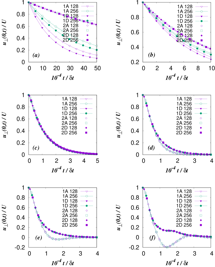
Figure 1: Evolution of the normalized peak velocity $u_{\perp}(0,t)/U$ of decaying shear waves without regularization, for various values of the relaxation time $\tau=$ 0.001 (a), 0.010 (b), 0.100 (c), 0.200 (d), 0.300 (e), 0.500 (f). The results obtained using the CTU$n$ scheme, $n\in\{1,2\}$, and the lattice spacing $\delta s=1/S$, $S\in\{128,256\}$, for axial (A) and diagonal waves (D), are marked with $n$A $S$ and $n$D $S$, respectively.

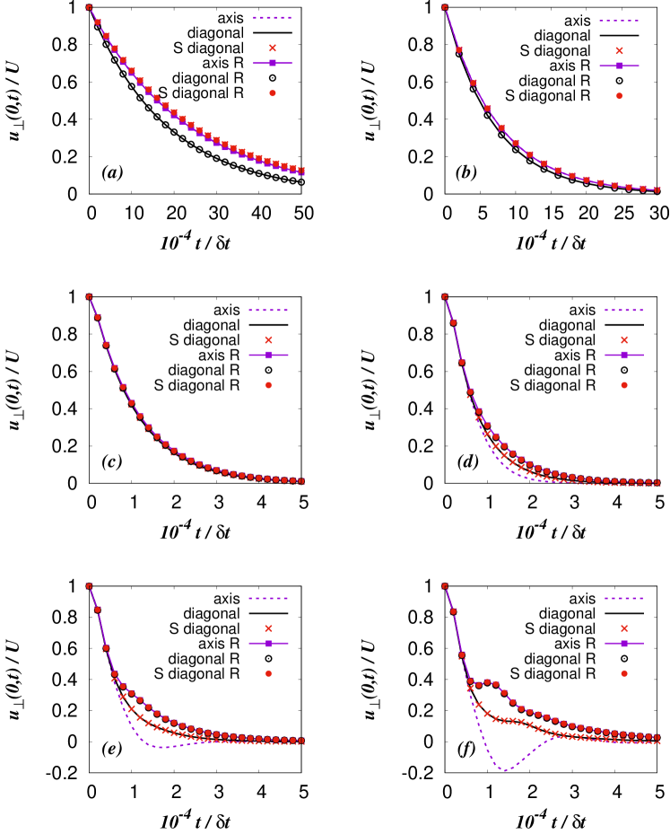
Figure 2: Evolution of the normalized peak velocity $u_{\perp}(0,t)/U$ of decaying shear waves obtained using the CTU1 numerical scheme with and without regularization, for various values of the relaxation time $\tau=$ 0.001 (a), 0.010 (b), 0.100 (c), 0.200 (d), 0.300 (e), 0.500 (f). The results which carry the symbol S in the plot keys were obtained on lattices with the spacing $\delta s=1/(128\sqrt{2})$, while the remaining results were obtained on lattices with $\delta s=1/128$. The results obtained using the regularization procedure are marked with the symbol R.

Note that $\xi_{k,\alpha}\,=\,\varsigma_{k,\alpha}|\xi_{k,\alpha}|$, where $|\xi_{k,\alpha}|$ is the modulus of $\xi_{k,\alpha}$ (the sum rule over repeated indices is not considered for the symbol $\varsigma_{k,\alpha}$). Figure 1 in Ref. dsfd2014 , as well as Figure 2 in Ref. australia2014 , illustrate the application of the CTU1 scheme (20) when $\xi_{k,x}>0$ and $\xi_{k,y}>0$. In this case, specific fractions of the neighboring distribution functions $f_{k,i-1,j}^{n}$, $f_{k,i-1,j-1}^{n}$ and $f_{k,i,j-1}^{n}$ are transported to the cell $(i,j)$ across the sides of its lower left corner and contribute to $f_{k,i,j}^{n+1}$, besides the remaining fraction of $f_{k,i,j}^{n}$.

Expanding $f_{k,i,j}^{n+1}$, $f_{k,i-\varsigma_{k,x},j}^{n}$, $f_{k,i,j-\varsigma_{k,y}}^{n}$ and $f_{k,i-\varsigma_{k,x},j-\varsigma_{k,y}}^{n}$ in Eq. (20) up to second order with respect to $\delta s$ and $\delta t$, we get

$$\partial_{t}f_{k}\,+\,\frac{1}{\,2\,}\,\delta t\,\partial_{t}^{2}f_{k}\,+\,{\bm{\xi}}_{k}\cdot\nabla f_{k} =$$

$$+\,\frac{1}{\,2\,}\,\delta s\,|\xi_{k,x}|\,\partial_{x}^{2}f_{k}\,+\,\frac{1}{\,2\,}\,\delta s\,|\xi_{k,y}|\,\partial_{y}^{2}f_{k}\,+\,\delta t\,\xi_{k,x}\xi_{k,y}\,\partial_{x}\partial_{y}f_{k}.$$ (22)

In order to get rid of the second order time derivative, we differentiate Eq. (22) with respect to time and retain only the terms up to second order in $\delta s$ and $\delta t$:

$$\partial_{t}^{2}f_{k}\,=\,\left[\,\xi_{k,x}^{2}\partial_{x}^{2}f_{k}\,+\,\xi_{k,y}^{2}\partial_{y}^{2}f_{k}\,+\,2\xi_{k,x}\xi_{k,y}\partial_{x}\partial_{y}f_{k}\,\right].$$ (23)

Thus, the final form of the evolution equations solved using the CTU1 scheme is, up to second order in $\delta s$ and $\delta t$,

$$\partial_{t}f_{k}\,+\,\xi_{k,\gamma}\,\partial_{\gamma}f_{k} = -\,\frac{1}{\,\tau\,}\,\left[\,f_{k}\,-\,f^{eq}_{k}\,\right]\,+\,F_{k}$$ (24)

$$+ \frac{1}{\,2\,}\,\delta s\,\left[\,|\xi_{k,x}|\left(1-|\xi_{k,x}|\frac{\,\delta t\,}{\delta s}\right)\partial_{x}^{2}f_{k}\,+\,|\xi_{k,y}|\left(1-|\xi_{k,y}|\frac{\,\delta t\,}{\delta s}\right)\partial_{y}^{2}f_{k}\,\right].\rule{0.0pt}{25.60747pt}$$

The last term in the square brackets of the equation above contributes to the numerical viscosity jcph2003 . One can easily see that the collision-streaming scheme, which is widely used in the two-dimensional D2Q9 LB model chen_annurev1998 ; succi_2001 ; sukop_2006 ; aidun_annurev2010 ; shan_jfm2006 , is a particular case of the CTU1 scheme (24). The D2Q9 model has nine on-lattice velocity vectors ${\bm{\xi}}_{k}$, whose Cartesian projections $\xi_{k,x}$ and $\xi_{k,y}$ take the values $0$ or $\delta s/\delta t$.

II.3.2 Second order corner transport upwind

The second order corner transport upwind (CTU2) scheme improves the accuracy of the CTU1 scheme (20) by using flux limiters. Detailed description of this very elaborated scheme can be found in Refs.leveque1996 ; leveque2002 ; trangenstein2009 . A summary is given below.

Following Ref.leveque1996 , one defines the auxiliary variables

$$R_{k,i,j}^{x,n} = f_{k,i,j}^{n}-f_{k,i-1,j}^{n},$$ (25a)

$$R_{k,i,j}^{y,n} = f_{k,i,j}^{n}-f_{k,i,j-1}^{n},\rule{0.0pt}{19.91692pt}$$ (25b)

$$S_{k,i,j}^{x,n} = \frac{1}{\,2\,}|\xi_{k,x}|\left(1-\frac{\delta t}{\,\delta s\,}|\xi_{k,x}|\right)R_{k,i,j}^{x,n}\Psi\left(\frac{\,R_{k,i-\varsigma_{k,x},j}^{x,n}\,}{R_{k,i,j}^{x,n}}\right),$$ (26a)

$$S_{k,i,j}^{y,n} = \frac{1}{\,2\,}|\xi_{k,y}|\left(1-\frac{\delta t}{\,\delta s\,}|\xi_{k,y}|\right)R_{k,i,j}^{y,n}\Psi\left(\frac{\,R_{k,i,j-\varsigma_{k,y}}^{x,n}\,}{R_{k,i,j}^{x,n}}\right),\rule{0.0pt}{28.45274pt}$$ (26b)

where $\Psi(\theta)$ is a flux limiter. In this paper we will use the monitorized centered limiter (MC) leveque1996 ; leveque2002 ; trangenstein2009 ; cejp2004

$$\Psi(\theta)={\mathrm{max}}\left\{\,0,\,{\mathrm{min}}[\,(1+\theta)/2,\,2,\,2\theta\,]\,\right\}.$$ (27)

The fluxes ${\mathcal{F}}_{i+1/2,j}$ and ${\mathcal{G}}_{i,j+1/2}$, which exit the cell $(i,j)$ in the $x$ and $y$ directions, respectively, are defined by

$${\mathcal{F}}_{k,\,i+\frac{1}{2},\,j}^{n} = f_{k,\,i+\frac{1}{2}(1-\varsigma_{k,x}),\,j}\,\xi_{k,\,x}\,+\,S_{k,\,i+1,\,j}^{x,n}$$ (28a)

$$- \frac{1}{2}\,\frac{\delta t}{\,\delta s\,}\,\xi_{k,\,x}\,\xi_{k,\,y}\,R_{k,\,i+\frac{1}{2}(1-\varsigma_{k,\,y}),\,j+\frac{1}{2}(1-\varsigma_{k,\,y})}^{y,\,n}\rule{0.0pt}{22.76219pt}$$

$$+ \frac{\delta t}{\,\delta s\,}\,\xi_{k,\,x}\,\left[\,S_{k,\,i+\frac{1}{2}(1-\varsigma_{k,\,x}),\,j}^{y,\,n}-S_{k,\,i+\frac{1}{2}(1-\varsigma_{k,\,x}),\,j+1}^{y,\,n}\,\right],\rule{0.0pt}{22.76219pt}$$

$${\mathcal{G}}_{k,\,i,\,j+\frac{1}{2}}^{n} = f_{k,\,i,\,j+\frac{1}{2}(1-\varsigma_{k,\,y})}\,\xi_{k,\,y}\,+\,S_{k,\,i,\,j+1}^{y,\,n}\rule{0.0pt}{22.76219pt}$$ (28b)

$$- \frac{1}{2}\,\frac{\delta t}{\,\delta s\,}\,\xi_{k,\,x}\,\xi_{k,\,y}\,R_{k,\,i+\frac{1}{2}(1-\varsigma_{k,\,x}),\,j+\frac{1}{2}(1-\varsigma_{k,y})}^{x,\,n}\rule{0.0pt}{22.76219pt}$$

$$+ \frac{\delta t}{\,\delta s\,}\,\xi_{k,\,y}\,\left[\,S_{k,\,i,\,j+\frac{1}{2}(1-\varsigma_{k,\,y})}^{x,\,n}-S_{k,\,i+1,\,j+\frac{1}{2}(1-\varsigma_{k,\,y})}^{x,\,n}\,\right].\rule{0.0pt}{22.76219pt}$$

The incoming numerical fluxes ${\mathcal{F}}_{i-1/2,j}\equiv{\mathcal{F}}_{(i-1)+1/2,\,j}$ and ${\mathcal{G}}_{i,\,j-1/2}\equiv{\mathcal{G}}_{i,\,(j-1)+1/2}$ are defined in a similar manner. According to the CTU2 scheme, the distribution function $f_{k,\,i,\,j}^{n}$ is updated as follows leveque1996 ; leveque2002 ; trangenstein2009 :

$$f_{k,\,i,\,j}^{n+1} = f_{k,\,i,\,j}^{n}\,-\,\frac{\delta t}{\,\delta s\,}\,[\,{\mathcal{F}}_{i+1/2,\,j}\,-\,{\mathcal{F}}_{i-1/2,\,j}\,+\,{\mathcal{G}}_{i,\,j+1/2}\,-\,{\mathcal{G}}_{i,\,j-1/2}\,]$$

$$-\,\frac{\,\delta t\,}{\,\tau\,}\,\left[\,f_{k,\,i,\,j}\,-\,f^{eq}_{k,i,j}\,\right]\,+\,\delta tF_{k}\rule{0.0pt}{22.76219pt}$$

where $f^{eq}_{k,\,i,\,j}$ and $F_{k,\,i,\,j}$ are calculated according to Eqs. (6) and (7), respectively. In this case an analytical expression for the numerical viscosity cannot be derived but it is supposed to be at the second order in the lattice spacing $\delta s$.

II.4 Numerical viscosity, anisotropy and regularization

In order to investigate possible anisotropy due to numerical effects, in this subsection we analyze the evolution of shear waves of wavelength $\lambda=2$ in an ideal gas with density $\rho=1$ at temperature $T=1$ by setting $F_{k}=0$, $1\leq k\leq K$, in the evolution equation (4). Computer simulations were performed using both the CTU1 and the CTU2 numerical schemes on a two-dimensional square lattice with $L_{x}\times L_{y}$ nodes along the Cartesian axes, where periodic boundary conditions apply. For each numerical scheme, we conducted two series of simulations with the time step $\delta t=10^{-4}$. In the first series, the wave vector ${\bm{k}}$, $|{\bm{k}}|=2\pi/\lambda$, was aligned along the horizontal axis of the square lattice and its Cartesian components were $(2\pi/\lambda,0)$. This series will be denoted as the axial (A) one. In the second series, denoted as the diagonal (D) one, the wave vector ${\mathbf{k}}$ was aligned along the diagonal direction of the square lattice after a counterclockwise rotation by an angle $\pi/4$, hence its Cartesian components were $(\pi\sqrt{2}/\lambda,\pi\sqrt{2}/\lambda)$.

To account for the numerical effects induced by the CTU1 and CTU2 schemes, two values of the lattice spacing $\delta s$ were used in each series, namely $1/128$ and $1/256$. When conducting the first series of simulations with these values of $\delta s$, the wavelength $\lambda=2$ of the shear waves was easily secured on lattices with $256\times 256$ and $512\times 512$ nodes, respectively. To match the periodic boundary conditions for $\lambda=2$ using the same values of $\delta s$ when simulating the diagonal waves, we conducted the simulations on square lattices with $362\times 362$ and $724\times 724$ nodes, respectively, as suggested in zhang2006pre .

Let ${\bm{u}}({\bm{x}},t)$ be the fluid velocity vector in the node ${\bm{x}}=(i\delta s,j\delta s)$ of the lattice at time $t$. The components of the vector ${\bm{u}}({\bm{x}},t)$, which are parallel or perpendicular to the wave vector $\bm{k}$, are denoted $u_{\parallel}({\bm{x}},t)$ and $u_{\perp}({\bm{x}},t)$, respectively. In both the series of simulations, the shear waves were initialized according to:

$$u_{\parallel}({\bm{x}},0) = 0$$ (30a)

$$u_{\perp}({\bm{x}},0) = U\cos({\bm{k}}\cdot{\bm{x}})$$ (30b)

with $U=0.01$. When the fluid is not too far from the equilibrium (i.e., when the relaxation time is small enough), the fluid evolves according to the Navier-Stokes equations. For shear waves, we have $u_{\parallel}({\mathbf{x}},t)=0$ and there is no spatial variation of the velocity vector along the direction perpendicular to the wave vector. Under these circumstances, and assuming that the fluid is isothermal and incompressible, the shear wave equation reads

$$\partial_{t}u_{\perp}({\bm{x}},t)\,-\,\nu_{app}\,\partial_{\parallel}^{2}u_{\perp}({\bm{x}},t)=0$$ (31)

where $\nu_{app}$ is the apparent value of the kinematic viscosity jcph2003 and $\partial_{\parallel}^{2}$ denotes the second order space derivative along the direction of the wave vector. As described in jcph2003 , the value of the apparent viscosity can be determined at time $t$ according to

$$\nu_{app}\,=\ \frac{1}{\,k^{2}t\,}\,\log\,\frac{\,u_{\perp}(0,0)\,}{\,u_{\perp}(0,t)\,}$$ (32)

where $k=|{\bm{k}}|$.

Figure 1 shows the evolution of the normalized peak velocity $u_{\perp}(0,t)/U$ for six values of the relaxation time $\tau$. When using the CTU1 scheme and small values of the relaxation time ($\tau=0.001,0.01$), the evolution of the shear waves in the two directions (axial and diagonal) differs significantly for both values of the lattice spacing $\delta s$ considered in our simulations. This is due to the anisotropy of the numerical effects, which plague the solutions of hyperbolic partial differential equations in multi-dimensional spaces sescu2014 ; sescu2015 . The numerically induced anisotropy reduces significantly when using higher order schemes, as seen in Fig. 1, where the evolution of the shear waves orientated along both the axial and the diagonal direction is quite identical when using the CTU2 scheme with $\tau=0.001,0.01$. Although both the CTU1 and the CTU2 simulations give close results for $\tau=0.1$, regardless of the orientation of the shear waves or of the value of the lattice spacing $\delta s$, Fig. 1 shows that the evolution of the axial and the diagonal shear waves differ again when $\tau$ is further increased. More precisely, when $\tau>0.1$, the evolution of the shear waves becomes more and more anisotropic and, apparently, it no longer depends either on the order of the CTU scheme used to conduct the simulation or on the lattice spacing $\delta s$. This kind of anisotropy, which manifests for higher values of $\tau$, regardless of the numerical scheme used to evolve the distribution functions $f_{k}$, can be reduced by using a regularization procedure, as will be discussed further in this subsection.

In order to understand all the features mentioned above, we refer to Ref. jcph2003 , where it is assumed that the apparent value $\nu_{app}$ of the kinematic viscosity of a fluid, observed during simulations conducted with finite-difference LB models, is always the sum of two terms, the physical (theoretical) value of the viscosity $\nu_{phys}$ and the numerical viscosity $\nu_{num}$

$$\nu_{app}\,=\,\nu_{phys}\,+\,\nu_{num}.$$ (33)

When the fluid satisfies the Navier-Stokes equations, it can be shown that the application of the Chapman - Enskog method jcph2003 gives

$$\nu_{phys}=\rho\tau T$$ (34)

which is a constant quantity in the case of our shear wave simulations. Table 2 shows the values of the apparent viscosity $\nu_{app}^{axial}$ and $\nu_{app}^{diagonal}$, as determined at $t=20$ using Eq. (32) when using the CTU1 and the CTU2 schemes to simulate the shear wave decay with $\tau\in\{0.001,0.01\,\}$. For convenience, in Table 3 we show also the corresponding values of the numerical viscosity, derived from Table 2 according to Eqs. (33) and (34), in the case of the CTU1 scheme.

Inspection of the results in Table 3 reveals that the numerical viscosity of the CTU1 scheme is practically independent of the relaxation time $\tau$ and depends only on the orientation of the shear waves, as well as on the lattice spacing $\delta s$. For each orientation (axial or diagonal) of the shear waves, it is easy to observe that

$$\nu_{num}^{orientation}({\mathrm{CTU1}},\tau,\delta s=1/128)\,/\,\nu_{num}^{orientation}({\mathrm{CTU1}},\tau,\delta s=1/256)\simeq 2$$ (35)

This agrees with Eq. (24), where the spurious (last) term depends linearly on $\delta s$. Moreover, for both values of $\delta s$ in Table 3, one can see that

$$\nu_{num}^{diagonal}({\mathrm{CTU1}},\tau,\delta s)\,/\,\nu_{num}^{axial}({\mathrm{CTU1}},\tau,\delta s)\simeq\sqrt{2}$$ (36)

which is not a surprise since the distance between the lattice nodes along the diagonal direction of the lattice is $\delta s\sqrt{2}$. As the value of $\tau$ increases, the relative contribution of the numerical viscosity $\nu_{num}$ to the apparent viscosity, Eq. (33), becomes smaller. This explains why the evolution of the axial and the diagonal shear waves becomes quite identical, as seen in Fig. 1 when using the CTU1 scheme with $\tau=0.1$.

The numerical effects introduced by the CTU2 scheme are much smaller than in the case of the CTU1 scheme. For this reason, the evolution of shear waves, as seen for $\tau\leq 0.1$ in the CTU2 simulations reported in Fig. 1, is quite independent on their orientation, as well as on the value of $\delta s$. Moreover, in Table 2 one can see that the CTU2 values of the apparent viscosity, reported for $\tau=0.001$ and $\tau=0.01$, are close enough to the corresponding physical values given by Eq. (34).

Table 2: Apparent values of the viscosity of the shear waves orientated along the axial or the diagonal direction of a square lattice, calculated at $t=20$ using the first and the second order corner transport schemes, for small values of the relaxation time $\tau$ and two values of the lattice spacing $\delta s$.

				$\nu_{app}^{axial}$				$\nu_{app}^{diagonal}$
$\tau$		$\delta s$		CTU1		CTU2		CTU1		CTU2
0.001		1/128		4.3685e-03		9.5054e-04		5.5900e-03		9.5024e-04
		1/256		2.6343e-03		9.5002e-04		3.2201e-03		9.4990e-04
0.010		1/128		1.3344e-02		9.9367e-03		1.4572e-02		9.9380e-03
		1/256		1.1615e-02		9.9356e-03		1.2205e-02		9.9373e-03

Table 3: Numerical viscosities observed during the simulation of shear waves with the CTU1 scheme at small values of the relaxation time $\tau$, as calculated from Table 2 by subtracting the corresponding values of $\nu_{phys}=\rho\tau T$.

$\tau$		$\delta s$		$\nu_{num}^{axial}({\mathrm{CTU1}},\tau,\delta s)$				$\nu_{num}^{diagonal}({\mathrm{CTU1}},\tau,\delta s)$
0.001		1/128		3.3685e-03				4.5900e-03
		1/256		1.6343e-03				2.2201e-03
0.010		1/128		0.3344e-02				0.4572e-02
		1/256		0.1615e-02				0.2205e-02

For $\tau>0.1$, the plots in Fig. 1 show that the evolution of the shear waves becomes more and more anisotropic and does not depend either on the numerical scheme or on the lattice spacing $\delta s$. This kind of anisotropy, which develops when the fluid system lies further and further from the equilibrium state (i.e., when the relaxation time $\tau$ becomes large enough) is present also in the collision-streaming LB models zhang2006pre ; latt2006mcs ; colosqui2009pof ; colosqui2010pre ; montessori2014pre ; mattila_pof2017 and originates from the non-equilibrium part of the distribution function, which overpasses the space of the tensor Hermite polynomials up to order $N$, used in the model.

Let us assume that at time $t=0$, the functions $f_{k}$, which evolve according to Eq. (4), are expressed as an expansion up to the order $N=3$

$$f_{k}\equiv f_{k}({\bm{x}},t)\,=\,w_{k}\,\sum_{\ell=0}^{N}\,\frac{1}{\ell!}\,{\bm{a}}^{(\ell)}_{\alpha_{1}\ldots\alpha_{\ell}}({\bm{x}},t)\,{\bm{\mathcal{H}}}^{(\ell)}_{\alpha_{1}\ldots\alpha_{\ell}}({\bm{\xi}}_{k}),$$ (37)

with respect to the tensor Hermite polynomials ${\bm{\mathcal{H}}}^{(\ell)}_{\alpha_{1}\ldots\alpha_{\ell}}({\bm{\xi}}_{k})$, in a similar way as the expansion (5) of $f^{eq}$. Since the functions $f_{k}$ are subjected to the transport operator ${\bm{\xi}}_{k}\cdot{\bm{\nabla}}$ in the evolution equation (4), the application of the recurrence relation shan_jfm2006

$$\xi_{\alpha}{\bm{\mathcal{H}}}^{(\ell)}_{\alpha_{1}\ldots\alpha_{\ell}}({\bm{\xi}})\,=\,{\bm{\mathcal{H}}}^{(\ell+1)}_{\alpha\alpha_{1}\ldots\alpha_{\ell}}({\bm{\xi}})\,+\,\sum_{k=1}^{\ell}\,\delta_{\alpha\alpha_{k}}\,{\bm{\mathcal{H}}}^{(\ell-1)}_{\alpha_{1}\ldots\alpha_{k-1}\alpha_{k+1}\ldots\alpha_{\ell}}({\bm{\xi}})$$ (38)

reveals that after the first time step the series expansion (37) of $f_{k}$ acquires a supplementary term of order $N+1$. Subsequent time steps performed during the computer simulation further increase the order of the tensor Hermite polynomials in the expansion of $f_{k}$ and, thus, $f_{k}$ will lie outside the space where $f_{k}^{eq}$ are defined, that is, the space generated by the tensor Hermite polynomials up to a certain order $N$ (e.g., $N=3$ as in this paper or $N=2$ as in the D2Q9 LB model widely used in the literature). This behavior originates from the recurrence property (38) of Hermite polynomials and is specific to any LB models based on the Gauss-Hermite quadrature, including the one used in this paper. However, when Cartesian projections of all the velocity vectors ${\bm{\xi}}_{k}$, $k=1,\,2,\,\ldots\,K$, used in the LB model are roots of the Hermite polynomial $H^{Q}(\xi)$ of order $Q=N+1$, the tensor Hermite polynomials of order $N+1$ in Eq. (38) vanish when all indices $\alpha,\,\alpha_{1},\,\ldots\alpha_{\ell=N}$ are equal. This feature of the LB model used in this paper, which does not allow the order of the series expansion of $f_{k}$ to increase indefinitely during the advection process ijmpf , is further discussed in the Appendix.

It is known that the terms in the expansion (37) of the distribution functions $f_{k}$, which contain Hermite tensors of order higher than the order $N$ used in the expansion of the equilibrium distribution functions $f_{k}^{eq}$, are at the origin of numerous issues (numerical instabilities, anisotropy, low accuracy, etc.) which manifest at higher values of the relaxation time $\tau$ niu2007pre ; suga2010pre ; suga2013fdr ; zhang2006pre ; latt2006mcs ; colosqui2009pof ; colosqui2010pre ; montessori2014pre ; mattila_pof2017 . To reduce these problems, one can use a regularization procedure niu2007pre ; suga2010pre ; suga2013fdr ; zhang2006pre ; latt2006mcs ; colosqui2009pof ; colosqui2010pre ; montessori2014pre ; mattila_pof2017 . Following this recipe, the non-equilibrium part $f^{neq}=f_{k}-f_{k}^{eq}$ of the functions $f_{k}$, which enters the BGK collision term in the evolution equation (4), is replaced at each time step by zhang2006pre

$$\hat{f}_{k}^{neq}\,=\,w_{k}\,\left[\,\frac{1}{\,2!\,}\,{\bm{\mathcal{H}}}^{(2)}_{\alpha\beta}({\bm{\xi}}_{k})\sum_{k^{\prime}=1}^{K}f_{k^{\prime}}^{neq}{\bm{\xi}}_{k^{\prime},\alpha}{\bm{\xi}}_{k^{\prime},\beta}\,+\,\frac{1}{\,3!\,}\,{\bm{\mathcal{H}}}^{(3)}_{\alpha\beta\gamma}({\bm{\xi}}_{k})\sum_{k^{\prime}=1}^{K}f_{k^{\prime}}^{neq}{\bm{\xi}}_{k^{\prime},\alpha}{\bm{\xi}}_{k^{\prime},\beta}{\bm{\xi}}_{k^{\prime},\gamma}\,\right]$$ (39)

Application of the regularization procedure at every time step eliminates the terms of order higher than $N=3$ in the Hermite expansion of the distribution functions $f_{k}$, $k=1,\,2,\,\ldots K$, hence both $f_{k}$ and $f_{k}^{eq}$ remain in the space generated by the tensor Hermite polynomials of order at most $N=3$.

In Fig. 2, we compare the evolution of the normalized peak velocity $u_{\perp}(0,t)/U$ of shear waves of wavelength $\lambda=2$. For each value of the relaxation time $\tau$, the plots in this figure show the decay of the normalized peak velocity in three cases. In the first case, the wave vector $\mathbf{k}$ of the shear waves is oriented along the horizontal axis of a square lattice lattice with spacing $\delta s=1/128$. In the second and third cases, the wave vector $\mathbf{k}$ is oriented along the diagonal of the square lattices with spacings $\delta s=1/128$ and $\delta s=1/(128\sqrt{2})$, respectively. The results obtained on the lattice with the smaller spacing ($\delta s=1/(128\sqrt{2})$) carry the symbol S in the corresponding plot keys. In all cases, the simulations were conducted using the CTU1 scheme with or without application of the regularization procedure, Eq. (39) above. The results obtained using the regularization procedure carry the symbol R in the plot keys.

Inspection of the plots in Fig. 2 reveals that the application of the regularization procedure does not change the evolution of shear waves for $\tau\leq 0.1$, i.e., when the fluid is not far from the equilibrium. Moreover, for $\tau<0.1$ and $\delta s=1/128$ one can see that the axial and the diagonal shear waves evolve differently because of the anisotropy of the spurious viscosity, as discussed previously. Furthermore, for these small values of $\tau$, the evolution of the diagonal waves on the square lattice with $\delta s=1/(128\sqrt{2})$ (the results marked with S in the plot keys) agrees to the evolution of the axial waves on the lattice with $\delta s=1/128$, as expected since the numerical viscosities are quite identical in these cases. For $\tau=0.1$, the evolution of the shear waves is quite identical, regardless of their orientation or the value of $\delta s$. As discussed previously, this happens because the relative contribution of the numerical viscosity to the apparent value of the viscosity becomes negligible when $\tau$ is large enough. When no regularization procedure is applied, the simulation results for $\tau>0.1$ become anisotropic again. Furthermore, one can see that the evolution of the diagonal shear waves is identical, despite of the different values of the lattice spacing $\delta s$. The application of the regularization procedure during the simulations fully restores the isotropy, as already known in the literature zhang2006pre ; latt2006mcs ; colosqui2009pof ; colosqui2010pre ; montessori2014pre ; mattila_pof2017 .

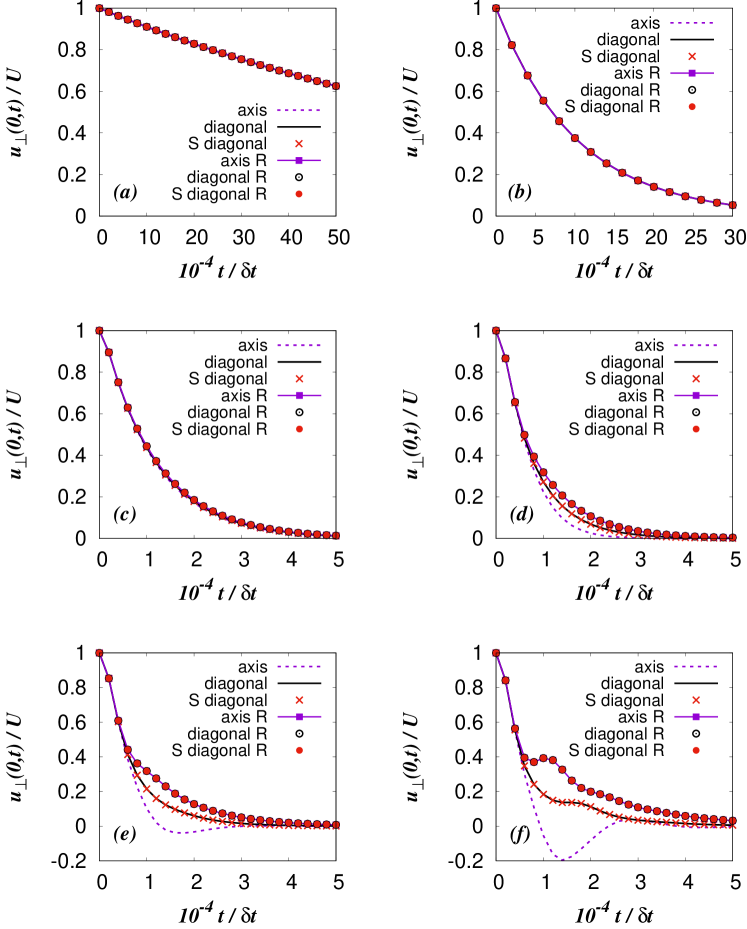
Figure 3: Evolution of the normalized peak velocity $u_{\perp}(0,t)/U$ of decaying shear waves obtained using the CTU2 numerical scheme with and without regularization, for various values of the relaxation time $\tau=$ 0.001 (a), 0.010 (b), 0.100 (c), 0.200 (d), 0.300 (e), 0.500 (f). The results which carry the symbol S in the plot keys were obtained on lattices with the spacing $\delta s=1/(256\sqrt{2})$, while the remaining results were obtained on lattices with $\delta s=1/256$. The results obtained using the regularization procedure are marked with the symbol R.

We checked the regularization also for the CTU2 scheme. The results shown in Fig. 3) confirm again that the application of the regularization procedure cures the anisotropy which appears at large values of the relaxation time ($\tau>0.1$).

Since the LB model introduced in this paper is used to investigate the behavior of a cavitation bubble, which obeys the Navier-Stokes equations for an isothermal fluid governed by the van der Waals equation of state, Eq. (14), the values of the relaxation time $\tau$ to be considered further during the simulations need to be small enough ($\tau\leq 0.01$) in order to ensure the correct recovery of these equations ambrus_pre2012 ; piaud_ijmpc2014 ; sspre2005 ; pre2014 ; sone ; karniadakis . For this reason, we did not use the regularization procedure during the simulations reported in Section III since it is not necessary, as just seen.

II.5 Liquid - vapor phase diagram

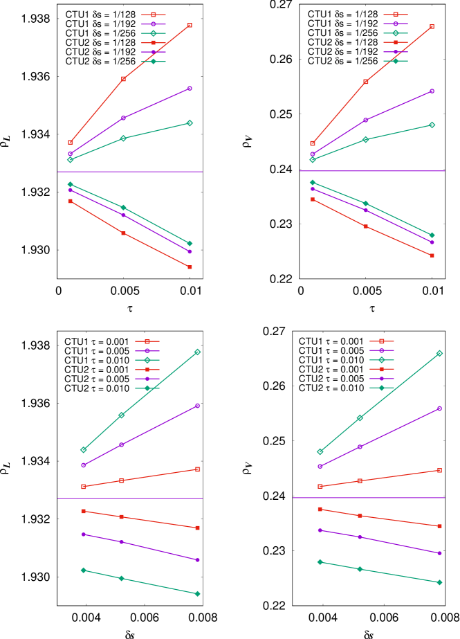
Figure 5: Dependence of the numerical liquid and vapor densities $\rho_{L}$ and $\rho_{V}$, respectively, on the relaxation time $\tau$ and on the lattice spacing $\delta s$ at temperature $T=0.80$, obtained with the CTU1 and the CTU2 numerical schemes ($\delta t=10^{-4}$). The horizontal line in each plot shows the corresponding theoretical density value computed using the Maxwell construction.

The liquid-vapor phase diagram of the present model is shown in Fig. 4 was determined by inspecting the profile of the planar liquid-vapor interface in the stationary case at various temperatures. The simulations were conducted using the CTU2 numerical scheme with the relaxation time $\tau=0.001$, the time step $\delta t=10^{-4}$, and the lattice spacing $\delta s=1/256$. Good agreement between the LB values of the liquid and vapor densities and the corresponding values derived by the Maxwell construction is seen for all temperatures $T\geq 0.70$. For lower temperatures, the values of the vapor density become significantly smaller than the values derived by the Maxwell construction (e.g., at T=0.60 , their relative difference approaches $8\%$). As seen in Fig. 5, when the relaxation time $\tau$ or the lattice spacing $\delta s$ decrease, the values of both the liquid and the vapor densities approach the corresponding values derived using the Maxwell construction, regardless of the numerical scheme (CTU1 or CTU2). This is not a surprise if we recall that the LB simulation results approach the results of the Navier-Stokes equations when the relaxation time $\tau$ decreases shan_jfm2006 ; ambrus_pre2012 ; ambrus_jcph2016 ; piaud_ijmpc2014 ; sspre2005 ; pre2014 ; sone ; karniadakis and, moreover, the numerical errors induced by the finite volume schemes always reduce when the lattice spacing decreases.

III Simulation results

III.1 Critical radius for bubble growth in a quiescent liquid

In this subsection, we will consider the kinetics of a vapor bubble expanding in a superheated liquid. Let us denote by $\rho_{L}$ and $\rho_{V}$ the values of the liquid and vapor densities of the van der Waals fluid, as calculated from the non-dimensionalized equation of state (14) according to the Maxwell construction. When a vapor bubble of density $\rho_{V}$ and initial radius $R(t=0)$ is placed in a superheated liquid at density $\rho_{ext}<\rho_{L}$, it will shrink or grow depending on its initial size since the system will tend to locally decrease its Gibbs free energy density, the latter being given by the Helmholtz free energy density $\psi$ plus the pressure. Indeed, the system can reduce the Helmholtz free energy by increasing the bubble size via phase separation of some of the metastable liquid to the coexistence densities. On the other hand this determines an increase of the interfacial free energy as the bubble grows. The balance between these two contributions, under the constraint of local mass conservation, causes either the growth or the collapse of the bubble. It has been shown laurila-2012 that the critical radius $R_{c}$ of the bubble that will neither shrink or grow is

$$R_{c}^{pred}=-\frac{\sigma}{2}\Big{\{}\Big{[}\psi(\rho_{V},T)-\psi(\rho_{ext},T)\Big{]}+\frac{\rho_{ext}-\rho_{V}}{\rho_{L}-\rho_{ext}}\Big{[}\psi(\rho_{L},T)-\psi(\rho_{ext},T)\Big{]}\Big{\}}^{-1}$$ (40)

where $\sigma$ is the surface tension between liquid and vapor at coexistence and $\psi(\rho,T)$ is given by Eq. (12). The surface tension was numerically computed by using its definition

$$\sigma=\frac{\kappa}{2}\int dx\big{[}\nabla\rho(x)\big{]}^{2}$$ (41)

where the numerical values of the density $\rho$ across a plane interface with liquid and vapor phases relaxed to equilibrium, were used.

In order to test the prediction (40) in our model, vapor bubbles at density $\rho_{V}=0.2396$ with different values of the initial radius $R(t=0)$ were centered in the lattice domain and surrounded by a superheated liquid at density $\rho_{ext}<\rho_{L}=1.9327$. The fluid density was allowed to evolve freely within a circle of constant radius $R_{BC}=[L/2-1/(2\delta s)]\delta s$, where $L=L_{x}=L_{y}$ is the number of nodes on each Cartesian axis. Outside this circle, the liquid density was set to the prescribed value $\rho_{ext}$ according to the following procedure. At time $t=n\delta t$, periodic boundary conditions were used to evolve the distribution functions in all nodes of the lattice. Before processing the next time step, the local fluid density $\rho_{i,j}^{n}$ was evaluated in each lattice node $(i,j)$, $0\leq i,j<L$ and, if the node $(i,j)$ is located outside the circle of radius $R_{BC}$, the values of the corresponding distribution functions $f_{k;i,j}^{n}$ were rescaled by the factor $\rho_{ext}/\rho_{i,j}^{n}$.

In order to explore the effect of the lattice spacing on the accuracy of the computer results, we conducted two series of computer simulations with the CTU2 numerical scheme. In the first series, we used a lattice with $L=2048$ nodes on each axis and spacing $\delta s=1/128$, while in the second series we used three lattices with $L=4096,\,2048$ and $1024$ nodes, all with spacing $\delta s=1/256$. The other parameters of these runs were $\delta t=10^{-4}$, $\tau=10^{-3}$, $T=0.8$ and $\kappa=10^{-4}$. The values of the surface tension $\sigma$ are quite independent on the lattice spacing ($\sigma=4.8754\times 10^{-3}$ and $\sigma=4.8747\times 10^{-3}$ for $\delta s=1/128$ and $\delta s=1/256$, respectively).

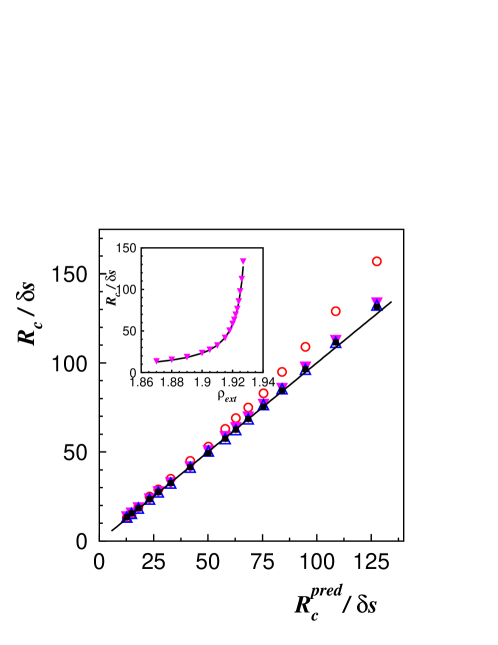
Figure 6: Values of the critical bubble radius $R_{c}$ from LB simulations versus the theoretical predictions of Eq. (40) represented by the full line. The marks correspond to various values of the external density $\rho_{ext}$. The LB results were obtained with the CTU1 scheme on a lattice with spacing $\delta s=1/128$ and size $L=2048$ ($\circ$) and with the CTU2 scheme on lattices with $\delta s=1/256$ and sizes $L=4096(\blacktriangledown),\,2048(\triangle),\,1024(\blacksquare)$. Inset: Values of $R_{c}$ from LB simulations with the CTU2 scheme on the lattice with $\delta s=1/256$ and size $L=4096(\blacktriangledown)$, and from the theoretical predictions $(-\!\!\!-\!\!\!-)$ as a function of the external density $\rho_{ext}$.

The evolution of the bubbles was monitored for several values of $\rho_{ext}$ in the range $[1.870--1.927]$. For each value of $\rho_{ext}$, the critical value $R_{c}$ of the bubble was estimated as $R_{c}=(R_{g}+R_{s})/2$ where $R_{g}$ is the initial smallest radius of a growing bubble and $R_{s}$ is the initial largest radius of a shrinking bubble with $R_{g}=R_{s}+\delta s$. The numerical values of $R_{c}$ are plotted in Fig. 6, where they are compared to the ones predicted by Eq. (40). We note that Eq. (40) predicts $R_{c}^{pred}$ to increase with $\rho_{ext}$ (see the inset of Fig. 6). It appears that numerical results of $R_{c}$ agree quite well with $R_{c}^{pred}$ for the smaller value of $\delta s$ with a slight overestimation at larger values of $\rho_{ext}$. For this reason the rest of the study performed in this paper will be done using the value $\delta s=1/256$ of the lattice spacing. Finally, no dependence of the critical radius on the system size $L$ can be appreciated, as it appears from Eq. (40). This is quite well confirmed in Fig. 6, when comparing the corresponding values of $R_{c}$ obtained on the three lattices with $\delta s=1/256$.

III.2 Bubble growth in a quiescent liquid: The Rayleigh-Plesset equation

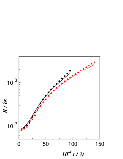
Figure 7: The radius $R$ of the growing bubble in a quiescent liquid as a function of time for lattice size $L=4096(\bullet),6144(\blacktriangle)$ from the lattice Boltzmann simulations. The full and dashed lines correspond to the numerical solutions of the RP equation (48) for $L=4096,6144$, respectively.

As we saw above, a vapor bubble immersed in a superheated liquid at density $\rho_{ext}<\rho_{L}$ will grow when its initial radius is larger than the corresponding critical value $R_{c}$. For some values of $\rho_{ext}$, we followed the evolution of the radius $R(t)$ of vapor bubbles of initial size $R>R_{c}$ and density $\rho_{V}=0.2396$ on lattices of size $L=4096,6144$, with $\delta s=1/256$ and density fixed at the value $\rho_{ext}$ at the nodes outside the circle of radius $R_{BC}$, as already described in the previous section. The evolution of the bubble radius was followed after the relaxation of the initial sharp interface. The bubble keeps a circular shape during the overall process. The results of $R(t)$ versus time shown in Fig. 7 were obtained for an initial bubble radius $R=77\,\delta s$, which is larger than the value $R_{c}=76.5\,\delta s$ corresponding to the choice $\rho_{ext}=1.923$. Results for other values of $\rho_{ext}$ are similar. Before commenting the results, we discuss the equation which describes the evolution of the bubble radius for the present problem.

The time behavior of the radius of a spherical vapor bubble in an infinitely large liquid domain at constant temperature is described by the Rayleigh - Plesset (RP) equation brennen-1995 . In the following we will derive for completeness its form in the two-dimensional case. We consider a circular vapor bubble of radius $R$ in a liquid whose density $\rho_{L}$ and dynamic viscosity $\mu_{L}$ are assumed constant. The radial position will be denoted by the distance $r$ from the bubble center ($r=0$) located in the middle of the system, the pressure by $p(r,t)$, and the radial outward velocity by $u(r,t)$. The tangential component of the velocity is null since the system has central symmetry. The liquid far field boundary is located at $r_{\infty}=R_{BC}$, where the pressure is $p_{\infty}$. The pressure $p_{B}$ and the density $\rho_{V,B}$ inside the bubble are assumed to be uniform. In order to guarantee mass conservation it is taken

$$u(r,t)=\frac{F(t)}{r}$$ (42)

where $F(t)$ is a function to be determined in order to satisfy the continuity equation which for an incompressible fluid reads as

$$\frac{1}{r}\frac{\partial}{\partial r}\big{[}ru(r,t)\big{]}=0.$$ (43)

$F(t)$ and $R(t)$ are related by a kinematic boundary condition at the bubble interface. Assuming that there is no mass flow across this interface, it has to be $u(R,t)=dR/dt$ and hence

$$F(t)=R\frac{dR}{dt}.$$ (44)

Equation (44) holds also in the presence of evaporation or condensation at the interface under the hypothesis that $\rho_{L}>>\rho_{V,B}$ brennen-1995 .

In the case of a Newtonian liquid, the Navier-Stokes equation for the radial velocity is

$$\frac{\partial u(r,t)}{\partial t}+u(r,t)\frac{\partial u(r,t)}{\partial r}=-\frac{1}{\rho_{L}}\frac{\partial p(r,t)}{\partial r}+\frac{\mu_{L}}{\rho_{L}}\Big{[}\frac{1}{r}\frac{\partial}{\partial r}\big{(}r\frac{\partial u(r,t)}{\partial r}\big{)}-\frac{u(r,t)}{r^{2}}\Big{]}.$$ (45)

Substituting Eq. (42) into Eq. (45) and then integrating from $R$ to $r_{\infty}$ yields

$$\ln\Big{(}\frac{r_{\infty}}{R}\Big{)}\frac{dF(t)}{dt}-\frac{F^{2}(t)}{2}\Big{(}\frac{1}{R^{2}}-\frac{1}{r_{\infty}^{2}}\Big{)}=\frac{p(R)-p_{\infty}}{\rho_{L}}.$$ (46)

Moreover, a pressure boundary condition on the interface can be introduced which is obtained by fixing to zero the total force per unit length on the interface in the absence of mass transport across the boundary brennen-1995 :

$$p(R)=p_{B}-\frac{\sigma}{R}-\frac{2\mu_{L}}{R}\frac{dR}{dt}.$$ (47)

Substituting Eqs. (44) and (47) into Eq. (46) delivers the final form of the two-dimensional RP equation

$$\ln\left(\frac{r_{\infty}}{R}\right)\left[\left(\frac{dR}{dt}\right)^{2}+R\frac{d^{2}R}{dt^{2}}\right]-\frac{1}{2}\left[1-\frac{R^{2}}{r_{\infty}^{2}}\right]\left(\frac{dR}{dt}\right)^{2}+\frac{\sigma}{\rho_{L}R}+\frac{2\mu_{L}}{\rho_{L}R}\frac{dR}{dt}=\frac{p_{B}(t)-p_{\infty}(t)}{\rho_{L}}.$$ (48)

Some comments are here in order about Eq. (48). It is evident that the growth of the bubble radius $R$ depends on the spatial extension $r_{\infty}$ of the system differently from the three-dimensional case. This is due to the $1/r$ dependence of $u(r,t)$ in Eq. (42) which gives rise to the logarithmic term in RP equation. Once $p_{\infty}(t)$ is given, RP equation can be solved to find $R(t)$ if $p_{B}(t)$ is known. We solved it numerically by using a Runge-Kutta method to compare the results to the output of LB simulations. To this purpose the values of $\rho_{L}$, $\mu_{L}$, and $\sigma$ are the ones of the present LB model. Moreover, $p_{B}(t)$ and $p_{\infty}(t)$ were measured plugging into the EOS the values of density at the bubble center ($r=0$) and at the domain boundary ($r=r_{\infty}$), respectively, obtained from the LB simulations. The initial values of $R$ and $dR/dt$ were taken from the LB runs after the initial relaxation of the bubble interface.

The evolution of the bubble radius $R(t)$ is plotted in Fig. 7 for both the numerical solutions of RP equation and the LB simulations on lattices with $L\times L$ nodes. Since $r_{\infty}/\delta s=L/2-1/(2\delta s)$ is a finite quantity in our model, the results of the LB simulations are expected to depend on the lattice size $L$. Indeed, although both the LB results reported in Fig. 7 are quite in good agreement to the numerical solutions of the RP equation only in the early stage of the bubble growth process, the results on the smaller lattice start to deviate from the predictions of the RP equation at time $t_{4096}\simeq 7\times 10^{5}\delta t$, while the results on the larger lattice are still consistent up to $t_{6144}\simeq 10^{6}\delta t$. This is due to the fact that the RP equation relies on the implicit assumption of an infinite liquid domain where the ratio $r_{\infty}/R(t)$ is very large. When this ratio is small, the first two terms in the RP equation (48) become negligible and the RP equation loses its meaning. In the case of the larger lattice, this ratio is $r_{\infty}/R(t_{6144})\simeq 2$ and continues to reduce at times $t>t_{6144}$, worsening the agreement between the LB simulation results and the RP equation. The present model is thus capable to account for the bubble growth up to a lattice-size dependent time $t_{L}$, while remaining in good agreement to the RP equation until $R(t_{L})/R(0)\simeq 20$. This value is considerably larger than the one ($\simeq 5$) reached in previous studies chen-2010 ; chen-2011 .

III.3 Bubble growth under shear flow

The behavior of an equilibrated vapor bubble of density $\rho_{V}$ and dynamic viscosity $\mu_{V}$ with radius $R$ in a liquid with density $\rho_{L}$ and dynamic viscosity $\mu_{L}$ under shear flow received considerable attention in the past acrivos-stone ; rallison-1984 ; brennen-1995 . Here we will briefly sketch the phenomenology. For weak flows such that the capillary number $\displaystyle Ca=\frac{\mu_{L}\dot{\gamma}R}{\sigma}<<1$, $\dot{\gamma}$ being the shear rate, the bubble is deformed assuming in the stationary regime an elliptical shape whose principal axis forms a tilt angle $\theta\simeq\pi/4$ with the flow direction. When increasing the shear rate, the equilibrium shape of the bubble is more elongated with $\theta$ decreasing to zero independently on the value of the viscosity ratio $\lambda=\mu_{V}/\mu_{L}$. A further increase of the shear rate would deform the bubble into a point-ended shape until its break-up at small values of $\lambda$, while for $\lambda>\lambda_{c}\simeq 4$ the bubble would attain an equilibrium elliptical shape with $\theta\simeq 0$.

In the present study a lattice of size $L\times L$ with $L=6144$ was confined by two permeable horizontal walls shearing with velocities ${\mathbf{u}}_{top}=(u_{w},0)$ and ${\mathbf{u}}_{bot}=(-u_{w},0)$ along the $x$ axis, respectively. In the lattice nodes outside the walls, i.e., in the ghost nodes $(i,j)$, $0\leq i<L$, $j\in\{-2,\,-1,\,L,\,L+1\}$, the distribution functions $f_{k;i,j}^{t}$ were set according to Eq. (6), where $\rho$ was replaced by $\rho_{ext}$ and

$${\mathbf{u}}=\left\{\begin{array}[]{rcl}{\mathbf{u}}_{top}&,&j\in\{L,\,L+1\}\\ {\mathbf{u}}_{bot}&,&j\in\{-2,\,-1\}\end{array}\right.$$ (49)

Periodic boundary conditions were applied in the horizontal direction.

A bubble of initial radius $R=26\delta s$ and density $\rho_{V}=0.23967$ was placed in a superheated liquid with density $\rho_{ext}=1.90$ at $T=0.80$. Under these conditions, the bubble grows in a quiescent liquid as previously seen. Various values of the wall velocity $u_{w}$ were considered in order to vary the shear rate $\dot{\gamma}=2u_{w}/(L\delta s)$. The highest value of $u_{w}$ was such to have Mach number $Ma=u_{w}/c_{s}\simeq 0.5$, where $c_{s}=\sqrt{dp^{w}/d\rho}\simeq 1.7$ is the sound velocity in the liquid phase. We remark that the present model, being accurate at the third order with the correct quadrature, is not limited to the incompressible regime chen-2008 . Because of the large system size here adopted to follow the growth of the bubble on long time scales, the values of $\dot{\gamma}$ are small so we considered the relaxation time $\tau=10^{-2}$ in order to increase the liquid viscosity $\mu_{L}$ ($=\rho_{L}T\tau$) and, thus, accessing larger values of the capillary number. The fluid velocity was initialized to be the one corresponding to a linear flow profile with shear rate $\dot{\gamma}$. The bubble grew by the same mechanism previously described being, in the meanwhile, deformed and rotated by shear.

The morphology and alignment with the flow were studied by using the gyration tensor of the bubble, defined as

$$T_{\alpha\beta}=\frac{1}{N_{b}}\sum_{i\in bubble}(r_{i,\alpha}-{\bar{r}_{\alpha}})(r_{i,\beta}-{\bar{r}_{\beta}})$$ (50)

where the sum is over the $N_{b}$ lattice sites belonging to the bubble, whose position vectors are ${\bm{r}}_{i}$. The position vector of the center of the bubble is ${\bm{\bar{r}}}=\sum_{i\in bubble}{\bm{r}}_{i}/N_{b}$. The two eigenvalues $\Lambda_{M}$ and $\Lambda_{m}$ with $\Lambda_{M}>\Lambda_{m}$ of the gyration tensor were then used to characterize the bubble shape. Indeed, in the case of an ellipse with semi-axes $a$ and $b$ with $a>b$ it can be shown that $a=2\sqrt{\Lambda_{M}}$ and $b=2\sqrt{\Lambda_{m}}$. This will be the way here adopted to estimate the typical size of the elliptical bubble. However, we checked that the results later presented do not depend on this particular way of estimating $a$ and $b$. Indeed, for a comparison $a$ and $b$ were also computed as the largest and smallest distances from the bubble center to the interface located at density $\rho=(\rho_{V}+\rho_{L})/2$, respectively, finding no difference. Since the bubble is deformed while $a$ and $b$ grow in time (see the next discussion), the average size of the bubble is defined as $\hat{R}=(a+b)/2$, which depends on time via $a$ and $b$. Consequently the capillary number is now computed as $Ca=\mu_{L}\dot{\gamma}\hat{R}/\sigma$ and depends on time. The deformation of the bubble is expressed in terms of the dimensionless number $D=(a-b)/(a+b)$ taylor-1932 . Finally, the tilt angle $\theta$ of the bubble is computed by measuring the angle formed by the eigenvector of $T_{xy}$ corresponding to $\Lambda_{M}$ with the flow direction.

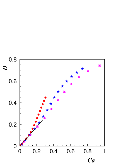
Figure 8: The deformation $D$ of the bubble as a function of the capillary number $Ca$ in a lattice of size $L=6144$ for shear rates $\dot{\gamma}\delta t=1.67\times 10^{-6}(\bullet),3.33\times 10^{-6}(\star),5.00\times 10^{-6}(\ast)$. The full line has slope $0.89$.

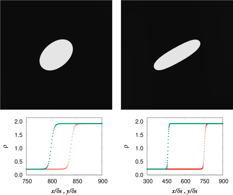
Figure 9: Density plots of the bubble (upper panels) at time $t/\delta t=5\times 10^{5}$ in a lattice of size $L=6144$ and the density profiles (lower panels) in the interface regions, plotted along the Cartesian axes $x(\bullet)$ and $y(\circ)$) centered in the middle of the flow domains, for shear rates $\dot{\gamma}\delta t=1.67\times 10^{-6}$ (left) and $5.00\times 10^{-6}$ (right). The values of the capillary number are $Ca=0.18$ (left )and $0.61$ (right).

The behavior of $D$ as a function of $Ca$ is shown in Fig. 8 for various values of the shear rate. Simulations are run until the bubble reaches the boundary. It can be seen that the deformation increases linearly with the capillary number up to $Ca\simeq 0.2$ and is independent on the value of the shear rate as previously observed chen-2010 ; chen-2011 . This can be compared with the prediction in the case of an equilibrated bubble under steady deformation for weak flows where it holds that $D=(19\lambda+16)Ca/(16\lambda+16)$ for $Ca<<1$ taylor-1932 . This would give $D\simeq 1.02Ca$ for the value $\lambda\simeq 0.12$ of our system. The best fit to numerical data gives $D\simeq 0.89Ca$. We stress that in our case the relationship between $D$ and $Ca$ is dynamic in the sense that both quantities depend on time keeping the shear rate fixed, while in the case of steady deformation $D$ is obtained by considering successive increments of $Ca$ by increasing the shear rate. When the capillary number further increases beyond $0.2$, the deformation is no longer a linear function of $Ca$ and the smaller is the shear rate the higher is the deformation with no overlap of data for the different values of the shear rate. One expects that high order contributions of $Ca$ to $D$ might be relevant also in the present problem as it is in the case of steady deformation barthes-1973 . Typical bubble conformations in the two regimes are shown in Fig. 9 at the same time for $\dot{\gamma}\delta t=1.67\times 10^{-6},5.00\times 10^{-6}$. For the lower value of $\dot{\gamma}$ it results $Ca=0.18$ so that the deformation is still linear in $Ca$ while in the other case it is $Ca=0.61$ when $D$ is no longer a linear function of the capillary number (see Fig. 8). In the same figure the finite width of the bubble interfaces along the flow and the shear directions can be appreciated with no deformation induced by the external flow. We are able to observe a non-linear regime of $D$ as a function of $Ca$ in the case of a sheared growing bubble thanks to the very large simulated system.

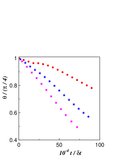
Figure 10: The tilt angle $\theta$ of the bubble as a function of time in a lattice of size $L=6144$ for shear rates $\dot{\gamma}\delta t=1.67\times 10^{-6}(\bullet),3.33\times 10^{-6}(\star),5.00\times 10^{-6}(\ast)$.

The time behavior of the tilt angle $\theta$, which is reported in Fig. 10, is observed to depend on shear rate. At the beginning the elongational component of the shear flow aligns the slightly deformed bubble along the direction of principal extension so that $\theta\simeq\pi/4$. Immediately afterward the angle diminishes and the lower is the shear rate, the higher is the tilt angle with a linear dependence of $\theta$ on the shear rate. However, at late times this dependence is no longer linear.

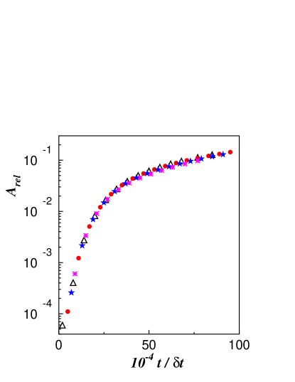
Figure 11: The fraction $A_{rel}$ of the bubble area as a function of time in a lattice of size $L=6144$ for shear rates $\dot{\gamma}\delta t=0(\triangle),1.67\times 10^{-6}(\bullet),3.33\times 10^{-6}(\star),5.00\times 10^{-6}(\ast)$.

In order to evaluate the effects of the shear on the growth rate of the bubble, the fraction $A_{rel}=N_{b}/L^{2}$ of the bubble area with respect to the system extension was computed. The results as a function of time are depicted in Fig. 11. It can be appreciated that the area of the bubble does not depend on the shear rate, even with steady walls, showing that the growth is mainly driven by the pressure difference.

Finally, we comment about the possibility of accessing larger values of the capillary number. Within the present model it is hard to go beyond $Ca\simeq 1$. Indeed, it can be noted that $Ca=\mu_{L}\dot{\gamma}\hat{R}/\sigma\simeq Ma\rho_{L}\tau T^{3/2}/\sigma$. The numerator cannot be further increased with respect to the present study since $Ma\simeq 0.5$, $\tau\lesssim 10^{-2}$ due to the constraint on the validity of the Navier-Stokes limit, and $T<T_{c}=1$. The only way would be to diminish the surface tension. Since it can be shown wagn07 that $\sigma\simeq(\rho_{L}-\rho_{V})^{2}\sqrt{\kappa(1/T-1)/2}$, one might reduce $\kappa$ and/or increase $T$ with $T<1$. However, since the interface width is proportional to $\sqrt{2\kappa/(1/T-1)}$ wagn07 , a reduction of $\kappa$ would make the interface sharper compromising the numerical stability of the method and an increase of $T$ would broaden the interface requiring larger systems to keep the same resolution thus making the simulation not feasible.

IV Conclusion

We introduced a third-order, off lattice isothermal LB model in two dimensions with the purpose to describe the growth behavior of a vapor bubble in superheated liquid. The model is based on the Gauss-Hermite quadrature and on the second-order corner transport upwind numerical scheme which is easily parallelizable as the collision-streaming LB models.

We first considered a quiescent system. We presented a corrected version of the two-dimensional Rayleigh-Plesset equation and found that our numerical results well describe the evolution of the radius of the bubble. The agreement with the solution of RP equation becomes better for larger sizes of the system. We remind that, differently from the three- dimensional case, the spatial extension of the system explicitly enters in the formulation of the RP equation in two dimensions. We also presented a careful evaluation of the critical radius of a bubble for the non-equilibrium conditions considered in this work.

Then we analyzed the same problem in presence of a shear flow imposed by external walls. We measured the growth and the deformation of the bubble induced by the flow. We expressed the deformation in terms of the dimensionless number $D$ and analyzed its dependence on the capillary number $Ca$ that is evaluated in terms of shear rate and average radius of the bubble. As expected, a linear dependence was observed at low $Ca$ but with a different proportionality coefficient than that known for bubbles in equilibrium liquids. This coefficient was found to be the same for the different shear rates considered. A non-linear regime was observed for $Ca\gtrsim 0.2$ with $D$ being slightly larger, at fixed $Ca$, for smaller shear rates. In a future research we plan to extend our method and analysis in order to control independently the viscosities of the liquid and vapor phases.

Appendix A

In order to clarify what happens with the series expansion (37) during the advection step, we first recall the definition of the tensor Hermite polynomials in the $D$-dimensional Cartesian space shan_jfm2006 :

$${\bm{\mathcal{H}}}^{(\ell)}_{\alpha_{1}\ldots\alpha_{\ell}}({\bm{\xi}})\,=\,\frac{\,(-1)^{\ell}\,}{\,\omega({\bm{\xi}})\,}\,\partial_{\xi_{\alpha_{1}}}\cdots\partial_{\xi_{\alpha_{\ell}}}\omega({\bm{\xi}})$$ (A.51)

where $\ell\in\{\,0,\,1,\,2,\,\ldots\,\}$, $\alpha_{1},\,\alpha_{2},\,\ldots\alpha_{\ell}\,\in\{\,x_{1},\,x_{2},\,\ldots\,x_{D}\,\}$ and

$$\omega({\bm{\xi}})\,=\,\frac{1}{\,(2\pi)^{D/2}\,}\,\exp(-\xi^{2}/2)\,=\,\prod_{k=1}^{D}\frac{1}{\,\sqrt{2\pi}\,}\,\exp(-\xi_{x_{k}}^{2}/2)$$ (A.52)

with

$$\xi^{2}\,=\,\sum_{k=1}^{D}\xi_{k}^{2}.$$ (A.53)

The Hermite polynomials $H^{m}(\xi_{\alpha})$ of order $m$, $m\in\{\,0,\,1,\,2,\,\ldots\,\}$, are defined on the Cartesian axis $\alpha$, in a similar way :

$$H^{m}(\xi_{\alpha})\,=\,\frac{\,(-1)^{m}\,}{\,\omega(\xi_{\alpha})\,}\,\partial_{\xi_{\alpha}}^{m}\omega(\xi_{\alpha})$$ (A.54)

and satisfy the recurrence relation

$$\xi_{\alpha}H^{(m)}(\xi_{\alpha})\,=\,H^{(m+1)}(\xi_{\alpha})\,+\,m\,H^{(m-1)}(\xi_{\alpha})$$ (A.55)

In the two-dimensional space, we have $D=2$ and $x_{1}\equiv x$ , $x_{2}\equiv y$. We use the Kronecker symbol $\delta_{\alpha\beta}$ to write:

$$\partial_{\xi_{\alpha}}\,=\,\delta_{\alpha x}\partial_{\xi_{x}}+\delta_{\alpha y}\partial_{\xi_{y}}.$$ (A.56)

This allows us to express the tensor Hermite polynomials ${\bm{\mathcal{H}}}^{(\ell)}_{\alpha_{1}\ldots\alpha_{\ell}}({\bm{\xi}})$ with respect to the Hermite polynomials $H^{m}(\xi_{\alpha})$ :

$${\bm{\mathcal{H}}}^{(\ell)}_{\alpha_{1}\ldots\alpha_{\ell}}({\bm{\xi}}) = \frac{\,(-1)^{\ell}\,}{\,\omega({\bm{\xi}})\,}\,\prod_{k=1}^{\ell}(\delta_{\alpha_{k}x}\partial_{\xi_{x}}+\delta_{\alpha_{k}y}\partial_{\xi_{y}})\,\omega({\bm{\xi}})$$ (A.59)

$$= \sum_{{\tiny{\begin{array}[]{c}m,n=0\\ m+n=\ell\end{array}}}}^{\ell}\,\delta_{(m,n)}^{(\ell)}\,\left[\,\frac{\,(-1)^{m}\,}{\,\omega(\xi_{x})\,}\,\partial_{\xi_{x}}\omega(\xi_{x})\,\right]\,\left[\frac{\,(-1)^{n}\,}{\,\omega(\xi_{y})\,}\,\partial{\xi_{y}}\omega(\xi_{y})\,\right]$$

$$= \sum_{{\tiny{\begin{array}[]{c}m,n=0\\ m+n=\ell\end{array}}}}^{\ell}\,\delta_{(m,n)}^{(\ell)}\,H^{m}(\xi_{x})H^{n}(\xi_{y})$$ (A.62)

where the symbol $\delta_{(m,n)}^{(\ell)}$, with $m+n=\ell$, is defined recursively, as follows. For $\ell=m=n=0$, we set

$$\delta_{(0,0)}^{(0)}\,=\,1.$$ (A.63)

For $\ell>0$, when $m=\ell$ or $n=\ell$, we define

$$\delta_{(\ell,0)}^{(\ell)} = \delta_{(\ell-1,0)}^{(\ell-1)}\delta_{\alpha_{l}x}$$ (A.64)

$$\delta_{(0,\ell)}^{(\ell)} = \delta_{(0,\ell-1)}^{(\ell-1)}\delta_{\alpha_{l}y}\rule{0.0pt}{19.91692pt}$$ (A.65)

and, for $\ell,m,n>0$, $m+n=\ell$ :

$$\delta_{(m,n)}^{(\ell)}\,=\,\delta_{(m-1,n)}^{(\ell-1)}\delta_{\alpha_{l}x}\,+\,\delta_{(m,n-1)}^{(\ell-1)}\delta_{\alpha_{l}y}.$$ (A.66)

In this way we are able to get the expansion of the tensor Hermite polynomials up to order $N=4$ with respect to the Hermite polynomials:

$${\bm{\mathcal{H}}}^{(0)}({\bm{\xi}}) = H^{(0)}(\xi_{x})H^{(0)}(\xi_{y}),$$ (A.67)

$${\bm{\mathcal{H}}}^{(1)}_{\alpha}({\bm{\xi}}) = \delta_{\alpha x}H^{(1)}(\xi_{x})H^{(0)}(\xi_{y})\,+\,\delta_{\alpha y}H^{(0)}(\xi_{x})H^{(1)}(\xi_{y}),\rule{0.0pt}{19.91692pt}$$ (A.68)

$${\bm{\mathcal{H}}}^{(2)}_{\alpha\beta}({\bm{\xi}}) = \delta_{\alpha x}\delta_{\beta x}H^{(2)}(\xi_{x})H^{(0)}(\xi_{y})\rule{0.0pt}{19.91692pt}$$ (A.69)

$$+ (\delta_{\alpha x}\delta_{\beta y}\,+\,\delta_{\alpha y}\delta_{\beta x})H^{(1)}(\xi_{x})H^{(1)}(\xi_{y})\rule{0.0pt}{19.91692pt}$$

$$+ \delta_{\alpha y}\delta_{\beta y}H^{(0)}(\xi_{x})H^{(2)}(\xi_{y}),\rule{0.0pt}{19.91692pt}$$

$${\bm{\mathcal{H}}}^{(3)}_{\alpha\beta\gamma}({\bm{\xi}}) = \delta_{\alpha x}\delta_{\beta x}\delta_{\gamma x}H^{(3)}(\xi_{x})H^{(0)}(\xi_{y})\rule{0.0pt}{19.91692pt}$$ (A.70)

$$+ (\delta_{\alpha x}\delta_{\beta x}\delta_{\gamma y}\,+\,\delta_{\alpha x}\delta_{\beta y}\delta_{\gamma x}\,+\,\delta_{\alpha y}\delta_{\beta x}\delta_{\gamma x})\,H^{(2)}(\xi_{x})H^{(1)}(\xi_{y})\rule{0.0pt}{19.91692pt}$$

$$+ (\delta_{\alpha y}\delta_{\beta y}\delta_{\gamma x}\,+\,\delta_{\alpha y}\delta_{\beta x}\delta_{\gamma y}\,+\,\delta_{\alpha x}\delta_{\beta y}\delta_{\gamma y})\,H^{(1)}(\xi_{x})H^{(2)}(\xi_{y})\rule{0.0pt}{19.91692pt}$$

$$+ \delta_{\alpha y}\delta_{\beta y}\delta_{\gamma y}\,H^{(0)}(\xi_{x})H^{(3)}(\xi_{y})\rule{0.0pt}{19.91692pt},$$

$${\bm{\mathcal{H}}}^{(4)}_{\alpha\beta\gamma\sigma}({\bm{\xi}}) = \delta_{\alpha x}\delta_{\beta x}\delta_{\gamma x}\delta_{\sigma x}\,H^{(4)}(\xi_{x})H^{(0)}(\xi_{y})\rule{0.0pt}{19.91692pt}$$ (A.71)

$$+ (\delta_{\alpha x}\delta_{\beta x}\delta_{\gamma x}\delta_{\sigma y}\,+\,\delta_{\alpha x}\delta_{\beta x}\delta_{\gamma y}\delta_{\sigma x}\,+\,\delta_{\alpha x}\delta_{\beta y}\delta_{\gamma x}\delta_{\sigma x}\,+\,\rule{0.0pt}{19.91692pt}$$

$$\,\,\delta_{\alpha y}\delta_{\beta x}\delta_{\gamma x}\delta_{\sigma x})\,H^{(3)}(\xi_{x})H^{(1)}(\xi_{y})\rule{0.0pt}{19.91692pt}$$

$$+ (\delta_{\alpha x}\delta_{\beta x}\delta_{\gamma y}\delta_{\sigma y}\,+\,\delta_{\alpha x}\delta_{\beta y}\delta_{\gamma x}\delta_{\sigma y}\,+\,\delta_{\alpha y}\delta_{\beta x}\delta_{\gamma x}\delta_{\sigma y}\,+\,\rule{0.0pt}{19.91692pt}$$

$$\,\,\delta_{\alpha x}\delta_{\beta y}\delta_{\gamma y}\delta_{\sigma x}\,+\,\delta_{\alpha y}\delta_{\beta x}\delta_{\gamma y}\delta_{\sigma x}\,+\,\delta_{\alpha y}\delta_{\beta y}\delta_{\gamma x}\delta_{\sigma x})\,H^{(2)}(\xi_{x})H^{(2)}(\xi_{y})\rule{0.0pt}{19.91692pt}$$

$$+ (\delta_{\alpha y}\delta_{\beta y}\delta_{\gamma y}\delta_{\sigma x}\,+\,\delta_{\alpha y}\delta_{\beta y}\delta_{\gamma x}\delta_{\sigma y}\,+\,\delta_{\alpha y}\delta_{\beta x}\delta_{\gamma y}\delta_{\sigma y}\,+\,\rule{0.0pt}{19.91692pt}$$

$$\,\,\delta_{\alpha x}\delta_{\beta y}\delta_{\gamma y}\delta_{\sigma y})\,H^{(0)}(\xi_{x})H^{(3)}(\xi_{y})\rule{0.0pt}{19.91692pt}$$

$$+ \delta_{\alpha y}\delta_{\beta y}\delta_{\gamma y}\delta_{\sigma y}\,H^{(0)}(\xi_{x})H^{(4)}(\xi_{y}).\rule{0.0pt}{19.91692pt}$$

Table 4: $(m,n)$ pairs in the expansion (A.62) of the function $f_{k}$ (see the text for further details).

[0,4]		[1,4]		[2,4]		[3,4]		[4,4]
(0,3)		(1,3)		(2,3)		(3,3)		[4,3]
(0,2)		(1,2)		(2,2)		(3,2)		[4,2]
(0,1)		(1,1)		(2,1)		(3,1)		[4,1]
(0,0)		(1,0)		(2,0)		(3,0)		[4,0]

In our LB model (of order $N=3$), the Cartesian components of the discrete velocity vectors are roots of the Hermite polynomial of order $Q=N+1=4$. Let us assume that at time $t=0$, the distribution function $f_{k}$, $k=1,\,2,\,\ldots K$, is expressed as an expansion up to order $N=3$ with respect to the tensor Hermite polynomials, Eq. (37). According to Eq. (A.62), this means that $f_{k}$ contains all the terms $H^{(m)}(\xi_{x})H^{(n)}(\xi_{y})$, with $0\leq m+n\leq 3$, marked in black as $(m,n)$ in the lower left corner of Table 4. After performing a time step $\delta t$, the expansion of $f_{k}$ will include five new terms, namely the tensor Hermite polynomials of order $\ell=4$, in accordance to the recurrence relation (38). According to the recurrence relation for Hermite polynomials (A.55), these new terms of order 4 (marked in red color on the north-west – south-east diagonal on Table 4) are of the type $H^{(m)}(\xi_{x})H^{(n)}(\xi_{y})$, with $m+n=4$. Two of these terms, namely $H^{(4)}(\xi_{x})H^{(0)}(\xi_{y})$ and $H^{(0)}(\xi_{x})H^{(4)}(\xi_{y})$, vanish because the components of the velocity vectors used in this models are roots of the Hermite polynomials of order N=4. The indices $m,n$ corresponding to these particular ”red color” terms are evidenced by square brackets (i.e., $[4,0]$ and $[0,4])$ in Table 4. At the next time step, the remaining (non-vanishing) red terms of order $\ell=m+n=4$ evolve further and produce the green terms in the table. Subsequent time steps produce the terms marked cyan and magenta. Since $H^{(m)}(\xi_{x})H^{(n)}(\xi_{y})=0$ for $m=4$ or $n=4$, the subsequent time steps never produce non-vanishing terms of order $m+n>2N$ in the expression of $f_{k}$.

Figure 4: Liquid- vapor phase diagram: Symbols refer to LB results on the liquid branch ($\blacksquare$) and on the vapor one ($\bullet$). The full lines correspond to the results of the Maxwell construction.

References

- (1) J. M. Rallison, Annu. Rev. Fluid Mech. 16, 45 (1984).
- (2) C. E. Brennen, Cavitation and Bubble Dynamics, (Oxford University, New York, 1995).
- (3) M. Plesset, J. Fluid Eng. 85, 360 (1963).
- (4) H. J. de Vega, I. M. Khalatnikov, and N. G. Sanchez, eds., Phase Transitions in the Early Universe: Theory and Observations, (Springer, Berlin, 2001).
- (5) H. Massol and T. Koyaguchi, J. Volcanol. Geotherm. Res. 143, 69 (2005).
- (6) A. Y. Kuksin, G. E. Norman, V. V. Pisarev, V. V. Stegailov, and A. V. Yanilkin, Phys. Rev. B 82, 174101 (2010).
- (7) H. Watanabe, M. Suzuki, and N. Ito, Phys. Rev. E 82, 051604 (2010).
- (8) J. Diemand, R. Angelil, K. K. Tanaka, and H. Tanaka, Phys. Rev. E 90, 052407 (2014).
- (9) R. Angelil, J. Diemand, K. K. Tanaka, and H. Tanaka, Phys. Rev. E 90, 063301 (2014).
- (10) M. C. Sukop and D. Or, Phys. Rev. E 71, 046703 (2005).
- (11) X.-P. Chen, Commun. Comput. Phys. 7, 212 (2010).
- (12) X.-P. Chen, C.-W. Zhong, and X.-L. Yuan, Comput. Math. Appl. 61, 3577 (2011).
- (13) M. Zhong, C. Zhong, and C. Bai, Adv. Comput. Sci. Appls 1, 73 (2012).
- (14) For a review, see for example, Z. C. Feng and L. G. Leal, Annu. Rev. Fluid Mech. 29, 201 (1997).
- (15) L. Rayleigh, Philos. Mag. 34 (1917).
- (16) M. Plesset, J. Appl. Mech. 16, 277 (1949).
- (17) M. S. Plesset and A. Prosperetti, Annu. Rev. Fluid Mech. 9, 145 (1977); A. Prosperetti and M. S. Plesset, J. Fluid Mech. 85, 349 (1978).
- (18) S. Chen, G.D. Doolen, Annu. Rev. Fluid. Mech. 30 (1998) 329.
- (19) S. Succi, The Lattice Boltzmann Equation for Fluid Dynamics and Beyond, (Clarendon Press, Oxford, 2001).
- (20) M.C. Sukop, D.T. Thorne, Lattice Boltzmann Modeling: An Introduction for Geoscientists and Engineers, (Springer, Berlin, 2006).
- (21) C. K. Aidun and J. R. Clausen, Annu. Rev. Fluid. Mech. 42 (2010) 439.
- (22) Z. Guo, C. Shu, Lattice Boltzmann Method and its Applications in Engineering, (World Scientific, Singapore, 2013).
- (23) H.B. Huang, M.C. Sukop, X.Y. Lu, Multiphase Lattice Boltzmann Methods: Theory and Application, Wiley Blackwell, Chichester, 2015
- (24) T. Krüger, H. Kusumaatmaja, A. Kuzmin, O. Shardt, G. Silva, E.M. Viggen, The Lattice Boltzmann Method Principles and Practice, (Springer, London, 2017).
- (25) X. Shan, X. Yuan, H. Chen, J. Fluid. Mech 550 (2006) 413.
- (26) N. Cao, S. Chen, S. Jin, D. Martinez, Phys. Rev. E 55 (1997) R21.
- (27) T. Biciuşcă, A. Horga, V. Sofonea, Comptes Rendus Mécanique 343, 580 (2015).
- (28) P. Yuan and L. Schaefer, Phys. Fluids 18, 042101 (2006).
- (29) For a review see, e. g., L. Chen, Q. Kang, Y. Mu, Y.-L. He, and W.-Q. Tao, Int. J. Heat and Mass Transfer 76, 210 (2014).
- (30) G. Kähler, F. Bonelli, G. Gonnella, and A. Lamura, Phys. Fluids 27, 123307 (2015).
- (31) S. Richardson, J. Fluid Mech. 33, 476 (1968).
- (32) J. D. Buckmaster and J. E. Flaherty, J. Fluid Mech. 60, 625 (1973).
- (33) I. Halliday and C. M. Care, Phys. Rev. E 53, 1602 (1996).
- (34) I. Halliday, C. M. Care, S. Thompson, and D. White, Phys. Rev. E 54, 2573 (1996).
- (35) A. J. Wagner and J. M. Yeomans, Int. J. Mod. Phys. C 8, 773 (1997).
- (36) P. Colella, J. Comput. Phys. 87 (1990) 171.
- (37) R.J. Leveque, SIAM J. Numer. Anal. 33, 627 (1996).
- (38) R.J. Leveque, Finite Volume Methods for Hyperbolic Problems, (Cambridge University Press, Cambridge, 2001).
- (39) J.A. Trangenstein, Numerical Solution of Hyperbolic Partial Differential Equations, (Cambridge University Press, Cambridge, 2009).
- (40) T. Laurila, A. Carlson, M. Do-Quang, T. Ala-Nissila, and G. Amberg, Phys. Rev. E 85, 026320 (2012).
- (41) G. Falcucci, E. Jannelli, S. Ubertini, and S. Succi J. Fluid Mech. 728, 362 (2013).
- (42) V. Sofonea, A. Lamura, G. Gonnella, and A. Cristea, Phys. Rev. E 70 (2004) 046702; A. Cristea, G. Gonnella, A. Lamura, and V. Sofonea, Math. Comput. Simulat. 72, 113 (2006).
- (43) V.E. Ambruş and V. Sofonea, Phys. Rev. E 86 (2012) 016708.
- (44) V.E. Ambruş and V. Sofonea, J. Comput. Phys. 316 (2016) 760.
- (45) X. Shan and X. He, Phys. Rev. Lett. 80 (1998) 65.
- (46) B. Piaud, S. Blanco, R. Fournier, V.E. Ambrus, and V. Sofonea, Int. J. Mod. Phys. C 25 (2014) 1340016.
- (47) F.B. Hildebrandt, Introduction to Numerical Analysis (second edition), (Dover Publications, 1987).
- (48) B. Shizgal, Spectral Methods in Chemistry and Physics: Applications to Kinetic Theory and Quantum Mechanics, (Springer, 2015).
- (49) X. Shan, Phys. Rev. 77 (2008) 066702.
- (50) K. Suga, Fluid. Dyn. Res. 45 (2013) 034501.
- (51) X. Niu, S. Hyodo, T. Munekata, Phys. Rev. E 76 (2007) 036711.
- (52) K. Suga, S. Takenaka, T. Ito, M. Kaneda, T. Kinjo, S. Hyodo, Phys. Rev. E 82 (2010) 016701.
- (53) S. Ansumali, I.V. Karlin, H.C. Öttinger, Europhys. Lett. 63 (2003) 798.
- (54) A. Bardow, I.V. Karlin, A.A. Gusev, Europhys. Lett. 75 (2006) 434.
- (55) A. Bardow, I.V. Karlin, A.A. Gusev, Phys. Rev. E 77 (2008) 025701(R).
- (56) L.S. Luo, Phys. Rev. Lett. 81 (1998) 1618.
- (57) L.S. Luo, Phys. Rev. E 62 (2000) 4982.
- (58) A. Cristea, G. Gonnella, A. Lamura, and V. Sofonea, Commun. Comput. Phys. 7 (2010) 350.
- (59) A. Coclite, G. Gonnella, and A. Lamura, Phys. Rev. E 89, 063303 (2014).
- (60) J. S. Rowlinson and B. Widom, Molecular Theory of Capillarity, (Clarendon Press, Oxford, 1982).
- (61) R. Evans, Adv. Phys. 28, 143 (1979).
- (62) G. Gonnella, A. Lamura, and V. Sofonea, Phys. Rev. E 76, 036703 (2007); G. Gonnella, A. Lamura, and V. Sofonea, Eur. Phys. J. - Spec. Top. 171, 181 (2009).
- (63) Y.L. Klimontovich, Kinetic Theory of Nonideal Gases and Nonideal Plasmas, (Pergamon Press, Oxford, 1982).
- (64) S.Leclaire, M. El-Hachem, J.Y.Trepanier, and M.Reggio, J. Sci. Comput. 59 (2014) 545.
- (65) M. Patra and M.Karttunen, Numer. Methods Partial Differ. Eqs. 22 (2006) 936.
- (66) K.K.Mattila, L.A.Hegele, and P.C.Philippi, Sci. World J. 2014 (2014) 142907.
- (67) D. N. Siebert, P. C. Philippi, and K. K. Mattila, Phys. Rev. E 90 (2014) 053310.
- (68) R. Farber, CUDA Application Design and Development, *Morgan Kaufmann, Waltham, MA, 2011).
- (69) S. Cook, CUDA Programming, A developer’s Guide to Parallel Computing with GPUs, (Morgan Kaufmann, Waltham, MA, 2013).
- (70) J. Cheng, M. Grossman, and T. McKercher, Professional CUDA C Programming, John Wiley and Sons, Inc., Indianapolis, IN, 2014.
- (71) CUDA C Programming Guide, http://docs.nvidia.com/cuda/pdf/CUDA_C_Programming_Guide.pdf.
- (72) M.O. Deville and T.B. Gatski, Mathematical Modeling for Complex Fluids and Flows, (Springer, Berlin, 2012).
- (73) P.C. Philippi, L.A. Hegele Jr., L.O.E. dos Santos, and R. Surmas, Phys. Rev. E 73 (2006) 056702.
- (74) D.N. Siebert, L.A. Hegele Jr., and P.C. Philippi, Phys. Rev. E 77 (2008) 026707.
- (75) R. Surmas, C.E. Pico Ortiz, and P.C. Philippi, Eur. Phys. J. Special Topics 171 (2009) 81.
- (76) S.S. Chikatamarla and I.V. Karlin, Phys. Rev. E 79 (2009) 046701.
- (77) W.P. Yudistiawan, S. Ansumali, and I.V. Karlin, Phys. Rev. E 78 (2008) 016705.
- (78) W.P. Yudistiawan, S.K. Kwak, D.V. Patil, and S. Ansumali, Phys. Rev. E 82 (2010) 046701.
- (79) X.Y. He, Int. J. Mod. Phys. C 8 (1997) 737.
- (80) X.D. Niu, C. Shu, Y.T. Chew, and T.G. Wang, J. Stat. Phys. 117 (2004) 665.
- (81) V. Sofonea, J. Comput. Phys. 228 (2009) 6107.
- (82) S. Ubertini, S. Succi, Commun. Comput. phys. 3 (2008) 342.
- (83) Z. Guo, T.S. Zhao, Phys. Rev. E 67 (2003) 066709.
- (84) T. Lee, C.L. Lin, J. Comput. Phys. 171 (2001) 336.
- (85) T. Lee, C.L. Lin, J. Comput. Phys. 185 (2003) 445.
- (86) K. Hejranfar, E. Ezzatneshan, Phys. Rev. E 92 (2015) 053305.
- (87) D.M. Bond, W. Wheatley, M.N. Macrossan, and M. Goldsworthy, J. Comput. Phys 259 (2014) 175.
- (88) F. Nannelli and S. Succi, J. Stat. Phys. 68 (1992) 401.
- (89) H. Chen, Phys. Rev. E 58 (1998) 3955.
- (90) R. Zhang, H. Chen, Y. Qian, and S. Chen, Phys. Rev. E 63 (2001) 056705.
- (91) M. Sbragaglia and K. Sugiyama, Phys. Rev. E 82 (2010) 046709.
- (92) V. Sofonea, R. F. Sekerka, J. Comput. Phys. 184 (2003) 422.
- (93) A.Cristea, V.Sofonea, Cent. Eur. J. Phys. 2, 382 (2004).
- (94) R. Zhang, X. Shan, H. Chen, Phys. Rev. E 74 (2006) 046703.
- (95) A. Sescu, R. Hixon, J. Sci. Comput. 61 (2014) 327.
- (96) A. Sescu, Adv. Differ. Equ. 2015 (2015) 9.
- (97) J. Latt, B. Chopard, Math. Comput. Simulat. 72 (2006) 165.
- (98) C. Colosqui, H. Chen, X. Shan, I. Staroselsky, Phys. Fluids 21 (2009) 013105.
- (99) C. Colosqui, Phys. Rev. E 81 (2010) 026702.
- (100) A. Montessori, G. Falcucci, P. Prestininzi, M. La Rocca, S. Succi, Phys. Rev. E 89 (2015) 053317.
- (101) K. K. Mattila, P. C. Philippi, L. A. Hegele, Jr., Phys. Fluids 29 (2017) 046103.
- (102) P. Fede, V. Sofonea, R. Fournier, S. Blanco, O. Simonin, G. Lepoutère, and V. Ambruş, Int. J. Multiphase Flow 76 (2015) 187.
- (103) V. Sofonea and R.F. Sekerka, Phys. Rev. E 71 (2005) 066709.
- (104) V.E. Ambruş and V. Sofonea, Phys. Rev. E 89 (2014) 041301(R).
- (105) Y. Sone Molecular Gas Dynamics : Theory, Techniques and Applications (Birkhäuser, Boston, 2007).
- (106) G. Karniadakis, A. Beşkok, N. Aluru, Microflows and Nanoflows: Fundamentals and Simulation (Springer, Berlin, 2005).
- (107) A. Acrivos, Ann. NY Acad. Sci. 404, 1 (1983); H. A. Stone, Annu. Rev. Fluid Mech. 26, 65 (1994).
- (108) X. B. Nie, X. Shan, and H. Chen, EPL 81, 34005 (2008).
- (109) G. I. Taylor, Proc. R. Soc. A 138, 41 (1932).
- (110) D. Barthès-Biesel and A. Acrivos, J. Fluid Mech. 61, 1 (1973).
- (111) A. J. Wagner and C. M. Pooley, Phys. Rev. E 76, 045702(R) (2007).