Optical orientation and alignment of excitons in ensembles of inorganic perovskite nanocrystals

Abstract

We demonstrate the optical orientation and alignment of excitons in a two-dimensional layer of CsPbI₃ perovskite nanocrystals prepared by colloidal synthesis and measure the anisotropic exchange splitting of exciton levels in the nanocrystals. From the experimental data at low temperature (2 K), we obtain the average value of anisotropic splitting of bright exciton states of the order of 120 $\mu$eV. Our calculations demonstrate that there is a significant contribution to the splitting due to the nanocrystal shape anisotropy for all inorganic perovskite nanocrystrals.

I Introduction

Hybrid organic-inorganic halide perovskites are new optoelectronic materials that have attracted enormous attention as solution-deposited absorbing layers in solar cells with power conversion efficiencies of above 20%.Green et al. (2014); Sum and Mathews The excellent optoelectronic properties of organic halide perovskite thin films are comparable to those of conventional direct-gap semiconductors like GaAs, which makes the perovskites promising for generating and detecting spin.Zhang et al. (2015) The potential of halide perovskites for spintronic applications is just beginning to be investigated.Odenthal et al. (2017)

While all-inorganic Cs–Pb-halide perovskite nanocrystals (NCs), fabricated via colloidal synthesis, have been introduced only recently,Protesescu et al. (2015) they have already greatly impressed the scientific community by their unprecedented brightness and abnormally high photoemission rates. This shows good promise for a range of applications from color-converting phosphors and light-emitting diodesTan et al. (2014) to lasers.Xing et al. (2014); Yakunin et al. (2015) Various spectroscopic techniques and theoretical considerations have been applied to conduct a comprehensive study of spectral and dynamical characteristics of single- and multi-exciton states in CsPbX₃ NCs with X being either Br, I, or their mixture.Makarov et al. (2016); Lin et al. (2016); de Weerd et al. (2016); de Jong et al. (2017); Becker et al. (2018)

The fine structure of exciton levels in CsPbBr₃Fu et al. (2017) and CsPbI₃Yin et al. (2017) NCs has been probed by means of the single-dot spectroscopy. Splittings of the bright exciton level into linearly polarized components were detected which were on the order of $1$ meV for CsPbBr₃ NCs and several hundred $\mu$eV for CsPbI₃ NCs with the mean size of $\sim$ $10$ nm. However, Yin et al. emphasized that, for some samples, the fine structure splittings for all NCs were below their spectral resolution of $200$ $\mu$eV, although the same synthesis procedure was nominally adopted.Yin et al. (2017) Switching of the NC emission from the split exciton line to a single red-shifted trion line was also observed in these experiments when the photoexcitation power was above a certain threshold.Fu et al. (2017); Yin et al. (2017) Recently ensemble measurements of magneto-photoluminescence have been undertaken for CsPbBr₃ NCs(Canneson et al., 2017) and 90% of photoluminescence was attributed to negatively charged trions, though excitation power density did not exceed $1$ W/cm².Canneson et al. (2017)

In this work we investigate optical orientation and alignment of excitons in ensembles of CsPbI₃ NCs. Our experimental approach has been previously used to probe the fine structure of excitons in bulk III-V and II-VI semiconductorsPikus and Ivchenko (1982); Planel and Benoit a la Guillaume (1984) and heterostructuresIvchenko (1995); Ivchenko and Pikus (2095) with quantum wells, quantum dots,Dzhioev et al. (1997a, b, 1998a, 1998b) and quantum wires.Dzhioev et al. (2003) This technique allows one to measure a splitting of bright exciton levels averaged over an ensemble. This technique is not limited by the spectral resolution and allows one to measure splittings as low as few $\mu$eV. It also allows to study the ensembles in situ with account on possible interaction between the NCs.Lin et al. (2016)

In our samples containing a two-dimensional layer of CsPbI₃ NCs, the suppression of the optical orientation at zero magnetic field, together with the strong optical alignment of photoexcitations, indicates that photoluminescence (PL) is dominated by the neutral excitons. The dependence of the degree of the photoluminescence linear polarization on the magnetic field allowed us to measure the ensemble-averaged splitting between linearly polarized components of the bright exciton state of 120 $\mu$eV.

The paper is organized as follows. In Sec. II we briefly review what is known on the crystal structure and the electronic band structure of inorganic perovskites. A comprehensive theoretical analysis of the origin of the bright exciton level splitting is presented in Sec. III. We also estimate the splitting caused by the NCs shape anisotropy from the ${\bm{k}}\cdot{\bm{p}}$ analysis. The details of sample synthesis and experimental measurements are presented in Secs. IV and V, respectively. In Sec. VI we discuss experimental results which enable us to extract the value of the ensemble-averaged splitting between linearly polarized components of the bright exciton state. In Sec. VII we discuss the origin of this splitting. In Sec. VIII the conclusions are drawn.

II Bandstructure of inorganic halide perovskites

The inorganic perovskites CsPbI₃, as well as other bulk APbX₃ perovskite materials, are known to form at least three different phases:Møller (1958); Fujii et al. (1974); Fu et al. (2017) the high-temperature cubic phase ($O_{h}$ point group), the tetragonal phase ($D_{4h}$), and the low-temperature orthorhombic phase ($D_{2h}$). There exist reports of yet another low-temperature, monoclinic phase.Fujii et al. (1974) All phase transitions in the bulk perovskites occur well above room temperature.Møller (1958); Fujii et al. (1974) In ultrathin two-dimensional CsPbBr₃ halide perovskites, the coexistence of different phases at room temperature has been observed.Yu et al. (2016) For NCs, the phase transition temperatures may be strongly shifted by the presence of the surfaceHaruyama et al. (2016); Murali et al. (2016); Wang et al. (2017) and the synthesis method proposed in Ref. Protesescu et al., 2015 leads to all CsPbX₃ NCs crystallization in the cubic phase.Protesescu et al. (2015) Fu et al.Fu et al. (2017) and Yin et al.Yin et al. (2017), basing on X-ray diffraction measurements, also reported cubic crystal structure of CsPbBr₃ and CsPbI₃ NCs, respectively, at room temperature. However, recent comparison of the X-ray diffraction spectra of CsPbBr₃ NCs with the calculated pair distribution function allowed Cottingham and BrutcheyCottingham and Brutchey (2016) to conclude that the room-temperature crystal structure of these NCs is orthorhombic.

A detailed analysis of the perovskites symmetry can be found in the literature.Even et al. (2015); Even (2015); Yu (2016) Most of the basic properties of inorganic halide perovskites may be understood from an analysis of the cubic phase. In this phase crystals have the point group $O_{h}$ coinciding with the group of the wave vector at the $R$ point of the Brillouin zone, where the band extrema are located. The conduction and valence bands of lead halide perovskites arise from the cationic $p$ and $s$ orbitals, respectively, i.e. the band ordering is reversed as compared to classical semiconductors. Near the $R$ point the structure of the conduction band can be described by the effective Hamiltonian

$$\hat{H}({\bf k})=\hat{H}_{0}({\bf k})+\hat{H}_{SO}\,,$$ (1)

where

$$\hat{H}_{0}({\bf k})=-A\,k^{2}+3\,B\sum\limits_{\alpha}\hat{J}_{\alpha}^{2}\left(k_{\alpha}^{2}-{k^{2}}/{3}\right)\\ +2\,\sqrt{3}\,D\,\sum\limits_{\alpha>\beta}\left\{\hat{J}_{\alpha}\hat{J}_{\beta}\right\}_{s}\,k_{\alpha}\,k_{\beta}\,,$$ (2)

$$\hat{H}_{SO}=\frac{\Delta}{3}\,\sum_{\alpha}\hat{J}_{\alpha}\hat{\sigma}_{\alpha}\,,$$ (3)

$A$, $B$, and $D$ are the conduction band parameters, $\alpha,\beta=x,y,z$, $\hat{J}_{\alpha}$ are the matrices of the angular momentum $j=1$, $\hat{\sigma}_{\alpha}$ are the Pauli matrices, $\Delta$ is the spin-orbit splitting of the conduction band, and $\left\{\hat{J}_{\alpha}\hat{J}_{\beta}\right\}_{s}=\left(\hat{J}_{\alpha}\hat{J}_{\beta}+\hat{J}_{\beta}\hat{J}_{\alpha}\right)/2$.

The band structure of the low symmetry phases may be considered as the folded band structure of the cubic phase, with the small effect of symmetry reduction.Even et al. (2015) The electronic states in the vicinity of the band gap are folded from the $R$ point of the Brillouin zone onto the $\Gamma$ point and the crystal field splitting is added.

The tetragonal ($D_{4h}$) phase is characterized by the crystal field splitting described by

$$\hat{H}_{CF}^{(1)}=\epsilon_{1}\,\left[\hat{J_{z}}^{2}-{2}/{3}\right]\,,$$ (4)

while the orthorhombic ($D_{2h}$) phase is associated with additional crystal field splitting of the form

$$\hat{H}_{CF}^{(2)}=\epsilon_{2}\,\left[\hat{J_{y}}^{2}-\hat{J_{x}}^{2}\right]\,.$$ (5)

For the $D_{4h}$ case ($\epsilon_{2}=0$), the resulting Hamiltonian can be diagonalized at $k=0$. In particular, this yields the basis Bloch wave functions for the irreducible representation $\Gamma_{6}^{-}$ of the group $D_{4h}$ which corresponds to the lowest conduction band. They are

$$|\Gamma_{6}^{-},\uparrow\rangle=\frac{\cos{\xi}}{\sqrt{2}}\,(X+i\,Y)\,\downarrow+\sin{\xi}\,Z\,\uparrow\,,$$ (6)

$$|\Gamma_{6}^{-},\downarrow\rangle=\frac{\cos{\xi}}{\sqrt{2}}\,(X-i\,Y)\,\uparrow-\sin{\xi}\,Z\,\downarrow\,,$$ (7)

where $\tan{2\xi}=\frac{2\sqrt{2}\Delta}{\Delta-3\,\epsilon_{1}}$. The phases of these functions are chosen to yield the basis functions of the representation $\Gamma_{7}$ of the group $T_{d}$ (analogous to the representation $\Gamma_{6}^{-}$ of the group $O_{h}$) in the limit $\epsilon_{1}=0$.Ivchenko (2005) These functions, along with the valence-band wave functions,

$$|\Gamma_{6}^{+},\uparrow\rangle=S\,\uparrow\,,$$ (8)

$$|\Gamma_{6}^{+},\downarrow\rangle=S\,\downarrow\,,$$ (9)

will be used in Sec. III.2 to obtain the matrix element of the long-range electron-hole exchange interaction.

III Fine structure of exciton levels

For an exciton in a crystal with point group $O_{h}$, formed by the electron from the $\Gamma_{6}^{-}$ band and the hole from the $\Gamma_{6}^{+}$ band, the isotropic part of the electron-hole exchange interaction splits the fourfold degenerate exciton level into an optically inactive singlet of $\Gamma_{1}^{-}$ symmetry $\left|0,0\right\rangle$ and optically active triplet of $\Gamma_{4}^{-}$ symmetry $\left|1,xyz\right\rangle$ (Fig. 1). A reduction of symmetry due to anisotropy of NC shape or lowering of the crystal symmetry to $D_{4h}$ allows for the splitting of the bright exciton level into the “in-plane” doublet and the $\Gamma_{2}^{-}$ optically active singlet. For $D_{2h}$ point symmetry, all excitonic levels are non-degenerate.

$\begin{matrix}\left|0,0\right\rangle=&\phantom{-}{\color[rgb]{0,0,1}\uparrow}{\color[rgb]{1,0,0}\downarrow}-\phantom{i}{\color[rgb]{0,0,1}\downarrow}{\color[rgb]{1,0,0}\uparrow}\\ \hline\cr\left|1,x\right\rangle=&-{\color[rgb]{0,0,1}\uparrow}{\color[rgb]{1,0,0}\uparrow}-i{\color[rgb]{0,0,1}\downarrow}{\color[rgb]{1,0,0}\downarrow}\\ \left|1,y\right\rangle=&\phantom{-}{\color[rgb]{0,0,1}\uparrow}{\color[rgb]{1,0,0}\uparrow}-i{\color[rgb]{0,0,1}\downarrow}{\color[rgb]{1,0,0}\downarrow}\\ \left|1,z\right\rangle=&\phantom{-}{\color[rgb]{0,0,1}\uparrow}{\color[rgb]{1,0,0}\downarrow}+\phantom{i}{\color[rgb]{0,0,1}\downarrow}{\color[rgb]{1,0,0}\uparrow}\end{matrix}$

Figure 1: Qualitative scheme of the exchange splitting of bright exciton triplet state $|1,xyz\rangle$ for different symmetries of the NC. The actual order of split levels may be different.

In a NC of highly anisotropic shape, even when the crystal structure is cubic, the symmetry allows for the full splitting of the bright excitonic level into the $\left|x\right\rangle$, $\left|y\right\rangle$, and $\left|z\right\rangle$ states. Below we use optical orientation measurements to extract information about the fine structure of the bright exciton states in NCs of CsPbI₃. The fine structure of the bright exciton is defined by the exchange interaction between the electron and the hole. Microscopically, the exchange splitting may be considered as the sum of two contributions: the long-range (non-analytic) and the short-range (analytic).Bir and Pikus (1974); Denisov and Makarov (1973) In NCs, the former contribution is sensitive to the shape of the NC.Goupalov et al. (1998a, b) The short-range exchange contribution is almost independent of the NC shape and can result in an anisotropic splitting only in the case of low-symmetry phases. This contribution is rather challenging to calculate.Dvorak et al. (2013)

In a magnetic field ($B_{F}\parallel z$), the structure of exciton levels changes. If the field is oriented along one of eigenaxes of the structure, then the Zeeman splitting mixes the in-plane states, “switching” from $\left|x\right\rangle$, $\left|y\right\rangle$ states, enforced by the NC symmetry, to the circularly polarized $\left|+1\right\rangle$, $\left|-1\right\rangle$ states, see Fig. 2.

III.1 Short-range electron-hole exchange interaction in quantum dots: symmetry analysis

The effective Hamiltonian describing short-range electron-hole exchange interaction for the exciton in a quantum dot having $D_{2h}$ point symmetry takes the form

$$\Delta\hat{H}^{SR}_{exch}=I_{x}\,\hat{\sigma_{x}}^{e}\,\hat{\sigma_{x}}^{h}+I_{y}\,\hat{\sigma_{y}}^{e}\,\hat{\sigma_{y}}^{h}+I_{z}\,\hat{\sigma_{z}}^{e}\,\hat{\sigma_{z}}^{h}\,,$$ (10)

where $\hat{\sigma_{\alpha}}^{e}$ and $\hat{\sigma_{\alpha}}^{h}$ are the Pauli matrices in the bases of the electron and hole spin states, respectively, and $I_{x}$, $I_{y}$, and $I_{z}$ are the exchange constants. For $D_{4h}$ point symmetry $I_{x}=I_{y}$. For $O_{h}$ point symmetry $I_{x}=I_{y}=I_{z}$. The eigenenergies of this effective Hamiltonian are

$$E_{x} =-I_{x}+I_{y}+I_{z}\,,$$ (11a)

$$E_{y} =I_{x}-I_{y}+I_{z}\,,$$ (11b)

$$E_{z} =I_{x}+I_{y}-I_{z}\,,$$ (11c)

$$E_{dark} =-I_{x}-I_{y}-I_{z}\,.$$ (11d)

Figure 2: Scheme of the $x$ and $y$ energy levels in magnetic field $B_{F}\parallel z$.

For the effective spin Hamiltonian (10), the states polarized in the plane perpendicular to the $z$ axis are decoupled from the dark state and the state polarized along $z$. Magnetic field $B$ applied along the $z$ axis mixes the states (11a) and (11b), and their energies become

$$E_{\pm}={I}_{z}\pm\sqrt{\left(g_{X}\,\mu_{B}\,B\right)^{2}/4+\left(I_{x}-I_{y}\right)^{2}}\,.$$ (12)

The zero-field anisotropic splitting is $\delta_{\mathrm{an}}^{SR}=2\cdot|I_{x}-I_{y}|$.

When all the energy levels $E_{x}$, $E_{y}$, and $E_{z}$ are distinct, they can be characterized by the two non-negative values of splittings. In what follows it is convenient to denote the largest and the smallest of these values by $\delta_{1}$ and $\delta_{2}$, respectively. Then the remaining splitting is given by $\delta_{1}-\delta_{2}$ (see Fig. 1).

Note that, if the splitting of exciton levels induced by the long-range electron-hole exchange interaction is taken into account, then the exciton fine structure can still be described by the effective spin Hamiltonian (10) but with renormalized exchange constants $\tilde{I}_{x}$, $\tilde{I}_{y}$, and $\tilde{I}_{z}$. While $I_{x}=I_{y}$ for the short-range electron-hole exchange interaction in a quantum dot with $D_{4h}$ or $O_{h}$ crystal symmetry, the splittings, induced by the long-range electron-hole exchange interaction, result in the renormalized exchange constants $\tilde{I}_{x}\neq\tilde{I}_{y}$ if the sizes of the NC along $x$ and $y$ are different.

III.2 Long-range electron-hole exchange interaction in bulk perovskites and quantum dots: ${\bm{k}}\cdot{\bm{p}}$ analysis

Within the effective mass approximation, the theory of the long-range electron-hole exchange interaction in excitons in bulk semiconductors was put forward by Pikus and BirPikus and Bir (1971); Bir and Pikus (1974) and by Denisov and Makarov.Denisov and Makarov (1973) For excitons confined in nanostructures the long-range electron-hole exchange interaction was studied in Refs. 40; 39; 43; 44; 45; 46. Here we will start with the expression for the matrix element of the long-range electron-hole exchange interactionIvchenko (2005)

$$\langle c,m^{\prime},{\bf k}_{c}^{\prime};v,n^{\prime},{\bf k}_{h}^{\prime}|V_{exch}^{\mathrm{LR}}|c,m,{\bf k}_{c};v,n,{\bf k}_{h}\rangle=\\ V^{-1}\,\frac{4\pi e^{2}\hbar^{2}}{\varepsilon_{\infty}m_{0}^{2}E_{g}^{2}}\,\frac{({\bf Kp}_{m^{\prime}\bar{n}^{\prime}})({\bf Kp}_{m\bar{n}})^{*}}{K^{2}}\,\delta_{{\bf k}_{c}+{\bf k}_{h},{\bf k}_{c}^{\prime}+{\bf k}_{h}^{\prime}}\,,$$ (13)

where $V$ is the normalization volume, ${\bf K}={\bf k}_{c}+{\bf k}_{h}$ is the exciton wave vector, $\varepsilon_{\infty}$ is the dielectric permittivity on the frequency of the excitonic resonance, $e$ is the electron charge, $m_{0}$ is the free electron mass, $E_{g}$ is the band gap, ${\bf p}_{m\bar{n}}$ is the momentum interband matrix element between the electron states $m$ and $\bar{n}$, where $m$, $n$ enumerates bands, and the hole state $n$ and the electron state $\bar{n}$ are related by the time reversal operation.

In the basis of the exciton states polarized along the axes $\alpha=x,y,z$ the matrix element of the long-range electron-hole exchange interaction in a crystal of the $D_{4h}$ point symmetry takes the form

$$\langle\alpha,{\bf K}|V^{\mathrm{LR}}_{exch}|\beta,{\bf K}^{\prime}\rangle=\\ V^{-1}\,\delta_{{\bf K},{\bf K}^{\prime}}\,\frac{8\,\pi\,e^{2}\,\hbar^{2}}{\varepsilon_{\infty}\,m_{0}^{2}\,E_{g}^{2}}\,\Xi_{\alpha\beta}({\bf K})\,,$$ (14)

where

$$\begin{split}&\hat{\Xi}({\bf K})=\frac{\mathscr{K}^{T}\cdot\mathscr{K}}{K^{2}}\,,\\ \mathscr{K}&=\left[K_{x}p_{\perp}\frac{\cos{\xi}}{\sqrt{2}},K_{y}p_{\perp}\frac{\cos{\xi}}{\sqrt{2}},K_{z}p_{\parallel}\sin{\xi}\right]\,.\end{split}$$ (15)

Here $p_{\perp}=\langle S|\hat{p}_{x}|X\rangle=\langle S|\hat{p}_{y}|Y\rangle$ and $p_{\parallel}=\langle S|\hat{p}_{z}|Z\rangle$ are the Kane interband momentum matrix elements.

In the cubic system (groups $T_{d}$ or $O_{h}$) $\cos{\xi}=\frac{\sqrt{2}}{\sqrt{3}}$, $\sin{\xi}=\frac{1}{\sqrt{3}}$ (see Eqs. (6,7)), $p_{\perp}=p_{||}=p_{cv}$, and the matrix element (14) becomes

$$\langle\alpha,{\bf K}|V^{\mathrm{LR}}_{exch}|\beta,{\bf K}^{\prime}\rangle=\delta_{{\bf K},{\bf K}^{\prime}}\frac{\pi a_{B}^{3}}{V}\,\hbar\omega_{LT}\,\frac{K_{\alpha}\,K_{\beta}}{K^{2}}\,,$$ (16)

where $a_{B}$ is the bulk exciton Bohr radius,

$$\hbar{\omega}_{LT}=\frac{8\,e^{2}\,\hbar^{2}\,\,p_{cv}^{2}}{3\,\varepsilon_{\infty}\,m_{0}^{2}\,E_{g}^{2}\,a_{B}^{3}}$$ (17)

is the longitudinal-transverse splitting (cf. Ref. 44).

For an exciton confined in a quantum dot with $O_{h}$ crystal structure which has the shape of a cuboid, the resonant frequency renormalization of the $\alpha$-polarized confined exciton due to the long-range (non-analytic) electron-hole exchange interaction is given byGoupalov et al. (1998b)

$$\delta\omega^{(\alpha)}_{0}=\omega_{LT}\,\frac{\pi\,a^{3}_{B}}{V}\sum_{{\bf K}}\>\frac{K_{\alpha}^{2}}{K^{2}}F^{2}({\bf K})\,.$$ (18)

where $F({\bf K})$ is the Fourier transform of the exciton envelope function with coinciding electron and hole coordinates $\Psi({\bf R},{\bf R})$. Here we choose the axes $\alpha=x,y,z$ along the principal axes of the cuboid. Eq. (18) may be considered as a result of averaging of the expression (16) over the exciton wave vector ${\bf K}$. Note that if the crystal structure has the lower symmetry, then in (18) ${\omega}_{LT}$ should be renormalized to reflect the anisotropy of interband momentum matrix elements in the bulk.

In what follows we will model the envelope wave function of a particle (electron, hole or exciton) confined in the anisotropic quantum dot by the Gaussian function

$$\psi({\bf r})=\frac{\exp{\left(-\frac{x^{2}}{2L_{x}^{2}}-\frac{y^{2}}{2L_{y}^{2}}-\frac{z^{2}}{2L^{2}}\right)}}{\pi^{3/4}\,\sqrt{L_{x}L_{y}L}}\,,$$ (19)

where $2L_{x}$, $2L_{y}$, and $2L$ are, respectively, the quantum dot sizes along the $x$, $y$, and $z$ directions.

One can distinguish two distinct regimes of exciton confinement in a quantum dot. In the strong confinement regime, when the size of the NC is small compared with the exciton Bohr radius,

$$\Psi({\bf R},{\bf R})=\psi_{e}({\bf R})\psi_{h}({\bf R})\;.$$ (20)

In the weak confinement regime, when the NC size is large compared with the exciton Bohr radius, the exciton is localized within the NC as a whole and

$$\Psi({\bf R},{\bf R})=\frac{\psi_{exc}({\bf R})}{\sqrt{\pi a_{B}^{3}}}\;.$$ (21)

Material	CsPbCl3	CsPbBr3	CsPbI3
$E_{g}$, eV	2.82	2.00	1.44
$\varepsilon_{\infty}$	4.07	4.96	6.32
$a_{B}$, Å	25.0	35.0	60.0
$\frac{\hbar}{m_{0}}\,p_{cv}$, eV $\cdot$ Å	11.9	11.9	11.5
$\hbar\omega_{LT}$, meV	10.7	6.33	1.79

Table 1: ${\bm{k}}\cdot{\bm{p}}$ parameters used in calculations.

Substituting these functions into Eq. (18) and assuming weak shape anisotropy ($|L_{x}-L|\ll L$, $|L_{y}-L|\ll L$) one obtains for the fine anisotropic splitting $\delta_{\mathrm{an}}^{LR}=\hbar\left(\delta\omega^{(x)}_{0}-\delta\omega^{(y)}_{0}\right)$

$$\delta_{\mathrm{an}}^{LR}=\frac{\hbar{\omega}_{LT}}{5\,\sqrt{2\pi}}\,\left(\frac{a_{B}}{L}\right)^{3}\,\frac{L_{y}-L_{x}}{L}$$ (22)

in the strong confinement regime and

$$\delta_{\mathrm{an}}^{LR}=\frac{2\,\hbar{\omega}_{LT}}{5}\,\frac{L_{y}-L_{x}}{L}$$ (23)

in the weak confinement regime. Note that, in the orthorhombic phase, the resonance frequencies are renormalized due to anisotropy of the interband momentum matrix element and the splitting is non-zero even if the envelope function is isotropic ($L_{x}=L_{y}=L$).

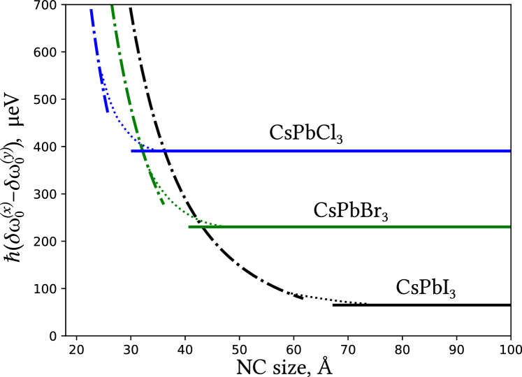
Figure 3: Bright exciton splitting due to NC anisotropy calculated in ${\bm{k}}\cdot{\bm{p}}$ approximation for three perovskite materials as a function of NC size assuming the 10% shape anisotropy of the NC. The ${\bm{k}}\cdot{\bm{p}}$ parameters are given in Table 1. Solid lines show the weak confinement regime (23), the dash-dotted lines the strong confinement regime (22) and the dashed lines are the guides to the eye.

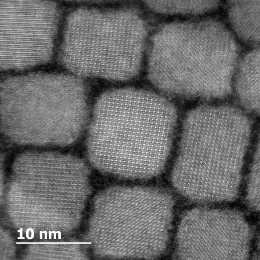
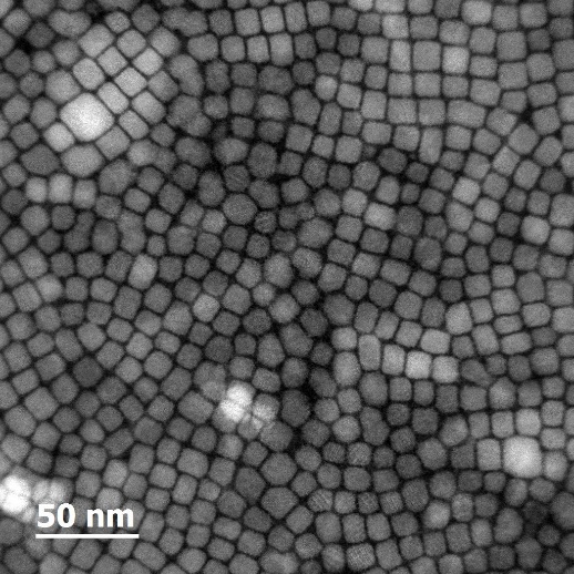
Figure 4: Atomic resolution ADF-STEM image of CsPbI₃ NCs studied here. The size of the NCs $\simeq$10 nm.

To estimate the value of $\delta_{\mathrm{an}}^{LR}$ we use the parameters of bulk perovskite CsPbI₃, CsPbBr₃, and CsPbCl₃. These parameters, taken from Ref. 5, are summarized in Table 1. The value of the interband momentum matrix element is estimated from the electron and hole masses assuming negligible contribution from the remote bands. From these parameters, using Eqs. (22,23), we calculated the value of the anisotropic splitting $\delta_{\mathrm{an}}^{LR}$ shown in Fig. 3 as a function of the NC size, for a fixed NC in-plane shape anisotropy of 10%. For CsPbI₃ NCs with the size of $\sim 10$ nm the anisotropic splitting due to the long-range electron-hole exchange interaction is approximately 65 $\mu$eV.

IV Synthesis of CsPbI₃ nanocrystals

Cesium lead iodide perovskite NCs (CsPbI₃ NCs) were synthesized following the method of Protesescu et al.Protesescu et al. (2015) First, Cs-oleate was prepared by mixing 0.814 g of Cs₂CO₃ with 40 mL of octadecene (ODE) and 2.5 mL of oleic acid (OA), with all reactants dried at 120^∘C for 1 h. The mixture was stirred at 150^∘C in an inert atmosphere until completion of the reaction. For the NCs formation, 5 mL of ODE and 0.188 mmol of lead (II) iodide (PbI₂) were dried for 1 h at 120^∘C in N₂ atmosphere. After the removal of moisture, 0.5 mL of dried OA and 0.5 mL of dried oleylamine were added to the reaction flask, and the temperature was raised up to 180^∘C. After complete solvation of the lead salt, 0.4 mL of the previously warmed up Cs-oleate solution was injected. A few seconds later, the NCs solution was quickly cooled down with an ice bath. The product was purified by centrifugation and subsequently redispersed in hexane. The synthesized colloidal solution was drop-cast deposited on a quartz glass substrate and dried until a continuous thin film was formed.

The sample was investigated by a JEOL 2100F scanning transmission electron microscope (STEM) equipped with a delta corrector, which compensates for the aberration up to the fifth order. Figure 4 shows the annular dark-field (ADF) STEM image of the drop-cast deposited CsPbI₃ NC ensemble with atomic resolution, revealing its closely packed morphology. From Fig. 4 we conclude that the NCs have the shape of the cuboid with edge size close to 10 nm and the average aspect ratio about 10%. One of the main axis of all NCs is normal to the layer plane and the orientation of the main axes of different NCs in the layer plane is random, so the layer as a whole is isotropic in the lateral direction. This fact is reflected in the spectroscopic measurements, see below.

V PL measurements

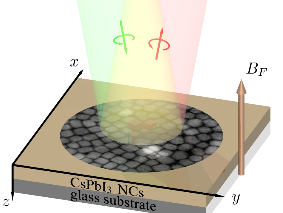
Figure 5: The geometry of the experiment.

The geometry of the experiment for studying polarized PL at cryogenic temperatures is shown in Fig. 5. PL was excited by a titanium-sapphire laser, tunable in the range of 700–820 nm in continuos wave regime. The beam of the excitation light was directed along the normal to the crystal surface ($z$-axis). The light spot diameter was $\simeq$150 $\mu$m, which is at least four orders of magnitude larger than typical NC size and guarantees averaging of the observed PL over the large number of NCs. The PL was detected in the backscattering geometry at a small angle to the $z$-axis, and recorded by the Horiba iHR-550 spectrometer and an avalanche photodiode (APD). The APD was connected to a scheme of the two-channel photon counting detector from which data was transferred to a computer. The sample was subjected to a longitudinal magnetic field $\textbf{B}_{F}\parallel z$ (Faraday geometry) produced by a resistive magnet. We note that the PL intensity considerably rises with the decrease of temperature from room temperature to the helium temperatures, contrary to e.g. Si NCs.Heitmann et al. (2004)

The experimental technique follows the work by Dzhioev et al. Dzhioev et al. (1997a). Polarized luminescence is determined completely by specifying four components of the Stokes parameters Blum (1981), which give the following information: (a) full light intensity $I$; (b) the degree of circular polarization; (c) the degree of linear polarization with respect to the pair of orthogonal axes ($x$, $y$); (d) the degree of linear polarization with respect to the axes ($x^{\prime}$, $y^{\prime}$) rotated by an angle of $45^{\circ}$ relative to the ($x$, $y$) axes around the $z$-axis.

We are interested only in the Stokes parameters related to the polarization of light. It should be borne in mind that in addition to the three Stokes parameters characterizing the polarization of the secondary radiation, it is also necessary to have full information on the polarization of the excitation light, which, in turn, is also characterized by three Stokes components. Thus, in the general case, we have a set of $3\times 3=9$ different measurements, because for each of the three polarizations of the excitation light it is possible to measure three Stokes parameters of the secondary radiation:

$$\rho_{c}^{\alpha}=\frac{I_{\sigma^{+}}^{\alpha}-I_{\sigma^{-}}^{\alpha}}{I_{\sigma^{+}}^{\alpha}+I_{\sigma^{-}}^{\alpha}},\;\rho_{\ell}^{\alpha}=\frac{I_{x}^{\alpha}-I_{y}^{\alpha}}{I_{x}^{\alpha}+I_{y}^{\alpha}},\;\rho_{\ell^{\prime}}^{\alpha}=\frac{I_{x^{\prime}}^{\alpha}-I_{y^{\prime}}^{\alpha}}{I_{x^{\prime}}^{\alpha}+I_{y^{\prime}}^{\alpha}},\;$$ (24)

where the upper index $\alpha$ indicates the polarization of the excitation light, which is set by a fixed polarizer in the excitation channel for right-handed circular polarization ($\alpha=\sigma^{+}$), linear polarization along $x$ ($\alpha=L$) and $x^{\prime}$ ($\alpha=L^{\prime}$) axes. Lower index refers to the registration channel, in which the analyzer modulates the circular polarization from $\sigma^{+}$ to $\sigma^{-}$ ($\rho_{c}^{\alpha}$), the linear polarization from the $x$- to the $y$-axis ($\rho_{\ell}^{\alpha}$), or the linear polarization from the $x^{\prime}$- to the $y^{\prime}$-axis ($\rho_{\ell^{\prime}}^{\alpha}$). The total PL intensity does not depend on the choice of the orthogonal components: $I=I_{\sigma^{+}}^{\alpha}+I_{\sigma^{-}}^{\alpha}=I_{x}^{\alpha}+I_{y}^{\alpha}=I_{x^{\prime}}^{\alpha}+I_{y^{\prime}}^{\alpha}$.

However, instead of measuring the polarization degrees $\rho_{c}^{\alpha}$, $\rho_{\ell}^{\alpha}$ and $\rho_{\ell^{\prime}}^{\alpha}$ defined in accordance with (24), we applied a modulation technique where the analyzer is in a fixed position and the sample is pumped by the incident light changing its polarization from a circular or linear to the orthogonal at a frequency of 42 kHz. In this case, the setup measures the effective Stokes parameters

$$\rho^{c}_{\alpha}=\frac{I^{\sigma^{+}}_{\alpha}-I^{\sigma^{-}}_{\alpha}}{I^{\sigma^{+}}_{\alpha}+I^{\sigma^{-}}_{\alpha}},\;\rho^{\ell}_{\alpha}=\frac{I^{x}_{\alpha}-I^{y}_{\alpha}}{I^{x}_{\alpha}+I^{y}_{\alpha}},\;\rho^{\ell^{\prime}}_{\alpha}=\frac{I^{x^{\prime}}_{\alpha}-I^{y^{\prime}}_{\alpha}}{I^{x^{\prime}}_{\alpha}+I^{y^{\prime}}_{\alpha}},\;$$ (25)

where the lower index fixes the position of the analyzer and the top index refers to the excitation channel, whose polarization is modulated. This technique allows one to avoid the effects of dynamic nuclear polarization. Strictly speaking, the polarization parameters, defined by the formulas (24) and (25), are different. However, it is possible to show Dzhioev et al. (1997b) that if the effects of dichroism (circular or linear) are negligible, then equations (25) can be considered as the usual Stokes parameters, which characterize circularly (or linearly) polarized luminescence in the case of polarized excitation.

An appearance of the circularly polarized excitonic PL under the circularly polarized excitation ($\rho^{c}_{\sigma^{+}}\not=0$) is known as the optical orientation of excitons,Bir and Pikus (1972); Pikus and Ivchenko (1982) while the linear polarization of the excitonic PL under the linearly polarized excitation ($\rho_{L}^{\ell},\rho_{L^{\prime}}^{\ell^{\prime}}\not=0$) is known as the optical alignment of excitons. An appearance of the circular (linear) polarization of the PL under the linear (circular) excitation is referred to as conversion of the orientation to alignment (alignment to orientation).

VI Experimental results

Figure 6a shows the spectral dependencies of PL intensity, $I(\lambda)$, and PL optical orientation, $\rho^{c}_{\sigma^{+}}(\lambda)$, in zero magnetic field at the excitation wavelength $\lambda_{\mathrm{ex}}=705$ nm, power density $W=0.6$ W/cm², and temperature $T=2$ K. Polarization measurements in a longitudinal magnetic field were carried out at $\lambda_{\mathrm{det}}=721$ nm, which corresponds to the maximum of the PL intensity. An external magnetic field, $B_{F}$, restores the optical orientation (increases the degree of circular polarization), see Fig. 6b. An optical alignment of $\rho_{L}^{\ell}=13$% is observed in PL when exciting with light linearly polarized along the $x$-axis in zero field, see Fig. 6c. The observed optical alignment is virtually isotropic: when illuminated by light polarized along the $x^{\prime}$, the polarization degree is $\rho_{L^{\prime}}^{\ell^{\prime}}=14$%, see Fig. 6d. This indicates a random distribution of dipoles over the ensemble of NCs. The degree of linear polarization decreases with increasing magnetic field. This indicates that the phenomena of optical orientation and alignment in this system have the same physical nature.

The suppression of the optical orientation at zero magnetic field, together with the strong optical alignment of excitons indicates that the bright exciton state is split at zero field into linearly polarized components. It is worth to note that there is a non-zero polarization $\rho^{c}_{\sigma^{+}}=4$% at zero magnetic field. In a transverse magnetic field polarization decreases in a characteristic field of 7 mT. This contribution may originate from the excitons in cubic phase NCs, single electrons, or trions. This will be considered in more details in another work, but the small residual circular polarization and strong optical alignment indicate that, in our experiments, the trions which are known to dominate the optical properties of similar systemsCanneson et al. (2017) do not affect our results significantly.

Note that the transformation (conversion) of one polarization of excitons into another (for example, the appearance of linear polarization under circularly polarized pumping) is absent. Alignment of excitons is the hallmark of the anisotropy of the system, either microscopical or mesoscopical. The absence of polarization conversion shows that there are almost no NCs with degenerate bright exciton states.

The optical orientation experiments reveal the structure of exciton levels and allow one to measure the magnitude of the splitting of the exciton bright state, $\delta_{\mathrm{an}}$, averaged over an ensemble of NCs, even in the absence of a sufficient spectral resolution. In a weak magnetic field ($B_{F}\ll\delta_{\mathrm{an}}/\mu_{B}g_{X}\equiv b$, where $g_{X}$ is the exciton $g$-factor, $\mu_{B}$ is the Bohr magneton) the circular polarization of PL is absent because the $\sigma^{\pm}$-light excites a coherent superposition of the $x$- and $y$-states split by $\delta_{\mathrm{an}}\simeq 120$ $\mu$eV. This splitting causes fast beats between the two eigenstates which average circular polarization out during the exciton lifetime $\tau\sim 0.2$ ns ($\tau\gg\hbar/\delta_{\mathrm{an}}\sim 10$ ps).Fu et al. (2017) When the magnetic field increases ($B_{F}\geq b$), the degree of the PL circular polarization also increases, thus restoring optical orientation of the excitons. The optical orientation is completely restored when $B_{F}\gg b$. In turn, the optical alignment of the excitons already exists in zero magnetic field when excitation light is polarized along the $x$ or $y$ axis. Magnetic field $B_{F}>b$ converts $\left|x/y\right\rangle$ states into $\left|\pm 1\right\rangle$ states decreasing the linear polarization of the PL, as illustrated in Fig. 2.

Here we do not explicitly consider the role of the dark exciton and the $z$-polarized states of the bright excitons. When the dark exciton states have energy close to the bright ones, one may observe the resonance in the PL polarization intensity due to the anticrossong between dark and bright excitons.Ivchenko and Kaminskii (1995); Gourdon et al. (1998) In our experiments, this anticrossing is not present and we conclude that the possible presence of the dark excitons does not affect the polarized PL signal. The presence of $z$-polarized bright excitons may not affect the circular polarization profile, though it may in principle affect its amplitude. The $z$-polarized bright exciton state may contribute to the linear polarization $\rho^{\ell}_{L}(B_{F})$, $\rho^{\ell^{\prime}}_{L^{\prime}}(B_{F})$. However, as long as all three polarizations in Fig.  6 b,c,d are perfectly fitted using the same set of parameters, we conclude that in our experiments $z$-polarized bright excitons do not contribute to the linear polarization as well.

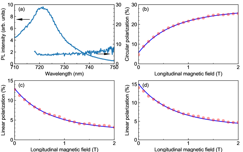
Figure 6: Polarization spectroscopy of the PL of the sample at $\lambda_{\mathrm{ex}}=705$ nm, $W=0.6$ W/cm², $T=2$ K. (a) PL spectra and optical orientation at zero magnetic field. Symbols show the polarization measurements of the PL in the longitudinal field detected at $\lambda_{\mathrm{det}}=721$ nm: (b) optical orientation $\rho^{c}_{\sigma^{+}}(B_{F})$; optical alignment $\rho_{L}^{\ell}(B_{F})$ (c) and (d) $\rho_{L^{\prime}}^{\ell^{\prime}}(B_{F})$. In panels b,c,d the fit of the polarization after Eqs. (28), (29) averaged over shape anisotropy distribution (27) is shown in solid lines, see text.

In order to describe the PL polarization measurements, one can introduce the exchange-related frequencies $\Omega_{x}$ and $\Omega_{y}$ as the coefficients in the effective Hamiltonian for the radiative doublet $\left|\pm 1\right\rangle$Dzhioev et al. (1997a)

$$\mathcal{H}_{\mathrm{eff}}=\frac{1}{2}\begin{pmatrix}\mu_{B}g_{X}B_{F}&\hbar\Omega_{x}-i\hbar\Omega_{y}\\ \hbar\Omega_{x}+i\hbar\Omega_{y}&-\mu_{B}g_{X}B_{F}\end{pmatrix}\,.$$ (26)

In the following we neglect the exciton spin relaxation.

To average over the ensemble, one has to assume the distribution function of the exchange splitting $\delta_{\mathrm{an}}$. When the short-range exchange contribution to the splitting is small compared with the long-range exchange one, the splitting is proportional to the shape anisotropy, see Eq. (20, 21). The distribution of the shape anisotropy is typically Gaussian:Elazzouzi-Hafraoui et al. (2008)

$$\mathcal{P}(\Omega)=\frac{1}{\sigma_{\delta}\sqrt{2\pi}}\exp\left[-\frac{\Omega^{2}}{2\sigma_{\delta}^{2}}\right]\;,$$ (27)

where $\sigma_{\delta}$ is the dispersion of the long range exchange splitting and the amplitude of the splitting for given NC is $\Omega$. Note that the orientation of the NC principal axes in the layer is random, which results in i.e., $\langle\Omega_{x}\Omega_{y}\rangle=0$

The averaging over the lateral distribution of the orientation of NCs is easier to consider separately: assuming the NCs with splitting of linearly polarized states $\Omega$ with the random distribution of principal axes in the substrate plane and assuming the exciton lifetime in the radiative states $\left|\pm 1\right\rangle$, $\tau\gg 1/\Omega$, one can obtain for the PL circular polarization under resonant circularly-polarized excitation in the longitudinal magnetic fieldDzhioev et al. (1997a); Ivchenko (2005)

$$P_{c}(B_{z};\Omega)=P_{c}(0)\frac{\left(\mu_{B}g_{X}B_{F}\right)^{2}}{\left(\mu_{B}g_{X}B_{F}\right)^{2}+\hbar^{2}\Omega^{2}}\>.$$ (28)

Similar consideration gives for the linear polarizationDzhioev et al. (1997a); Ivchenko (2005)

$$P_{\ell}(B_{z};\Omega)=P_{\ell}(0)\frac{\hbar^{2}\Omega^{2}}{\left(\mu_{B}g_{X}B_{F}\right)^{2}+\hbar^{2}\Omega^{2}}\>.$$ (29)

The polarization for the ensemble of different NCs is then obtained by averaging of Eqs. (28, 29) over the distribution of the exciton splitting (27):

$$P_{\xi}(B_{z})=\int\mathcal{P}(\Omega)P_{\xi}(B_{z};\Omega)d\Omega$$ (30)

In Fig. 6 b,c,d we show the results of the fit of the optical orientation and alignment experimental measurements using Eqs. (27-30) assuming the long-range exchange origin of the splitting caused by the NC shape (27) (solid line). In fitting procedure we assume that there is additional polarization caused by other mechanisms: presence of trions for circular polarization and dichroism for the linear polarization. Both the amplitude of the polarization $P_{\xi}(0)$ and the shifts $\Delta P_{\xi}$ are considered as free parameters. From the best fit we extract the dispersion of the long-range exchange splitting $\sigma_{\delta}$.

The best fit assuming Gaussian distribution of the bright exciton splittings (27) gives an excellent agreement with experimental data for $\hbar\sigma_{\delta}/\mu_{B}g_{X}=0.917$ T. Using the exciton $g$-factor extracted from Raman data $g_{X}\simeq 2.3$ (which is close to typical value in similar systems, see Ref. Fu et al., 2017) we may extract the value of the dispersion of the long-range exchange splitting $\hbar\sigma_{\delta}=122$ $\mu$eV. In experiment, we have the Gaussian distribution of NC shape anisotropy with the standard deviation 10%, see Fig. 4. This means that the optical orientation may be explained if we assume that for 10% shape anisotropy we have the bright exciton splitting 122 $\mu$eV and this splitting is proportional to the shape anisotropy.

There is also a possibility to explain the optical orientation and alignment assuming that the splitting of the bright excitons originates from the short-range exchange splitting $\delta_{\mathrm{an}}^{SR}$ and the long-range exchange is negligible. The NCs are located on the substrate randomly, with one of the principal axes of each NC normal to the substrate plane, which means that for each NC the splitting is equally distributed between three possibilities: $\delta_{1}^{SR}$, $\delta_{2}^{SR}$, or $\delta_{1}^{SR}-\delta_{2}^{SR}$. The results of polarization spectroscopy in Fig. 6 may also be quite well fitted under this assumption with the crystal-field splittings of bright excitons $\delta_{1}^{SR}=123$ $\mu$eV and $\delta_{2}^{SR}=14$ $\mu$eV.

VII Discussion

The value of the bright exciton fine structure splitting, averaged over an ensemble of CsPbI₃ NCs, measured in our experiment is close to $120$ $\mu$eV. This value exceeds our theoretical estimate of $65$ $\mu$eV for the bright exciton splitting resulting from the NC shape anisotropy of 10 % and caused by the long-range electron-hole exchange interaction. However, it is $1.5$ to $5$ times less than the values measured on individual NCs in Ref. 15, although the mean size of the NCs was about the same. Moreover, Yin et al. emphasized that they also investigated some samples, where the fine structure splittings for all NCs, on which they performed single-dot measurements, were below their spectral resolution of $200$ $\mu$eV, although the same synthesis procedure was nominally adopted for all the samples.Yin et al. (2017) Provided that the cesium lead halide perovskites are known to feature different crystal phases and that co-existence of these phases in nanostructures has been reported,Yu et al. (2016) one can speculate that, under some conditions, which are difficult to control, the NCs can have different phases or be inhomogeneous, which would affect their exciton fine-structure splittings.

Indeed, in addition to the long-range electron-hole exchange interaction, which is sensitive to the NC shape anisotropy, there is its short-range counterpart sensitive to the underlying crystal phase. In the cubic phase, the anisotropic part of the short-range (analytic) electron-hole exchange interaction is zero. In the tetragonal phase, the additional anisotropy of the short-range (analytic) electron-hole exchange interaction does not necessarily affect the splitting between the $x$- and $y$-polarized exciton states ($\delta_{2}^{SR}=0$), while our estimates show that the long-range (non-analytic) exchange interaction is comparable with the observed anisotropic splitting. In the orthorhombic phase, however, the long-range (non-analytic) electron-hole exchange interaction has an additional in-plane anisotropy, and there may be a significant contribution from the short-range electron-hole exchange interaction to the anisotropic splitting.

Note that, if we assume tetragonal phase of the NCs, then taking into account only the short-range part of the exchange interaction cannot explain our results. The polarization dependencies of Fig. 6 cannot be fitted if one takes $\delta_{2}^{SR}=0$.

VIII Conclusion

In conclusion, we have presented measurements of optical orientation and alignment of excitons in ensembles of CsPbI₃ NCs at cryogenic temperatures. From our experiment we conclude that there is an anisotropic splitting of bright exciton levels in NCs. The experimental data may be fitted if one assumes that the splitting is related to the NC shape anisotropy and amounts 122 $\mu$eV. Our theoretical estimate, basing on the not-well-known value of the interband momentum matrix element for CsPbI₃ and assuming 10% NC shape anisotropy, extracted from the TEM measurements, gives about half of this value. We note, however, that both the anisotropic shape of NCs and the possible low-symmetry phase of the underlying crystal structure, as well as a combination thereof, may cause the anisotropic fine-structure splitting; optical spectroscopy alone cannot be used to rule out either of these possibilities. Further investigations are called for to unambiguously determine the crystal phase of cesium lead halide NCs at cryogenic temperatures and to determine the value of the interband momentum matrix element for CsPbX₃ (X=I, Br, Cl).

References

- Green et al. (2014) M. A. Green, A. Ho-Baillie, and H. J. Snaith, Nat Photon 8, 506 (2014).
- (2) T. C. Sum and N. Mathews, Energy Environ. Sci. 7, 2518.
- Zhang et al. (2015) C. Zhang, D. Sun, C.-X. Sheng, Y. X. Zhai, K. Mielczarek, A. Zakhidov, and Z. V. Vardeny, Nat Phys 11, 427 (2015), article.
- Odenthal et al. (2017) P. Odenthal, W. Talmadge, N. Gundlach, R. Wang, C. Zhang, D. Sun, Z.-G. Yu, Z. Valy Vardeny, and Y. S. Li, Nat Phys advance online publication, 4145 (2017).
- Protesescu et al. (2015) L. Protesescu, S. Yakunin, M. I. Bodnarchuk, F. Krieg, R. Caputo, C. H. Hendon, R. X. Yang, A. Walsh, and M. V. Kovalenko, Nano Letters 15, 3692 (2015).
- Tan et al. (2014) Z.-K. Tan, R. S. Moghaddam, M. L. Lai, P. Docampo, R. Higler, F. Deschler, M. Price, A. Sadhanala, L. M. Pazos, D. Credgington, F. Hanusch, T. Bein, H. J. Snaith, and R. H. Friend, Nat Nano 9, 687 (2014), letter.
- Xing et al. (2014) G. Xing, N. Mathews, S. S. Lim, N. Yantara, X. Liu, D. Sabba, M. Grätzel, S. Mhaisalkar, and T. C. Sum, Nat Mater 13, 476 (2014), letter.
- Yakunin et al. (2015) S. Yakunin, L. Protesescu, F. Krieg, M. I. Bodnarchuk, G. Nedelcu, M. Humer, G. D. Luca, M. Fiebig, W. Heiss, and M. V. Kovalenko, Nature Communications 6, 8056 (2015).
- Makarov et al. (2016) N. S. Makarov, S. Guo, O. Isaienko, W. Liu, I. Robel, and V. I. Klimov, Nano Letters 16, 2349 (2016).
- Lin et al. (2016) J. Lin, L. Gomez, C. de Weerd, Y. Fujiwara, K. Suenaga, and T. Gregorkiewicz, Nano Lett. 16, 7198 (2016).
- de Weerd et al. (2016) C. de Weerd, L. Gomez, H. Zhang, W. J. Buma, G. Nedelcu, M. V. Kovalenko, and T. Gregorkiewicz, J. Phys. Chem. C 120, 13310 (2016).
- de Jong et al. (2017) E. M. L. D. de Jong, G. Yamashita, L. Gomez, M. Ashida, Y. Fujiwara, and T. Gregorkiewicz, J. Phys. Chem. C 121, 1941 (2017).
- Becker et al. (2018) M. A. Becker, R. Vaxenburg, G. Nedelcu, P. C. Serce, A. Shabaev, M. J. Mehl, J. G. Michopoulos, S. G. Lambrakos, N. Bernstein, J. L. Lyons, T. Stöferle, R. F. Mahrt, M. V. Kovalenko, D. J. Norris, G. Rainò, and A. L. Efros, Nature 553, 189 (2018).
- Fu et al. (2017) M. Fu, P. Tamarat, H. Huang, J. Even, A. L. Rogach, and B. Lounis, Nano Letters 17, 2895 (2017).
- Yin et al. (2017) C. Yin, L. Chen, N. Song, Y. Lv, F. Hu, C. Sun, W. W. Yu, C. Zhang, X. Wang, Y. Zhang, and M. Xiao, Phys. Rev. Lett. 119, 026401 (2017).
- Canneson et al. (2017) D. Canneson, E. V. Shornikova, D. R. Yakovlev, T. Rogge, A. A. Mitioglu, M. V. Ballottin, P. C. M. Christianen, E. Lhuillier, M. Bayer, and L. Biadala, Nano Letters (2017), 10.1021/acs.nanolett.7b02827, article ASAP.
- Pikus and Ivchenko (1982) G. E. Pikus and E. L. Ivchenko, Excitons, edited by E. I. Rashba and M. D. Struge (North-Holland, Amsterdam, 1982) p. 205.
- Planel and Benoit a la Guillaume (1984) R. Planel and C. Benoit a la Guillaume, in Optical orientation, edited by F. Meier and B. P. Zakharchenya (North-Holland, Amsterdam, 1984) p. 353.
- Ivchenko (1995) E. L. Ivchenko, Pure Appl. Chem. 67, 463 (1995).
- Ivchenko and Pikus (2095) E. L. Ivchenko and G. E. Pikus, Superlattices and other heterostructures. Symmetry and Optical Phenomena (Springer-Verlag, Berlin, 2095).
- Dzhioev et al. (1997a) R. I. Dzhioev, B. P. Zakharchenya, E. L. Ivchenko, V. L. Korenev, Y. G. Kusraev, N. N. Ledentsov, V. M. Ustinov, A. E. Zhukov, and A. F. Tsatsul’nikov, JETP Lett. 65, 804 (1997a), [Pis’ma Zh. Eksp. Teor. Fiz 65, 766 (1997)].
- Dzhioev et al. (1997b) R. I. Dzhioev, H. M. Gibbs, E. L. Ivchenko, G. Khitrova, V. L. Korenev, M. N. Tkachuk, and B. P. Zakharchenya, Phys. Rev. B 56, 13405 (1997b).
- Dzhioev et al. (1998a) R. I. Dzhioev, B. P. Zakharchenya, V. L. Korenev, P. E. Pak, D. A. Vinokurov, O. V. Kovalenkov, and I. S. Tarasov, Physics of the Solid State 40, 1587 (1998a), [Fiz. Tv. Tela 40 (9), 1745 (1998)].
- Dzhioev et al. (1998b) R. I. Dzhioev, B. P. Zakharchenya, E. L. Ivchenko, V. L. Korenev, Y. G. Kusraev, N. N. Ledentsov, V. M. Ustinov, A. E. Zhukov, and A. F. Tsatsul’nikov, Physics of the Solid State 40, 790 (1998b), [Fiz. Tv. Tela 40(5), 858 (1998)].
- Dzhioev et al. (2003) R. Dzhioev, V. Korenev, M. Lazarev, V. Sapega, R. Notzel, and K. Ploog, in Optical properties of 2D systems with interacting electrons, edited by W. J. Ossau and R. Suris (Kluwer Academic Publishers, 2003) p. 233.
- Møller (1958) C. K. Møller, Nature 182, 1436 (1958).
- Fujii et al. (1974) Y. Fujii, S. Hoshino, Y. Yamada, and G. Shirane, Phys. Rev. B 9, 4549 (1974).
- Yu et al. (2016) Y. Yu, D. Zhang, C. Kisielowski, L. Dou, N. Kornienko, Y. Bekenstein, A. B. Wong, A. P. Alivisatos, and P. Yang, Nano Letters 16, 7530 (2016).
- Haruyama et al. (2016) J. Haruyama, K. Sodeyama, L. Han, and Y. Tateyama, Accounts of Chemical Research 49, 554 (2016).
- Murali et al. (2016) B. Murali, S. Dey, A. L. Abdelhady, W. Peng, E. Alarousu, A. R. Kirmani, N. Cho, S. P. Sarmah, M. R. Parida, M. I. Saidaminov, A. A. Zhumekenov, J. Sun, M. S. Alias, E. Yengel, B. S. Ooi, A. Amassian, O. M. Bakr, and O. F. Mohammed, ACS Energy Letters 1, 1119 (2016).
- Wang et al. (2017) C. Wang, A. S. R. Chesman, and J. J. Jasieniak, Chem. Commun. 53, 232 (2017).
- Cottingham and Brutchey (2016) P. Cottingham and R. L. Brutchey, Chem. Commun. 52, 5346 (2016).
- Even et al. (2015) J. Even, L. Pedesseau, C. Katan, M. Kepenekian, J.-S. Lauret, D. Sapori, and E. Deleporte, The Journal of Physical Chemistry C 119, 10161 (2015).
- Even (2015) J. Even, The Journal of Physical Chemistry Letters 6, 2238 (2015).
- Yu (2016) Z. G. Yu, Sci. Rep. 6, 28576 (2016).
- Ivchenko (2005) E. Ivchenko, Optical Spectroscopy of Semiconductor Nanostructures (Alpha Science, 2005).
- Bir and Pikus (1974) G. Bir and G. Pikus, Symmetry and Strain-Induced Effects in Semiconductors (Wiley, New York, 1974).
- Denisov and Makarov (1973) M. M. Denisov and V. P. Makarov, phys. stat. sol. (b) 56, 9 (1973).
- Goupalov et al. (1998a) S. V. Goupalov, E. L. Ivchenko, and A. V. Kavokin, JETP 86, 388 (1998a), [Zh. Eksp. Teor. Fiz. 113, 703 (1998)].
- Goupalov et al. (1998b) S. V. Goupalov, E. L. Ivchenko, and A. V. Kavokin, Superlatt. Microstruct. 23, 1205 (1998b).
- Dvorak et al. (2013) M. Dvorak, S.-H. Wei, and Z. Wu, Phys. Rev. Lett. 110, 016402 (2013).
- Pikus and Bir (1971) G. Pikus and G. Bir, JETP 33, 108 (1971), [Zh. Eksp. Teor. Fiz.60, 195 (1971)].
- Goupalov and Ivchenko (1998) S. V. Goupalov and E. L. Ivchenko, J. Crystal Growth 184/185, 393 (1998).
- Goupalov and Ivchenko (2000) S. V. Goupalov and E. L. Ivchenko, Phys. Sol. State 42, 2030 (2000), [Fiz. Tverd. Tela, 42, 1976 (2000)].
- Goupalov and Ivchenko (2001) S. V. Goupalov and E. L. Ivchenko, Phys. Sol. State 43, 1867 (2001), [Fiz. Tverd. Tela 43, 1791 (2001)].
- Goupalov et al. (2003) S. V. Goupalov, P. Lavallard, G. Lamouche, and D. S. Citrin, Phys. Sol. State 45, 768 (2003), [Fiz. Tverd. Tela 45, 730 (2003)].
- Heitmann et al. (2004) J. Heitmann, F. Müller, L. Yi, M. Zacharias, D. Kovalev, and F. Eichhorn, Phys. Rev. B 69, 195309 (2004).
- Blum (1981) K. Blum, Density Matrix Theory and Applications, 1st ed. (Plenum Press, New York and London, 1981).
- Bir and Pikus (1972) G. L. Bir and G. E. Pikus, JETP Lett. 15, 516 (1972), [Pis’ma Zh. Eksp. Teeor. Fiz 15, 730 (1972)].
- Ivchenko and Kaminskii (1995) E. L. Ivchenko and A. Y. Kaminskii, Fiz. Tverd. Tela 37, 1418 (1995), [Sov. Phys. Solid State 37, 768 (1995)].
- Gourdon et al. (1998) C. Gourdon, I. V. Mashkov, P. Lavallard, and R. Planel, Phys. Rev. B 57, 3955 (1998).
- Elazzouzi-Hafraoui et al. (2008) S. Elazzouzi-Hafraoui, Y. Nishiyama, J.-L. Putaux, L. Heux, F. Dubreuil, and C. Rochas, Biomacromolecules 9, 57 (2008).
- Note (1) We give only one linear polarizaion because in the isotropic system .
- Note (2) For completeness, the fit in Fig. 6b,c,d is given for the following values: , , , , , .
- Note (3) V.F. Sapega, unpublished.