An Instability in Variational Inference for Topic Models

Abstract

Topic models are Bayesian models that are frequently used to capture the latent structure of certain corpora of documents or images. Each data element in such a corpus (for instance each item in a collection of scientific articles) is regarded as a convex combination of a small number of vectors corresponding to ‘topics’ or ‘components’. The weights are assumed to have a Dirichlet prior distribution. The standard approach towards approximating the posterior is to use variational inference algorithms, and in particular a mean field approximation.

We show that this approach suffers from an instability that can produce misleading conclusions. Namely, for certain regimes of the model parameters, variational inference outputs a non-trivial decomposition into topics. However –for the same parameter values– the data contain no actual information about the true decomposition, and hence the output of the algorithm is uncorrelated with the true topic decomposition. Among other consequences, the estimated posterior mean is significantly wrong, and estimated Bayesian credible regions do not achieve the nominal coverage. We discuss how this instability is remedied by more accurate mean field approximations.

1 Introduction

Topic modeling [Ble12] aims at extracting the latent structure from a corpus of documents (either images or texts), that are represented as vectors ${\boldsymbol{x}}_{1},{\boldsymbol{x}}_{2},\dots,{\boldsymbol{x}}_{n}\in\mathbb{R}^{d}$. The key assumption is that the $n$ documents are (approximately) convex combinations of a small number $k$ of topics $\tilde{\boldsymbol{h}}_{1},\dots,\tilde{\boldsymbol{h}}_{k}\in\mathbb{R}^{d}$. Conditional on the topics, documents are generated independently by letting

$${\boldsymbol{x}}_{a}=\frac{\sqrt{\beta}}{d}\sum_{\ell=1}^{k}w_{a,\ell}\tilde{\boldsymbol{h}}_{\ell}+{\boldsymbol{z}}_{a}\,,$$ (1.1)

where the weights ${\boldsymbol{w}}_{a}=(w_{a,\ell})_{1\leq\ell\leq k}$ and noise vectors ${\boldsymbol{z}}_{a}$ are i.i.d. across $a\in\{1,\dots,n\}$. The scaling factor $\sqrt{\beta}/d$ is introduced for mathematical convenience (an equivalent parametrization would have been to scale ${\boldsymbol{Z}}$ by a noise-level parameter $\sigma$), and $\beta>0$ can be interpreted as a signal-to-noise ratio. It is also useful to introduce the matrix $\boldsymbol{X}\in\mathbb{R}^{n\times d}$ whose $i$-th row is ${\boldsymbol{x}}_{i}$, and therefore

$$\boldsymbol{X}=\frac{\sqrt{\beta}}{d}\,{\boldsymbol{W}}{\boldsymbol{H}}^{{\sf T}}+{\boldsymbol{Z}}\,,$$ (1.2)

where ${\boldsymbol{W}}\in\mathbb{R}^{n\times k}$ and ${\boldsymbol{H}}\in\mathbb{R}^{d\times k}$. The $a$-th row of ${\boldsymbol{W}}$, is the vector of weights ${\boldsymbol{w}}_{a}$, while the rows of ${\boldsymbol{H}}$ will be denoted by ${\boldsymbol{h}}_{i}\in\mathbb{R}^{k}$.

Note that ${\boldsymbol{w}}_{a}$ belongs to the simplex ${\sf P}_{1}(k)=\{{\boldsymbol{w}}\in\mathbb{R}^{k}_{\geq 0}\;:\;\;\langle{\boldsymbol{w}},{\boldsymbol{1}}_{k}\rangle=1\}$. It is common to assume that its prior is Dirichlet: this class of models is known as Latent Dirichlet Allocations, or LDA [BNJ03]. Here we will take a particularly simple example of this type, and assume that the prior is Dirichlet in $k$ dimensions with all parameters equal to $\nu$ (which we will denote by ${\rm Dir}(\nu;k)$). As for the topics ${\boldsymbol{H}}$, their prior distribution depends on the specific application. For instance, when applied to text corpora, the $\tilde{\boldsymbol{h}}_{i}$ are typically non-negative and represent normalized word count vectors. Here we will make the simplifying assumption that they are standard Gaussian $(\tilde{\boldsymbol{h}}_{i})_{i\leq d}\sim_{iid}{\sf N}(0,{\boldsymbol{I}}_{k})$. Finally, ${\boldsymbol{Z}}$ will be a noise matrix with entries $(Z_{ij})_{i\in[n],j\in[d]}\sim_{iid}{\sf N}(0,1/d)$.

In fully Bayesian topic models, the parameters of the Dirichlet distribution, as well as the topic distributions are themselves unknown and to be learned from data. Here we will work in an idealized setting in which they are known. We will also assume that data are in fact distributed according to the postulated generative model. Since we are interested in studying some limitations of current approaches, our main point is only reinforced by assuming this idealized scenario.

As is common with Bayesian approaches, computing the posterior distribution of the factors ${\boldsymbol{H}}$, ${\boldsymbol{W}}$ given the data $\boldsymbol{X}$ is computationally challenging. Since the seminal work of Blei, Ng and Jordan [BNJ03], variational inference is the method of choice for addressing this problem within topic models. The term ‘variational inference’ refers to a broad class of methods that aim at approximating the posterior computation by solving an optimization problem, see [JGJS99, WJ08, BKM17] for background. A popular starting point is the Gibbs variational principle, namely the fact that the posterior solves the following convex optimization problem:

$$p_{{\boldsymbol{W}},{\boldsymbol{H}}|\boldsymbol{X}}(\,\cdot\,,\cdot,|\boldsymbol{X}) =\arg\min_{q\in{\mathcal{P}}_{n,d,k}}{\rm KL}(q\|p_{{\boldsymbol{W}},{\boldsymbol{H}}|\boldsymbol{X}})$$ (1.3)

$$=\arg\min_{q\in{\mathcal{P}}_{n,d,k}}\Big{\{}-{\mathbb{E}}_{q}\log p_{\boldsymbol{X}|{\boldsymbol{W}},{\boldsymbol{H}}}(\boldsymbol{X}|{\boldsymbol{H}},{\boldsymbol{W}})+{\rm KL}(q\|p_{{\boldsymbol{W}}}\times p_{{\boldsymbol{H}}})\Big{\}}\,,$$ (1.4)

where ${\rm KL}(\,\cdot\,\|\,\cdot\,)$ denotes the Kullback-Leibler divergence. The variational expression in Eq. (1.4) is also known as the Gibbs free energy. Optimization is within the space ${\mathcal{P}}_{n,d,k}$ of probability measures on ${\boldsymbol{H}},{\boldsymbol{W}}$. To be precise, we always assume that a dominating measure $\nu_{0}$ over $\mathbb{R}^{n\times k}\times\mathbb{R}^{d\times k}$ is given for ${\boldsymbol{W}},{\boldsymbol{H}}$, and both $p_{{\boldsymbol{W}},{\boldsymbol{H}}|\boldsymbol{X}}$ and $q$ have densities with respect to $\nu_{0}$: we hence identify the measure with its density. Throughout the paper (with the exception of the example in Section 2) $\nu_{0}$ can be taken to be the Lebesgue measure.

Even for ${\boldsymbol{W}},{\boldsymbol{H}}$ discrete, the Gibbs principle has exponentially many decision variables. Variational methods differ in the way the problem (1.3) is approximated. The main approach within topic modeling is naive mean field, which restricts the optimization problem to the space of probability measures that factorize over the rows of ${\boldsymbol{W}},{\boldsymbol{H}}$:

$$\hat{q}\left({\boldsymbol{W}},{\boldsymbol{H}}\right)=q\left({\boldsymbol{H}}\right)\tilde{q}\left({\boldsymbol{W}}\right)=\prod_{i=1}^{d}q_{i}\left({\boldsymbol{h}}_{i}\right)\prod_{a=1}^{n}\tilde{q}_{a}\left({\boldsymbol{w}}_{a}\right)\,.$$ (1.5)

By a suitable parametrization of the marginals $q_{i}$, $\tilde{q}_{a}$, this leads to an optimization problem of dimension $O((n+d)k)$, cf. Section 3. Despite being non-convex, this problem is separately convex in the $(q_{i})_{i\leq d}$ and $(\tilde{q}_{a})_{a\leq n}$, which naturally suggests the use of an alternating minimization algorithm which has been successfully deployed in a broad range of applications ranging from computer vision to genetics [FFP05, WB11, RSP14]. We will refer to this as to the naive mean field iteration. Following a common use in the topics models literature, we will use the terms ‘variational inference’ and ‘naive mean field’ interchangeably.

The main result of this paper is that naive mean field presents an instability for learning Latent Dirichlet Allocations. We will focus on the limit $n,d\to\infty$ with $n/d=\delta$ fixed. Hence, an LDA distribution is determined by the parameters $(k,\delta,\nu,\beta)$. We will show that there are regions in this parameter space such that the following two findings hold simultaneously:

No non-trivial estimator.

Any estimator ${\widehat{\boldsymbol{H}}}$, $\widehat{\boldsymbol{W}}$ of the topic or weight matrices is asymptotically uncorrelated with the real model parameters ${\boldsymbol{H}},{\boldsymbol{W}}$. In other words, the data do not contain enough signal to perform any strong inference.

Variational inference is randomly biased.

Given the above, one would hope the Bayesian posterior to be centered on an unbiased estimate. In particular, $p({\boldsymbol{w}}_{a}|\boldsymbol{X})$ (the posterior distribution over weights of document $a$) should be centered around the uniform distribution ${\boldsymbol{w}}_{a}=(1/k,\dots,1/k)$. In contrast, we will show that the posterior produced by naive mean field is centered around a random distribution that is uncorrelated with the actual weights. Similarly, the posterior over topic vectors is centered around random vectors uncorrelated with the true topics.

One key argument in support of Bayesian methods is the hope that they provide a measure of uncertainty of the estimated variables. In view of this, the failure just described is particularly dangerous because it suggests some measure of certainty, although the estimates are essentially random.

Is there a way to eliminate this instability by using a better mean field approximation? We show that a promising approach is provided by a classical idea in statistical physics, the Thouless-Anderson-Palmer (TAP) free energy [TAP77, OW01]. This suggests a variational principle that is analogous in form to naive mean field, but provides a more accurate approximation of the Gibbs principle:

Variational inference via the TAP free energy.

We show that the instability of naive mean field is remedied by using the TAP free energy instead of the naive mean field free energy. The latter can be optimized using an iterative scheme that is analogous to the naive mean field iteration and is known as approximate message passing (AMP).

While the TAP approach is promising –at least for synthetic data– we believe that further work is needed to develop a reliable inference scheme.

The rest of the paper is organized as follows. Section 2 discusses a simpler example, ${\mathbb{Z}}_{2}$-synchronization, which shares important features with latent Dirichlet allocations. Since calculations are fairly straightforward, this example allows to explain the main mathematical points in a simple context. We then present our main results about instability of naive mean field in Section 3, and discuss the use of TAP free energy to overcome the instability in Section 4.

1.1 Related literature

Over the last fifteen years, topic models have been generalized to cover an impressive number of applications. A short list includes mixed membership models [EFL04, ABFX08], dynamic topic models [BL06], correlated topic models [LB06, BL07], spatial LDA [WG08], relational topic models [CB09], Bayesian tensor models [ZBHD15]. While other approaches have been used (e.g. Gibbs sampling), variational algorithms are among the most popular methods for Bayesian inference in these models. Variational methods provide a fairly complete and interpretable description of the posterior, while allowing to leverage advances in optimization algorithms and architectures towards this goal (see [HBB10, BBW⁺13]).

Despite this broad empirical success, little is rigorously known about the accuracy of variational inference in concrete statistical problems. Wang and Titterington [WT04, WT06] prove local convergence of naive mean field estimate to the true parameters for exponential families with missing data and Gaussian mixture models. In the context of Gaussian mixtures, the same authors prove that the covariance of the variational posterior is asymptotically smaller (in the positive semidefinite order) than the inverse of the Fisher information matrix [WT05]. All of these results are established in the classical large sample asymptotics $n\to\infty$ with $d$ fixed. In the present paper we focus instead on the high-dimensional limit $n=\Theta(d)$ and prove that also the mode (or mean) of the variational posterior is incorrect. Notice that the high-dimensional regime is particularly relevant for the analysis of Bayesian methods. Indeed, in the classical low-dimensional asymptotics Bayesian approaches do not outperform maximum likelihood.

In order to correct for the underestimation of covariances, [WT05] suggest replacing its variational estimate by the inverse Fisher information matrix. A different approach is developed in [GBJ15], building on linear response theory.

Naive mean field variational inference was used in [CDP⁺12, BCCZ13] to estimate the parameters of the stochastic block model. These works establish consistency and asymptotic normality of the variational estimates in a large signal-to-noise ratio regime. Our work focuses on estimating the latent factors: it would be interesting to consider implications on parameter estimation as well.

The recent paper [ZZ17] also studies variational inference in the context of the stochastic block model, but focuses on reconstructing the latent vertex labels. The authors prove that naive mean field achieves minimax optimal statistical rates. Let us emphasize that this problem is closely related to topic models: both are models for approximately low-rank matrices, with a probabilistic prior on the factors. The results of [ZZ17] are complementary to ours, in the sense that [ZZ17] establishes positive results at large signal-to-noise ratio (albeit for a different model), while we prove inconsistency at low signal-to-noise ratio. General conditions for consistency of variational Bayes methods are proposed in [PBY17].

Our work also builds on recent theoretical advances in high-dimensional low-rank models, that were mainly driven by techniques from mathematical statistical physics (more specifically, spin glass theory). An incomplete list of relevant references includes [KM09, DM14, DAM17, KXZ16, BDM⁺16, LM16, Mio17, LKZ17, AK18]. These papers prove asymptotically exact characterizations of the Bayes optimal estimation error in low-rank models, to an increasing degree of generality, under the high-dimensional scaling $n,d\to\infty$ with $n/d\to\delta\in(0,\infty)$.

Related ideas also suggest an iterative algorithm for Bayesian estimation, namely Bayes Approximate Message Passing [DMM09, DMM10]. As mentioned above, Bayes AMP can be regarded as minimizing a different variational approximation known as the TAP free energy. An important advantage over naive mean field is that AMP can be rigorously analyzed using a method known as state evolution [BM11, JM13, BMN17].

Let us finally mention that a parallel line of work develops polynomial-time algorithms to construct non-negative matrix factorizations under certain structural assumptions on the data matrix $\boldsymbol{X}$, such as separability [AGM12, AGKM12, RRTB12]. It should be emphasized that the objective of these algorithms is different from the one of Bayesian methods: they return a factorization that is guaranteed to be unique under separability. In contrast, variational methods attempt to approximate the posterior distribution, when the data are generated according to the LDA model.

1.2 Notations

We denote by ${\boldsymbol{I}}_{m}$ the identity matrix, and by ${\boldsymbol{J}}_{m}$ the all-ones matrix in $m$ dimensions (subscripts will be dropped when the number of dimensions is clear from the context). We use ${\boldsymbol{1}}_{k}\in\mathbb{R}^{k}$ for the all-ones vector.

We will use $\otimes$ for the tensor (outer) product. In particular, given vectors expressed in the canonical basis as ${\boldsymbol{u}}=\sum_{i=1}^{d_{1}}u_{i}{\boldsymbol{e}}_{i}\in\mathbb{R}^{d_{1}}$ and ${\boldsymbol{v}}=\sum_{i=j}^{d_{2}}v_{j}{\boldsymbol{e}}_{j}\in\mathbb{R}^{d_{2}}$, ${\boldsymbol{u}}\otimes{\boldsymbol{v}}\in\mathbb{R}^{d_{1}}\otimes\mathbb{R}^{d_{2}}$ is the tensor with coordinates $({\boldsymbol{u}}\otimes{\boldsymbol{v}})_{ij}=u_{i}v_{j}$ in the basis ${\boldsymbol{e}}_{i}\otimes{\boldsymbol{e}}_{j}$. We will identify the space of matrices $\mathbb{R}^{d_{1}\times d_{2}}$ with the tensor product $\mathbb{R}^{d_{1}}\otimes\mathbb{R}^{d_{2}}$. In particular, for ${\boldsymbol{u}}\in\mathbb{R}^{d_{1}}$, ${\boldsymbol{v}}\in\mathbb{R}^{d_{2}}$, we identify ${\boldsymbol{u}}\otimes{\boldsymbol{v}}$ with the matrix ${\boldsymbol{u}}{\boldsymbol{v}}^{{\sf T}}$.

Given a symmetric matrix ${\boldsymbol{M}}\in\mathbb{R}^{n\times n}$, we denote by $\lambda_{1}({\boldsymbol{M}})\geq\lambda_{2}({\boldsymbol{M}})\geq\dots\geq\lambda_{n}({\boldsymbol{M}})$ its eigenvalues in decreasing order. For a matrix (or vector) ${\boldsymbol{A}}\in\mathbb{R}^{d\times n}$ we denote the orthogonal projector operator onto the subspace spanned by the columns of ${\boldsymbol{A}}$ by ${\boldsymbol{P}}_{\boldsymbol{A}}\in\mathbb{R}^{d\times d}$, and its orthogonal complement by ${\boldsymbol{P}}_{\boldsymbol{A}}^{\perp}={\boldsymbol{I}}_{d}-{\boldsymbol{P}}_{{\boldsymbol{A}}}$. When the subscript is omitted, this is understood to be the projector onto the space spanned by the all-ones vector: ${\boldsymbol{P}}={\boldsymbol{1}}_{d}{\boldsymbol{1}}_{d}/d$ and ${\boldsymbol{P}}_{\perp}={\boldsymbol{I}}_{d}-{\boldsymbol{P}}$.

2 A simple example: ${\mathbb{Z}}_{2}$-synchronization

In ${\mathbb{Z}}_{2}$ synchronization we are interested in estimating a vector ${\boldsymbol{\sigma}}\in\{+1,-1\}^{n}$ from observations $\boldsymbol{X}\in\mathbb{R}^{n\times n}$, generated according to

$$\boldsymbol{X}=\frac{\lambda}{n}{\boldsymbol{\sigma}}{\boldsymbol{\sigma}}^{{\sf T}}+{\boldsymbol{Z}}\,,$$ (2.1)

where ${\boldsymbol{Z}}={\boldsymbol{Z}}^{{\sf T}}\in\mathbb{R}^{n\times n}$ is distributed according to the Gaussian Orthogonal Ensemble ${\sf GOE}(n)$, namely $(Z_{ij})_{i<j\leq n}\sim_{iid}{\sf N}(0,1/n)$ are independent of $(Z_{ii})_{i\leq n}\sim_{iid}{\sf N}(0,2/n)$. The parameter $\lambda\geq 0$ corresponds to the signal-to-noise ratio.

It is known that for $\lambda\leq 1$ no algorithm can estimate ${\boldsymbol{\sigma}}$ from data $\boldsymbol{X}$ with positive correlation in the limit $n\to\infty$. The following is an immediate consequence of [KM09, DAM17], see Appendix C.1.

Lemma 2.1.

Under model (2.1), for $\lambda\leq 1$ and any estimator $\hat{\boldsymbol{\sigma}}:\mathbb{R}^{n\times n}\to\mathbb{R}^{n}\setminus\{{\boldsymbol{0}}\}$, the following limit holds in probability:

$$\lim\sup_{n\to\infty}\frac{|\langle\hat{\boldsymbol{\sigma}}(\boldsymbol{X}),{\boldsymbol{\sigma}}\rangle|}{\|\hat{\boldsymbol{\sigma}}(\boldsymbol{X})\|_{2}\|{\boldsymbol{\sigma}}\|_{2}}=0\,.$$ (2.2)

How does variational inference perform on this problem? Any product probability distribution $\hat{q}({\boldsymbol{\sigma}})=\prod_{i=1}^{n}q_{i}(\sigma_{i})$ can be parametrized by the means $m_{i}=\sum_{\sigma_{i}\in\{+1,-1\}}q_{i}(\sigma_{i})\,\sigma_{i}$, and it is immediate to get

$${\rm KL}(\hat{q}\|p_{{\boldsymbol{\sigma}}|\boldsymbol{X}}) ={\cal F}({\boldsymbol{m}})+{\rm const.}\,,$$ (2.3)

$${\cal F}({\boldsymbol{m}}) \equiv-\frac{\lambda}{2}\langle{\boldsymbol{m}},\boldsymbol{X}_{0}{\boldsymbol{m}}\rangle-\sum_{i=1}^{n}{\sf h}(m_{i})\,.$$ (2.4)

Here $\boldsymbol{X}_{0}$ is obtained from $\boldsymbol{X}$ by setting the diagonal entries to $0$, and ${\sf h}(x)=-\frac{(1+x)}{2}\log\frac{(1+x)}{2}-\frac{(1-x)}{2}\log\frac{(1-x)}{2}$ is the binary entropy function. In view of Lemma 2.1, the correct posterior distribution should be essentially uniform, resulting in ${\boldsymbol{m}}$ vanishing. Indeed, ${\boldsymbol{m}}_{*}=0$ is a stationary point of the mean field free energy ${\cal F}({\boldsymbol{m}})$: $\left.\nabla{\cal F}({\boldsymbol{m}})\right|_{{\boldsymbol{m}}={\boldsymbol{m}}_{*}}=0$. We refer to this as the ‘uninformative fixed point’.

Is ${\boldsymbol{m}}_{*}$ a local minimum? Computing the Hessian at the uninformative fixed point yields

$$\left.\nabla^{2}{\cal F}({\boldsymbol{m}})\right|_{{\boldsymbol{m}}={\boldsymbol{m}}_{*}}=-\lambda\boldsymbol{X}_{0}+{\boldsymbol{I}}\,.$$ (2.5)

The matrix $\boldsymbol{X}_{0}$ is a rank-one deformation of a Wigner matrix and its spectrum is well understood [BBAP05, FP07, BGN11]. For $\lambda\leq 1$, its eigenvalues are contained with high probability in the interval $[-2,2]$, with $\lambda_{\min}(\boldsymbol{X})\to-2$, $\lambda_{\max}(\boldsymbol{X})\to 2$ as $n\to\infty$. For $\lambda>1$, $\lambda_{\max}(\boldsymbol{X})\to\lambda+\lambda^{-1}$, while the other eigenvalues are contained in $[-2,2]$. This implies

$$\lim_{n\to\infty}\lambda_{\rm min}(\left.\nabla^{2}{\cal F}\right|_{{\boldsymbol{m}}_{*}})=\begin{cases}1-2\lambda&\;\;\mbox{if $\lambda\leq 1$,}\\ -\lambda^{2}&\;\;\mbox{if $\lambda>1$.}\\ \end{cases}$$ (2.6)

In other words, ${\boldsymbol{m}}_{*}=0$ is a local minimum for $\lambda<1/2$, but becomes a saddle point for $\lambda>1/2$. In particular, for $\lambda\in(1/2,1)$, variational inference will produce an estimate $\hat{\boldsymbol{m}}\neq 0$, although the posterior should be essentially uniform. In fact, it is possible to make this conclusion more quantitative.

Proposition 2.2.

Let $\hat{\boldsymbol{m}}\in[-1,1]^{n}$ be any local minimum of the mean field free energy ${\cal F}({\boldsymbol{m}})$, under the ${\mathbb{Z}}_{2}$-synchronization model (2.1). Then there exists a numerical constant $c_{0}>0$ such that, with high probability, for $\lambda>1/2$,

$$\frac{1}{n}\|\hat{\boldsymbol{m}}\|_{2}^{2}\geq c_{0}\,\min\big{(}(2\lambda-1)^{2},1\big{)}\,.$$ (2.7)

In other words, although no estimator is positively correlated with the true signal ${\boldsymbol{\sigma}}$, variational inference outputs biases $\hat{m}_{i}$ that are non-zero (and indeed of order one, for a positive fraction of them).

The last statement immediately implies that naive mean field leads to incorrect inferential statements for $\lambda\in(1/2,1)$. In order to formalize this point, given any estimators $\{\hat{q}_{i}(\,\cdot\,)\}_{i\leq n}$ of the posterior marginals, we define the per-coordinate expected coverage as

$$\mathscrsfs{Q}(\hat{q})=\frac{1}{n}\sum_{i=1}^{n}{\mathbb{P}}\big{(}\sigma_{i}=\arg\max_{\tau_{i}\in\{+1,-1\}}\hat{q}_{i}(\tau_{i})\big{)}\,.$$ (2.8)

This is the expected fraction of coordinates that are estimated correctly by choosing ${\boldsymbol{\sigma}}$ according to the estimated posterior. Since the prior is assumed to be correct, it can be interpreted either as the expectation (with respect to the parameters) of the frequentist coverage, or as the expectation (with respect to the data) of the Bayesian coverage. On the other hand, if the $\hat{q}_{i}$ were accurate, Bayesian theory would suggest claiming the coverage

$$\widehat{\mathscrsfs{Q}}(\hat{q})\equiv\frac{1}{n}\sum_{i\leq n}\max_{\tau_{i}}\hat{q}_{i}(\tau_{i})\,.$$ (2.9)

The following corollary is a direct consequence of Proposition 2.2, and formalizes the claim that naive mean field leads to incorrect inferential statements. More precisely, it overestimates the coverage achieved.

Corollary 2.3.

Let $\hat{\boldsymbol{m}}\in[-1,1]^{n}$ be any local minimum of the mean field free energy ${\cal F}({\boldsymbol{m}})$, under the ${\mathbb{Z}}_{2}$-synchronization model (2.1), and consider the corresponding posterior marginal estimates $\hat{q}_{i}(\sigma_{i})=(1+\hat{m}_{i}\sigma_{i})/2$. Then, there exists a numerical constant $c_{0}>0$ such that, with high probability, for $\lambda\in(1/2,1)$,

$$\mathscrsfs{Q}(\hat{q})\leq\frac{1}{2}+o_{n}(1)\,,\;\;\;\;\;\;\widehat{\mathscrsfs{Q}}(\hat{q})\geq\frac{1}{2}+c_{0}\,\min\big{(}(2\lambda-1),1\big{)}\,.$$ (2.10)

While similar formal coverage statements can be obtained also for the more complex case of topic models, we will not make them explicit, since they are relatively straightforward consequences of our analysis.

3 Instability of variational inference for topic models

3.1 Information-theoretic limit

As in the case of ${\mathbb{Z}}_{2}$ synchronization discussed in Section 2, we expect it to be impossible to estimate the factors ${\boldsymbol{W}},{\boldsymbol{H}}$ with strictly positive correlation for small enough signal-to-noise ratio $\beta$ (or small enough sample size $\delta$). The exact threshold was characterized recently in [Mio17] (but see also [DM14, BDM⁺16, LM16, LKZ17] for closely related results). The characterization in [Mio17] is given in terms of a variational principle over $k\times k$ matrices.

Theorem 1 (Special case of [Mio17]).

Let ${\rm I}_{n}(\boldsymbol{X};{\boldsymbol{W}},{\boldsymbol{H}})$ denote the mutual information between the data $\boldsymbol{X}$ and the factors ${\boldsymbol{H}},{\boldsymbol{W}}$ under the LDA model (1.2). Then, the following limit holds almost surely

$$\lim_{n,d\to\infty}\frac{1}{d}{\rm I}_{n}(\boldsymbol{X};{\boldsymbol{W}},{\boldsymbol{H}})=\inf_{{\boldsymbol{M}}\in{\mathbb{S}}_{k}}{\sf RS}({\boldsymbol{M}};k,\delta,\nu)\,,$$ (3.1)

where ${\mathbb{S}}_{k}$ is the cone of $k\times k$ positive semidefinite matrices and ${\sf RS}(\,\cdots\,)$ is a function given explicitly in Appendix C.2.

It is also shown in Appendix C.2 that ${\boldsymbol{M}}^{*}=(\delta\beta/k^{2}){\boldsymbol{J}}_{k}$ is a stationary point of the free energy ${\sf RS}({\boldsymbol{M}};k,\delta,\nu)$. We shall refer to ${\boldsymbol{M}}^{*}$ as the uninformative point. Let $\beta_{\mbox{\tiny\rm Bayes}}=\beta_{\mbox{\tiny\rm Bayes}}(k,\delta,\nu)$ be the supremum value of $\beta$ such that the infimum in Eq. (3.1) is uniquely achieved at ${\boldsymbol{M}}^{*}$:

$$\beta_{\mbox{\tiny\rm Bayes}}(k,\delta,\nu)=\sup\Big{\{}\beta\geq 0:\;\;{\sf RS}({\boldsymbol{M}};k,\delta,\nu)>{\sf RS}({\boldsymbol{M}}_{*};k,\delta,\nu)\mbox{\;\; for all\;\;\;}{\boldsymbol{M}}\neq{\boldsymbol{M}}_{*}\Big{\}}\,.$$ (3.2)

As formalized below, for $\beta<\beta_{\mbox{\tiny\rm Bayes}}$ the data $\boldsymbol{X}$ do not contain sufficient information for estimating ${\boldsymbol{H}}$, ${\boldsymbol{W}}$ in a non-trivial manner.

Proposition 3.1.

Let ${\boldsymbol{M}}_{*}=\delta\beta{\boldsymbol{J}}_{k}/k^{2}$. Then ${\boldsymbol{M}}^{*}$ is a stationary point of the function ${\boldsymbol{M}}\mapsto{\sf RS}({\boldsymbol{M}};\beta,k,\delta,\nu)$. Further, it is a local minimum provided $\beta<\beta_{\mbox{\tiny\rm spect}}(k,\delta,\nu)$ where the spectral threshold is given by

$$\beta_{\mbox{\tiny\rm spect}}\equiv\frac{k(k\nu+1)}{\sqrt{\delta}}.$$ (3.3)

Finally, if $\beta<\beta_{\mbox{\tiny\rm Bayes}}(k,\delta,\nu)$, for any estimator $\boldsymbol{X}\mapsto\widehat{\boldsymbol{F}}_{n}(\boldsymbol{X})$, we have

$$\lim\inf_{n\to\infty}{\mathbb{E}}\big{\{}\left\|{\boldsymbol{W}}{\boldsymbol{H}}^{{\sf T}}-\widehat{\boldsymbol{F}}_{n}(\boldsymbol{X})\right\|_{F}^{2}\big{\}}\geq\lim_{n\to\infty}{\mathbb{E}}\left\{\left\|{\boldsymbol{W}}{\boldsymbol{H}}^{{\sf T}}-c{\boldsymbol{1}}_{n}(\boldsymbol{X}^{{\sf T}}{\boldsymbol{1}}_{n})^{{\sf T}}\right\|_{F}^{2}\right\}\,,$$ (3.4)

for $c\equiv\sqrt{\beta}/(k+\beta\delta)$ a constant.

We refer to Appendix C for a proof of this statement.

Note that Eq. (3.4) compares the mean square error of an arbitrary estimator $\widehat{\boldsymbol{F}}_{n}$, to the mean square error of the trivial estimator that replaces each column of $\boldsymbol{X}$ by its average. This is equivalent to estimating all the weights ${\boldsymbol{w}}_{i}$ by the uniform distribution ${\boldsymbol{1}}_{k}/k$. Of course, $\beta_{\mbox{\tiny\rm Bayes}}\leq\beta_{\mbox{\tiny\rm spect}}$. However, this upper bound appears to be tight for small $k$.

Remark 3.1.

Solving numerically the $k(k+1)/2$-dimensional problem (3.1) indicates that $\beta_{\mbox{\tiny\rm Bayes}}(k,\nu,\delta)=\beta_{\mbox{\tiny\rm spect}}(k,\nu,\delta)$ for $k\in\{2,3\}$ and $\nu=1$.

3.2 Naive mean field free energy

We consider a trial joint distribution that factorizes according to rows of ${\boldsymbol{W}}$ and ${\boldsymbol{H}}$ according to Eq. (1.5). It turns out (see Appendix D.2) that, for any stationary point of ${\rm KL}(\hat{q}\|p_{{\boldsymbol{H}},{\boldsymbol{W}}|\boldsymbol{X}})$ over such product distributions, the marginals take the form

$$\begin{split}&q_{i}({\boldsymbol{h}})=\exp\left\{\left\langle{\boldsymbol{m}}_{i},{\boldsymbol{h}}\right\rangle-\frac{1}{2}\left\langle{\boldsymbol{h}},{\boldsymbol{Q}}_{i}{\boldsymbol{h}}\right\rangle-\phi({\boldsymbol{m}}_{i},{\boldsymbol{Q}}_{i})\right\}q_{0}\left({\boldsymbol{h}}\right)\,,\\ &\tilde{q}_{a}({\boldsymbol{w}})=\exp\left\{\left\langle\tilde{\boldsymbol{m}}_{a},{\boldsymbol{w}}\right\rangle-\frac{1}{2}\left\langle{\boldsymbol{w}},\widetilde{\boldsymbol{Q}}_{a}{\boldsymbol{w}}\right\rangle-{\tilde{\phi}}(\tilde{\boldsymbol{m}}_{a},\widetilde{\boldsymbol{Q}}_{a})\right\}\tilde{q}_{0}\left({\boldsymbol{w}}\right)\,,\end{split}$$ (3.5)

where $q_{0}(\,\cdot\,)$ is the density of ${\sf N}(0,{\boldsymbol{I}}_{k})$, and $\tilde{q}_{0}(\,\cdot\,)$ is the density of ${\rm Dir}(\nu;k)$, and $\phi,{\tilde{\phi}}:\mathbb{R}^{k}\times\mathbb{R}^{k\times k}\to\mathbb{R}$ are defined implicitly by the normalization condition $\int q_{i}({\rm d}{\boldsymbol{h}}_{i})=\int\tilde{q}_{a}({\rm d}{\boldsymbol{w}}_{a})=1$. In the following we let ${\boldsymbol{m}}=({\boldsymbol{m}}_{i})_{i\leq d}$, $\tilde{\boldsymbol{m}}=(\tilde{\boldsymbol{m}}_{a})_{a\leq n}$ denote the set of parameters in these distributions; these can also be viewed as matrices ${\boldsymbol{m}}\in\mathbb{R}^{d\times k}$ and $\tilde{\boldsymbol{m}}\in\mathbb{R}^{d\times k}$ whose $i$-th row is ${\boldsymbol{m}}_{i}$ (in the former case) or $\tilde{\boldsymbol{m}}_{i}$ (in the latter).

It is useful to define the functions ${\sf F},\widetilde{\sf F}:\mathbb{R}^{k}\times\mathbb{R}^{k\times k}\to\mathbb{R}^{k}$ and ${\sf G},\widetilde{\sf G}:\mathbb{R}^{k}\times\mathbb{R}^{k\times k}\to\mathbb{R}^{k\times k}$ as (proportional to) expectations with respect to the approximate posteriors (3.5)

$${\sf F}({\boldsymbol{m}}_{i};{\boldsymbol{Q}}) \equiv\sqrt{\beta}\,\int{\boldsymbol{h}}\,\,q_{i}({\rm d}{\boldsymbol{h}})\,,\;\;\;\;\;\widetilde{\sf F}(\tilde{\boldsymbol{m}}_{a};\widetilde{\boldsymbol{Q}})\equiv\sqrt{\beta}\,\int{\boldsymbol{w}}\,\,\tilde{q}_{a}({\rm d}{\boldsymbol{w}})\,,$$ (3.6)

$${\sf G}({\boldsymbol{m}}_{i};{\boldsymbol{Q}}) \equiv\beta\,\int{\boldsymbol{h}}^{\otimes 2}\,\,q_{i}({\rm d}{\boldsymbol{h}})\,,\;\;\;\;\;\widetilde{\sf G}(\tilde{\boldsymbol{m}}_{a};\widetilde{\boldsymbol{Q}})\equiv\beta\,\int{\boldsymbol{w}}^{\otimes 2}\,\,\tilde{q}_{a}({\rm d}{\boldsymbol{w}})\,.$$ (3.7)

For ${\boldsymbol{m}}\in\mathbb{R}^{d\times k}$, we overload the notation and denote by ${\sf F}({\boldsymbol{m}};{\boldsymbol{Q}})\in\mathbb{R}^{d\times k}$ the matrix whose $i$-th row is ${\sf F}({\boldsymbol{m}}_{i};{\boldsymbol{Q}})$ (and similarly for $\widetilde{\sf F}(\tilde{\boldsymbol{m}};\widetilde{\boldsymbol{Q}})$).

When restricted to a product-form ansatz with parametrization (3.5), the mean field free energy takes the form (see Appendix D.3)

$${\rm KL}(\hat{q}\|p_{{\boldsymbol{W}},{\boldsymbol{H}}|\boldsymbol{X}})={\cal F}({\boldsymbol{r}},\tilde{\boldsymbol{r}},{\boldsymbol{\Omega}},\tilde{\boldsymbol{\Omega}})+\frac{d}{2}\|\boldsymbol{X}\|_{F}^{2}+\log p_{\boldsymbol{X}}(\boldsymbol{X})\,,$$ (3.8)

where

$${\cal F}({\boldsymbol{r}},\tilde{\boldsymbol{r}},{\boldsymbol{\Omega}},\tilde{\boldsymbol{\Omega}})= \sum_{i=1}^{d}\psi_{*}({\boldsymbol{r}}_{i},{\boldsymbol{\Omega}}_{i})+\sum_{a=1}^{n}{\tilde{\psi}}_{*}(\tilde{\boldsymbol{r}}_{a},\tilde{\boldsymbol{\Omega}})-\sqrt{\beta}{\sf{Tr}}\left(\boldsymbol{X}{\boldsymbol{r}}\tilde{\boldsymbol{r}}^{{\sf T}}\right)+\frac{\beta}{2d}\sum_{i=1}^{d}\sum_{a=1}^{n}\langle{\boldsymbol{\Omega}}_{i},\tilde{\boldsymbol{\Omega}}_{a}\rangle\,,$$ (3.9)

$$\psi_{*}({\boldsymbol{r}},{\boldsymbol{\Omega}})\equiv\sup_{{\boldsymbol{m}},{\boldsymbol{Q}}} \left\{\langle{\boldsymbol{r}},{\boldsymbol{m}}\rangle-\frac{1}{2}\langle{\boldsymbol{\Omega}},{\boldsymbol{Q}}\rangle-\phi({\boldsymbol{m}},{\boldsymbol{Q}})\right\}\,,\;\;\;\;{\tilde{\psi}}_{*}(\tilde{\boldsymbol{r}},\tilde{\boldsymbol{\Omega}})\equiv\sup_{\tilde{\boldsymbol{m}},\widetilde{\boldsymbol{Q}}}\left\{\langle\tilde{\boldsymbol{r}},\tilde{\boldsymbol{m}}\rangle-\frac{1}{2}\langle\tilde{\boldsymbol{\Omega}},\widetilde{\boldsymbol{Q}}\rangle-{\tilde{\phi}}(\tilde{\boldsymbol{m}},\widetilde{\boldsymbol{Q}})\right\}\,,$$ (3.10)

Note that Eq. (3.10) implies the following convex duality relation between $({\boldsymbol{r}},\tilde{\boldsymbol{r}},{\boldsymbol{\Omega}},\tilde{\boldsymbol{\Omega}})$ and $({\boldsymbol{m}},\tilde{\boldsymbol{m}},{\boldsymbol{Q}},\widetilde{\boldsymbol{Q}})$

$${\boldsymbol{r}}_{i} \equiv\frac{1}{\sqrt{\beta}}{\sf F}({\boldsymbol{m}}_{i};{\boldsymbol{Q}})\,,\;\;\;\;\;\;\;\;\tilde{\boldsymbol{r}}_{a}\equiv\frac{1}{\sqrt{\beta}}\widetilde{\sf F}(\tilde{\boldsymbol{m}}_{a};\widetilde{\boldsymbol{Q}})\,,$$ (3.11)

$${\boldsymbol{\Omega}}_{i} \equiv\frac{1}{\beta}{\sf G}({\boldsymbol{m}}_{i};{\boldsymbol{Q}})\,,\;\;\;\;\;\;\;\;\tilde{\boldsymbol{\Omega}}_{a}\equiv\frac{1}{\beta}\widetilde{\sf G}(\tilde{\boldsymbol{m}}_{a};\widetilde{\boldsymbol{Q}})\,.$$ (3.12)

By strict convexity of $\phi({\boldsymbol{m}},{\boldsymbol{Q}})$, ${\tilde{\phi}}(\tilde{\boldsymbol{m}},\widetilde{\boldsymbol{Q}})$ (the latter is strongly convex on the hyperplane $\langle{\boldsymbol{1}},\tilde{\boldsymbol{m}}\rangle=0$, $\langle{\boldsymbol{1}},\widetilde{\boldsymbol{Q}}{\boldsymbol{1}}\rangle=0$) we can view ${\cal F}(\cdots)$ as a function of $({\boldsymbol{r}},\tilde{\boldsymbol{r}},{\boldsymbol{\Omega}},\tilde{\boldsymbol{\Omega}})$ or $({\boldsymbol{m}},\tilde{\boldsymbol{m}},{\boldsymbol{Q}},\widetilde{\boldsymbol{Q}})$. With an abuse of notation, we will write ${\cal F}({\boldsymbol{r}},\tilde{\boldsymbol{r}},{\boldsymbol{\Omega}},\tilde{\boldsymbol{\Omega}})$ or ${\cal F}({\boldsymbol{m}},\tilde{\boldsymbol{m}},{\boldsymbol{Q}},\widetilde{\boldsymbol{Q}})$ interchangeably.

A critical (stationary) point of the free energy (3.9) is a point at which $\nabla{\cal F}({\boldsymbol{m}},\tilde{\boldsymbol{m}},{\boldsymbol{Q}},\widetilde{\boldsymbol{Q}})={\boldsymbol{0}}$. It turns out that the mean field free energy always admits a point that does not distinguish between the $k$ latent factors, and in particular ${\boldsymbol{m}}={\boldsymbol{v}}{\boldsymbol{1}}_{k}^{{\sf T}}$, $\tilde{\boldsymbol{m}}=\tilde{\boldsymbol{v}}{\boldsymbol{1}}_{k}^{{\sf T}}$, as stated in detail below. We will refer to this as the uninformative critical point (or uninformative fixed point).

Lemma 3.2.

Define ${\sf E}(q;\nu)\equiv(\int w_{1}^{2}e^{-q\|{\boldsymbol{w}}\|_{2}^{2}}\,\tilde{q}_{0}({\rm d}{\boldsymbol{w}}))/(\int e^{-q\|{\boldsymbol{w}}\|_{2}^{2}}\,\tilde{q}_{0}({\rm d}{\boldsymbol{w}}))$ and let $q_{1}^{*}$ be any solution of the following equation in $[0,\infty)$

$$q_{1}^{*}=\frac{k\beta\delta}{k-1}\,\left\{{\sf E}\left(\frac{\beta}{1+q_{1}^{*}};\nu\right)-\frac{1}{k^{2}}\right\}\,.$$ (3.13)

(Such a solution always exists.) Further define

$$q_{2}^{*} =\frac{\beta\delta-kq_{1}^{*}}{k^{2}}\,,\;\;\;\;\;\tilde{q}_{1}^{*}=\frac{\beta}{1+q_{1}^{*}}\,,$$ (3.14)

$$\tilde{q}_{2}^{*} =\beta\left(\frac{\|\boldsymbol{X}^{{\sf T}}{\boldsymbol{1}}_{n}\|_{2}^{2}}{d(1+q_{1}^{*}+kq_{2}^{*})^{2}}-\frac{q_{2}^{*}}{(1+q_{1}^{*})(1+q_{1}^{*}+kq_{2}^{*})}\right)\,.$$ (3.15)

Then the naive mean field free energy of Eq. (3.9) admits a stationary point whereby, for all $i\in[d]$, $a\in[n]$,

$${\boldsymbol{m}}_{i}^{*} =\frac{\sqrt{\beta}}{k}\,(\boldsymbol{X}^{{\sf T}}{\boldsymbol{1}}_{n})_{i}\,{\boldsymbol{1}}_{k}\,,$$ (3.16)

$$\tilde{\boldsymbol{m}}_{a}^{*} =\frac{\beta}{k(1+q_{1}^{*}+kq_{2}^{*})}\,(\boldsymbol{X}\boldsymbol{X}^{{\sf T}}{\boldsymbol{1}}_{n})_{a}\,{\boldsymbol{1}}_{k}\,,$$ (3.17)

$${\boldsymbol{Q}}_{i}^{*} =q_{1}^{*}{\boldsymbol{I}}_{k}+q_{2}^{*}{\boldsymbol{J}}_{k}\,,\;\;\;\;\widetilde{\boldsymbol{Q}}_{a}^{*}=\tilde{q}_{1}^{*}{\boldsymbol{I}}_{k}+\tilde{q}_{2}^{*}{\boldsymbol{J}}_{k}\,.$$ (3.18)

The proof of this lemma is deferred to Appendix D.4. We note that Eq. (3.13) appears to always have a unique solution. Although we do not have a proof of uniqueness, in Appendix J we prove that the solution is unique conditional on a certain inequality that can be easily checked numerically.

3.3 Naive mean field iteration

As mentioned in the introduction, the variational approximation of the free energy is often minimized by alternating minimization over the marginals $(q_{i})_{i\leq d}$, $(\tilde{q}_{a})_{a\leq n}$ of Eq. (1.5). Using the parametrization (3.5), we obtain the following naive mean field iteration for ${\boldsymbol{m}}^{t},\tilde{\boldsymbol{m}}^{t},{\boldsymbol{Q}}^{t},\widetilde{\boldsymbol{Q}}^{t}$ (see Appendix D.2):

$${\boldsymbol{m}}^{t+1} =\boldsymbol{X}^{{\sf T}}\,\widetilde{\sf F}(\tilde{\boldsymbol{m}}^{t};\widetilde{\boldsymbol{Q}}^{t})\,,\;\;\;\;\;{\boldsymbol{Q}}^{t+1}=\frac{1}{d}\sum_{a=1}^{n}\widetilde{\sf G}(\tilde{\boldsymbol{m}}^{t}_{a};\widetilde{\boldsymbol{Q}}^{t})\,,$$ (3.19)

$$\tilde{\boldsymbol{m}}^{t} =\boldsymbol{X}\,{\sf F}({\boldsymbol{m}}^{t};{\boldsymbol{Q}}^{t})\,,\;\;\;\;\;\widetilde{\boldsymbol{Q}}^{t}=\frac{1}{d}\sum_{i=1}^{d}{\sf G}({\boldsymbol{m}}^{t}_{i};{\boldsymbol{Q}}^{t})\,.$$ (3.20)

Note that, while the free energy naturally depends on the $({\boldsymbol{Q}}_{i})_{i\leq d}$, $(\widetilde{\boldsymbol{Q}}_{a})_{a\leq n}$, the iteration sets ${\boldsymbol{Q}}^{t}_{i}={\boldsymbol{Q}}^{t}$, $\widetilde{\boldsymbol{Q}}^{t}_{a}=\widetilde{\boldsymbol{Q}}^{t}$, independent of the indices $i,a$. In fact, any stationary point of ${\cal F}({\boldsymbol{m}},\tilde{\boldsymbol{m}},{\boldsymbol{Q}},\widetilde{\boldsymbol{Q}})$ can be shown to be of this form.

The state of the iteration in Eqs. (3.19), (3.20) is given by the pair $({\boldsymbol{m}}^{t},{\boldsymbol{Q}}^{t})\in\mathbb{R}^{d\times k}\times\mathbb{R}^{k\times k}$, and $(\tilde{\boldsymbol{m}}^{t},\widetilde{\boldsymbol{Q}}^{t})$ can be viewed as derived variables. The iteration hence defines a mapping ${\mathcal{M}}_{\boldsymbol{X}}:\mathbb{R}^{d\times k}\times\mathbb{R}^{k\times k}\to\mathbb{R}^{d\times k}\times\mathbb{R}^{k\times k}$, and we can write it in the form

$$({\boldsymbol{m}}^{t+1},{\boldsymbol{Q}}^{t+1})={\mathcal{M}}_{\boldsymbol{X}}({\boldsymbol{m}}^{t},{\boldsymbol{Q}}^{t})\,.$$ (3.21)

Any critical point of the free energy (3.9) is a fixed point of the naive mean field iteration and vice-versa, as follows from Appendix D.3. In particular, the uninformative critical point $({\boldsymbol{m}}^{*},\tilde{\boldsymbol{m}}^{*},{\boldsymbol{Q}}^{*},\widetilde{\boldsymbol{Q}}^{*})$ is a fixed point of the naive mean field iteration.

3.4 Instability

In view of Section 3.1, for $\beta<\beta_{\mbox{\tiny\rm Bayes}}(k,\delta,\nu)$, the real posterior should be centered around a point symmetric under permutations of the topics. In particular, the posterior $\tilde{q}({\boldsymbol{w}}_{a})$ over the weights of document $a$ should be centered around the symmetric distribution ${\boldsymbol{w}}_{a}=(1/k,\dots,1/k)$. In other words, the uninformative fixed point should be a good approximation of the posterior for $\beta\leq\beta_{\mbox{\tiny\rm Bayes}}$.

A minimum consistency condition for variational inference is that the uninformative stationary point is a local minimum of the posterior for $\beta<\beta_{\mbox{\tiny\rm Bayes}}$. The next theorem provides a necessary condition for stability of the uninformative point, which we expect to be tight. As discussed below, it implies that this point is a saddle in an interval of $\beta$ below $\beta_{\mbox{\tiny\rm Bayes}}$. We recall that the index of a smooth function $f$ at stationary point ${\boldsymbol{x}}_{*}$ is the number of the negative eigenvalues of the Hessian $\nabla^{2}f({\boldsymbol{x}}_{*})$.

Theorem 2.

Define $q_{1}^{*}$, $q_{2}^{*}$ as in Eqs. (3.13), (3.14), and let

$$L(\beta,k,\delta,\nu)\equiv\frac{\beta(1+\sqrt{\delta})^{2}}{1+q_{1}^{*}}\left(\frac{q_{1}^{*}}{\delta\beta}+k\left[\frac{q_{2}^{*}}{1+q_{1}^{*}+kq_{2}^{*}}\left(\frac{1}{\delta\beta}+\frac{1}{k}\right)-\frac{1}{k^{2}}\right]_{+}\right)\,.$$ (3.22)

If $L(\beta,k,\delta,\nu)>1$, then there exists ${\varepsilon}_{1},{\varepsilon}_{2}>0$ such that the uninformative critical point of Lemma 3.2, $({\boldsymbol{m}}^{*},\tilde{\boldsymbol{m}}^{*},{\boldsymbol{Q}}^{*},\widetilde{\boldsymbol{Q}}^{*})$ is, with high probability, a saddle point, with index at least $n{\varepsilon}_{1}$ and $\lambda_{\min}({\cal F}|_{{\boldsymbol{m}}^{*},\tilde{\boldsymbol{m}}^{*},{\boldsymbol{Q}}^{*},\widetilde{\boldsymbol{Q}}^{*}})\leq-{\varepsilon}_{2}$.

Correspondingly $({\boldsymbol{m}}^{*},{\boldsymbol{Q}}^{*})$ is an unstable critical point of the mapping ${\mathcal{M}}_{\boldsymbol{X}}$ in the sense that the Jacobian ${\boldsymbol{D}}{\mathcal{M}}_{\boldsymbol{X}}$ has spectral radius larger than one at $({\boldsymbol{m}}^{*},{\boldsymbol{Q}}^{*})$.

In the following, we will say that a fixed point $({\boldsymbol{m}}^{*},{\boldsymbol{Q}}^{*})$ is stable if the linearization of ${\mathcal{M}}_{\boldsymbol{X}}(\,\cdot\,)$ at $({\boldsymbol{m}}^{*},{\boldsymbol{Q}}^{*})$ (i.e. the Jacobian matrix ${\boldsymbol{D}}{\mathcal{M}}_{\boldsymbol{X}}({\boldsymbol{m}}^{*},{\boldsymbol{Q}}^{*})$) has spectral radius smaller than one. By the Hartman-Grobman linearization theorem [Per13], this implies that $({\boldsymbol{m}}^{*},{\boldsymbol{Q}}^{*})$ is an attractive fixed point. Namely, there exists a neighborhood ${\mathcal{O}}$ of $({\boldsymbol{m}}^{*},{\boldsymbol{Q}}^{*})$ such that, initializing the naive mean field iteration within that neighborhood, results in $({\boldsymbol{m}}^{t},{\boldsymbol{Q}}^{t})\to({\boldsymbol{m}}^{*},{\boldsymbol{Q}}^{*})$ as $t\to\infty$. Vice-versa, we say that $({\boldsymbol{m}}^{*},{\boldsymbol{Q}}^{*})$ is unstable if the Jacobian ${\boldsymbol{D}}{\mathcal{M}}_{\boldsymbol{X}}({\boldsymbol{m}}^{*},{\boldsymbol{Q}}^{*})$ has spectral radius larger than one. In this case, for any neighborhood of $({\boldsymbol{m}}^{*},{\boldsymbol{Q}}^{*})$, and a generic initialization in that neighborhood, $({\boldsymbol{m}}^{t},{\boldsymbol{Q}}^{t})$ does not converge to the fixed point.

Motivated by Theorem 2, we define the instability threshold $\beta_{\mbox{\tiny\rm inst}}=\beta_{\mbox{\tiny\rm inst}}(k,\delta,\nu)$ by

$$\beta_{\mbox{\tiny\rm inst}}(k,\delta,\nu)\equiv\inf\Big{\{}\beta\geq 0\,:\;\;L(\beta,k,\delta,\nu)>1\,\Big{\}}\,.$$ (3.23)

Let us emphasize that, while we discuss the consequences of the instability at $\beta_{\mbox{\tiny\rm inst}}$ on the naive mean field iteration, this is a problem of the variational free energy (3.9) and not of the specific optimization algorithm.

3.5 Numerical results for naive mean field

In order to investigate the impact of the instability described above, we carried out extensive numerical simulations with the variational algorithm (3.19), (3.20). After any number of iterations $t$, estimates of the factors ${\boldsymbol{H}}$, ${\boldsymbol{W}}$ are obtained by computing expectations with respect to the marginals (3.5). This results in

$${\widehat{\boldsymbol{H}}}^{t}={\boldsymbol{r}}^{t}=\frac{1}{\sqrt{\beta}}{\sf F}({\boldsymbol{m}}^{t};{\boldsymbol{Q}}_{t})\,,\;\;\;\;\;\;\widehat{\boldsymbol{W}}^{t}=\tilde{\boldsymbol{r}}^{t}=\frac{1}{\sqrt{\beta}}\widetilde{\sf F}(\tilde{\boldsymbol{m}}^{t};\widetilde{\boldsymbol{Q}}_{t})\,.$$ (3.24)

Note that $({\widehat{\boldsymbol{H}}}^{t},\widehat{\boldsymbol{Q}}^{t})$ can be used as the state of the naive mean-field iteration instead of $({\boldsymbol{m}}^{t},{\boldsymbol{Q}}^{t})$.

We select a two-dimensional grid of $(\delta,\beta)$’s and generate $400$ different instances according to the LDA model for each grid point. We report various statistics of the estimates aggregated over the $400$ instances. We have performed the simulations for $\nu=1$ and $k\in\{2,3\}$. For space considerations, we focus here on the case $\nu=1$, $k=2$, and discuss other results in Appendix E. (Simulations for other values of $\nu$ also yield similar results.)

We initialize both the naive mean field iteration near the uninformative fixed-point as follows:

$${\widehat{\boldsymbol{H}}}^{0} =(1-\epsilon)\,{\boldsymbol{H}}_{*}+\epsilon\frac{{\boldsymbol{G}}}{\|{\boldsymbol{G}}\|_{F}}\|{\boldsymbol{H}}_{*}\|_{F},$$ (3.25)

$${\boldsymbol{Q}}_{0} ={\boldsymbol{Q}}_{*}\,.$$ (3.26)

Here ${\boldsymbol{G}}$ has entries $(G_{ij})_{i\leq d,j\leq k}\sim_{iid}{\sf N}(0,1)$ and $\epsilon=0.01$ and ${\boldsymbol{H}}_{*}={\sf F}({\boldsymbol{m}}_{*},{\boldsymbol{Q}}_{*})/\sqrt{\beta}$ is the estimate at the uninformative fixed point. We run a maximum of $300$ and a minimum of $40$ iterations, and assess convergence at iteration $t$ by evaluating

$$\Delta_{t}=\min_{{\boldsymbol{\Pi}}\in{\sf S}_{k}}\big{\|}\widehat{\boldsymbol{W}}^{t-1}{\boldsymbol{\Pi}}-\widehat{\boldsymbol{W}}^{t}\big{\|}_{\infty}\,,$$ (3.27)

where the minimum is over the set ${\sf S}_{k}$ of $k\times k$ permutation matrices. We declare convergence when $\Delta_{t}<0.005$. We denote by ${\widehat{\boldsymbol{H}}}$, $\widehat{\boldsymbol{W}}$ the estimates obtained at convergence.

A

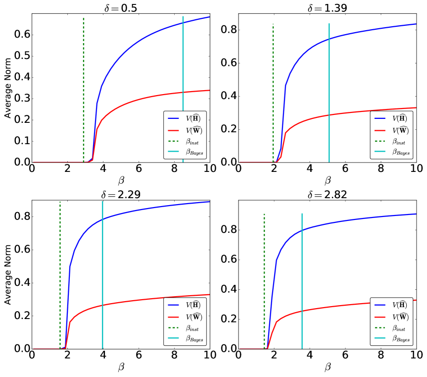
Figure 1: Normalized distances ${\sf V}({\widehat{\boldsymbol{H}}})$, ${\sf V}(\widehat{\boldsymbol{W}})$ of the naive mean field estimates from the uninformative fixed point. Here $k=2$, $d=1000$ and $n=d\delta$: each data point corresponds to an average over $400$ random realizations.

A

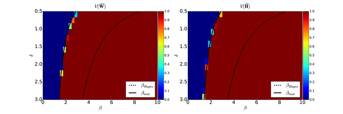
Figure 2: Empirical fraction of instances such that ${\sf V}(\widehat{\boldsymbol{W}})\geq{\varepsilon}_{0}=10^{-4}$ (left frame) or ${\sf V}({\widehat{\boldsymbol{H}}})\geq{\varepsilon}_{0}$ (right frame), where $\widehat{\boldsymbol{W}},{\widehat{\boldsymbol{H}}}$ are the naive mean field estimate. Here $k=2$, $d=1000$ and, for each $(\delta,\beta)$ point on a grid, we used $400$ random realizations to estimate the probability of ${\sf V}(\widehat{\boldsymbol{W}})\geq{\varepsilon}_{0}$.

Recall the definition ${\boldsymbol{P}}_{\perp}={\boldsymbol{I}}_{k}-{\boldsymbol{1}}_{k}{\boldsymbol{1}}_{k}^{{\sf T}}/k$. In order to investigate the instability of Theorem 2, we define the quantities

$${\sf V}(\widehat{\boldsymbol{W}})\equiv\frac{1}{\sqrt{n}}\,\|\widehat{\boldsymbol{W}}{\boldsymbol{P}}_{\perp}\|_{F}\,,\;\;\;\;\;\;{\sf V}({\widehat{\boldsymbol{H}}})\equiv\frac{1}{\sqrt{d}}\,\|{\widehat{\boldsymbol{H}}}{\boldsymbol{P}}_{\perp}\|_{F}$$ (3.28)

In Figure 1 we plot empirical results for the average ${\sf V}(\widehat{\boldsymbol{W}})$, ${\sf V}({\widehat{\boldsymbol{H}}})$ for $k=2$, $\nu=1$ and four values of $\delta$. In Figure 2, we plot the empirical probability that variational inference does not converge to the uninformative fixed point or, more precisely, $\widehat{\mathbb{P}}({\sf V}(\widehat{\boldsymbol{W}})\geq{\varepsilon}_{0})$ with ${\varepsilon}_{0}=10^{-4}$, evaluated on a grid of $(\beta,\delta)$ values. We also plot the Bayes threshold $\beta_{\mbox{\tiny\rm Bayes}}$ (which we find numerically that it coincides with the spectral threshold $\beta_{\mbox{\tiny\rm spect}}$) and the instability threshold $\beta_{\mbox{\tiny\rm inst}}$.

It is clear from Figures 1, 2, that variational inference stops converging to the uninformative fixed point (although we initialize close to it) when $\beta$ is still significantly smaller than the Bayes threshold $\beta_{\mbox{\tiny\rm Bayes}}$ (i.e. in a regime in which the uninformative fixed point would a reasonable output). The data are consistent with the hypothesis that variational inference becomes unstable at $\beta_{\mbox{\tiny\rm inst}}$, as predicted by Theorem 2.

A

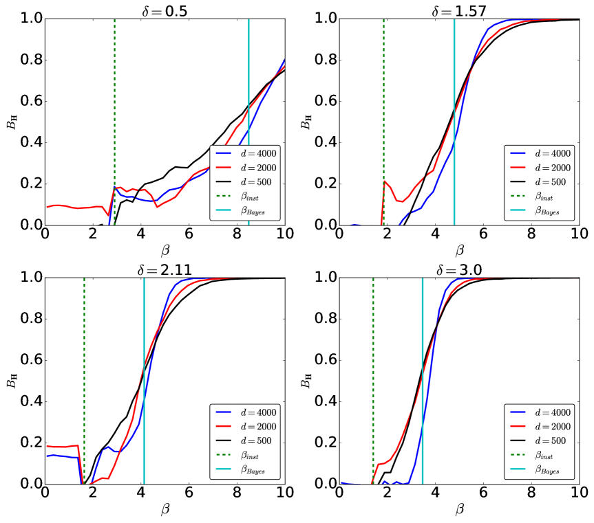
Figure 3: Binder cumulant for the correlation between the naive mean field estimates ${\widehat{\boldsymbol{H}}}$ and the true topics ${\boldsymbol{H}}$, see Eq. (3.29). Here we report results for $k=2$, $d\in\{500,2000,4000\}$ and $n=d\delta$, obtained by averaging over $400$ realizations. Note that for $\beta<\beta_{\mbox{\tiny\rm Bayes}}(k,\nu,\delta)$, ${\sf B}_{{\boldsymbol{H}}}$ decreases with increasing dimensions, suggesting asymptotically vanishing correlations.

A

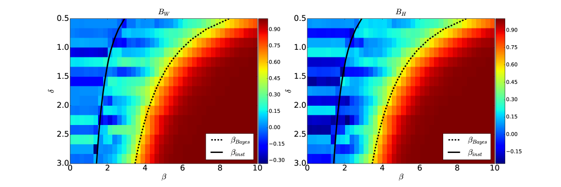
Figure 4: Binder cumulant for the correlation between the naive mean field estimates $\widehat{\boldsymbol{W}}$, ${\widehat{\boldsymbol{H}}}$ and the true weights and topics ${\boldsymbol{W}}$, ${\boldsymbol{H}}$. Here $k=2$, $d=1000$ and $n=d\delta$, and we averaged over $400$ realizations.

Because of Proposition 3.1, we expect the estimates ${\widehat{\boldsymbol{H}}},\widehat{\boldsymbol{W}}$ produced by variational inference to be asymptotically uncorrelated with the true factors for $\beta_{\mbox{\tiny\rm inst}}<\beta<\beta_{\mbox{\tiny\rm Bayes}}$. In order to test this hypothesis, we borrow a technique that has been developed in the study of phase transitions in statistical physics, and is known as the Binder cumulant [Bin81]. For the sake of simplicity, we focus here –again– on the case $k=2$, deferring the general case to Appendix E. Since in this case ${\widehat{\boldsymbol{H}}},{\boldsymbol{H}}\in\mathbb{R}^{d\times 2}$, $\widehat{\boldsymbol{W}},{\boldsymbol{W}}\in\mathbb{R}^{n\times 2}$, we can encode the informative component of these matrices by taking the difference between their columns. For instance, we define $\widehat{\boldsymbol{h}}_{\perp}\equiv{\widehat{\boldsymbol{H}}}({\boldsymbol{e}}_{1}-{\boldsymbol{e}}_{2})$, and analogously ${\boldsymbol{h}}_{\perp}$, $\widehat{\boldsymbol{w}}_{\perp}$, ${\boldsymbol{w}}_{\perp}$. We then define

$${\sf C}_{\eta}({\boldsymbol{H}},{\widehat{\boldsymbol{H}}}) \equiv\langle\widehat{\boldsymbol{h}}_{\perp}+\eta{\boldsymbol{g}},{\boldsymbol{h}}_{\perp}\rangle\,,\;\;\;\;\;\;\;\;{\sf B}_{{\boldsymbol{H}}}\equiv\frac{3}{2}-\frac{\widehat{\mathbb{E}}\{{\sf C}_{\eta}({\boldsymbol{H}},{\widehat{\boldsymbol{H}}})^{4}\}}{2\widehat{\mathbb{E}}\{{\sf C}_{\eta}({\boldsymbol{H}},{\widehat{\boldsymbol{H}}})^{2}\}^{2}}\,.$$ (3.29)

Here $\widehat{\mathbb{E}}$ denotes empirical average with respect to the sample, ${\boldsymbol{g}}\sim{\sf N}(0,{\boldsymbol{I}}_{d})$, and we set $\eta=10^{-4}$. An analogous definition holds for ${\sf C}_{\eta}(\widehat{\boldsymbol{W}})$, ${\sf B}_{\eta}(\widehat{\boldsymbol{W}})$.

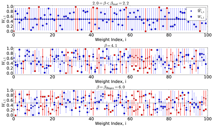
Figure 5: Bayesian credible intervals as computed by variational inference at nominal coverage level $1-\alpha=0.9$. Here $k=2$, $n=d=5000$, and we consider three values of $\beta$: $\beta\in\{2,4.1,6\}$ (for reference $\beta_{\mbox{\tiny\rm inst}}\approx 2.2,\beta_{\mbox{\tiny\rm Bayes}}=6$). Circles correspond to the posterior mean, and squares to the actual weights. We use red for the coordinates on which the credible interval does not cover the actual value of $w_{i,1}$.

The rationale for definition (3.29) is easy to explain. At small signal-to-noise ratio $\beta$, we expect $\widehat{\boldsymbol{h}}_{\perp}$ to be essentially uncorrelated from ${\boldsymbol{h}}_{\perp}$ and hence the correlation ${\sf C}_{\eta}({\boldsymbol{H}},{\widehat{\boldsymbol{H}}})$ to be roughly normal with mean zero and variance $\sigma^{2}_{{\boldsymbol{H}}}$. In particular ${\mathbb{E}}\{{\sf C}_{\eta}({\boldsymbol{H}},{\widehat{\boldsymbol{H}}})^{4}\}\approx 3{\mathbb{E}}\{{\sf C}_{\eta}({\boldsymbol{H}},{\widehat{\boldsymbol{H}}})^{4}\}$ and therefore ${\sf B}_{{\boldsymbol{H}}}\approx 0$. (Note that the term $\eta{\boldsymbol{g}}$ is added to avoid that empirical correlation vanishes, and hence ${\sf B}_{{\boldsymbol{H}}}$ is not defined.)

In contrast, for large $\beta$, we expect $\widehat{\boldsymbol{h}}_{\perp}$ to be positively correlated with ${\boldsymbol{h}}_{\perp}$, and ${\sf C}_{\eta}({\boldsymbol{H}},{\widehat{\boldsymbol{H}}})$ should concentrate around a non-random positive value. As a consequence, ${\sf B}_{{\boldsymbol{H}}}\approx 1$.

In Figures 3 we report our empirical results for ${\sf B}_{{\boldsymbol{H}}}$ and ${\sf B}_{{\boldsymbol{W}}}$ for four different values of $\delta$, and several values of $d$. As expected, these quantities grow from $0$ to $1$ as $\beta$ grows, and the transition is centered around $\beta_{\mbox{\tiny\rm Bayes}}$. Figure 4 reports the results on a grid of $(\beta,\delta)$ values. Again, the transition is well predicted by the analytical curve $\beta_{\mbox{\tiny\rm Bayes}}$. These data support our claim that, for $\beta_{\mbox{\tiny\rm inst}}<\beta<\beta_{\mbox{\tiny\rm Bayes}}$, the output of variational inference is non-uniform but uncorrelated with the true signal.

Finally, in Figure 5 we plot the estimates obtained for $100$ entries of the weights vector $w_{i,1}$ for three instances with $n=d=5000$ and $\beta=2<\beta_{\mbox{\tiny\rm inst}}$, $\beta=4.1\in(\beta_{\mbox{\tiny\rm inst}},\beta_{\mbox{\tiny\rm Bayes}})$ and $\beta=6=\beta_{\mbox{\tiny\rm Bayes}}$. The interval for $w_{a,1}$ is the form $\{w_{a,1}\in[0,1]:\tilde{q}_{a}(w_{a,1})\geq t_{a}(\alpha)\}$ and are constructed to achieve nominal coverage level $1-\alpha=0.9$. It is visually clear that the claimed coverage level is not verified in these simulations for $\beta>\beta_{\mbox{\tiny\rm inst}}$, confirming our analytical results. Indeed, for the three simulations in Figure 5 we achieve coverage $0.87$ (for $\beta=2<\beta_{\mbox{\tiny\rm inst}}$), $0.65$ (for $\beta=4.1\in(\beta_{\mbox{\tiny\rm inst}},\beta_{\mbox{\tiny\rm Bayes}})$), and $0.51$ (for $\beta=6=\beta_{\mbox{\tiny\rm Bayes}}$). Further results of this type are reported in Appendix E.

4 Fixing the instability

The fact that naive mean field is not accurate for certain classes of random high-dimensional probability distributions is well understood within statistical physics. In particular, in the context of mean field spin glasses [MPV87], naive mean field is known to lead to an asymptotically incorrect expression for the free energy. We expect the same mechanism to be relevant in the context of topic models.

Namely, the product-form expression (1.5) only holds asymptotically in the sense of finite-dimensional marginals. However, when computing the term ${\mathbb{E}}_{\hat{q}}\log p_{\boldsymbol{X}|{\boldsymbol{W}},{\boldsymbol{H}}}(\boldsymbol{X}|{\boldsymbol{H}},{\boldsymbol{W}})$ in the KL divergence (1.4), the error due to the product form approximation is non-negligible. Keeping track of this error leads to the so-called TAP free energy.

4.1 Revisiting ${\mathbb{Z}}_{2}$-synchronization

It is instructive to briefly discuss the ${\mathbb{Z}}_{2}$-synchronization example of Section 2, as the basic concepts can be explained more easily in this example. For this problem, the TAP approximation replaces the free energy (2.4) with

$${\cal F}_{\mbox{\tiny\rm TAP}}({\boldsymbol{m}}) \equiv-\frac{\lambda}{2}\langle{\boldsymbol{m}},\boldsymbol{X}_{0}{\boldsymbol{m}}\rangle-\sum_{i=1}^{n}{\sf h}(m_{i})-\frac{n\lambda^{2}}{4}\big{(}1-Q({\boldsymbol{m}})\big{)}^{2}\,,$$ (4.1)

where $Q({\boldsymbol{m}})\equiv\|{\boldsymbol{m}}\|_{2}^{2}/n$.

We can now repeat the analysis of Section 2 with this new free energy approximation. It is easy to see that ${\boldsymbol{m}}_{*}={\boldsymbol{0}}$ is again a stationary point. However, the Hessian is now

$$\left.\nabla^{2}{\cal F}({\boldsymbol{m}})\right|_{{\boldsymbol{m}}={\boldsymbol{m}}_{*}}=-\lambda\boldsymbol{X}_{0}+\left(1+\lambda^{2}\right){\boldsymbol{I}}\,.$$ (4.2)

In particular, for $\lambda<1$, $\lambda_{\rm min}(\left.\nabla^{2}{\cal F}\right|_{{\boldsymbol{m}}={\boldsymbol{m}}_{*}})$ converges to $(1-\lambda)^{2}>0$: the uninformative stationary point is (with high probability) a local minimum.

The stationarity condition for the TAP free energy are known as TAP equations, and the algorithm that corresponds to the naive mean field iteration is Bayesian approximate message passing (AMP). For the ${\mathbb{Z}}_{2}$ synchronization problem, Bayes AMP is known to achieve the Bayes optimal estimation error [DAM17, MV17].

4.2 TAP free energy for topic models

We now turn to topic models. The TAP approach replaces the free energy (3.9) with the following (see Appendix F.1 for a derivation)

$${\cal F}_{\mbox{\tiny\rm TAP}}({\boldsymbol{r}},\tilde{\boldsymbol{r}})= \sum_{i=1}^{d}\psi\left({\boldsymbol{r}}_{i},\frac{\beta}{d}\sum_{a=1}^{n}\tilde{\boldsymbol{r}}_{a}^{\otimes 2}\right)+\sum_{a=1}^{n}{\tilde{\psi}}\left(\tilde{\boldsymbol{r}}_{a},\frac{\beta}{d}\sum_{i=1}^{d}{\boldsymbol{r}}_{i}^{\otimes 2}\right)-\sqrt{\beta}{\sf{Tr}}\left(\boldsymbol{X}{\boldsymbol{r}}\tilde{\boldsymbol{r}}^{{\sf T}}\right)-\frac{\beta}{2d}\sum_{i=1}^{d}\sum_{a=1}^{n}\langle{\boldsymbol{r}}_{i},\tilde{\boldsymbol{r}}_{a}\rangle^{2}\,,$$ (4.3)

where $\tilde{\boldsymbol{r}}{\boldsymbol{1}}_{k}={\boldsymbol{1}}_{n}$, and we defined the partial Legendre transforms

$$\psi({\boldsymbol{r}},{\boldsymbol{Q}})\equiv\sup_{{\boldsymbol{m}}}\left\{\langle{\boldsymbol{r}},{\boldsymbol{m}}\rangle-\phi({\boldsymbol{m}},{\boldsymbol{Q}})\right\}\,,\;\;\;\;{\tilde{\psi}}(\tilde{\boldsymbol{r}},\widetilde{\boldsymbol{Q}})\equiv\sup_{\tilde{\boldsymbol{m}}}\left\{\langle\tilde{\boldsymbol{r}},\tilde{\boldsymbol{m}}\rangle-{\tilde{\phi}}(\tilde{\boldsymbol{m}},\widetilde{\boldsymbol{Q}})\right\}\,.$$ (4.4)

Notice that ${\tilde{\psi}}(\tilde{\boldsymbol{r}},\widetilde{\boldsymbol{Q}})$ is finite only if $\langle{\boldsymbol{1}}_{k},\tilde{\boldsymbol{r}}\rangle=1$.

When substituting in Eq. (4.3), the supremum of Eq. (4.4) is achieved at

$${\boldsymbol{r}} =\frac{1}{\sqrt{\beta}}{\sf F}({\boldsymbol{m}};{\boldsymbol{Q}})\,,\;\;\;\;\;\tilde{\boldsymbol{r}}=\frac{1}{\sqrt{\beta}}\widetilde{\sf F}(\tilde{\boldsymbol{m}};\widetilde{\boldsymbol{Q}})\,,$$ (4.5)

$${\boldsymbol{Q}} =\frac{\beta}{d}\sum_{a=1}^{n}\tilde{\boldsymbol{r}}_{a}^{\otimes 2},\;\;\;\;\;\;\widetilde{\boldsymbol{Q}}\equiv\frac{\beta}{d}\sum_{i=1}^{d}{\boldsymbol{r}}_{i}^{\otimes 2}\,.$$ (4.6)

Calculus shows that stationary points of this free energy are in one-to-one correspondence (via Eq. (4.5)) with the fixed points of the following iteration:

$${\boldsymbol{m}}^{t+1} =\boldsymbol{X}^{{\sf T}}\,\widetilde{\sf F}(\tilde{\boldsymbol{m}}^{t};\widetilde{\boldsymbol{Q}}^{t})-{\sf F}({\boldsymbol{m}}^{t};{\boldsymbol{Q}}^{t})\tilde{\boldsymbol{\Omega}}_{t}\,,$$ (4.7)

$$\tilde{\boldsymbol{m}}^{t} =\boldsymbol{X}\,{\sf F}({\boldsymbol{m}}^{t};{\boldsymbol{Q}}^{t})-\widetilde{\sf F}(\tilde{\boldsymbol{m}}^{t-1};\widetilde{\boldsymbol{Q}}^{t-1}){\boldsymbol{\Omega}}_{t}\,,$$ (4.8)

$${\boldsymbol{Q}}^{t+1} =\frac{1}{d}\sum_{a=1}^{n}\widetilde{\sf F}(\tilde{\boldsymbol{m}}^{t}_{a};\widetilde{\boldsymbol{Q}}^{t})^{\otimes 2}\,,\;\;\;\;\widetilde{\boldsymbol{Q}}^{t}=\frac{1}{d}\sum_{i=1}^{d}{\sf F}({\boldsymbol{m}}^{t}_{i};{\boldsymbol{Q}}^{t})^{\otimes 2}\,.$$ (4.9)

where ${\boldsymbol{\Omega}}_{t}$, $\tilde{\boldsymbol{\Omega}}_{t}$ are defined as

$${\boldsymbol{\Omega}}_{t} =\frac{1}{d\sqrt{\beta}}\sum_{i=1}^{d}[{\sf G}({\boldsymbol{m}}^{t}_{i},{\boldsymbol{Q}}^{t})-{\sf F}({\boldsymbol{m}}^{t}_{i};{\boldsymbol{Q}}^{t})^{\otimes 2}]=\frac{1}{d}\sum_{i=1}^{d}\frac{\partial{\sf F}}{\partial{\boldsymbol{m}}_{i}}({\boldsymbol{m}}^{t}_{i};{\boldsymbol{Q}}^{t})\,,$$ (4.10)

$$\tilde{\boldsymbol{\Omega}}_{t} =\frac{1}{d\sqrt{\beta}}\sum_{a=1}^{n}[\widetilde{\sf G}(\tilde{\boldsymbol{m}}^{t}_{a},\widetilde{\boldsymbol{Q}})-\widetilde{\sf F}(\tilde{\boldsymbol{m}}^{t}_{a};\widetilde{\boldsymbol{Q}}^{t})^{\otimes 2}]=\frac{1}{d}\sum_{a=1}^{n}\frac{\partial\widetilde{\sf F}}{\partial\tilde{\boldsymbol{m}}_{a}}(\tilde{\boldsymbol{m}}^{t}_{a};\widetilde{\boldsymbol{Q}}^{t})\,.$$ (4.11)

The stationarity conditions for the TAP free energy (4.3) are known as TAP equations, and the corresponding iterative algorithm (4.7), (4.8) is a special case of approximate message passing (AMP), with Bayesian updates. Note that the specific choice of time indices in Eqs.  (4.7), (4.8) is instrumental for the analysis in the next section to hold. We also note that the general AMP analysis of [BM11, JM13] allows for quite general choices of the sequence of matrices ${\boldsymbol{Q}}_{t},\widetilde{\boldsymbol{Q}}_{t}$. However, stationarity of the TAP free energy (4.3) requires that at convergence the condition (4.9) holds at the fixed point

Estimates of the factors ${\boldsymbol{W}}$, ${\boldsymbol{H}}$ are computed following the same recipe as for naive mean field, cf. Eq. (3.24), namely ${\widehat{\boldsymbol{H}}}^{t}={\boldsymbol{r}}^{t}={\sf F}({\boldsymbol{m}}^{t};{\boldsymbol{Q}}_{t})/\sqrt{\beta}$, $\widehat{\boldsymbol{W}}^{t}=\tilde{\boldsymbol{r}}^{t}=\widetilde{\sf F}(\tilde{\boldsymbol{m}}^{t};\widetilde{\boldsymbol{Q}}_{t})/\sqrt{\beta}$.

It is not hard to see that the AMP iteration admits an uninformative fixed point, which is a stationary point of the TAP free energy, see proof in Appendix F.3.

Lemma 4.1.

Define $q_{0}^{*}=\beta\delta/k^{2}$ and $\tilde{q}_{0}^{*}=\beta^{2}\|\boldsymbol{X}^{{\sf T}}{\boldsymbol{1}}_{n}\|_{2}^{2}/(dk^{2}(1+kq_{0})^{2})$. Then, AMP iteration admits the following fixed point

$${\boldsymbol{m}}^{*} =\frac{\sqrt{\beta}}{k}(\boldsymbol{X}^{{\sf T}}{\boldsymbol{1}}_{n})\otimes{\boldsymbol{1}}_{k}\,,$$ (4.12)

$$\tilde{\boldsymbol{m}}^{*} =\frac{\beta}{k(1+kq_{0})}(\boldsymbol{X}\boldsymbol{X}^{{\sf T}}{\boldsymbol{1}}_{n})\otimes{\boldsymbol{1}}_{k}-\frac{\beta}{k+\delta\beta}\,{\boldsymbol{1}}_{n}\otimes{\boldsymbol{1}}_{k}\,,$$ (4.13)

$${\boldsymbol{Q}}^{*} =q_{0}^{*}\,{\boldsymbol{J}}_{k}\,,\;\;\;\;\;\;\;\;\widetilde{\boldsymbol{Q}}^{*}=\tilde{q}_{0}^{*}\,{\boldsymbol{J}}_{k}\,.$$ (4.14)

This corresponds to a stationary point of the TAP free energy (4.3), via Eq. (4.5):

$${\boldsymbol{r}}_{*}=\frac{\sqrt{\beta}}{k(1+kq_{0}^{*})}(\boldsymbol{X}^{{\sf T}}{\boldsymbol{1}}_{n})\otimes{\boldsymbol{1}}_{k}\,,\;\;\;\;\;\;\;\tilde{\boldsymbol{r}}_{*}=\frac{1}{k}{\boldsymbol{1}}_{n}\otimes{\boldsymbol{1}}_{k}\,.$$ (4.15)

Further, this is the only stationary point that is unchanged under permutations of the topics.

4.3 State evolution analysis

State evolution is a recursion over matrices ${\boldsymbol{M}}_{t}$, $\widetilde{\boldsymbol{M}}_{t}\in\mathbb{R}^{k\times k}$, defined by

$${\boldsymbol{M}}_{t+1} =\delta\,{\mathbb{E}}\Big{\{}\widetilde{\sf F}(\widetilde{\boldsymbol{M}}_{t}{\boldsymbol{w}}+\widetilde{\boldsymbol{M}}_{t}^{1/2}{\boldsymbol{z}};\widetilde{\boldsymbol{M}}_{t})^{\otimes 2}\Big{\}}\,,$$ (4.16)

$$\widetilde{\boldsymbol{M}}_{t} ={\mathbb{E}}\Big{\{}{\sf F}({\boldsymbol{M}}_{t}{\boldsymbol{h}}+{\boldsymbol{M}}_{t}^{1/2}{\boldsymbol{z}};{\boldsymbol{M}}_{t})^{\otimes 2}\Big{\}}\,,$$ (4.17)

where expectation is with respect to ${\boldsymbol{h}}\sim q_{0}(\,\cdot\,)$, ${\boldsymbol{w}}\sim\tilde{q}_{0}(\,\cdot\,)$ and ${\boldsymbol{z}}\sim{\sf N}(0,{\boldsymbol{I}}_{k})$ independent. Note that ${\boldsymbol{M}}_{t},\widetilde{\boldsymbol{M}}_{t}$ are positive semidefinite symmetric matrices. Also, Eq. (4.17) can be written explicitly as

$$\widetilde{\boldsymbol{M}}_{t}=\beta({\boldsymbol{I}}_{k}+{\boldsymbol{M}}_{t})^{-1}{\boldsymbol{M}}_{t}\,.$$ (4.18)

State evolution provides an asymptotically exact characterization of the behavior of AMP, as formalized by the next theorem (which is a direct application of [JM13]).

Theorem 3.

Consider the AMP algorithm of Eqs. (4.7), with deterministic initialization ${\boldsymbol{m}}^{0},{\boldsymbol{Q}}^{0}$. Assume ${\boldsymbol{G}}\in\mathbb{R}^{d\times k}$ to be independent of data $\boldsymbol{X}$, with entries $(G_{ij})_{i\leq d,j\leq k}\sim_{iid}{\sf N}(0,1)$, and let ${\boldsymbol{m}}^{0}={\boldsymbol{H}}{\boldsymbol{M}}_{0}+{\boldsymbol{Z}}{\boldsymbol{M}}_{0}^{1/2}$ for ${\boldsymbol{M}}_{0}\in\mathbb{R}^{k\times k}$ non-random, ${\boldsymbol{M}}_{0}\succeq 0$. Let $\{{\boldsymbol{M}}_{t},\widetilde{\boldsymbol{M}}_{t}\}_{t\geq 1}$ be defined by the state evolution recursion (4.16), (4.17). Then, for any pseudo-Lipschitz function $g:\mathbb{R}^{k}\times\mathbb{R}^{k}\to\mathbb{R}$, we have, almost surely,

$$\lim_{n\to\infty}\frac{1}{d}\sum_{i=1}^{d}g({\boldsymbol{h}}_{i},{\boldsymbol{m}}^{t}_{i}) ={\mathbb{E}}\Big{\{}g({\boldsymbol{h}},{\boldsymbol{M}}_{t}{\boldsymbol{h}}+{\boldsymbol{M}}_{t}^{1/2}{\boldsymbol{z}})\Big{\}}\,,$$ (4.19)

$$\lim_{n\to\infty}\frac{1}{n}\sum_{a=1}^{n}g({\boldsymbol{w}}_{a},\tilde{\boldsymbol{m}}^{t}_{a}) ={\mathbb{E}}\Big{\{}g({\boldsymbol{w}},\widetilde{\boldsymbol{M}}_{t}{\boldsymbol{w}}+\widetilde{\boldsymbol{M}}_{t}^{1/2}{\boldsymbol{z}})\Big{\}}\,,$$ (4.20)

where it is understood that $n,d\to\infty$ with $n/d\to\delta$. In particular

$$\lim_{n\to\infty}\frac{1}{d}{\boldsymbol{H}}^{{\sf T}}{\widehat{\boldsymbol{H}}}^{t} =\frac{1}{\sqrt{\beta}}\widetilde{\boldsymbol{M}}_{t}\,,$$ (4.21)

$$\lim_{n\to\infty}\frac{1}{n}{\boldsymbol{W}}^{{\sf T}}\widehat{\boldsymbol{W}}^{t} =\frac{1}{\sqrt{\beta}}{\boldsymbol{M}}_{t+1}\,.$$ (4.22)

Further $\lim_{n\to\infty}{\boldsymbol{Q}}^{t}={\boldsymbol{M}}_{t}$, $\lim_{n\to\infty}\widetilde{\boldsymbol{Q}}^{t}=\widetilde{\boldsymbol{M}}_{t}$.

Using state evolution, we can establish a stability result for AMP. First of all, notice that the state evolution iteration (4.16), (4.17) admits a fixed point of the form ${\boldsymbol{M}}^{*}=(\delta\beta/k^{2}){\boldsymbol{J}}_{k}$, $\widetilde{\boldsymbol{M}}^{*}=\rho_{0}{\boldsymbol{J}}_{k}$, for $\rho_{0}=\delta\beta^{2}/(k\delta\beta+k^{2})$, see Appendix G.2. This is an uninformative fixed point, in the sense that the $k$ topics are asymptotically identical. The next theorem is proved in Appendix G.3.

Theorem 4.

If $\beta<\beta_{\mbox{\tiny\rm spect}}(k,\nu,\delta)$, then the uninformative fixed point is stable under the state evolution iteration (4.16), (4.17).

In particular, for $\beta<\beta_{\mbox{\tiny\rm spect}}(k,\nu,\delta)$, there exists $c_{0}=c_{0}(\beta,k\nu,\delta)$ such that, if we initialize AMP as in Theorem 3 with $\|{\boldsymbol{M}}_{0}-{\boldsymbol{M}}^{*}\|_{F}\leq c_{0}$, then (recalling ${\boldsymbol{P}}_{\perp}={\boldsymbol{I}}_{k}-{\boldsymbol{1}}_{k}{\boldsymbol{1}}_{k}/k$)

$$\lim_{t\to\infty}\lim_{n\to\infty}\frac{1}{n}\big{\|}{\boldsymbol{m}}^{t}{\boldsymbol{P}}_{\perp}\|_{F}^{2}=0\,,\;\;\;\;\;\;\lim_{t\to\infty}\lim_{n\to\infty}\frac{1}{n}\big{\|}{\boldsymbol{m}}^{t}{\boldsymbol{P}}_{\perp}\|_{F}^{2}=0\,.$$ (4.23)

4.4 Stability of the uninformative fixed point

The next theorem establishes that the uninformative fixed point of the TAP free energy is a local minimum for all $\beta$ below the spectral threshold $\beta_{\mbox{\tiny\rm spect}}(k,\nu,\delta)$. Since $\beta_{\mbox{\tiny\rm Bayes}}(k,\nu,\delta)\leq\beta_{\mbox{\tiny\rm spect}}(k,\nu,\delta)$, this shows that the instability we discovered in the case of naive mean field is corrected by the TAP free energy.

Theorem 5.

Let $({\boldsymbol{r}}_{*},\tilde{\boldsymbol{r}}_{*})$ be the uninformative stationary point of the TAP free energy, cf. Lemma 4.1. If $\beta<\beta_{\mbox{\tiny\rm spect}}(k,\nu,\delta)$, then there exists ${\varepsilon}>0$ such that, with high probability

$$\lambda_{\min}\left(\left.\nabla^{2}{\cal F}_{\mbox{\tiny\rm TAP}}\right|_{({\boldsymbol{r}}_{*},\tilde{\boldsymbol{r}}_{*})}\right)\geq{\varepsilon}\,.$$ (4.24)

Remark 4.1.

Let us emphasize that this result is not implied by the state evolution result of Theorem 4, which only establishes stability in a certain asymptotic sense. Vice-versa, Theorem 5 does not directly imply Theorem 4.

4.5 Numerical results for TAP free energy

A

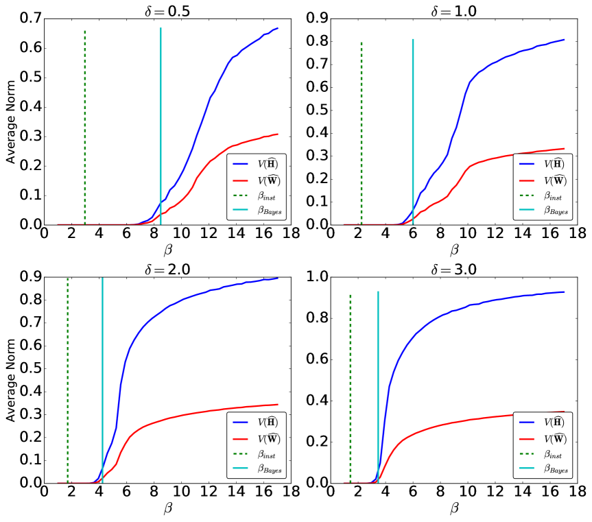
Figure 6: Normalized distances ${\sf V}({\widehat{\boldsymbol{H}}})$, ${\sf V}(\widehat{\boldsymbol{W}})$ of the AMP estimates from the uninformative fixed point. Here, $k=2$, $d=1000$ and $n=d\delta$: each data point corresponds to an average over $400$ random realizations.

A

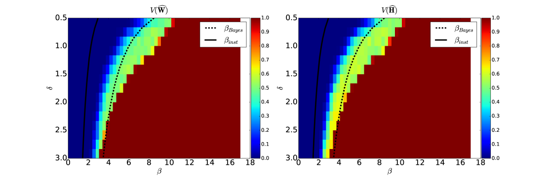
Figure 7: Empirical fraction of instances such that ${\sf V}(\widehat{\boldsymbol{W}})\geq{\varepsilon}_{0}=5\cdot 10^{-3}$, where $\widehat{\boldsymbol{W}}$ is the AMP estimate. Here $k=2$, $d=1000$, and for each $(\delta,\beta)$ point on the grid we ran AMP on $400$ random realizations.

A

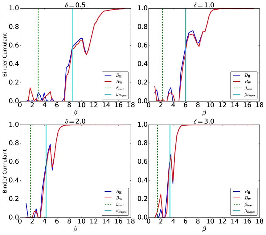
Figure 8: Binder cumulant for the correlation between AMP estimates ${\widehat{\boldsymbol{H}}}$ and the true topics ${\boldsymbol{H}}$, and between $\widehat{\boldsymbol{W}}$ and ${\boldsymbol{W}}$, see Eq. (3.29). Here $k=2$, $d=1000$, $n=d\delta$ and estimates are obtained by averaging over $400$ realizations.

A

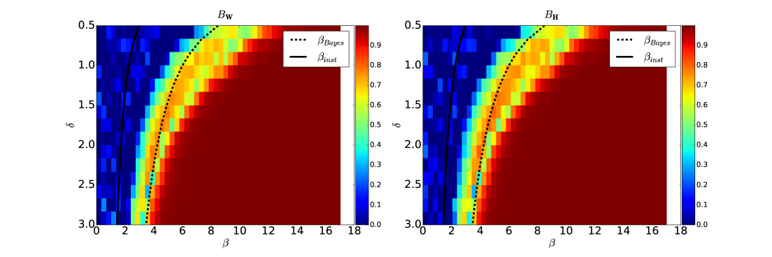
Figure 9: Binder cumulant for the correlation between AMP estimates $\widehat{\boldsymbol{W}}$, ${\widehat{\boldsymbol{H}}}$ and the true weights and topics ${\boldsymbol{W}},{\boldsymbol{H}}$. Here $k=2$,$d=1000$ and estimates are obtained by averaging over $400$ realizations.

In order to confirm the stability analysis at the previous section, we carried out numerical simulations analogous to the ones of Section 3.5. We found that the AMP iteration of Eqs. (4.7), (4.8) is somewhat unstable when $\beta\approx\beta_{\mbox{\tiny\rm spect}}$. In order to remedy this problem, we used a damped version of the same iteration, see Appendix H.1. Notice that damping does not change the stability of a local minimum or saddle, it merely reduces oscillations due to aggressive step sizes.

We initialize the iteration as for naive mean field, and monitor the same quantities, as in Section 3.5. In particular, here we report results on the distance from the uninformative subspace ${\sf V}({\widehat{\boldsymbol{H}}})$, ${\sf V}(\widehat{\boldsymbol{W}})$, in Figures 6 and 7, and the Binder cumulants ${\sf B}_{{\boldsymbol{H}}}$ and ${\sf B}_{{\boldsymbol{W}}}$, measuring the correlation between AMP estimates and the true factors ${\boldsymbol{W}},{\boldsymbol{H}}$, in Figures 8, 9. We focus on the case $k=2$, deferring $k=3$ to the appendices.

In the intermediate regime $\beta\in(\beta_{\mbox{\tiny\rm inst}},\beta_{\mbox{\tiny\rm spect}})$, the behavior of AMP is strikingly different from the one of naive mean field. AMP remains close to the uninformative fixed point, confirming that this is a local minimum of the TAP free energy. The distance from the uninformative subspace starts growing only at the spectral threshold $\beta_{\mbox{\tiny\rm spect}}$ (which coincides, in the present cases, with the Bayes threshold $\beta_{\mbox{\tiny\rm Bayes}}$). At the same point, the correlation with the true factors ${\boldsymbol{W}}$, ${\boldsymbol{H}}$ also becomes strictly positive.

5 Discussion

Bayesian methods are particularly attractive in unsupervised learning problems such as topic modeling. Faced with a collection of documents ${\boldsymbol{x}}_{1}$,…${\boldsymbol{x}}_{n}$, it is not clear a priori whether they should be modeled as convex combinations of topics, or how many topics should be used. Even after a low-rank factorization $\boldsymbol{X}\approx{\boldsymbol{W}}{\boldsymbol{H}}^{{\sf T}}$ is computed, it is still unclear how to evaluate it, or to which extent it should be trusted.

Bayesian approaches provide estimates of the factors ${\boldsymbol{W}}$, ${\boldsymbol{H}}$, but also a probabilistic measure of how much these estimates should be trusted. To the extent that the posterior concentrates around its mean, this can be considered as a good estimate of a true underlying signal.

It is well understood that Bayesian estimates can be unreliable if the prior is not chosen carefully. Our work points at a second reason for caution. When variational inference is used for approximating the posterior, the result can be incorrect even if the data are generated according to the prior. More precisely, we showed that for a certain regime of parameters, naive mean field ‘believes’ that there is a signal, even if it is information-theoretically impossible to extract any non-trivial estimate from the data.

Given that naive mean field is the method of choice for inference with topic models [BNJ03], it would be of great interest to remedy this instability. We showed that the TAP free energy provides a better mean field approximation, and in particular does not have the same instability. However, this approximation is also based on the correctness of the generative model, and further investigation is warranted on its robustness.

Appendix A Some remarks on alternating minimization

Let $f:\mathbb{R}^{n}\times\mathbb{R}^{d}\to\mathbb{R}$ be twice continuously differentiable in an open neighborhood $\Omega_{1}\times\Omega_{2}\subseteq\mathbb{R}^{n}\times\mathbb{R}^{d}$ of a critical point $({\boldsymbol{x}}^{*},{\boldsymbol{y}}^{*})$ (i.e. a point for which $\nabla_{({\boldsymbol{x}},{\boldsymbol{y}})}f({\boldsymbol{x}},{\boldsymbol{y}})={\boldsymbol{0}}$). Further assume that, fixing ${\boldsymbol{x}}_{0}\in\Omega_{1}$, $f({\boldsymbol{x}}_{0},\,\cdot\,)$ is strongly convex with a minimizer in $\Omega_{2}$, and fixing ${\boldsymbol{y}}_{0}\in\Omega_{2}$, $f(\,\cdot\,,{\boldsymbol{y}}_{0})$ is strongly convex with a minimizer in $\Omega_{1}$. By taking $\Omega_{1}$ and $\Omega_{2}$ sufficiently small, these conditions follow by requiring that the partial Hessians satisfy $\nabla^{2}_{{\boldsymbol{x}}}f({\boldsymbol{x}}^{*},{\boldsymbol{y}}^{*})\succ{\boldsymbol{0}}$ and $\nabla^{2}_{{\boldsymbol{y}}}f({\boldsymbol{x}}^{*},{\boldsymbol{y}}^{*})\succ{\boldsymbol{0}}$ (i.e. they are strictly positive definite).

By strong convexity, the minimizers of $f({\boldsymbol{x}}_{0},\,\cdot\,)$ and $f(\,\cdot\,,{\boldsymbol{y}}_{0})$ are unique, and we can define the functions $g:\mathbb{R}^{d}\to\mathbb{R}^{n}$ and $h:\mathbb{R}^{n}\to\mathbb{R}^{d}$ by

$$h({\boldsymbol{x}}_{0})=\arg\min_{{\boldsymbol{y}}\in\Omega_{2}}f({\boldsymbol{x}}_{0},{\boldsymbol{y}})\,,$$ (A.1)

$$g({\boldsymbol{y}}_{0})=\arg\min_{{\boldsymbol{x}}\in\Omega_{1}}f({\boldsymbol{x}},{\boldsymbol{y}}_{0})\,.$$ (A.2)

We then define the alternating minimization iteration

$${\boldsymbol{x}}^{t+1}=h({\boldsymbol{y}}^{t}),\;\;\;\;\;\;{\boldsymbol{y}}^{t}=g({\boldsymbol{x}}^{t})\,.$$ (A.3)

If $d=n$ and $h:\Omega_{1}\to\Omega_{2}$, $g:\Omega_{2}\to\Omega_{1}$ are bijective, we also define the dual iteration

$$\overline{\boldsymbol{x}}^{t+1}=g^{-1}(\overline{\boldsymbol{y}}^{t}),\;\;\;\;\;\;\overline{\boldsymbol{y}}^{t}=h^{-1}(\overline{\boldsymbol{x}}^{t})\,.$$ (A.4)

Lemma A.1.

Let $f:\mathbb{R}^{n}\times\mathbb{R}^{d}\to\mathbb{R}$ by twice continuously differentiable in $\Omega_{1}\times\Omega_{2}$, satisfying the above assumptions. Then the following are equivalent:

• The Hessian ${\boldsymbol{H}}=\nabla^{2}_{({\boldsymbol{x}},{\boldsymbol{y}})}f\big{|}_{({\boldsymbol{x}},{\boldsymbol{y}})=({\boldsymbol{x}}^{*},{\boldsymbol{y}}^{*})}$ is strictly positive definite.

• $({\boldsymbol{x}}^{*},{\boldsymbol{y}}^{*})$ is a stable fixed point of the alternate minimization algorithm (A.3).

• $f_{1}({\boldsymbol{x}})\equiv\min_{{\boldsymbol{y}}\in\Omega_{2}}f({\boldsymbol{x}},{\boldsymbol{y}})$ is strongly convex in a neighborhood of ${\boldsymbol{x}}^{*}$ (and in particular, ${\boldsymbol{x}}^{*}$ is a local minimum of $f_{1}$).

Further, if $n=d$ and the matrix $\left.\frac{\partial f}{\partial{\boldsymbol{x}}\partial{\boldsymbol{y}}}\right|_{{\boldsymbol{x}}^{*},{\boldsymbol{y}}^{*}}$ is invertible, then the following are equivalent:

• $({\boldsymbol{x}}^{*},{\boldsymbol{y}}^{*})$ is a stable fixed point of the dual algorithm (A.4).

• $f_{1}({\boldsymbol{x}})\equiv\min_{{\boldsymbol{y}}\in\Omega_{2}}f({\boldsymbol{x}},{\boldsymbol{y}})$ is strongly concave in a neighborhood of ${\boldsymbol{x}}^{*}$ (and in particular, ${\boldsymbol{x}}^{*}$ is a local maximum).

Proof.

Let

$${\boldsymbol{H}}=\begin{bmatrix}{\boldsymbol{H}}_{{\boldsymbol{x}}{\boldsymbol{x}}}&{\boldsymbol{H}}_{{\boldsymbol{x}}{\boldsymbol{y}}}\\ {\boldsymbol{H}}_{{\boldsymbol{x}}{\boldsymbol{y}}}^{\sf T}&{\boldsymbol{H}}_{{\boldsymbol{y}}{\boldsymbol{y}}}\end{bmatrix}=\nabla^{2}_{({\boldsymbol{x}},{\boldsymbol{y}})}f\big{|}_{({\boldsymbol{x}},{\boldsymbol{y}})=({\boldsymbol{x}}^{*},{\boldsymbol{y}}^{*})}.$$ (A.5)

(A1)$\equiv$(A2) We compute the linearization of the iterations in (A.3) around the fixed point $({\boldsymbol{x}}^{*},{\boldsymbol{y}}^{*})$. Note that since ${\boldsymbol{x}}^{*}$ is a minimizer of $f(\,\cdot\,,{\boldsymbol{y}}^{*})$, using the implicit function theorem for the Jacobian of the update rule for ${\boldsymbol{x}}$ in (A.3) we have

$$\frac{\partial^{2}f}{\partial{\boldsymbol{x}}\partial{\boldsymbol{y}}}\bigg{|}_{({\boldsymbol{x}},{\boldsymbol{y}})=({\boldsymbol{x}}^{*},{\boldsymbol{y}}^{*})}+\left[\frac{\partial^{2}f}{\partial{\boldsymbol{x}}^{2}}\bigg{|}_{({\boldsymbol{x}},{\boldsymbol{y}})=({\boldsymbol{x}}^{*},{\boldsymbol{y}}^{*})}\right]\left[{\boldsymbol{D}}h({\boldsymbol{y}}^{*})\right]=0.$$ (A.6)

Hence, we get

$${\boldsymbol{D}}h({\boldsymbol{y}}^{*})=-\left[\left(\frac{\partial^{2}f}{\partial{\boldsymbol{x}}^{2}}\right)^{-1}\left(\frac{\partial^{2}f}{\partial{\boldsymbol{x}}\partial{\boldsymbol{y}}}\right)\right]_{({\boldsymbol{x}},{\boldsymbol{y}})=({\boldsymbol{x}}^{*},{\boldsymbol{y}}^{*})}=-{\boldsymbol{H}}_{{\boldsymbol{x}}{\boldsymbol{x}}}^{-1}{\boldsymbol{H}}_{{\boldsymbol{x}}{\boldsymbol{y}}}.$$ (A.7)

Similarly, for the Jacobian of the update rule for ${\boldsymbol{y}}$ in (A.3) we have

$${\boldsymbol{D}}g({\boldsymbol{x}}^{*})=-\left[\left(\frac{\partial^{2}f}{\partial{\boldsymbol{y}}^{2}}\right)^{-1}\left(\frac{\partial^{2}f}{\partial{\boldsymbol{y}}\partial{\boldsymbol{x}}}\right)\right]_{({\boldsymbol{x}},{\boldsymbol{y}})=({\boldsymbol{x}}^{*},{\boldsymbol{y}}^{*})}=-{\boldsymbol{H}}_{{\boldsymbol{y}}{\boldsymbol{y}}}^{-1}{\boldsymbol{H}}_{{\boldsymbol{x}}{\boldsymbol{y}}}^{\sf T}.$$ (A.8)

Hence, $({\boldsymbol{x}}^{*},{\boldsymbol{y}}^{*})$ is stable if and only if the operator

$${\boldsymbol{L}}={\boldsymbol{D}}h({\boldsymbol{x}}^{*})\cdot{\boldsymbol{D}}g({\boldsymbol{y}}^{*})={\boldsymbol{H}}_{{\boldsymbol{x}}{\boldsymbol{x}}}^{-1}{\boldsymbol{H}}_{{\boldsymbol{x}}{\boldsymbol{y}}}{\boldsymbol{H}}_{{\boldsymbol{y}}{\boldsymbol{y}}}^{-1}{\boldsymbol{H}}_{{\boldsymbol{x}}{\boldsymbol{y}}}^{\sf T}\,,$$ (A.9)

has spectral radius

$$\sigma({\boldsymbol{L}})\equiv\max_{i}\left|\lambda_{i}\left({\boldsymbol{L}}\right)\right|<1.$$ (A.10)

Since $f(\,\cdot\,,{\boldsymbol{x}}^{*})$ is strongly convex, the matrices ${\boldsymbol{H}}_{{\boldsymbol{x}}{\boldsymbol{x}}},{\boldsymbol{H}}_{{\boldsymbol{x}}{\boldsymbol{x}}}^{-1}$ are positive definite. Hence, the eigenvalues of ${\boldsymbol{H}}_{{\boldsymbol{x}}{\boldsymbol{x}}}^{-1}{\boldsymbol{H}}_{{\boldsymbol{x}}{\boldsymbol{y}}}{\boldsymbol{H}}_{{\boldsymbol{y}}{\boldsymbol{y}}}^{-1}{\boldsymbol{H}}_{{\boldsymbol{x}}{\boldsymbol{y}}}^{\sf T}$ are real and equal to the eigenvalues of the symmetric positive semi-definite matrix ${\boldsymbol{H}}_{{\boldsymbol{x}}{\boldsymbol{x}}}^{-1/2}{\boldsymbol{H}}_{{\boldsymbol{x}}{\boldsymbol{y}}}{\boldsymbol{H}}_{{\boldsymbol{y}}{\boldsymbol{y}}}^{-1}{\boldsymbol{H}}_{{\boldsymbol{x}}{\boldsymbol{y}}}^{\sf T}{\boldsymbol{H}}_{{\boldsymbol{x}}{\boldsymbol{x}}}^{-1/2}$. Therefore, $\sigma({\boldsymbol{L}})<1$ if and only if

$${\boldsymbol{H}}_{{\boldsymbol{x}}{\boldsymbol{x}}}^{-1/2}{\boldsymbol{H}}_{{\boldsymbol{x}}{\boldsymbol{y}}}{\boldsymbol{H}}_{{\boldsymbol{y}}{\boldsymbol{y}}}^{-1}{\boldsymbol{H}}_{{\boldsymbol{x}}{\boldsymbol{y}}}^{\sf T}{\boldsymbol{H}}_{{\boldsymbol{x}}{\boldsymbol{x}}}^{-1/2}\prec{\boldsymbol{I}}_{n}\iff{\boldsymbol{H}}_{{\boldsymbol{x}}{\boldsymbol{y}}}{\boldsymbol{H}}_{{\boldsymbol{y}}{\boldsymbol{y}}}^{-1}{\boldsymbol{H}}_{{\boldsymbol{x}}{\boldsymbol{y}}}^{\sf T}\prec{\boldsymbol{H}}_{{\boldsymbol{x}}{\boldsymbol{x}}}\iff{\boldsymbol{H}}_{{\boldsymbol{x}}{\boldsymbol{x}}}-{\boldsymbol{H}}_{{\boldsymbol{x}}{\boldsymbol{y}}}{\boldsymbol{H}}_{{\boldsymbol{y}}{\boldsymbol{y}}}^{-1}{\boldsymbol{H}}_{{\boldsymbol{x}}{\boldsymbol{y}}}^{\sf T}\succ 0.$$ (A.11)

Note that since $f({\boldsymbol{x}}^{*},\,\cdot\,)$ is convex, ${\boldsymbol{H}}_{{\boldsymbol{y}}{\boldsymbol{y}}}\succ 0$. Therefore, ${\boldsymbol{H}}_{{\boldsymbol{x}}{\boldsymbol{x}}}-{\boldsymbol{H}}_{{\boldsymbol{x}}{\boldsymbol{y}}}{\boldsymbol{H}}_{{\boldsymbol{y}}{\boldsymbol{y}}}^{-1}{\boldsymbol{H}}_{{\boldsymbol{x}}{\boldsymbol{y}}}^{\sf T}\succ 0$ if and only if ${\boldsymbol{H}}\succ 0$. Hence, the fixed point is stable if and only if ${\boldsymbol{H}}\succ 0$ and this completes the proof.

(A1)$\equiv$ (A3) By differentiating $f_{1}({\boldsymbol{z}})=f({\boldsymbol{x}},g({\boldsymbol{x}}))$, we obtain

$$\left.\frac{\partial^{2}f_{1}}{\partial{\boldsymbol{x}}^{2}}\right|_{{\boldsymbol{x}}^{*}} =\left.\frac{\partial^{2}f}{\partial{\boldsymbol{x}}^{2}}\right|_{{\boldsymbol{x}}^{*},{\boldsymbol{y}}^{*}}+\left.\frac{\partial^{2}f}{\partial{\boldsymbol{x}}\partial{\boldsymbol{y}}}\right|_{{\boldsymbol{x}}^{*},{\boldsymbol{y}}^{*}}\cdot{\boldsymbol{D}}g({\boldsymbol{x}}^{*})$$ (A.12)

$$={\boldsymbol{H}}_{{\boldsymbol{x}}{\boldsymbol{x}}}-{\boldsymbol{H}}_{{\boldsymbol{x}}{\boldsymbol{y}}}{\boldsymbol{H}}_{{\boldsymbol{y}}{\boldsymbol{y}}}^{-1}{\boldsymbol{H}}_{{\boldsymbol{x}}{\boldsymbol{y}}}^{{\sf T}}\,,$$ (A.13)

where in the last line we used Eq. (A.8). Hence $\left.\frac{\partial^{2}f_{1}}{\partial{\boldsymbol{x}}^{2}}\right|_{{\boldsymbol{x}}^{*}}\succ{\boldsymbol{0}}$ if and only if ${\boldsymbol{H}}_{{\boldsymbol{x}}{\boldsymbol{x}}}\succ{\boldsymbol{H}}_{{\boldsymbol{x}}{\boldsymbol{y}}}{\boldsymbol{H}}_{{\boldsymbol{y}}{\boldsymbol{y}}}^{-1}{\boldsymbol{H}}_{{\boldsymbol{x}}{\boldsymbol{y}}}^{\sf T}$ which, by Schur’s complement formula is equivalent to ${\boldsymbol{H}}\succ{\boldsymbol{0}}$. Further, since $f\in C^{2}(\mathbb{R}^{n+d})$, $\left.\frac{\partial^{2}f_{1}}{\partial{\boldsymbol{x}}^{2}}\right|_{{\boldsymbol{x}}^{*}}\succ{\boldsymbol{0}}$ if and only if $\frac{\partial^{2}f_{1}}{\partial{\boldsymbol{x}}^{2}}\succ{\boldsymbol{0}}$ in a neighborhood of ${\boldsymbol{x}}^{*}$.

(B1)$\equiv$ (B2) Linearizing the iteration (A.4), we get that $({\boldsymbol{x}}^{*},{\boldsymbol{y}}^{*})$ is a stable fixed point if and only if the operator

$${\boldsymbol{L}}^{-1}={\boldsymbol{D}}g({\boldsymbol{x}}^{*})^{-1}{\boldsymbol{D}}h({\boldsymbol{y}}^{*})^{-1}=({\boldsymbol{H}}_{{\boldsymbol{x}}{\boldsymbol{y}}}^{\sf T})^{-1}{\boldsymbol{H}}_{{\boldsymbol{y}}{\boldsymbol{y}}}{\boldsymbol{H}}_{{\boldsymbol{x}}{\boldsymbol{y}}}^{-1}{\boldsymbol{H}}_{{\boldsymbol{x}}{\boldsymbol{x}}}$$ (A.14)

has spectral radius

$$\sigma({\boldsymbol{L}}^{-1})\equiv\max_{i\leq n}\left|\lambda_{i}\left({\boldsymbol{L}}^{-1}\right)\right|<1.$$ (A.15)

Using the fact that ${\boldsymbol{H}}_{{\boldsymbol{x}}{\boldsymbol{x}}}\succ{\boldsymbol{0}}$, we have that $\sigma({\boldsymbol{L}}^{-1})<1$ if and only if

$${\boldsymbol{H}}_{{\boldsymbol{x}}{\boldsymbol{x}}}^{1/2}({\boldsymbol{H}}^{\sf T}_{{\boldsymbol{x}}{\boldsymbol{y}}})^{-1}{\boldsymbol{H}}_{{\boldsymbol{y}}{\boldsymbol{y}}}{\boldsymbol{H}}_{{\boldsymbol{x}}{\boldsymbol{y}}}^{-1}{\boldsymbol{H}}_{{\boldsymbol{x}}{\boldsymbol{x}}}^{1/2}\prec{\boldsymbol{I}}_{n}\iff({\boldsymbol{H}}_{{\boldsymbol{x}}{\boldsymbol{y}}}^{{\sf T}})^{-1}{\boldsymbol{H}}_{{\boldsymbol{y}}{\boldsymbol{y}}}{\boldsymbol{H}}_{{\boldsymbol{x}}{\boldsymbol{y}}}^{-1}\prec{\boldsymbol{H}}^{-1}_{{\boldsymbol{x}}{\boldsymbol{x}}}\iff{\boldsymbol{H}}_{{\boldsymbol{x}}{\boldsymbol{x}}}-{\boldsymbol{H}}_{{\boldsymbol{x}}{\boldsymbol{y}}}{\boldsymbol{H}}_{{\boldsymbol{y}}{\boldsymbol{y}}}^{-1}{\boldsymbol{H}}_{{\boldsymbol{x}}{\boldsymbol{y}}}^{\sf T}\prec{\boldsymbol{0}}.$$ (A.16)

As shown above, the last condition is equivalent to $\left.\frac{\partial^{2}f_{1}}{\partial{\boldsymbol{x}}^{2}}\right|_{{\boldsymbol{x}}^{*}}\prec{\boldsymbol{0}}$, and by continuity of the Hessian, this is equivalent to $f_{1}$ being strongly concave in a neighborhood of ${\boldsymbol{x}}^{*}$. ∎

Appendix B Proof of Proposition 2.2

It is useful to first prove a simple random matrix theory remark.

Lemma B.1.

For $S\subseteq[n]$, let $\boldsymbol{X}_{S,S}$ be the submatrix of $\boldsymbol{X}$ with rows and columns with index in $S$. Then, for any ${\varepsilon}\in[0,1)$, the following holds with high probability:

$$\min\big{\{}\lambda_{\max}(\boldsymbol{X}_{S,S}):\,|S|\geq n(1-{\varepsilon})\big{\}}\geq 2\sqrt{1-{\varepsilon}}-o_{n}(1)\,.$$ (B.1)

Proof.

Without loss of generality we can assume $\boldsymbol{X}\sim{\sf GOE}(n)$ (because the rank-one deformation cannot decrease the maximum eigenvalue), and $|S|=n(1-{\varepsilon})$ (because $\lambda_{\max}(\boldsymbol{X}_{S,S})$ is non-decreasing in $S$). Note that $\boldsymbol{X}_{S,S}$ is distributed as $\sqrt{1-{\varepsilon}}$ times a ${\sf GOE}(n(1-{\varepsilon}))$ matrix. Large deviation bounds on the eigenvalues of ${\sf GOE}$ matrices imply that, for any $\delta>0$, there exists $c(\delta)>0$ such that

$${\mathbb{P}}\big{(}\lambda_{\max}(\boldsymbol{X}_{S,S})\leq 2\sqrt{1-{\varepsilon}}-\delta\big{)}\leq 2\,e^{-c(\delta)n^{2}}\,,$$ (B.2)

for all $n$ large enough. The claim follows by union bound since there is at most $2^{n}$ such sets $S$. ∎

Proof of Proposition 2.2.

First notice that Lemma B.1 continues to hold if $\boldsymbol{X}$ is replaced by $\boldsymbol{X}_{0}$ since $\|\boldsymbol{X}_{S,S}-(\boldsymbol{X}_{0})_{S,S}\|_{\mbox{\tiny\rm op}}\leq\max_{i\leq n}|X_{ii}|\leq 4\sqrt{\log n/n}$ (where the last bound holds with high probability since $(X_{ii})_{i\leq n}\sim{\sf N}(0,2/n)$.

Note that $\nabla{\cal F}({\boldsymbol{m}})_{i}=\pm\infty$ if $m_{i}=\pm 1$, whence any local minimum must be in the interior of $[-1,+1]^{n}$. Let ${\boldsymbol{m}}\in(-1,-1)^{n}$ be a local minimum of ${\cal F}(\,\cdot\,)$. By the second-order minimality conditions, we must have

$$\nabla^{2}{\cal F}({\boldsymbol{m}})=-\lambda\boldsymbol{X}_{0}+{\mbox{\rm diag}}\left((1-m_{i}^{2})^{-1}_{i\leq n}\right)\succeq{\boldsymbol{0}}\,.$$ (B.3)

Denote by $m_{(1)}$, $m_{(2)}$, $\dots$ the entries of ${\boldsymbol{m}}$ ordered by decreasing absolute value, and let $S_{\ell}$ be the set of indices corresponding to entries $m_{(\ell+1)},\dots,m_{(n)}$. Finally let ${\boldsymbol{v}}^{(\ell)}\in\mathbb{R}^{n}$ be the eigenvector corresponding to the largest eigenvalue of $(\boldsymbol{X}_{0})_{S_{\ell},S_{\ell}}$ (extended with zeros outside $S_{\ell}$). We then have, for $\ell=n{\varepsilon}$

$$0 \leq\langle{\boldsymbol{v}}^{(\ell)},\nabla^{2}{\cal F}({\boldsymbol{m}}){\boldsymbol{v}}^{(\ell)}\rangle$$ (B.4)

$$=-\lambda\cdot\lambda_{\max}\big{(}(\boldsymbol{X}_{0})_{S_{\ell},S_{\ell}}\big{)}+\sum_{i\in S_{\ell}}\frac{(v^{(\ell)}_{i})^{2}}{1-m_{i}^{2}}$$ (B.5)

$$\leq-2\lambda\sqrt{1-{\varepsilon}}+\frac{1}{1-m_{(n{\varepsilon})}^{2}}+o_{n}(1)\,.$$ (B.6)

The last inequality holds with high probability by Lemma B.1. Inverting it, we get

$$m^{2}_{(n{\varepsilon})}\geq 1-\frac{1}{2\lambda\sqrt{1-{\varepsilon}}}-o_{n}(1)\,,$$ (B.7)

and therefore

$$\frac{1}{n}\|{\boldsymbol{m}}\|_{2}^{2}\geq{\varepsilon}\left(1-\frac{1}{2\lambda\sqrt{1-{\varepsilon}}}\right)-o_{n}(1).$$ (B.8)

The claim follows by taking ${\varepsilon}=c_{1}$ a small constant (for which the right-hand side is lower bounded by $c_{0}$ for all $\lambda\geq 1$), or ${\varepsilon}=c_{2}(2\lambda-1)$ (for which the right-hand side is lower bounded by $c_{0}(2\lambda-1)^{2}$). ∎

Appendix C Information-theoretic limits

C.1 Proof of Lemma 2.1

Let $\widehat{\boldsymbol{Q}}:\mathbb{R}^{n\times n}\mapsto\mathbb{R}^{n\times n}$, $\boldsymbol{X}\mapsto\widehat{\boldsymbol{Q}}(\boldsymbol{X})$ be any estimator of ${\boldsymbol{\sigma}}{\boldsymbol{\sigma}}^{{\sf T}}$. By [DAM17, Theorem 1.6], for $\lambda\in[0,1]$,

$$\lim\inf_{n\to\infty}\frac{1}{n^{2}}{\mathbb{E}}\Big{\{}\big{\|}{\boldsymbol{\sigma}}{\boldsymbol{\sigma}}^{{\sf T}}-\widehat{\boldsymbol{Q}}(\boldsymbol{X})\big{\|}_{F}^{2}\Big{\}}\geq 1\,.$$ (C.1)

Given $\hat{\boldsymbol{\sigma}}:\mathbb{R}^{n\times n}\to\mathbb{R}^{n}\setminus\{{\boldsymbol{0}}\}$, set

$$\widehat{\boldsymbol{Q}}(\boldsymbol{X})=c\,\frac{\hat{\boldsymbol{\sigma}}(\boldsymbol{X})\hat{\boldsymbol{\sigma}}(\boldsymbol{X})^{{\sf T}}}{\|\hat{\boldsymbol{\sigma}}(\boldsymbol{X})\|_{2}^{2}}\,,\;\;\;\;\;c={\mathbb{E}}\left(\frac{\langle\hat{\boldsymbol{\sigma}}(\boldsymbol{X}),{\boldsymbol{\sigma}}\rangle^{2}}{\|\hat{\boldsymbol{\sigma}}(\boldsymbol{X})\|_{2}^{2}}\right)\,.$$ (C.2)

By a simple calculation

$$1-o_{n}(1)\leq\frac{1}{n^{2}}{\mathbb{E}}\Big{\{}\big{\|}{\boldsymbol{\sigma}}{\boldsymbol{\sigma}}^{{\sf T}}-\widehat{\boldsymbol{Q}}(\boldsymbol{X})\big{\|}_{F}^{2}\Big{\}}=1-{\mathbb{E}}\left(\frac{\langle\hat{\boldsymbol{\sigma}}(\boldsymbol{X}),{\boldsymbol{\sigma}}\rangle^{2}}{\|\hat{\boldsymbol{\sigma}}(\boldsymbol{X})\|_{2}^{2}}\right)^{2}\,,$$ (C.3)

which obviously implies the claim.

C.2 Proof of Proposition 3.1

We begin by providing the expression for the free energy functional ${\sf RS}({\boldsymbol{M}};k,\delta,\nu)$ of Theorem 1, which is obtained by specializing the expression in [Mio17]. Recall the functions $\phi(\,\cdots\,)$, ${\tilde{\phi}}(\,\cdots\,)$, introduced in Eq. (3.5). We then define a function ${\sf RS}_{0}(\,\cdot\,,\,\cdot\,;k,\delta,\nu):{\mathbb{S}}_{k}\times{\mathbb{S}}_{k}\to\mathbb{R}$ by

$${\sf RS}_{0}({\boldsymbol{M}},\widetilde{\boldsymbol{M}};k,\delta,\nu) =\frac{\beta\delta(\nu+1)}{k\nu+1}+\frac{1}{2\beta}\langle{\boldsymbol{M}},\widetilde{\boldsymbol{M}}\rangle$$ (C.4)

$$-{\mathbb{E}}\,\phi({\boldsymbol{M}}{\boldsymbol{h}}+{\boldsymbol{M}}^{1/2}{\boldsymbol{z}};{\boldsymbol{M}})-\delta\,{\mathbb{E}}\,{\tilde{\phi}}(\widetilde{\boldsymbol{M}}{\boldsymbol{w}}+\widetilde{\boldsymbol{M}}^{1/2}{\boldsymbol{z}};\widetilde{\boldsymbol{M}})\,,$$

where expectations are with respect to ${\boldsymbol{z}}\sim{\sf N}(0,{\boldsymbol{I}}_{k})$ independent of ${\boldsymbol{h}}\sim{\sf N}(0,{\boldsymbol{I}}_{k})$ and ${\boldsymbol{w}}\sim{\rm Dir}(\nu;k)$. We then have

$${\sf RS}({\boldsymbol{M}};k,\delta,\nu)=\sup_{\widetilde{\boldsymbol{M}}\in{\mathbb{S}}_{k}}{\sf RS}_{0}({\boldsymbol{M}},\widetilde{\boldsymbol{M}};k,\delta,\nu)\,.$$ (C.5)

Further, the function ${\sf RS}_{0}({\boldsymbol{M}},\widetilde{\boldsymbol{M}};k,\delta,\nu)$ on Eq. (C.4) is separately strictly concave in ${\boldsymbol{M}}$ and $\widetilde{\boldsymbol{M}}$, and in particular the last supremum is uniquely achieved at a point $\widetilde{\boldsymbol{M}}=\widetilde{\boldsymbol{M}}({\boldsymbol{M}})$.

A simple calculation shows that

$$\frac{\partial{\sf RS}_{0}}{\partial{\boldsymbol{M}}}({\boldsymbol{M}},\widetilde{\boldsymbol{M}};k,\delta,\nu) =\frac{1}{2\beta}\left\{\widetilde{\boldsymbol{M}}-{\mathbb{E}}\Big{\{}{\sf F}({\boldsymbol{M}}{\boldsymbol{h}}+{\boldsymbol{M}}^{1/2}{\boldsymbol{z}};{\boldsymbol{M}})^{\otimes 2}\Big{\}}\right\}\,,$$ (C.6)

$$\frac{\partial{\sf RS}_{0}}{\partial\widetilde{\boldsymbol{M}}}({\boldsymbol{M}},\widetilde{\boldsymbol{M}};k,\delta,\nu) =\frac{1}{2\beta}\left\{{\boldsymbol{M}}-\delta{\mathbb{E}}\Big{\{}\widetilde{\sf F}(\widetilde{\boldsymbol{M}}{\boldsymbol{w}}+\widetilde{\boldsymbol{M}}^{1/2}{\boldsymbol{z}};\widetilde{\boldsymbol{M}})^{\otimes 2}\Big{\}}\right\}\,.$$ (C.7)

By Lemma D.1, for ${\boldsymbol{M}}=a{\boldsymbol{J}}_{k}$, $\widetilde{\boldsymbol{M}}=b{\boldsymbol{J}}_{k}$, we have

$$\frac{\partial{\sf RS}_{0}}{\partial{\boldsymbol{M}}}({\boldsymbol{M}},\widetilde{\boldsymbol{M}};k,\delta,\nu) =\frac{1}{2\beta}\left\{b{\boldsymbol{J}}_{k}-\frac{\beta a}{1+ka}{\boldsymbol{J}}_{k}\right\}\,,$$ (C.8)

$$\frac{\partial{\sf RS}_{0}}{\partial\widetilde{\boldsymbol{M}}}({\boldsymbol{M}},\widetilde{\boldsymbol{M}};k,\delta,\nu) =\frac{1}{2\beta}\left\{a{\boldsymbol{J}}_{k}-\frac{\beta\delta}{k^{2}}{\boldsymbol{J}}_{k}\right\}\,.$$ (C.9)

Therefore, this is a stationary point of ${\sf RS}_{0}$ provided $a=\beta\delta/k^{2}$ and $b=\beta^{2}\delta/(k(k+\beta\delta))$ (in particular, ${\boldsymbol{M}}={\boldsymbol{M}}^{*}$). Since ${\sf RS}({\boldsymbol{M}};k,\delta,\nu)={\sf RS}_{0}({\boldsymbol{M}},\widetilde{\boldsymbol{M}}({\boldsymbol{M}});k,\delta,\nu)$, for $\widetilde{\boldsymbol{M}}(\,\cdot\,)$ a differentiable function, it also follows that ${\boldsymbol{M}}_{*}$ is a stationary point of ${\sf RS}$.

In order to prove that ${\boldsymbol{M}}^{*}$ is a local minimum of ${\sf RS}$ for $\beta<\beta_{\mbox{\tiny\rm spect}}$, we apply Lemma A.1 to the function $f({\boldsymbol{x}},{\boldsymbol{y}})=-{\sf RS}_{0}({\boldsymbol{x}},{\boldsymbol{y}};k,\delta,\nu)$, whence $f_{1}({\boldsymbol{x}})=-{\sf RS}({\boldsymbol{x}};k,\delta,\nu)$. It follows from Eqs.  (C.6) and (C.7) that the dynamics (A.4) then coincides with the state evolution dynamics discussed in Section 4.3, namely

$${\boldsymbol{M}}_{t+1} =\delta\,{\mathbb{E}}\Big{\{}\widetilde{\sf F}(\widetilde{\boldsymbol{M}}_{t}{\boldsymbol{w}}+\widetilde{\boldsymbol{M}}_{t}^{1/2}{\boldsymbol{z}};\widetilde{\boldsymbol{M}}_{t})^{\otimes 2}\Big{\}}\,,$$ (C.10)

$$\widetilde{\boldsymbol{M}}_{t} ={\mathbb{E}}\Big{\{}{\sf F}({\boldsymbol{M}}_{t}{\boldsymbol{h}}+{\boldsymbol{M}}_{t}^{1/2}{\boldsymbol{z}};{\boldsymbol{M}}_{t})^{\otimes 2}\Big{\}}\,.$$ (C.11)

Hence, the claim follows immediately from Theorem 4 and Lemma A.1.

Finally, we prove that Eq. (3.4) holds for $\beta<\beta_{\mbox{\tiny\rm Bayes}}$. Note that the estimator $\widehat{\boldsymbol{F}}_{n}(\boldsymbol{X})$ that minimizes the left-hand side is $\widehat{\boldsymbol{F}}_{n}(\boldsymbol{X})={\mathbb{E}}\{{\boldsymbol{W}}{\boldsymbol{H}}^{{\sf T}}|\boldsymbol{X}\}$. By [Mio17, Proposition 29], for $\beta<\beta_{\mbox{\tiny\rm Bayes}}$,

$$\lim_{n\to\infty}\frac{1}{nd}{\mathbb{E}}\left\{\left\|{\boldsymbol{W}}{\boldsymbol{H}}^{{\sf T}}-{\mathbb{E}}\{{\boldsymbol{W}}{\boldsymbol{H}}^{{\sf T}}|\boldsymbol{X}\}\right\|_{F}^{2}\right\} =\lim_{n\to\infty}\frac{1}{nd}{\mathbb{E}}\left\{\left\|{\boldsymbol{W}}{\boldsymbol{H}}^{{\sf T}}\right\|_{F}^{2}\right\}-\frac{1}{\beta^{2}\delta}{\sf{Tr}}({\boldsymbol{M}}^{*}\widetilde{\boldsymbol{M}}^{*})$$ (C.12)

$$=\lim_{n\to\infty}\frac{1}{nd}{\mathbb{E}}\left\{\left\|{\boldsymbol{W}}{\boldsymbol{H}}^{{\sf T}}\right\|_{F}^{2}\right\}-\frac{\beta\delta}{k(\beta\delta+k)}\,.$$ (C.13)

On the other hand,

$$\lim_{n\to\infty}\frac{1}{nd}{\mathbb{E}}\left\{\left\|{\boldsymbol{W}}{\boldsymbol{H}}^{{\sf T}}-c{\boldsymbol{1}}_{n}(\boldsymbol{X}^{{\sf T}}{\boldsymbol{1}}_{n})^{\sf T}\right\|_{F}^{2}\right\} =\lim_{n\to\infty}\frac{1}{nd}{\mathbb{E}}\left\{\left\|{\boldsymbol{W}}{\boldsymbol{H}}^{{\sf T}}\right\|_{F}^{2}\right\}-2c\,A+c^{2}B\,.$$ (C.14)

Here, we defined $A$ via

$$A \equiv\lim_{n\to\infty}\frac{1}{nd}{\mathbb{E}}{\sf{Tr}}\Big{(}{\boldsymbol{H}}{\boldsymbol{W}}^{{\sf T}}{\boldsymbol{1}}_{n}(\boldsymbol{X}^{{\sf T}}{\boldsymbol{1}}_{n})^{\sf T}\Big{)}$$ (C.15)

$$=\lim_{n\to\infty}\frac{\sqrt{\beta}}{nd^{2}}{\mathbb{E}}{\sf{Tr}}\Big{(}{\boldsymbol{W}}^{{\sf T}}{\boldsymbol{1}}_{n}{\boldsymbol{1}}_{n}^{{\sf T}}{\boldsymbol{W}}{\boldsymbol{H}}^{{\sf T}}{\boldsymbol{H}}\Big{)}$$ (C.16)

$$=\sqrt{\beta}\delta{\sf{Tr}}\Big{(}\frac{{\boldsymbol{1}}_{k}}{k}\frac{{\boldsymbol{1}}_{k}^{{\sf T}}}{k}{\boldsymbol{I}}_{k}\Big{)}=\frac{\sqrt{\beta}\delta}{k}\,,\$$ (C.17)

(where we used ${\boldsymbol{W}}^{{\sf T}}{\boldsymbol{1}}_{n}/n\to{\boldsymbol{1}}_{k}/k$ and ${\boldsymbol{H}}^{{\sf T}}{\boldsymbol{H}}/d\to{\boldsymbol{I}}_{k}$ by the law of large numbers) and

$$B \equiv\lim_{n\to\infty}\frac{1}{nd}{\mathbb{E}}{\sf{Tr}}\big{(}{\boldsymbol{1}}_{n}(\boldsymbol{X}^{{\sf T}}{\boldsymbol{1}}_{n})^{{\sf T}}(\boldsymbol{X}^{{\sf T}}{\boldsymbol{1}}_{n}){\boldsymbol{1}}_{n}\big{)}$$ (C.18)

$$=\lim_{n\to\infty}\frac{1}{d}{\mathbb{E}}\big{\langle}{\boldsymbol{1}}_{n},\boldsymbol{X}\boldsymbol{X}^{{\sf T}}{\boldsymbol{1}}_{n}\big{\rangle}$$ (C.19)

$$=\lim_{n\to\infty}\frac{1}{d}{\mathbb{E}}\left\{\frac{\beta}{d^{2}}{\sf{Tr}}\big{(}({\boldsymbol{W}}^{{\sf T}}{\boldsymbol{1}}_{n})^{{\sf T}}{\boldsymbol{H}}^{{\sf T}}{\boldsymbol{H}}({\boldsymbol{W}}^{{\sf T}}{\boldsymbol{1}}_{n})\big{)}+n\right\}$$ (C.20)

$$=\beta\delta^{2}{\sf{Tr}}\Big{(}\frac{{\boldsymbol{1}}_{k}^{{\sf T}}}{k}\frac{{\boldsymbol{1}}_{k}}{k}{\boldsymbol{I}}_{k}\big{)}+\delta=\frac{\beta\delta^{2}}{k}+\delta\,.$$ (C.21)

Setting $c=A/B$, and substituting in Eq. (C.14), we obtain

$$\lim_{n\to\infty}\frac{1}{nd}{\mathbb{E}}\left\{\left\|{\boldsymbol{W}}{\boldsymbol{H}}^{{\sf T}}-c{\boldsymbol{1}}_{n}(\boldsymbol{X}^{{\sf T}}{\boldsymbol{1}}_{n})^{\sf T}\right\|_{F}^{2}\right\} =\lim_{n\to\infty}\frac{1}{nd}{\mathbb{E}}\left\{\left\|{\boldsymbol{W}}{\boldsymbol{H}}^{{\sf T}}\right\|_{F}^{2}\right\}-\frac{\beta\delta}{k(\beta\delta+k)}\,,$$ (C.22)

which coincides with Eq. (C.13) as claimed.

Appendix D Naive Mean Field: Analytical results

D.1 Preliminary definitions

The functions ${\sf F},\widetilde{\sf F}:\mathbb{R}^{k}\times\mathbb{R}^{k\times k}\to\mathbb{R}^{k}$ are defined in Eq. (3.6). Explicitly

$${\sf F}({\boldsymbol{y}};{\boldsymbol{Q}}) \equiv\sqrt{\beta}\,\frac{\int{\boldsymbol{h}}\,e^{\langle{\boldsymbol{y}},{\boldsymbol{h}}\rangle-\langle{\boldsymbol{h}},{\boldsymbol{Q}}{\boldsymbol{h}}\rangle/2}\,q_{0}({\rm d}{\boldsymbol{h}})}{\int\,e^{\langle{\boldsymbol{y}},{\boldsymbol{h}}\rangle-\langle{\boldsymbol{h}},{\boldsymbol{Q}}{\boldsymbol{h}}\rangle/2}\,q_{0}({\rm d}{\boldsymbol{h}})}\,,$$ (D.1)

$$\widetilde{\sf F}(\tilde{\boldsymbol{y}};\widetilde{\boldsymbol{Q}}) \equiv\sqrt{\beta}\,\frac{\int{\boldsymbol{w}}\,e^{\langle\tilde{\boldsymbol{y}},{\boldsymbol{w}}\rangle-\langle{\boldsymbol{w}},\widetilde{\boldsymbol{Q}}{\boldsymbol{w}}\rangle/2}\,\tilde{q}_{0}({\rm d}{\boldsymbol{w}})}{\int\,e^{\langle\tilde{\boldsymbol{y}},{\boldsymbol{w}}\rangle-\langle{\boldsymbol{w}},\widetilde{\boldsymbol{Q}}{\boldsymbol{w}}\rangle/2}\,\tilde{q}_{0}({\rm d}{\boldsymbol{w}})}\,,$$ (D.2)

where $q_{0}(\,\cdot\,)$ is the prior distribution of the rows of ${\boldsymbol{H}}$, and $\tilde{q}_{0}(\,\cdot\,)$ is the prior distribution of the rows of ${\boldsymbol{W}}$.

For ${\boldsymbol{Q}}$ positive semidefinite and symmetric, ${\sf F}({\boldsymbol{y}};{\boldsymbol{Q}})/\sqrt{\beta}$ can be interpreted as the posterior expectation of ${\boldsymbol{h}}\sim q_{0}(\,\cdot\,)$, given observations ${\boldsymbol{y}}={\boldsymbol{Q}}{\boldsymbol{h}}+{\boldsymbol{Q}}^{1/2}{\boldsymbol{z}}$, where ${\boldsymbol{z}}\sim{\sf N}(0,{\boldsymbol{I}}_{k})$, and analogously for $\widetilde{\sf F}(\tilde{\boldsymbol{y}};\widetilde{\boldsymbol{Q}})$. Explicitly

$${\sf F}({\boldsymbol{y}};{\boldsymbol{Q}})=\sqrt{\beta}\,{\mathbb{E}}\Big{\{}{\boldsymbol{h}}\Big{|}\;{\boldsymbol{Q}}{\boldsymbol{h}}+{\boldsymbol{Q}}^{1/2}{\boldsymbol{z}}={\boldsymbol{y}}\Big{\}}\,,\;\;\;\;\;\;\;\;\widetilde{\sf F}(\tilde{\boldsymbol{y}};\widetilde{\boldsymbol{Q}})=\sqrt{\beta}\,{\mathbb{E}}\Big{\{}{\boldsymbol{w}}\Big{|}\;\widetilde{\boldsymbol{Q}}{\boldsymbol{w}}+\widetilde{\boldsymbol{Q}}^{1/2}{\boldsymbol{z}}=\tilde{\boldsymbol{y}}\Big{\}}\,.$$ (D.3)

In our specific application $q_{0}(\,\cdot\,)$ is ${\sf N}(0,{\boldsymbol{I}}_{k})$, and $\tilde{q}_{0}(\,\cdot\,)$ is ${\rm Dir}(\nu;k)$, namely

$$q_{0}({\rm d}{\boldsymbol{h}})=\frac{1}{(2\pi)^{k/2}}\,e^{-\|{\boldsymbol{h}}\|_{2}^{2}/2}{\rm d}{\boldsymbol{h}}\,,\;\;\;\;\;\;\;\;\tilde{q}_{0}({\rm d}{\boldsymbol{w}})=\frac{1}{Z(\nu;k)}\prod_{i=1}^{k}w_{i}^{\nu-1}\,\overline{q}({\rm d}{\boldsymbol{w}})\,,$$ (D.4)

where $\overline{q}(\,\cdot\,)$ is the uniform measure over the simplex ${\sf P}_{1}(k)=\{{\boldsymbol{w}}\in\mathbb{R}^{k}_{\geq 0}\;:\;\;\langle{\boldsymbol{w}},{\boldsymbol{1}}_{k}\rangle=1\}$. In particular, ${\sf F}({\boldsymbol{y}};{\boldsymbol{Q}})$ can be computed explicitly, yielding

$${\sf F}({\boldsymbol{y}};{\boldsymbol{Q}})=\sqrt{\beta}({\boldsymbol{I}}_{k}+{\boldsymbol{Q}})^{-1}{\boldsymbol{y}}\,.$$ (D.5)

We also define the second moment functions ${\sf G},\widetilde{\sf G}:\mathbb{R}^{k}\times\mathbb{R}^{k\times k}\to\mathbb{R}^{k\times k}$ by

$${\sf G}({\boldsymbol{y}};{\boldsymbol{Q}}) \equiv{\beta}\,\frac{\int{\boldsymbol{h}}^{\otimes 2}\,e^{\langle{\boldsymbol{y}},{\boldsymbol{h}}\rangle-\langle{\boldsymbol{h}},{\boldsymbol{Q}}{\boldsymbol{h}}\rangle/2}\,q_{0}({\rm d}{\boldsymbol{h}})}{\int\,e^{\langle{\boldsymbol{y}},{\boldsymbol{h}}\rangle-\langle{\boldsymbol{h}},{\boldsymbol{Q}}{\boldsymbol{h}}\rangle/2}\,q_{0}({\rm d}{\boldsymbol{h}})}\,,$$ (D.6)

$$\widetilde{\sf G}(\tilde{\boldsymbol{y}};\widetilde{\boldsymbol{Q}}) \equiv{\beta}\,\frac{\int{\boldsymbol{w}}^{\otimes 2}\,e^{\langle\tilde{\boldsymbol{y}},{\boldsymbol{w}}\rangle-\langle{\boldsymbol{w}},\widetilde{\boldsymbol{Q}}{\boldsymbol{w}}\rangle/2}\,\tilde{q}_{0}({\rm d}{\boldsymbol{w}})}{\int\,e^{\langle\tilde{\boldsymbol{y}},{\boldsymbol{w}}\rangle-\langle{\boldsymbol{w}},\widetilde{\boldsymbol{Q}}{\boldsymbol{w}}\rangle/2}\,\tilde{q}_{0}({\rm d}{\boldsymbol{w}})}\,.$$ (D.7)

Again, ${\sf G}(\,\cdots\,)$ can be written explicitly as

$${\sf G}({\boldsymbol{y}};{\boldsymbol{Q}}) =\beta\Big{\{}({\boldsymbol{I}}_{k}+{\boldsymbol{Q}})^{-1}{\boldsymbol{y}}{\boldsymbol{y}}^{{\sf T}}({\boldsymbol{I}}_{k}+{\boldsymbol{Q}})^{-1}+({\boldsymbol{I}}_{k}+{\boldsymbol{Q}})^{-1}\Big{\}}\,.$$ (D.8)

D.2 Derivation of the iteration (3.19), (3.20)

Let $\mathcal{D}$, the set of joint distributions $\hat{q}\left({\boldsymbol{W}},{\boldsymbol{H}}\right)$ that factorize over the rows of ${\boldsymbol{W}},{\boldsymbol{H}}$, namely

$$\hat{q}\left({\boldsymbol{W}},{\boldsymbol{H}}\right)=q\left({\boldsymbol{H}}\right)\tilde{q}\left({\boldsymbol{W}}\right)=\prod_{i=1}^{d}q_{i}\left({\boldsymbol{h}}_{i}\right)\prod_{a=1}^{n}\tilde{q}_{a}\left({\boldsymbol{w}}_{a}\right)\,.$$ (D.9)

The goal in variational inference is to find the distribution in ${\mathcal{D}}$ that minimizes the Kullback-Leibler (KL) divergence with respect to the actual posterior distribution of $\boldsymbol{X},{\boldsymbol{W}}$ given $\boldsymbol{X}$

$$\hat{q}^{*}\left(\,\cdot\,,\,\cdot\,\right)=\arg\min_{\hat{q}\in{\mathcal{D}}}{\rm KL}\left(\hat{q}\left(\,\cdot\,,\,\cdot\,\right)||\;p\left(\,\cdot\,,\,\cdot\,|\boldsymbol{X}\right)\right)$$ (D.10)

The KL divergence can also be written as (denoting by ${\mathbb{E}}_{\hat{q}}$ expectation over $({\boldsymbol{W}},{\boldsymbol{H}})\sim\hat{q}(\,\cdot\,,\,\cdot\,)$)

$${\rm KL}\left(\hat{q}\left(\,\cdot\,,\,\cdot\,\right)||\;p\left(\,\cdot\,,\,\cdot\,|\boldsymbol{X}\right)\right) ={\mathbb{E}}_{\hat{q}}\left[\log\hat{q}\left({\boldsymbol{W}},{\boldsymbol{H}}\right)\right]-{\mathbb{E}}_{\hat{q}}\left[\log p\left(\boldsymbol{X},{\boldsymbol{W}},{\boldsymbol{H}}\right)\right]+\log p\left(\boldsymbol{X}\right)$$ (D.11)

$$\equiv{\cal F}(\hat{q})+\log p\left(\boldsymbol{X}\right)\,.$$ (D.12)

The function ${\cal F}(\hat{q})$ is known as Gibbs free energy or –within the topic models literature– as the opposite of the evidence lower bound ${\cal F}(\hat{q})=-{\rm ELBO}(\hat{q})$ [BKM17]. Since $\log p\left(\boldsymbol{X}\right)$ does not depend on $\hat{q}$, minimizing the KL divergence is equivalent to minimizing the Gibbs free energy.

In order to find $\hat{q}^{*}\left({\boldsymbol{W}},{\boldsymbol{H}}\right)=q^{*}\left({\boldsymbol{H}}\right)\tilde{q}^{*}\left({\boldsymbol{W}}\right)$, the naive mean field iteration minimizes the Gibbs free energy by alternating minimization: we minimize the Gibbs free energy over $q\left({\boldsymbol{H}}\right)$ (while keeping $\tilde{q}\left({\boldsymbol{W}}\right)$ fixed), then minimize over $\tilde{q}\left({\boldsymbol{W}}\right)$ (while keeping $q\left({\boldsymbol{H}}\right)$ fixed), and repeat. With a slight abuse of notation, we will write ${\cal F}(\hat{q})={\cal F}(q,\tilde{q})$. Note that if we keep $\tilde{q}\left({\boldsymbol{W}}\right)$ fixed, we have

$$\arg\min_{q}{\cal F}(q,\tilde{q}) =\arg\min_{q}\left\{{\mathbb{E}}_{q({\boldsymbol{H}})}\left[\log q\left({\boldsymbol{H}}\right)\right]-{\mathbb{E}}_{q({\boldsymbol{H}})}\left[{\mathbb{E}}_{\tilde{q}\left({\boldsymbol{W}}\right)}\left[\log p\left(\boldsymbol{X},{\boldsymbol{W}},{\boldsymbol{H}}\right)\right]\right]\right\}$$

$$=\arg\min_{q}{{\rm KL}}\left(q\left({\boldsymbol{H}}\right)||\,C\exp\left\{{\mathbb{E}}_{\tilde{q}({\boldsymbol{W}})}\left[\log p\left(\boldsymbol{X},{\boldsymbol{W}},{\boldsymbol{H}}\right)\right]\right\}\right)$$

$$\propto\exp\left\{{\mathbb{E}}_{\tilde{q}({\boldsymbol{W}})}\left[\log p\left(\boldsymbol{X},{\boldsymbol{W}},{\boldsymbol{H}}\right)\right]\right\}\,.$$ (D.13)

Similarly, by taking $q\left({\boldsymbol{H}}\right)$ fixed, we have

$$\arg\min_{\tilde{q}}{\cal F}(q,\tilde{q})\propto\exp\left\{{\mathbb{E}}_{q\left({\boldsymbol{H}}\right)}\left[\log p\left(\boldsymbol{X},{\boldsymbol{W}},{\boldsymbol{H}}\right)\right]\right\}.$$ (D.14)

Therefore, the naive mean field iterations have the form

$$\begin{split}&q^{t+1}\left({\boldsymbol{H}}\right)=\prod_{i=1}^{d}q_{i}^{t+1}\left({\boldsymbol{h}}_{i}\right)\propto\exp\left\{{\mathbb{E}}_{\tilde{q}^{t}\left({\boldsymbol{W}}\right)}\left[\log p\left(\boldsymbol{X},{\boldsymbol{W}},{\boldsymbol{H}}\right)\right]\right\},\\ &\tilde{q}^{t}\left({\boldsymbol{W}}\right)=\prod_{a=1}^{n}\tilde{q}_{a}^{t}\left({\boldsymbol{w}}_{a}\right)\propto\exp\left\{{\mathbb{E}}_{q^{t}\left({\boldsymbol{H}}\right)}\left[\log p\left(\boldsymbol{X},{\boldsymbol{W}},{\boldsymbol{H}}\right)\right]\right\}.\end{split}$$ (D.15)

with initialization

$$q^{0}\left({\boldsymbol{H}}\right)=\prod_{i=1}^{d}q_{0}\left({\boldsymbol{h}}_{i}\right)\,,\;\;\;\;\;\tilde{q}^{0}\left({\boldsymbol{W}}\right)=\prod_{a=1}^{n}\tilde{q}_{0}\left({\boldsymbol{w}}_{a}\right)$$ (D.16)

where $q_{0}\left({\boldsymbol{h}}_{i}\right)$, $\tilde{q}_{0}\left({\boldsymbol{w}}_{a}\right)$ are the prior distributions on the rows of ${\boldsymbol{H}}$ and ${\boldsymbol{W}}$, cf. Eq. (D.4). Note that the iterations in (D.15) can be further simplified by noting that the densities $q_{i}^{t}$ and $\tilde{q}_{i}^{t}$ have the form

$$\begin{split}&q_{i}^{t}\left({\boldsymbol{h}}\right)\propto\exp\left\{\left\langle{\boldsymbol{m}}_{i}^{t},{\boldsymbol{h}}\right\rangle-\frac{1}{2}\left\langle{\boldsymbol{h}},{\boldsymbol{Q}}^{t}{\boldsymbol{h}}\right\rangle\right\}q_{0}\left({\boldsymbol{h}}\right),\\ &\tilde{q}_{a}^{t}\left({\boldsymbol{w}}\right)\propto\exp\left\{\left\langle\tilde{\boldsymbol{m}}_{a}^{t},{\boldsymbol{w}}\right\rangle-\frac{1}{2}\left\langle{\boldsymbol{w}},\widetilde{\boldsymbol{Q}}^{t}{\boldsymbol{w}}\right\rangle\right\}\tilde{q}_{0}\left({\boldsymbol{w}}\right).\end{split}$$ (D.17)

In order to see this, note that the initial densities $q_{0}\left({\boldsymbol{h}}\right)$, $\tilde{q}_{0}\left({\boldsymbol{w}}\right)$ are in the form (D.17). Further, if we assume that $q_{i}^{t}\left({\boldsymbol{h}}\right)$, $\tilde{q}_{a}^{t}\left({\boldsymbol{w}}\right)$ are in the form (D.17), using the update equations (D.15), we have

$$q^{t+1}\left({\boldsymbol{H}}\right)=\prod_{i=1}^{d}q_{i}^{t+1}\left({\boldsymbol{h}}_{i}\right) \propto\exp\left\{{\mathbb{E}}_{\tilde{q}^{t}\left({\boldsymbol{W}}\right)}\log p\left(\boldsymbol{X},{\boldsymbol{H}},{\boldsymbol{W}}\right)\right\}$$ (D.18)

$$\propto\exp\left\{{\mathbb{E}}_{\tilde{q}^{t}\left({\boldsymbol{W}}\right)}\log p\left({\boldsymbol{H}},\boldsymbol{X}|{\boldsymbol{W}}\right)\right\}$$ (D.19)

$$\propto q_{0}\left({\boldsymbol{H}}\right)\exp\left\{{\mathbb{E}}_{\tilde{q}^{t}\left({\boldsymbol{W}}\right)}\log p\left(\boldsymbol{X}|{\boldsymbol{H}},{\boldsymbol{W}}\right)\right\}$$ (D.20)

$$\propto q_{0}\left({\boldsymbol{H}}\right)\exp\left\{-{\mathbb{E}}_{\tilde{q}^{t}\left({\boldsymbol{W}}\right)}\left[\frac{d}{2}\left\|\boldsymbol{X}-\frac{\sqrt{\beta}}{d}{\boldsymbol{W}}{\boldsymbol{H}}^{\sf T}\right\|_{F}^{2}\right]\right\}$$ (D.21)

$$\propto q_{0}\left({\boldsymbol{H}}\right)\exp\left\{{\mathbb{E}}_{\tilde{q}^{t}\left({\boldsymbol{W}}\right)}{\sf{Tr}}\left(\sqrt{\beta}\boldsymbol{X}{\boldsymbol{H}}{\boldsymbol{W}}^{\sf T}-\frac{\beta}{2d}{\boldsymbol{W}}{\boldsymbol{H}}^{\sf T}{\boldsymbol{H}}{\boldsymbol{W}}^{\sf T}\right)\right\}$$ (D.22)

$$=q_{0}\left({\boldsymbol{H}}\right)\exp\left\{{\mathbb{E}}_{\tilde{q}^{t}\left({\boldsymbol{W}}\right)}\sum_{a=1}^{n}\left(\sqrt{\beta}\left\langle{\boldsymbol{x}}_{a},{\boldsymbol{H}}{\boldsymbol{w}}_{a}\right\rangle-\frac{\beta}{2d}\left\langle{\boldsymbol{w}}_{a},{\boldsymbol{H}}^{\sf T}{\boldsymbol{H}}{\boldsymbol{w}}_{a}\right\rangle\right)\right\}$$ (D.23)

$$=q_{0}\left({\boldsymbol{H}}\right)\exp\left\{\sum_{a=1}^{n}\left\langle{\boldsymbol{x}}_{a},{\boldsymbol{H}}\widetilde{\sf F}\left(\tilde{\boldsymbol{m}}_{a}^{t};\widetilde{\boldsymbol{Q}}^{t}\right)\right\rangle-\frac{1}{2d}\left\langle{\boldsymbol{H}}^{\sf T}{\boldsymbol{H}},\sum_{a=1}^{n}\widetilde{\sf G}\left(\tilde{\boldsymbol{m}}_{a}^{t};\widetilde{\boldsymbol{Q}}_{t}\right)\right\rangle\right\}$$ (D.24)

$$=\prod_{i=1}^{d}\left(q_{0}\left({\boldsymbol{h}}_{i}\right)\exp\left\{\left\langle{\boldsymbol{m}}_{i}^{t+1},{\boldsymbol{h}}_{i}\right\rangle-\frac{1}{2}\left\langle{\boldsymbol{h}}_{i},{\boldsymbol{Q}}^{t+1}{\boldsymbol{h}}_{i}\right\rangle\right\}\right)$$ (D.25)

where $\widetilde{\sf F}(\,\cdot\,;\,\cdot\,),\widetilde{\sf G}(\,\cdot\,;\,\cdot\,)$ are given in (D.2), (D.7) and

$$\begin{split}&{\boldsymbol{m}}^{t+1}=\boldsymbol{X}^{\sf T}\widetilde{\sf F}\left(\tilde{\boldsymbol{m}}^{t};\widetilde{\boldsymbol{Q}}^{t}\right),\\ &{\boldsymbol{Q}}^{t+1}=\frac{1}{d}\sum_{a=1}^{n}\widetilde{\sf G}\left(\tilde{\boldsymbol{m}}_{a}^{t};\widetilde{\boldsymbol{Q}}^{t}\right).\end{split}$$ (D.26)

Therefore, $q_{i}^{t+1}\left({\boldsymbol{h}}\right)$ has the form in (D.17) and the update formula for ${\boldsymbol{m}}^{t+1}$, ${\boldsymbol{Q}}^{t+1}$ are given in (D.26). Similarly, for $\tilde{q}^{t+1}\left({\boldsymbol{W}}\right)$ we have

$$\tilde{q}^{t+1}\left({\boldsymbol{W}}\right)=\prod_{a=1}^{n}\tilde{q}_{a}^{t+1}\left({\boldsymbol{w}}_{a}\right) \propto\exp\left\{{\mathbb{E}}_{q^{t+1}\left({\boldsymbol{H}}\right)}\log p\left(\boldsymbol{X},{\boldsymbol{H}},{\boldsymbol{W}}\right)\right\}$$ (D.27)

$$\propto\exp\left\{{\mathbb{E}}_{q^{t+1}\left({\boldsymbol{H}}\right)}\log p\left({\boldsymbol{W}},\boldsymbol{X}|{\boldsymbol{H}}\right)\right\}$$ (D.28)

$$=\tilde{q}_{0}\left({\boldsymbol{W}}\right)\exp\left\{{\mathbb{E}}_{q^{t+1}\left({\boldsymbol{H}}\right)}\log p\left(\boldsymbol{X}|{\boldsymbol{H}},{\boldsymbol{W}}\right)\right\}$$ (D.29)

$$\propto\tilde{q}_{0}\left({\boldsymbol{W}}\right)\exp\left\{{\mathbb{E}}_{q^{t+1}\left({\boldsymbol{H}}\right)}\left[-\frac{d}{2}\left\|\boldsymbol{X}-\frac{\sqrt{\beta}}{d}{\boldsymbol{W}}{\boldsymbol{H}}^{\sf T}\right\|_{F}^{2}\right]\right\}$$ (D.30)

$$\propto\tilde{q}_{0}\left({\boldsymbol{W}}\right)\exp\left\{{\mathbb{E}}_{q^{t+1}\left({\boldsymbol{H}}\right)}{\sf{Tr}}\left(\sqrt{\beta}{\boldsymbol{W}}{\boldsymbol{H}}^{\sf T}\boldsymbol{X}^{\sf T}-\frac{\beta}{2d}{\boldsymbol{W}}{\boldsymbol{H}}^{\sf T}{\boldsymbol{H}}{\boldsymbol{W}}^{\sf T}\right)\right\}$$ (D.31)

Hence,

$$\tilde{q}^{t+1}\left({\boldsymbol{W}}\right) \propto\tilde{q}_{0}\left({\boldsymbol{W}}\right)\exp\left\{{\mathbb{E}}_{q^{t+1}\left({\boldsymbol{H}}\right)}\sum_{a=1}^{n}\left(\sqrt{\beta}\left\langle{\boldsymbol{w}}_{a},{\boldsymbol{x}}_{a}{\boldsymbol{H}}\right\rangle-\frac{\beta}{2d}\left\langle{\boldsymbol{w}}_{a},{\boldsymbol{H}}^{\sf T}{\boldsymbol{H}}{\boldsymbol{w}}_{a}\right\rangle\right)\right\}$$ (D.32)

$$=\tilde{q}_{0}\left({\boldsymbol{W}}\right)\exp\left\{\sum_{a=1}^{n}\left\langle{\boldsymbol{w}}_{a},{\boldsymbol{x}}_{a}{\sf F}\left({\boldsymbol{m}}^{t+1};{\boldsymbol{Q}}^{t+1}\right)\right\rangle-\frac{1}{2d}\left\langle{\boldsymbol{w}}_{a},\left(\sum_{i=1}^{d}{\sf G}\left({\boldsymbol{m}}_{i}^{t+1};{\boldsymbol{Q}}^{t+1}\right)\right){\boldsymbol{w}}_{a}\right\rangle\right\}$$ (D.33)

$$=\prod_{a=1}^{n}\left(\tilde{q}_{0}\left({\boldsymbol{w}}_{a}\right)\exp\left\{\left\langle{\boldsymbol{w}}_{a},\tilde{\boldsymbol{m}}_{a}^{t+1}\right\rangle-\frac{1}{2}\left\langle{\boldsymbol{w}}_{a},\widetilde{\boldsymbol{Q}}^{t+1}{\boldsymbol{w}}_{a}\right\rangle\right\}\right)$$ (D.34)

where ${\sf F}(\,\cdot\,;\,\cdot\,),{\sf G}(\,\cdot\,;\,\cdot\,)$ are given in (D.1), (D.6) and

$$\begin{split}&\tilde{\boldsymbol{m}}^{t+1}=\boldsymbol{X}{\sf F}\left({\boldsymbol{m}}^{t+1};{\boldsymbol{Q}}^{t+1}\right),\\ &\widetilde{\boldsymbol{Q}}^{t+1}=\frac{1}{d}\sum_{i=1}^{d}{\sf G}\left({\boldsymbol{m}}_{i}^{t+1};{\boldsymbol{Q}}^{t+1}\right).\end{split}$$ (D.35)

Therefore, $\tilde{q}_{a}^{t+1}\left({\boldsymbol{w}}\right)$ has the form in (D.17) and the update formula for $\tilde{\boldsymbol{m}}^{t+1}$, $\widetilde{\boldsymbol{Q}}^{t+1}$ are given in (D.35).

D.3 Derivation of the variational free energy (3.9)

As already mentioned, naive mean field minimizes the KL divergence between a factorized distribution $\hat{q}({\boldsymbol{W}},{\boldsymbol{H}})=\prod_{a=1}^{n}\tilde{q}({\boldsymbol{w}}_{a})\prod_{i=1}^{d}q({\boldsymbol{h}}_{i})$ and the real posterior $p({\boldsymbol{W}},{\boldsymbol{H}}|\boldsymbol{X})$. The KL divergence takes the form

$${\rm KL}(\hat{q}(\,\cdot\,,\,\cdot\,)||p(\,\cdot\,,\,\cdot\,|\boldsymbol{X}))={\cal F}(\hat{q})+\log p(\boldsymbol{X})+\frac{d}{2}\|\boldsymbol{X}\|_{F}^{2}\,,$$ (D.36)

where ${\cal F}(\hat{q})$ is the Gibbs free energy. In this appendix we derive an explicit form for ${\cal F}(\hat{q})$ when $\hat{q}$ is factorized. We have

$${\cal F}(\hat{q}) ={\mathbb{E}}_{\hat{q}}[-\log p({\boldsymbol{W}},{\boldsymbol{H}}|\boldsymbol{X})]+{\mathbb{E}}_{\hat{q}}[\log\hat{q}({\boldsymbol{W}},{\boldsymbol{H}})]-\frac{d}{2}\|\boldsymbol{X}\|_{F}^{2}$$ (D.37)

$$={\mathbb{E}}_{\hat{q}}[-\log p({\boldsymbol{W}},{\boldsymbol{H}},\boldsymbol{X})]+{\mathbb{E}}_{\hat{q}}[\log\hat{q}({\boldsymbol{W}},{\boldsymbol{H}})]-\frac{d}{2}\|\boldsymbol{X}\|_{F}^{2}$$ (D.38)

$$={\mathbb{E}}_{\hat{q}}[-\log p(\boldsymbol{X}|{\boldsymbol{W}},{\boldsymbol{H}})-\log p({\boldsymbol{W}},{\boldsymbol{H}})]+{\mathbb{E}}_{\hat{q}}[\log\hat{q}({\boldsymbol{W}},{\boldsymbol{H}})]-\frac{d}{2}\|\boldsymbol{X}\|_{F}^{2}$$ (D.39)

$$={\mathbb{E}}_{\hat{q}}\left[\frac{d\|\boldsymbol{X}-\frac{\sqrt{\beta}}{d}{\boldsymbol{W}}{\boldsymbol{H}}^{\sf T}\|_{F}^{2}}{2}-\frac{d}{2}\|\boldsymbol{X}\|_{F}^{2}-\log(p({\boldsymbol{W}},{\boldsymbol{H}}))\right]+{\mathbb{E}}_{\hat{q}}[\log\hat{q}({\boldsymbol{W}},{\boldsymbol{H}})]$$ (D.40)

$$=\frac{d}{2}{\mathbb{E}}_{\hat{q}}\left[\|\boldsymbol{X}-\frac{\sqrt{\beta}}{d}{\boldsymbol{W}}{\boldsymbol{H}}^{\sf T}\|_{F}^{2}\right]-\frac{d}{2}\|\boldsymbol{X}\|_{F}^{2}+{\rm KL}(\hat{q}(\,\cdot\,,\,\cdot\,)\|q_{0}(\,\cdot\,,\,\cdot\,))\,.$$ (D.41)

(The last term is the KL divergence between $\hat{q}$ and the prior.)

We can explicitly calculate each term. Let’s denote by ${\boldsymbol{r}}_{i},{\boldsymbol{\Omega}}_{i}$ the first and second moments of $q_{i}$ and by $\tilde{\boldsymbol{r}}_{a}$, $\widetilde{\boldsymbol{Q}}_{a}$ the first and second moments of $\tilde{q}_{a}$:

$${\boldsymbol{r}}_{i} =\int{\boldsymbol{h}}\,\,q_{i}({\rm d}{\boldsymbol{h}})\,,\;\;\;\;\;\tilde{\boldsymbol{r}}_{a}=\int{\boldsymbol{w}}\,\,\tilde{q}_{a}({\rm d}{\boldsymbol{w}})\,,$$ (D.42)

$${\boldsymbol{\Omega}}_{i} =\int{\boldsymbol{h}}^{\otimes 2}\,\,q_{i}({\rm d}{\boldsymbol{h}})\,,\;\;\;\;\;\tilde{\boldsymbol{\Omega}}_{a}=\int{\boldsymbol{w}}^{\otimes 2}\,\,\tilde{q}_{a}({\rm d}{\boldsymbol{w}})\,.$$ (D.43)

We then have

$$\frac{d}{2}{\mathbb{E}}_{\hat{q}}\|\boldsymbol{X}-\frac{\sqrt{\beta}}{d}{\boldsymbol{W}}{\boldsymbol{H}}^{\sf T}\|_{F}^{2} -\frac{d}{2}\|\boldsymbol{X}\|_{F}^{2}=\frac{d}{2}{\mathbb{E}}_{\hat{q}}\left[{\sf{Tr}}\left(-\frac{2\sqrt{\beta}}{d}\boldsymbol{X}^{\sf T}{\boldsymbol{W}}{\boldsymbol{H}}^{\sf T}\right)+{\sf{Tr}}\left(\frac{\beta}{d^{2}}{\boldsymbol{H}}{\boldsymbol{W}}^{\sf T}{\boldsymbol{W}}{\boldsymbol{H}}^{\sf T}\right)\right]$$ (D.44)

$$=-\sqrt{\beta}{\sf{Tr}}\left(\boldsymbol{X}^{\sf T}{\mathbb{E}}_{\hat{q}}[{\boldsymbol{W}}{\boldsymbol{H}}^{\sf T}]\right)+\frac{\beta}{2d}{\sf{Tr}}\left({\mathbb{E}}_{\hat{q}}[{\boldsymbol{H}}{\boldsymbol{W}}^{\sf T}{\boldsymbol{W}}{\boldsymbol{H}}^{\sf T}]\right)$$ (D.45)

$$=-\sqrt{\beta}{\sf{Tr}}\left(\boldsymbol{X}^{\sf T}{\boldsymbol{r}}\tilde{\boldsymbol{r}}^{\sf T}\right)+\frac{\beta}{2d}\sum_{i=1}^{d}\sum_{a=1}^{n}\langle{\boldsymbol{\Omega}}_{i},\tilde{\boldsymbol{\Omega}}_{a}\rangle\,.$$ (D.46)

Since both $\hat{q}$ and $q_{0}$ have product form, their KL divergence is just a sum of KL divergences for each row of ${\boldsymbol{W}}$ and each row of ${\boldsymbol{H}}$:

$${\rm KL}(\hat{q}(\,\cdot\,,\,\cdot\,)\|q_{0}(\,\cdot\,,\,\cdot\,))) =\sum_{i=1}^{d}{\rm KL}(q_{i}\|q_{0})+\sum_{a=1}^{n}{\rm KL}(\tilde{q}_{a}\|q_{0})\,.$$ (D.47)

Each of these terms is treated in the same manner: we minimize over $q_{i}$ or $\tilde{q}_{a}$ subject to the moment constraints (D.42), and define

$$\psi_{*}({\boldsymbol{r}}_{i},{\boldsymbol{\Omega}}_{i})=\min\left\{{\rm KL}(q_{i}\|q_{0}):\;\;\;\int{\boldsymbol{h}}\,\,q_{i}({\rm d}{\boldsymbol{h}})={\boldsymbol{r}}_{i}\,,\;\;\int{\boldsymbol{h}}^{\otimes 2}\,\,q_{i}({\rm d}{\boldsymbol{h}})={\boldsymbol{\Omega}}_{i}\right\}\,,$$ (D.48)

$${\tilde{\psi}}_{*}(\tilde{\boldsymbol{r}}_{a},\tilde{\boldsymbol{\Omega}}_{a})=\min\left\{{\rm KL}(\tilde{q}_{a}\|\tilde{q}_{0}):\;\;\;\int{\boldsymbol{w}}\,\,\tilde{q}_{a}({\rm d}{\boldsymbol{w}})=\tilde{\boldsymbol{r}}_{a}\,,\;\;\int{\boldsymbol{w}}^{\otimes 2}\,\,\tilde{q}_{a}({\rm d}{\boldsymbol{w}})=\tilde{\boldsymbol{\Omega}}_{a}\right\}\,.$$ (D.49)

Standard duality between entropy and moment generating functions yields that $\psi_{*}$, ${\tilde{\psi}}_{*}$ are defined as per Eq. (3.10). We briefly recall the argument for the reader’s convenience. Considering for instance ${\tilde{\psi}}_{*}(\tilde{\boldsymbol{r}},\tilde{\boldsymbol{\Omega}})$, we introduce the Lagrangian

$${\mathcal{L}}(\tilde{q}_{a},\tilde{\boldsymbol{m}}_{a},\widetilde{\boldsymbol{Q}}_{a})={\rm KL}(\tilde{q}_{a}\|\tilde{q}_{0})+\langle\tilde{\boldsymbol{m}}_{a},\tilde{\boldsymbol{r}}_{a}\rangle-\frac{1}{2}\langle\widetilde{\boldsymbol{Q}}_{a},\tilde{\boldsymbol{\Omega}}_{a}\rangle-\int\Big{\{}\langle\tilde{\boldsymbol{m}}_{a},{\boldsymbol{w}}\rangle-\frac{1}{2}\langle{\boldsymbol{w}},\widetilde{\boldsymbol{Q}}_{a}{\boldsymbol{w}}\rangle\Big{\}}\,\tilde{q}_{a}({\rm d}{\boldsymbol{w}})\,.$$ (D.50)

This is minimized easily with respect to $\tilde{q}_{a}$. The minimum is achieved at the distribution (3.5), with

$$\min_{\tilde{q}_{a}}{\mathcal{L}}(\tilde{q}_{a},\tilde{\boldsymbol{m}}_{a},\widetilde{\boldsymbol{Q}}_{a})=\langle\tilde{\boldsymbol{r}}_{a},\tilde{\boldsymbol{m}}_{a}\rangle-\frac{1}{2}\langle\tilde{\boldsymbol{\Omega}}_{a},\widetilde{\boldsymbol{Q}}_{a}\rangle-{\tilde{\phi}}(\tilde{\boldsymbol{m}}_{a},\widetilde{\boldsymbol{Q}}_{a})\,,$$ (D.51)

and the claim (3.10) follows by strong duality.

Putting together Eqs. (D.46), (D.47), and (D.48)-(D.49), we obtain the desired expression (3.9).

Using (3.10), we get the following expressions for the gradients of $\psi_{*}$

$$\frac{\partial\psi_{*}}{\partial{\boldsymbol{r}}}({\boldsymbol{r}},{\boldsymbol{\Omega}})={\boldsymbol{m}}\,,\;\;\;\;\;\frac{\partial\psi_{*}}{\partial{\boldsymbol{\Omega}}}({\boldsymbol{r}},{\boldsymbol{\Omega}})=-\frac{1}{2}{\boldsymbol{Q}}\,,$$ (D.52)

and similarly for ${\tilde{\psi}}_{*}$ (where ${\boldsymbol{m}},{\boldsymbol{Q}}$ are related to ${\boldsymbol{r}},{\boldsymbol{\Omega}}$ via Eqs. (3.11), (3.11)). Hence, the gradients of ${\cal F}$ with respect to ${\boldsymbol{r}}_{i}$, ${\boldsymbol{\Omega}}_{i}$ read

$$\frac{\partial{\cal F}}{\partial{\boldsymbol{r}}_{i}}({\boldsymbol{r}},\tilde{\boldsymbol{r}},{\boldsymbol{\Omega}},\tilde{\boldsymbol{\Omega}}) =-\sqrt{\beta}(\boldsymbol{X}^{{\sf T}}\tilde{\boldsymbol{r}})_{i,\cdot}+{\boldsymbol{m}}_{i}\,,\;\;\;\;\;\;\;\frac{\partial{\cal F}}{\partial\tilde{\boldsymbol{r}}_{a}}({\boldsymbol{r}},\tilde{\boldsymbol{r}},{\boldsymbol{\Omega}},\tilde{\boldsymbol{\Omega}})=-\sqrt{\beta}(\boldsymbol{X}{\boldsymbol{r}})_{a,\cdot}+\tilde{\boldsymbol{m}}_{a}\,,$$ (D.53)

$$\frac{\partial{\cal F}}{\partial{\boldsymbol{\Omega}}_{i}}({\boldsymbol{r}},\tilde{\boldsymbol{r}},{\boldsymbol{\Omega}},\tilde{\boldsymbol{\Omega}}) =-\frac{1}{2}{\boldsymbol{Q}}_{i}+\frac{\beta}{2d}\sum_{a=1}^{n}\tilde{\boldsymbol{\Omega}}_{a}\,,\;\;\;\;\;\;\;\frac{\partial{\cal F}}{\partial\tilde{\boldsymbol{\Omega}}_{a}}({\boldsymbol{r}},\tilde{\boldsymbol{r}},{\boldsymbol{\Omega}},\tilde{\boldsymbol{\Omega}})=-\frac{1}{2}{\boldsymbol{Q}}_{a}+\frac{\beta}{2d}\sum_{i=1}^{d}{\boldsymbol{\Omega}}_{i}\,.$$ (D.54)

Notice that at stationarity points, we have ${\boldsymbol{Q}}_{i}={\boldsymbol{Q}}=(\beta/d)\sum_{a=1}^{n}\tilde{\boldsymbol{\Omega}}_{a}$ independent of $i$.

D.4 Proof of Lemma 3.2

We start with some useful formulae.

Lemma D.1.

For $q\in\mathbb{R}$ define ${\sf E}(q)$ by

$${\sf E}(q;\nu)=\frac{\int w_{1}^{2}e^{-q\|{\boldsymbol{w}}\|_{2}^{2}}\,\tilde{q}_{0}({\rm d}{\boldsymbol{w}})}{\int e^{-q\|{\boldsymbol{w}}\|_{2}^{2}}\,\tilde{q}_{0}({\rm d}{\boldsymbol{w}})}\,.$$ (D.55)

Then, we have

$${\sf F}({\boldsymbol{y}}=y{\boldsymbol{1}}_{k};{\boldsymbol{Q}}=q_{1}{\boldsymbol{I}}_{k}+q_{2}{\boldsymbol{J}}_{k}) =\frac{\sqrt{\beta}\,y}{1+q_{1}+kq_{2}}\,{\boldsymbol{1}}_{k}\,,$$ (D.56)

$${\sf G}({\boldsymbol{y}}=y{\boldsymbol{1}}_{k};{\boldsymbol{Q}}=q_{1}{\boldsymbol{I}}_{k}+q_{2}{\boldsymbol{J}}_{k}) =\frac{\beta}{(1+q_{1})}\,{\boldsymbol{I}}_{k}+\beta\left\{\frac{y^{2}}{(1+q_{1}+kq_{2})^{2}}-\frac{q_{1}}{(1+q_{1})(1+q_{1}+kq_{2})}\right\}\,{\boldsymbol{J}}_{k}\,,$$ (D.57)

$$\widetilde{\sf F}(\tilde{\boldsymbol{y}}={\tilde{y}}{\boldsymbol{1}}_{k};\widetilde{\boldsymbol{Q}}=\tilde{q}_{1}{\boldsymbol{I}}_{k}+\tilde{q}_{2}{\boldsymbol{J}}_{k}) =\frac{\sqrt{\beta}}{k}\,{\boldsymbol{1}}_{k}\,,$$ (D.58)

$$\widetilde{\sf G}(\tilde{\boldsymbol{y}}={\tilde{y}}{\boldsymbol{1}}_{k};\widetilde{\boldsymbol{Q}}=\tilde{q}_{1}{\boldsymbol{I}}_{k}+\tilde{q}_{2}{\boldsymbol{J}}_{k}) =\beta\,\frac{k^{2}{\sf E}(\tilde{q}_{1};\nu)-1}{k(k-1)}\,{\boldsymbol{I}}_{k}-\beta\,\frac{k{\sf E}(\tilde{q}_{1};\nu)-1}{k(k-1)}\,{\boldsymbol{J}}_{k}\,.$$ (D.59)

In particular

$${\sf F}({\boldsymbol{y}}=y{\boldsymbol{1}}_{k};{\boldsymbol{Q}}=q{\boldsymbol{J}}_{k}) =\frac{\sqrt{\beta}\,y}{1+kq}\,{\boldsymbol{1}}_{k}\,,$$ (D.60)

$${\sf G}({\boldsymbol{y}}=y{\boldsymbol{1}}_{k};{\boldsymbol{Q}}=q{\boldsymbol{J}}_{k}) =\beta\,{\boldsymbol{I}}_{k}+\beta\,\frac{y^{2}}{(1+kq)^{2}}\,{\boldsymbol{J}}_{k}\,,$$ (D.61)

$$\widetilde{\sf F}(\tilde{\boldsymbol{y}}={\tilde{y}}{\boldsymbol{1}}_{k};\widetilde{\boldsymbol{Q}}=\tilde{q}{\boldsymbol{J}}_{k}) =\frac{\sqrt{\beta}}{k}\,{\boldsymbol{1}}_{k}\,,$$ (D.62)

$$\widetilde{\sf G}(\tilde{\boldsymbol{y}}={\tilde{y}}{\boldsymbol{1}}_{k};\widetilde{\boldsymbol{Q}}=\tilde{q}{\boldsymbol{J}}_{k}) =\frac{\beta}{k(k\nu+1)}\,\left({\boldsymbol{I}}_{k}+\nu{\boldsymbol{J}}_{k}\right)\,.$$ (D.63)

Proof.

First note that

$$\left[\left(1+q_{1}\right){\boldsymbol{I}}_{k}+q_{2}{\boldsymbol{J}}_{k}\right]^{-1}=\frac{1}{1+q_{1}}{\boldsymbol{I}}_{k}-\frac{q_{2}}{(1+q_{1})(1+q_{1}+kq_{2})}{\boldsymbol{J}}_{k}.$$ (D.64)

Hence, by (D.5) we have

$${\sf F}({\boldsymbol{y}}=y{\boldsymbol{1}}_{k};{\boldsymbol{Q}}=q_{1}{\boldsymbol{I}}_{k}+q_{2}{\boldsymbol{J}}_{k}) =\sqrt{\beta}y\left[\left(1+q_{1}\right){\boldsymbol{I}}_{k}+q_{2}{\boldsymbol{J}}_{k}\right]^{-1}{\boldsymbol{1}}_{k}$$ (D.65)

$$=\sqrt{\beta}y\left(\frac{1}{1+q_{1}}{\boldsymbol{I}}_{k}-\frac{q_{2}}{(1+q_{1})(1+q_{1}+kq_{2})}{\boldsymbol{J}}_{k}\right){\boldsymbol{1}}_{k}$$ (D.66)

$$=\sqrt{\beta}y\left(\frac{1}{1+q_{1}}-\frac{kq_{2}}{(1+q_{1})(1+q_{1}+kq_{2})}\right){\boldsymbol{1}}_{k}$$ (D.67)

$$=\frac{\sqrt{\beta}\,y}{1+q_{1}+kq_{2}}\,{\boldsymbol{1}}_{k}\,.$$ (D.68)

Thus, by (D.8)

$${\sf G}({\boldsymbol{y}}=y{\boldsymbol{1}}_{k};{\boldsymbol{Q}}=q_{1}{\boldsymbol{I}}_{k}+q_{2}{\boldsymbol{J}}_{k}) =\frac{\beta\,y^{2}}{(1+q_{1}+kq_{2})^{2}}{\boldsymbol{J}}_{k}\,+\beta\left(\frac{1}{1+q_{1}}{\boldsymbol{I}}_{k}-\frac{q_{2}}{(1+q_{1})(1+q_{1}+kq_{2})}{\boldsymbol{J}}_{k}\right)$$ (D.69)

$$=\frac{\beta}{(1+q_{1})}\,{\boldsymbol{I}}_{k}+\beta\left\{\frac{y^{2}}{(1+q_{1}+kq_{2})^{2}}-\frac{q_{1}}{(1+q_{1})(1+q_{1}+kq_{2})}\right\}\,{\boldsymbol{J}}_{k}\,.$$ (D.70)

In addition, using (D.2), by symmetry, all entries of $\widetilde{\sf F}(\tilde{\boldsymbol{y}}={\tilde{y}}{\boldsymbol{1}}_{k};\widetilde{\boldsymbol{Q}}=\tilde{q}_{1}{\boldsymbol{I}}_{k}+\tilde{q}_{2}{\boldsymbol{J}}_{k})$ are equal. Further,

$$\left\langle{\boldsymbol{1}}_{k}\,,\widetilde{\sf F}(\tilde{\boldsymbol{y}}={\tilde{y}}{\boldsymbol{1}}_{k};\widetilde{\boldsymbol{Q}}=\tilde{q}_{1}{\boldsymbol{I}}_{k}+\tilde{q}_{2}{\boldsymbol{J}}_{k})\right\rangle =\sqrt{\beta}\,\frac{\int\left\langle{\boldsymbol{1}}_{k},{\boldsymbol{w}}\right\rangle\,e^{\langle\tilde{\boldsymbol{y}},{\boldsymbol{w}}\rangle-\langle{\boldsymbol{w}},\widetilde{\boldsymbol{Q}}{\boldsymbol{w}}\rangle/2}\,\tilde{q}_{0}({\rm d}{\boldsymbol{w}})}{\int\,e^{\langle\tilde{\boldsymbol{y}},{\boldsymbol{w}}\rangle-\langle{\boldsymbol{w}},\widetilde{\boldsymbol{Q}}{\boldsymbol{w}}\rangle/2}\,\tilde{q}_{0}({\rm d}{\boldsymbol{w}})}$$ (D.71)

$$=\sqrt{\beta}\,\frac{\int e^{\langle\tilde{\boldsymbol{y}},{\boldsymbol{w}}\rangle-\langle{\boldsymbol{w}},\widetilde{\boldsymbol{Q}}{\boldsymbol{w}}\rangle/2}\,\tilde{q}_{0}({\rm d}{\boldsymbol{w}})}{\int\,e^{\langle\tilde{\boldsymbol{y}},{\boldsymbol{w}}\rangle-\langle{\boldsymbol{w}},\widetilde{\boldsymbol{Q}}{\boldsymbol{w}}\rangle/2}\,\tilde{q}_{0}({\rm d}{\boldsymbol{w}})}=\sqrt{\beta}.$$ (D.72)

Therefore,

$$\widetilde{\sf F}(\tilde{\boldsymbol{y}}={\tilde{y}}{\boldsymbol{1}}_{k};\widetilde{\boldsymbol{Q}}=\tilde{q}_{1}{\boldsymbol{I}}_{k}+\tilde{q}_{2}{\boldsymbol{J}}_{k}) =\frac{\sqrt{\beta}}{k}\,{\boldsymbol{1}}_{k}.$$ (D.73)

Finally, again by symmetry, $\widetilde{\sf G}(\tilde{\boldsymbol{y}}={\tilde{y}}{\boldsymbol{1}}_{k};\widetilde{\boldsymbol{Q}}=\tilde{q}_{1}{\boldsymbol{I}}_{k}+\tilde{q}_{2}{\boldsymbol{J}}_{k})$ has the same diagonal entries. Further, the off-diagonal entries of this matrix are equal. Thus, we have

$$\widetilde{\sf G}(\tilde{\boldsymbol{y}}={\tilde{y}}{\boldsymbol{1}}_{k};\widetilde{\boldsymbol{Q}}=\tilde{q}_{1}{\boldsymbol{I}}_{k}+\tilde{q}_{2}{\boldsymbol{J}}_{k})=\left(\widetilde{\sf G}_{11}-\widetilde{\sf G}_{12}\right){\boldsymbol{I}}_{k}+\widetilde{\sf G}_{12}{\boldsymbol{J}}_{k}.$$ (D.74)

Note that by (D.6), (D.55)

$$\widetilde{\sf G}_{1,1} =\beta\,\frac{\int w_{1}^{2}e^{{\tilde{y}}\left\langle{\boldsymbol{w}},{\boldsymbol{1}}_{k}\right\rangle-\tilde{q}_{1}\|{\boldsymbol{w}}\|_{2}^{2}/2-\tilde{q}_{2}\left\langle{\boldsymbol{w}},{\boldsymbol{1}}_{k}\right\rangle^{2}/2}\,\tilde{q}_{0}({\rm d}{\boldsymbol{w}})}{\int e^{{\tilde{y}}\left\langle{\boldsymbol{w}},{\boldsymbol{1}}_{k}\right\rangle-\tilde{q}_{1}\|{\boldsymbol{w}}\|_{2}^{2}/2-\tilde{q}_{2}\left\langle{\boldsymbol{w}},{\boldsymbol{1}}_{k}\right\rangle^{2}/2}\tilde{q}_{0}({\rm d}{\boldsymbol{w}})}$$ (D.75)

$$=\beta\,\frac{e^{{\tilde{y}}-\tilde{q}_{2}/2}\int w_{1}^{2}e^{-\tilde{q}_{1}\|{\boldsymbol{w}}\|_{2}^{2}/2}\,\tilde{q}_{0}({\rm d}{\boldsymbol{w}})}{e^{{\tilde{y}}-\tilde{q}_{2}/2}\int e^{-\tilde{q}_{1}\|{\boldsymbol{w}}\|_{2}^{2}/2}\tilde{q}_{0}({\rm d}{\boldsymbol{w}})}=\beta\,{\sf E}(\tilde{q}_{1};\nu).$$ (D.76)

Further, by (D.6)

$$k\widetilde{\sf G}_{1,1}+k(k-1)\widetilde{\sf G}_{1,2} =\left\langle\widetilde{\sf G}(\tilde{\boldsymbol{y}}={\tilde{y}}{\boldsymbol{1}}_{k};\widetilde{\boldsymbol{Q}}=\tilde{q}_{1}{\boldsymbol{I}}_{k}+\tilde{q}_{2}{\boldsymbol{J}}_{k}),{\boldsymbol{J}}_{k}\right\rangle$$ (D.77)

$$={\beta}\,\frac{\int\left\langle{\boldsymbol{w}},{\boldsymbol{1}}_{k}\right\rangle^{2}\,e^{\langle\tilde{\boldsymbol{y}},{\boldsymbol{w}}\rangle-\langle{\boldsymbol{w}},\widetilde{\boldsymbol{Q}}{\boldsymbol{w}}\rangle/2}\,\tilde{q}_{0}({\rm d}{\boldsymbol{w}})}{\int\,e^{\langle\tilde{\boldsymbol{y}},{\boldsymbol{w}}\rangle-\langle{\boldsymbol{w}},\widetilde{\boldsymbol{Q}}{\boldsymbol{w}}\rangle/2}\,\tilde{q}_{0}({\rm d}{\boldsymbol{w}})}\,$$ (D.78)

$$={\beta}\,\frac{\int e^{\langle\tilde{\boldsymbol{y}},{\boldsymbol{w}}\rangle-\langle{\boldsymbol{w}},\widetilde{\boldsymbol{Q}}{\boldsymbol{w}}\rangle/2}\,\tilde{q}_{0}({\rm d}{\boldsymbol{w}})}{\int\,e^{\langle\tilde{\boldsymbol{y}},{\boldsymbol{w}}\rangle-\langle{\boldsymbol{w}},\widetilde{\boldsymbol{Q}}{\boldsymbol{w}}\rangle/2}\,\tilde{q}_{0}({\rm d}{\boldsymbol{w}})}\,=\beta.$$ (D.79)

Therefore, by (D.79), (D.74), we get

$$\widetilde{\sf G}_{1,1}=\beta\,{\sf E}(\tilde{q}_{1};\nu)\,,\;\;\;\;\;\widetilde{\sf G}_{1,2}=-\beta\,\frac{k{\sf E}(\tilde{q}_{1};\nu)-1}{k(k-1)}.$$ (D.80)

Hence,

$$\widetilde{\sf G}(\tilde{\boldsymbol{y}}={\tilde{y}}{\boldsymbol{1}}_{k};\widetilde{\boldsymbol{Q}}=\tilde{q}_{1}{\boldsymbol{I}}_{k}+\tilde{q}_{2}{\boldsymbol{J}}_{k}) =\beta\,\frac{k^{2}{\sf E}(\tilde{q}_{1};\nu)-1}{k(k-1)}\,{\boldsymbol{I}}_{k}-\beta\,\frac{k{\sf E}(\tilde{q}_{1};\nu)-1}{k(k-1)}\,{\boldsymbol{J}}_{k}.$$ (D.81)

In addition, note that

$${\sf E}(0;\nu)=\int w_{1}^{2}\tilde{q}_{0}({\rm d}{\boldsymbol{w}})=\frac{\nu+1}{k(k\nu+1)}.$$ (D.82)

Using this, and replacing $q_{1},\tilde{q}_{1}=0$ in (D.56) - (D.59) will complete the proof. ∎

Proof of Lemma 3.2.

Note that $q\geq 0$

$$k^{2}{\sf E}(q;\nu)=\frac{\int k^{2}w_{1}^{2}e^{-q\|{\boldsymbol{w}}\|_{2}^{2}}\,\tilde{q}_{0}({\rm d}{\boldsymbol{w}})}{\int e^{-q\|{\boldsymbol{w}}\|_{2}^{2}}\,\tilde{q}_{0}({\rm d}{\boldsymbol{w}})}=\frac{\int k\|{\boldsymbol{w}}\|_{2}^{2}e^{-q\|{\boldsymbol{w}}\|_{2}^{2}}\,\tilde{q}_{0}({\rm d}{\boldsymbol{w}})}{\int e^{-q\|{\boldsymbol{w}}\|_{2}^{2}}\,\tilde{q}_{0}({\rm d}{\boldsymbol{w}})}\geq\frac{\int\|{\boldsymbol{w}}\|_{1}^{2}e^{-q\|{\boldsymbol{w}}\|_{2}^{2}}\,\tilde{q}_{0}({\rm d}{\boldsymbol{w}})}{\int e^{-q\|{\boldsymbol{w}}\|_{2}^{2}}\,\tilde{q}_{0}({\rm d}{\boldsymbol{w}})}=1.$$ (D.83)

In addition, we have

$${\sf E}(0;\nu)=\int w_{1}^{2}\tilde{q}_{0}({\rm d}{\boldsymbol{w}})=\frac{\nu+1}{k(k\nu+1)}\,,$$ (D.84)

$$\lim_{q_{1}\to\infty}\frac{k\beta\delta}{k-1}\,\left\{{\sf E}\left(\frac{\beta}{1+q_{1}};\nu\right)-\frac{1}{k^{2}}\right\}=\frac{k\beta\delta}{k-1}\left\{{\sf E}\left(0;\nu\right)-\frac{1}{k^{2}}\right\}=\frac{\beta\delta}{k(k\nu+1)}<\infty.$$ (D.85)

Therefore, the right hand side of (3.13) is non-negative, continuous, bounded for $q_{1}^{*}\in[0,\infty)$. Hence, using intermediate value theorem, (3.13) has a solution in $[0,\infty)$.

Now we will check that equations (3.19) and (3.20) hold for ${\boldsymbol{m}}^{t+1}={\boldsymbol{m}}^{t}={\boldsymbol{m}}^{*}$, $\tilde{\boldsymbol{m}}^{t}=\tilde{\boldsymbol{m}}^{*}$, ${\boldsymbol{Q}}^{t}={\boldsymbol{Q}}^{t+1}={\boldsymbol{Q}}^{*}$, $\widetilde{\boldsymbol{Q}}^{t}=\widetilde{\boldsymbol{Q}}^{*}$. We start with the first equation in (3.19). Using Lemma D.1, we have

$$\widetilde{\sf F}(\tilde{\boldsymbol{m}}^{*}_{a};\widetilde{\boldsymbol{Q}}^{*})=\frac{\sqrt{\beta}}{k}{\boldsymbol{1}}_{k}.$$ (D.86)

Therefore,

$$\widetilde{\sf F}(\tilde{\boldsymbol{m}}^{*};\widetilde{\boldsymbol{Q}}^{*})=\frac{\sqrt{\beta}}{k}{\boldsymbol{1}}_{n}\otimes{\boldsymbol{1}}_{k}\,,\;\;\;\;\;\boldsymbol{X}^{\sf T}\widetilde{\sf F}(\tilde{\boldsymbol{m}}^{*};\widetilde{\boldsymbol{Q}}^{*})=\frac{\sqrt{\beta}}{k}\,(\boldsymbol{X}^{{\sf T}}{\boldsymbol{1}}_{n})\otimes{\boldsymbol{1}}_{k}={\boldsymbol{m}}^{*}.$$ (D.87)

Now we consider the first equation in (3.20). Using Lemma D.1, we have

$${\sf F}({\boldsymbol{m}}_{i}^{*};{\boldsymbol{Q}}^{*})=\frac{\beta}{k(1+q_{1}^{*}+kq_{2}^{*})}\left\langle\boldsymbol{X}_{.,i},{\boldsymbol{1}}_{n}\right\rangle{\boldsymbol{1}}_{k}.$$ (D.88)

Hence,

$${\sf F}({\boldsymbol{m}}^{*};{\boldsymbol{Q}}^{*}) =\frac{\beta}{k(1+q_{1}^{*}+kq_{2}^{*})}(\boldsymbol{X}^{\sf T}{\boldsymbol{1}}_{n})\otimes{\boldsymbol{1}}_{k}\,,$$ (D.89)

$$\boldsymbol{X}{\sf F}({\boldsymbol{m}}^{*};{\boldsymbol{Q}}^{*}) =\frac{\beta}{k(1+q_{1}^{*}+kq_{2}^{*})}(\boldsymbol{X}\boldsymbol{X}^{\sf T}{\boldsymbol{1}}_{n})\otimes{\boldsymbol{1}}_{k}=\tilde{\boldsymbol{m}}^{*}.$$ (D.90)

For the second equation in (3.19), note that using Lemma D.1, we have

$$\frac{1}{d}\sum_{a=1}^{n}\widetilde{\sf G}(\tilde{\boldsymbol{m}}^{*}_{a};\widetilde{\boldsymbol{Q}}^{*})=\delta\beta\left(\,\frac{k^{2}{\sf E}(\tilde{q}_{1}^{*};\nu)-1}{k(k-1)}\,{\boldsymbol{I}}_{k}-\frac{k{\sf E}(\tilde{q}_{1}^{*};\nu)-1}{k(k-1)}\,{\boldsymbol{J}}_{k}\right).$$ (D.91)

Note that using (3.13), (3.14)

$$\frac{k^{2}{\sf E}(\tilde{q}_{1}^{*};\nu)-1}{k(k-1)} =\frac{1}{k(k-1)}\left[k^{2}{\sf E}\left(\frac{\beta}{1+q_{1}^{*}};\nu\right)-1\right]=\frac{q_{1}^{*}}{\delta\beta},$$ (D.92)

$$\frac{-k{\sf E}(\tilde{q}_{1}^{*};\nu)+1}{k(k-1)} =\frac{-1}{k(k-1)}\left[k{\sf E}\left(\frac{\beta}{1+q_{1}^{*}};\nu\right)-1\right]=\frac{-1}{k(k-1)}\left[\frac{k-1}{\delta\beta}q_{1}^{*}+\frac{1-k}{k}\right]$$ (D.93)

$$=\frac{1}{\delta\beta}\left(\frac{\beta\delta-kq_{1}^{*}}{k^{2}}\right)=\frac{q_{2}^{*}}{\delta\beta}.$$ (D.94)

Therefore,

$$\frac{1}{d}\sum_{a=1}^{n}\widetilde{\sf G}(\tilde{\boldsymbol{m}}^{*}_{a};\widetilde{\boldsymbol{Q}}^{*})=q_{1}^{*}{\boldsymbol{I}}_{k}+q_{2}^{*}{\boldsymbol{J}}_{k}={\boldsymbol{Q}}^{*}.$$ (D.95)

Finally, we check the second equation in (3.20). Using Lemma D.1, we have

$${\sf G}({\boldsymbol{m}}^{*}_{i};{\boldsymbol{Q}}^{*})=\frac{\beta}{(1+q_{1}^{*})}\,{\boldsymbol{I}}_{k}+\beta\left\{\frac{\left\langle\boldsymbol{X}_{.,i},{\boldsymbol{1}}_{n}\right\rangle^{2}}{(1+q_{1}^{*}+kq_{2}^{*})^{2}}-\frac{q_{1}^{*}}{(1+q_{1}^{*})(1+q_{1}^{*}+kq_{2}^{*})}\right\}\,{\boldsymbol{J}}_{k}.$$ (D.96)

Hence,

$$\frac{1}{d}\sum_{i=1}^{d}{\sf G}({\boldsymbol{m}}^{*}_{i};{\boldsymbol{Q}}^{*}) =\frac{\beta}{(1+q_{1}^{*})}\,{\boldsymbol{I}}_{k}+\beta\left\{\frac{\|\boldsymbol{X}^{\sf T}{\boldsymbol{1}}_{n}\|_{2}^{2}}{d(1+q_{1}^{*}+kq_{2}^{*})^{2}}-\frac{q_{1}^{*}}{(1+q_{1}^{*})(1+q_{1}^{*}+kq_{2}^{*})}\right\}\,{\boldsymbol{J}}_{k}$$ (D.97)

$$=\tilde{q}_{1}^{*}{\boldsymbol{I}}_{k}+\tilde{q}_{2}^{*}{\boldsymbol{J}}_{k}=\widetilde{\boldsymbol{Q}}^{*},$$ (D.98)

this completes the proof. ∎

D.5 Proof of Theorem 2

We will first prove that, if $L(\beta,k,\delta,\nu)>1$, then the uninformative fixed point $({\boldsymbol{r}}^{*},\tilde{\boldsymbol{r}}^{*},{\boldsymbol{\Omega}}^{*},\tilde{\boldsymbol{\Omega}}^{*})$ (or equivalently, its conjugate $({\boldsymbol{m}}^{*},\tilde{\boldsymbol{m}}^{*},{\boldsymbol{Q}}^{*},\widetilde{\boldsymbol{Q}}^{*})$) is (with high probability) a saddle point of the naive mean field free energy (3.9). This implies immediately that the naive mean field iteration is unstable at that fixed point.

Note that the mapping $({\boldsymbol{r}},\tilde{\boldsymbol{r}},{\boldsymbol{\Omega}},\tilde{\boldsymbol{\Omega}})\to({\boldsymbol{r}},\tilde{\boldsymbol{r}},{\boldsymbol{Q}},\widetilde{\boldsymbol{Q}})$ is a diffeomorphism (since the Jacobian is always invertible by strict convexity of $\phi$, ${\tilde{\phi}}$). We define ${\cal F}_{*}$ to be the restriction of ${\cal F}$ to the submanifold defined by ${\boldsymbol{Q}}={\boldsymbol{Q}}_{*}$, $\widetilde{\boldsymbol{Q}}=\widetilde{\boldsymbol{Q}}_{*}$. Explicitly, this can be written in terms of the partial Legendre transforms (we repeat the definition of Eq. (4.4) for the reader’s convenience):

$$\psi({\boldsymbol{r}},{\boldsymbol{Q}})\equiv\sup_{{\boldsymbol{m}}}\left\{\langle{\boldsymbol{r}},{\boldsymbol{m}}\rangle-\phi({\boldsymbol{m}},{\boldsymbol{Q}})\right\}\,,\;\;\;\;{\tilde{\psi}}(\tilde{\boldsymbol{r}},\widetilde{\boldsymbol{Q}})\equiv\sup_{\tilde{\boldsymbol{m}}}\left\{\langle\tilde{\boldsymbol{r}},\tilde{\boldsymbol{m}}\rangle-{\tilde{\phi}}(\tilde{\boldsymbol{m}},\widetilde{\boldsymbol{Q}})\right\}\,.$$ (D.99)

We then have

$${\cal F}_{*}({\boldsymbol{r}},\tilde{\boldsymbol{r}})= \sum_{i=1}^{d}\psi({\boldsymbol{r}}_{i},{\boldsymbol{Q}}_{*})+\sum_{a=1}^{n}{\tilde{\psi}}(\tilde{\boldsymbol{r}}_{a},\widetilde{\boldsymbol{Q}}_{*})-\sqrt{\beta}{\sf{Tr}}\left(\boldsymbol{X}{\boldsymbol{r}}\tilde{\boldsymbol{r}}^{{\sf T}}\right)$$

$$-\frac{d}{2}\langle{\boldsymbol{Q}}_{*},{\boldsymbol{\Omega}}\rangle-\frac{n}{2}\langle\widetilde{\boldsymbol{Q}}_{*},\tilde{\boldsymbol{\Omega}}\rangle+\frac{\beta n}{2}\langle{\boldsymbol{\Omega}},\tilde{\boldsymbol{\Omega}}\rangle\,,$$ (D.100)

$${\boldsymbol{\Omega}} \equiv\frac{1}{d\beta}\sum_{i=1}^{d}{\sf G}({\boldsymbol{m}}_{i};{\boldsymbol{Q}}^{*})\,,\;\;\;\;\;\;\;\;\tilde{\boldsymbol{\Omega}}\equiv\frac{1}{n\beta}\sum_{a=1}^{n}\widetilde{\sf G}(\tilde{\boldsymbol{m}}_{a};\widetilde{\boldsymbol{Q}}^{*})\,,$$ (D.101)

$${\boldsymbol{r}}_{i} \equiv\frac{1}{\sqrt{\beta}}{\sf F}({\boldsymbol{m}}_{i};{\boldsymbol{Q}}^{*})\,,\;\;\;\;\;\;\;\;\tilde{\boldsymbol{r}}_{a}\equiv\frac{1}{\sqrt{\beta}}\widetilde{\sf F}(\tilde{\boldsymbol{m}}_{a};\widetilde{\boldsymbol{Q}}^{*})\,,\,.$$ (D.102)

In order to prove that $({\boldsymbol{r}}_{*},\tilde{\boldsymbol{r}}_{*})$ is a saddle point of ${\cal F}$, it is sufficient to show that it is a saddle along a submanifold, and hence that the Hessian of ${\cal F}_{*}$ has a negative eigenvalue at $({\boldsymbol{r}}_{*},\tilde{\boldsymbol{r}}_{*})$.

Next notice that

$${\cal F}_{*}({\boldsymbol{r}},\tilde{\boldsymbol{r}}) ={\cal G}_{1}({\boldsymbol{r}},\tilde{\boldsymbol{r}})+{\cal G}_{2}({\boldsymbol{r}},\tilde{\boldsymbol{r}})\,,$$ (D.103)

$${\cal G}_{1}({\boldsymbol{r}},\tilde{\boldsymbol{r}}) \equiv\sum_{i=1}^{d}\psi({\boldsymbol{r}}_{i},{\boldsymbol{Q}}_{*})+\sum_{a=1}^{n}{\tilde{\psi}}(\tilde{\boldsymbol{r}}_{a},\widetilde{\boldsymbol{Q}}_{*})-\sqrt{\beta}{\sf{Tr}}\left(\boldsymbol{X}{\boldsymbol{r}}\tilde{\boldsymbol{r}}^{{\sf T}}\right)\,,$$ (D.104)

$${\cal G}_{2}({\boldsymbol{r}},\tilde{\boldsymbol{r}}) \equiv-\frac{d}{2}\langle{\boldsymbol{Q}}_{*},{\boldsymbol{\Omega}}\rangle-\frac{n}{2}\langle\widetilde{\boldsymbol{Q}}_{*},\tilde{\boldsymbol{\Omega}}\rangle+\frac{\beta n}{2}\langle{\boldsymbol{\Omega}},\tilde{\boldsymbol{\Omega}}\rangle\,.$$ (D.105)

Consider deviations from the stationary point ${\boldsymbol{r}}_{i}={\boldsymbol{r}}_{i}^{*}+{\boldsymbol{\delta}}_{i}$, $\tilde{\boldsymbol{r}}_{a}=\tilde{\boldsymbol{r}}_{a}^{*}+\tilde{\boldsymbol{\delta}}_{a}$. By Eqs. (D.101) and (D.102), we have (for some tensors ${\boldsymbol{T}},\tilde{\boldsymbol{T}}\in(\mathbb{R}^{k})^{\otimes 3})$)

$${\boldsymbol{\Omega}}={\boldsymbol{\Omega}}^{*}+\frac{1}{d}\sum_{i=1}^{d}{\boldsymbol{T}}{\boldsymbol{\delta}}_{i}+{\boldsymbol{\Delta}}\,,\;\;\;\;\;\tilde{\boldsymbol{\Omega}}=\tilde{\boldsymbol{\Omega}}^{*}+\frac{1}{n}\sum_{a=1}^{n}\tilde{\boldsymbol{T}}\tilde{\boldsymbol{\delta}}_{a}+\widetilde{\boldsymbol{\Delta}}\,,$$ (D.106)

where ${\boldsymbol{\Delta}}$, $\widetilde{\boldsymbol{\Delta}}$ are of second order in ${\boldsymbol{\delta}},\tilde{\boldsymbol{\delta}}$. At the stationary point, by Eq. (D.54), we have ${\boldsymbol{Q}}^{*}=\beta{\boldsymbol{\Omega}}^{*}$, $\widetilde{\boldsymbol{Q}}^{*}=\beta\delta\tilde{\boldsymbol{\Omega}}^{*}$. Hence, substituting in ${\cal G}_{2}$, and letting $M_{ij}=\sum_{s,t}T_{st,i}\tilde{T}_{st,j}$, we obtain

$${\cal G}_{2}({\boldsymbol{r}},\tilde{\boldsymbol{r}}) ={\cal G}_{2}({\boldsymbol{r}}_{*},\tilde{\boldsymbol{r}}_{*})+\frac{\beta}{2d}\sum_{i=1}^{d}\sum_{a=1}^{n}\langle{\boldsymbol{\delta}}_{i},{\boldsymbol{M}}\tilde{\boldsymbol{\delta}}_{a}\rangle+o({\boldsymbol{\delta}}^{2})$$ (D.107)

Therefore, the Hessian $\nabla^{2}{\boldsymbol{G}}_{2}({\boldsymbol{r}}_{*},\tilde{\boldsymbol{r}}_{*})$ has rank at most $k$.

Since $\psi(\,\cdot\,,{\boldsymbol{Q}}^{*})$, $\tilde{\psi}(\,\cdot\,,\widetilde{\boldsymbol{Q}}^{*})$ are Legendre transforms of $\phi(\,\cdot\,,{\boldsymbol{Q}}^{*})$, $\tilde{\phi}(\,\cdot\,,\widetilde{\boldsymbol{Q}}^{*})$, respectively, we have

$$\nabla_{{\boldsymbol{r}}{\boldsymbol{r}}}^{2}\psi({\boldsymbol{r}},{\boldsymbol{Q}}^{*})=\left(\nabla_{{\boldsymbol{m}}{\boldsymbol{m}}}^{2}\phi({\boldsymbol{m}},{\boldsymbol{Q}}^{*})\right)^{-1}={\boldsymbol{I}}_{k}+{\boldsymbol{Q}}^{*},$$ (D.108)

$$\nabla_{\tilde{\boldsymbol{r}}\tilde{\boldsymbol{r}}}^{2}\tilde{\psi}(\tilde{\boldsymbol{r}},\widetilde{\boldsymbol{Q}}^{*})=\left(\nabla_{\tilde{\boldsymbol{m}}\tilde{\boldsymbol{m}}}^{2}\tilde{\phi}(\tilde{\boldsymbol{m}},\widetilde{\boldsymbol{Q}}^{*})\right)^{-1}={\boldsymbol{D}}^{-1}$$ (D.109)

where ${\boldsymbol{D}}\in\mathbb{R}^{k\times k}$ is as

$$D_{ij}=\frac{1}{\sqrt{\beta}}\frac{\partial\widetilde{\sf F}_{i}\left(\tilde{\boldsymbol{m}};\widetilde{\boldsymbol{Q}}\right)}{\partial\tilde{m}_{j}}\Bigg{|}_{\tilde{\boldsymbol{m}}=0,\widetilde{\boldsymbol{Q}}=\widetilde{\boldsymbol{Q}}^{*}}.$$ (D.110)

Thus,

$${\boldsymbol{D}} =\frac{\left(\int{\boldsymbol{w}}^{\otimes 2}e^{-\tilde{q}_{1}^{*}\|{\boldsymbol{w}}\|_{2}^{2}/2}\tilde{q}_{0}({\rm d}{\boldsymbol{w}})\right)\left(\int e^{-\tilde{q}_{1}^{*}\|{\boldsymbol{w}}\|_{2}^{2}/2}\tilde{q}_{0}({\rm d}{\boldsymbol{w}})\right)-\left(\int{\boldsymbol{w}}e^{-\tilde{q}_{1}^{*}\|{\boldsymbol{w}}\|_{2}^{2}/2}\tilde{q}_{0}({\rm d}{\boldsymbol{w}})\right)^{\otimes 2}}{\left(\int e^{-\tilde{q}_{1}^{*}\|{\boldsymbol{w}}\|_{2}^{2}/2}\tilde{q}_{0}({\rm d}{\boldsymbol{w}})\right)^{2}}$$ (D.111)

$$=\frac{{\boldsymbol{Q}}^{*}}{\delta\beta}-\frac{{\boldsymbol{J}}_{k}}{k^{2}}.$$ (D.112)

Hence,

$$\nabla^{2}\mathcal{G}_{1}=\begin{bmatrix}{\boldsymbol{I}}_{d}\otimes\left({\boldsymbol{I}}_{k}+\widetilde{\boldsymbol{Q}}^{*}\right)&-\sqrt{\beta}\boldsymbol{X}^{\sf T}\otimes{\boldsymbol{I}}_{k}\\ -\sqrt{\beta}\boldsymbol{X}\otimes{\boldsymbol{I}}_{k}&{\boldsymbol{I}}_{n}\otimes{\boldsymbol{D}}^{-1}\end{bmatrix}.$$ (D.113)

Since ${\boldsymbol{I}}_{k}+\widetilde{\boldsymbol{Q}}^{*}$ is positive definite, $\nabla^{2}\mathcal{G}\succeq 0$ if and only if

$${\boldsymbol{I}}_{n}\otimes{\boldsymbol{D}}^{-1}\succeq\beta\left(\boldsymbol{X}\otimes{\boldsymbol{I}}_{k}\right)\left({\boldsymbol{I}}_{d}\otimes\left({\boldsymbol{I}}_{k}+\widetilde{\boldsymbol{Q}}^{*}\right)\right)^{-1}\left(\boldsymbol{X}^{\sf T}\otimes{\boldsymbol{I}}_{k}\right)\iff$$ (D.114)

$${\boldsymbol{I}}_{n}\otimes{\boldsymbol{D}}^{-1}\succeq\beta\left(\boldsymbol{X}\boldsymbol{X}^{\sf T}\right)\otimes\left({\boldsymbol{I}}_{k}+\widetilde{\boldsymbol{Q}}^{*}\right)^{-1}\iff$$ (D.115)

$${\boldsymbol{I}}_{n}\otimes{\boldsymbol{I}}_{k}\succeq\beta\left(\boldsymbol{X}\boldsymbol{X}^{\sf T}\right)\otimes\left({\boldsymbol{I}}_{k}+\widetilde{\boldsymbol{Q}}^{*}\right)^{-1}{\boldsymbol{D}}.$$ (D.116)

Hence, $\nabla^{2}\mathcal{G}_{1}$ has a negative eigenvalue if and only if

$$\beta\lambda_{\max}\left(\boldsymbol{X}\boldsymbol{X}^{\sf T}\right)\lambda_{\max}\left(\left({\boldsymbol{I}}_{k}+\widetilde{\boldsymbol{Q}}^{*}\right)^{-1}{\boldsymbol{D}}\right)>1.$$ (D.117)

Further, by the same argument, if $\beta\lambda_{\ell}(\boldsymbol{X}\boldsymbol{X}^{\sf T})\lambda_{\max}(({\boldsymbol{I}}_{k}+\widetilde{\boldsymbol{Q}}^{*})^{-1}{\boldsymbol{D}})>1$, then $\nabla^{2}{\cal G}_{1}$ has at least $\ell$ negative eigenvalues (recall that $\lambda_{\ell}({\boldsymbol{M}})$ denotes the $\ell$-th eigenvalue of ${\boldsymbol{M}}$ in decreasing order).

Note that

$$\left({\boldsymbol{I}}_{k}+{\boldsymbol{Q}}^{*}\right)^{-1}{\boldsymbol{D}} =\left(\frac{{\boldsymbol{I}}_{k}}{1+q_{1}^{*}}-\frac{q_{2}^{*}}{(1+q_{1}^{*})(1+q_{1}^{*}+kq_{2}^{*})}{\boldsymbol{J}}_{k}\right)\left(\frac{q_{1}^{*}}{\delta\beta}{\boldsymbol{I}}_{k}+\left(\frac{q_{2}^{*}}{\delta\beta}-\frac{1}{k^{2}}\right){\boldsymbol{J}}_{k}\right)$$ (D.118)

$$=\frac{1}{1+q_{1}^{*}}\left(\frac{q_{1}^{*}}{\delta\beta}{\boldsymbol{I}}_{k}+\left(\frac{q_{2}^{*}}{1+q_{1}^{*}+kq_{2}^{*}}\left(\frac{1}{\delta\beta}+\frac{1}{k}\right)-\frac{1}{k^{2}}\right){\boldsymbol{J}}_{k}\right),$$ (D.119)

$$\mu(\beta,\delta) \equiv\lambda_{\max}\left(\left({\boldsymbol{I}}_{k}+{\boldsymbol{Q}}^{*}\right)^{-1}{\boldsymbol{D}}\right)$$ (D.120)

$$=\frac{1}{1+q_{1}^{*}}\left(\frac{q_{1}^{*}}{\delta\beta}+k\left[\frac{q_{2}^{*}}{1+q_{1}^{*}+kq_{2}^{*}}\left(\frac{1}{\delta\beta}+\frac{1}{k}\right)-\frac{1}{k^{2}}\right]_{+}\right).$$ (D.121)

where $q_{1}^{*},\tilde{q}_{1}^{*}$, $q_{2}^{*}$ are given in (3.13), (3.14), (3.15). Further $\boldsymbol{X}\boldsymbol{X}^{\sf T}$ is a low-rank deformation of a Wishart matrix. Hence, for any fixed $\ell$, we have, almost surely

$$\lim\inf_{n,d\to\infty}\lambda_{\ell}(\boldsymbol{X}\boldsymbol{X}^{{\sf T}})\geq\left(1+\frac{1}{\sqrt{\delta}}\right)^{2}\,.$$ (D.122)

Thus, if

$$L(\beta,\delta)=\beta\lambda_{\max}\left(1+\frac{1}{\sqrt{\delta}}\right)^{2}\mu(\beta,\delta)>1,$$ (D.123)

we have $\lambda_{n}(\nabla^{2}{\cal G}_{1})\leq\dots\leq\lambda_{n-\ell}(\nabla^{2}{\cal G}_{1})<0$ with high probability for any fixed $\ell$.

As explained above, $\nabla^{2}{\cal G}_{2}$ has rank at most $k$. Therefore, by Cauchy’s interlacing inequality, if $L(\beta,k,\delta,\nu)>1$,

$$\lambda_{\min}\left(\nabla^{2}{\cal F}_{*}\right)\leq\lambda_{n+k}\left(\nabla^{2}{\cal G}_{1}+\nabla^{2}{\cal G}_{2}\right)<0.$$ (D.124)

Hence, for $L(\beta,\delta)>1$, $\nabla^{2}{\cal F}_{*}$ has a negative eigenvalue.

Note that the mapping $({\boldsymbol{r}},\tilde{\boldsymbol{r}},{\boldsymbol{\Omega}},\tilde{\boldsymbol{\Omega}})\to({\boldsymbol{m}},\tilde{\boldsymbol{m}},{\boldsymbol{Q}},\widetilde{\boldsymbol{Q}})$ is a diffeomorphism, and therefore, uninformative fixed point $({\boldsymbol{m}}^{*},\tilde{\boldsymbol{m}}^{*},{\boldsymbol{Q}}^{*},\widetilde{\boldsymbol{Q}}^{*})$ is a saddle also when we consider the free energy as a function of the parameters $({\boldsymbol{m}},\tilde{\boldsymbol{m}},{\boldsymbol{Q}},\widetilde{\boldsymbol{Q}})$. The claim that $({\boldsymbol{m}}^{*},{\boldsymbol{Q}}^{*})$ is unstable under the naive mean field iteration follows immediately from the above, by using Lemma A.1, applied to $f({\boldsymbol{x}},{\boldsymbol{y}})={\cal F}({\boldsymbol{m}},\tilde{\boldsymbol{m}},{\boldsymbol{Q}},\widetilde{\boldsymbol{Q}})$, whereby ${\boldsymbol{x}}=({\boldsymbol{m}},{\boldsymbol{Q}})$, ${\boldsymbol{y}}=(\tilde{\boldsymbol{m}},\widetilde{\boldsymbol{Q}})$.

Appendix E Naive Mean Field: Further numerical results

In this section we report on additional numerical simulations using the alternate minimization to minimize the naive mean field free energy. These results confirm the one presented in the main text in Section 3.5.

E.1 Credible intervals

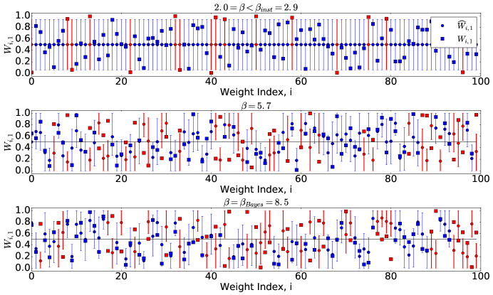
Figure 10: Bayesian credible intervals as computed by variational inference at nominal coverage level $1-\alpha=0.9$. Here $k=2$, $d=5000$, $n=2500$ and we consider three values of $\beta$: $\beta\in\{2,5.7,8.5\}$ (for reference $\beta_{\mbox{\tiny\rm inst}}\approx 2.9$, $\beta_{\mbox{\tiny\rm Bayes}}\approx 8.5$. Circles correspond to the posterior mean, and squares to the actual weights. We use red for the coordinates on which the credible interval does not cover the actual value of $w_{i,1}$.

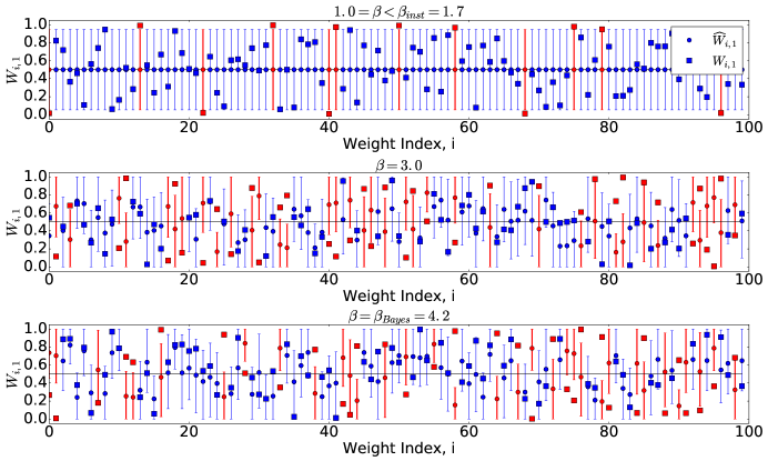
Figure 11: Bayesian credible intervals as computed by variational inference at nominal coverage level $1-\alpha=0.9$. Here $k=2$, $d=5000$, $n=10000$ and we consider three values of $\beta$: $\beta\in\{1,3,4.2\}$ (for reference $\beta_{\mbox{\tiny\rm inst}}\approx 1.7,\beta_{\mbox{\tiny\rm Bayes}}\approx 4.2$. Circles correspond to the posterior mean, and squares to the actual weights. We use red for the coordinates on which the credible interval does not cover the actual value of $w_{i,1}$.

In Figures 10 and 11 we plot Bayesian credible intervals for the weights $w_{i,1}$ as computed within naive mean field, for $k=2$, $d=5000$. These simulations are analogous to the one reported in the main text in Figure 5, but we use $n=2500$ ($\delta=0.5$) in Figure 10 and $n=10000$ ($\delta=2$) in Figure 10.

The nominal coverage of these intervals is $0.9$, but we obtain a smaller empirical coverage. For $\delta=0.5$, the empirical coverage was $0.87$ (for $\beta=2<\beta_{\mbox{\tiny\rm inst}}$), $0.61$ (for $\beta=5.7\in(\beta_{\mbox{\tiny\rm inst}},\beta_{\mbox{\tiny\rm Bayes}})$), and $0.64$ (for $\beta=8.5\approx\beta_{\mbox{\tiny\rm Bayes}}$). For $\delta=2$, the empirical coverage was $0.89$ (for $\beta=1<\beta_{\mbox{\tiny\rm inst}}$), $0.69$ (for $\beta=3\in(\beta_{\mbox{\tiny\rm inst}},\beta_{\mbox{\tiny\rm Bayes}})$), and $0.65$ (for $\beta=4.2\approx\beta_{\mbox{\tiny\rm Bayes}}$).

E.2 Results for $k=3$ topics

A

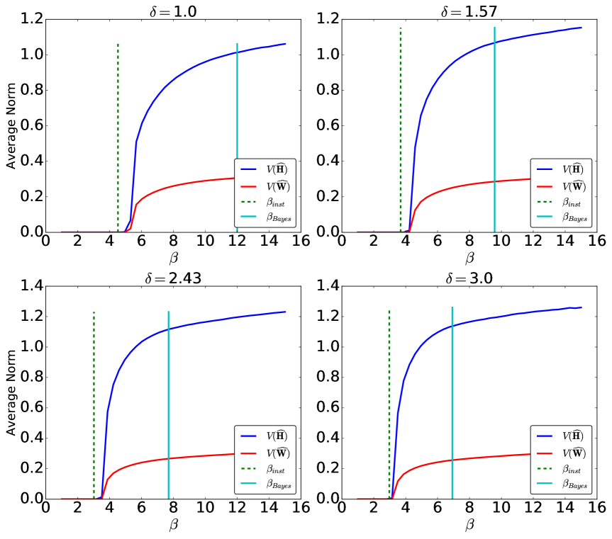
Figure 12: Normalized distances ${\sf V}({\widehat{\boldsymbol{H}}})$, ${\sf V}(\widehat{\boldsymbol{W}})$ of the naive mean field estimates from the uninformative fixed point. Here $d=1000$ and changed $n=d\delta$: each data point corresponds to an average over $400$ random realizations.

A

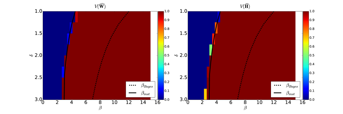
Figure 13: Empirical fraction of instances such that ${\sf V}(\widehat{\boldsymbol{W}})\geq{\varepsilon}_{0}=5\cdot 10^{-3}$ (left) or ${\sf V}({\widehat{\boldsymbol{H}}})\geq{\varepsilon}_{0}$ (right), where $\widehat{\boldsymbol{W}},{\widehat{\boldsymbol{H}}}$ are the naive mean field estimate. Here $k=3$, $d=1000$ and, for each $(\delta,\beta)$ point on a grid, we used $400$ random realizations to estimate the probability of ${\sf V}(\widehat{\boldsymbol{W}})\geq{\varepsilon}_{0}$.

A

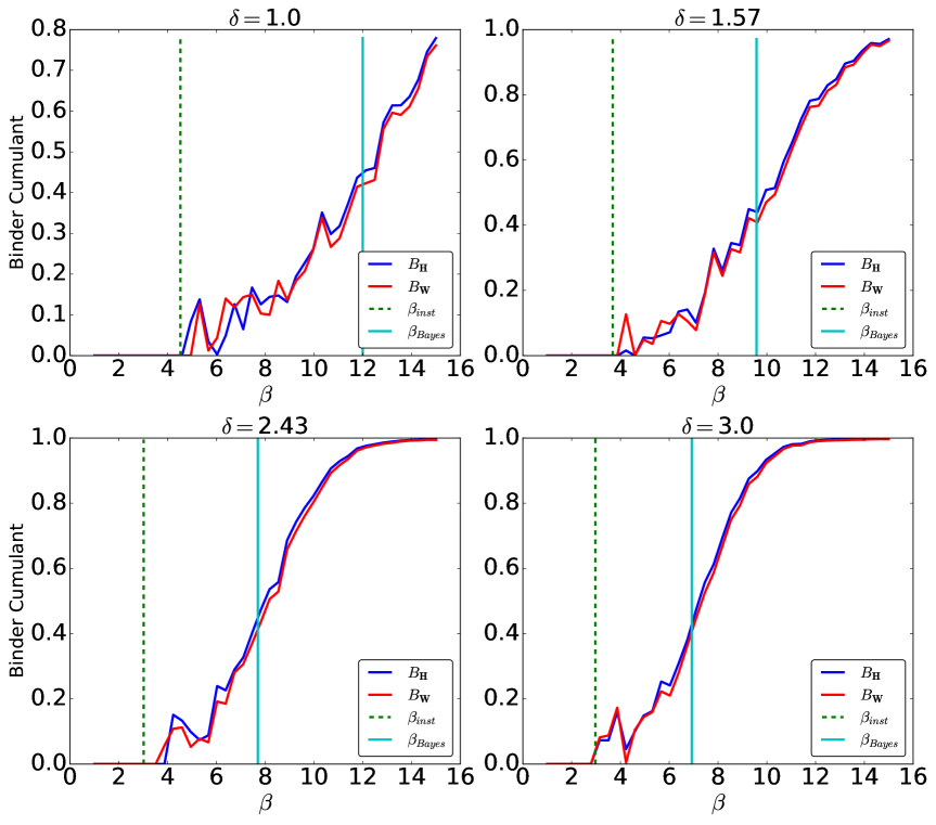
Figure 14: Binder cumulant for the correlation between the naive mean field estimates ${\widehat{\boldsymbol{H}}}$ and the true topics ${\boldsymbol{H}}$. Here we report results for $k=3$, $d=1000$ and $n=d\delta$, obtained by averaging over $400$ realizations. Note that for $\beta<\beta_{\mbox{\tiny\rm Bayes}}(k,\nu,\delta)$, ${\sf B}_{{\boldsymbol{H}}}$ decreases with the dimensions, suggesting asymptotically vanishing correlations.

A

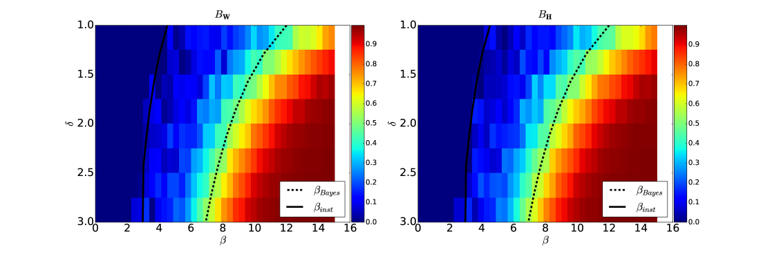
Figure 15: Binder cumulant for the correlation between the naive mean field estimates $\widehat{\boldsymbol{W}}$, ${\widehat{\boldsymbol{H}}}$ and the true weights and topics ${\boldsymbol{W}}$, ${\boldsymbol{H}}$. Here $k=3$, $d=1000$ and $n=d\delta$, and we averaged over $400$ realizations.

In Figures 12 to 15 we report our results using alternating minimization to minimize the naive mean field free energy for $k=3$.

In Figures 12, 13 we plot (respectively) the normalized distances ${\sf V}({\widehat{\boldsymbol{H}}})$, ${\sf V}(\widehat{\boldsymbol{W}})$ from the uninformative subspaces $\{{\boldsymbol{H}}={\boldsymbol{v}}\otimes{\boldsymbol{1}}_{k}:\;{\boldsymbol{v}}\in\mathbb{R}^{d}\}$ and $\{{\boldsymbol{W}}={\boldsymbol{v}}\otimes{\boldsymbol{1}}_{k}:\;{\boldsymbol{v}}\in\mathbb{R}^{d}\}$. Data are consistent with the claim that this distance becomes significant when $\beta\geq\beta_{\mbox{\tiny\rm inst}}(k,\nu,\delta)$.

In Figures 14, 15 we consider the correlation between the estimates ${\widehat{\boldsymbol{H}}},\widehat{\boldsymbol{W}}$ and the true factorization ${\boldsymbol{H}},{\boldsymbol{W}}$, and define a Binder cumulant as follows for $k\geq 3$. Let ${\sf C}_{\eta}({\boldsymbol{H}},{\widehat{\boldsymbol{H}}})$ be the $k\times k$ matrix with entries

$${\sf C}_{\eta}({\boldsymbol{H}},{\widehat{\boldsymbol{H}}})_{i,j} = \frac{\langle({\widehat{\boldsymbol{H}}}_{\perp})_{i}+\eta{\boldsymbol{g}},({\boldsymbol{H}}_{\perp})_{j}\rangle}{\|({\widehat{\boldsymbol{H}}}_{\perp})_{i}+\eta{\boldsymbol{g}}\|_{2}\|({\boldsymbol{H}}_{\perp})_{j}\|_{2}}$$ (E.1)

We then define

$$\hat{{\boldsymbol{R}}} \equiv \frac{\widehat{\mathbb{E}}\left\{\sum_{i,j\leq k}{\sf C}_{\eta}({\boldsymbol{H}},{\widehat{\boldsymbol{H}}})_{i,j}^{4}\right\}}{\widehat{\mathbb{E}}\left\{\sum_{i,j\leq k}{\sf C}_{\eta}({\boldsymbol{H}},{\widehat{\boldsymbol{H}}})_{i,j}^{2}\right\}^{2}}$$ (E.2)

$${\sf B}_{{\boldsymbol{H}}} \equiv \left\{\begin{array}[]{cl}6\bigg{(}\max\big{\{}\frac{2}{3}-\hat{{\boldsymbol{R}}}\big{\}}-\frac{1}{3}\bigg{)}&\mbox{if }\widehat{\mathbb{E}}\left\{\sum_{i,j\leq k}{\sf C}_{\eta}({\boldsymbol{H}},{\widehat{\boldsymbol{H}}})_{i,j}^{2}\right\}>0.01\,,\\ 0&\mbox{otherwise.}\end{array}\right.$$ (E.5)

Here $\widehat{\mathbb{E}}$ denotes empirical average with respect to the sample and ${\boldsymbol{g}}\sim{\sf N}(0,{\boldsymbol{I}}_{d})$. We set $\eta=10^{-4}$. An analogous definition holds for ${\sf C}_{\eta}(\widehat{\boldsymbol{W}})$, ${\sf B}_{\eta}(\widehat{\boldsymbol{W}})$. In equation (E.2) we introduced a max thresholding step and a threshold on the denominator. These are added to ensure the stability of the fraction below the phase transition region where the denominator of $\hat{\boldsymbol{R}}$ vanishes.

Figures 14, 15 are consistent with the prediction that the correlation between the AMP estimates and the true factors ${\boldsymbol{W}},{\boldsymbol{H}}$ starts to be non-negligible at the Bayes threshold.

Appendix F TAP free energy and approximate message passing

F.1 Heuristic derivation of the TAP free energy

Several heuristic approaches exist to construct the TAP free energy. Here we will derive the expression (4.3) of the TAP free energy for topic models as an approximation of the Bethe free energy for the same problem: we refer to [WJ08, MM09, KF09] for background on the latter. Let us emphasize that our derivation will be only heuristic, since our rigorous results are obtained by analyzing the resulting expression ${\cal F}_{\mbox{\tiny\rm TAP}}({\boldsymbol{r}},\tilde{\boldsymbol{r}})$ and do not require a rigorous justification of Eq. (4.3).

The posterior $p_{{\boldsymbol{H}},{\boldsymbol{W}}|\boldsymbol{X}}$ takes the form

$$p_{{\boldsymbol{H}},{\boldsymbol{W}}|\boldsymbol{X}}({\boldsymbol{H}},{\boldsymbol{W}}|\boldsymbol{X})=\frac{1}{Z(\boldsymbol{X})}\prod_{(a,i)\in[n]\times[d]}\exp\left\{\sqrt{\beta}X_{ai}\langle{\boldsymbol{w}}_{a},{\boldsymbol{h}}_{i}\rangle-\frac{\beta}{2d}\langle{\boldsymbol{w}}_{a},{\boldsymbol{h}}_{i}\rangle^{2}\right\}\prod_{a=1}^{d}\tilde{q}_{0}({\boldsymbol{w}}_{a})\prod_{i=1}^{d}q_{0}({\boldsymbol{h}}_{i})\,.$$ (F.1)

This can be regarded as a pairwise graphical model whose underlying graph is the complete bipartite graph over vertex sets $[n]$ (associated to variables ${\boldsymbol{w}}_{1}$, …${\boldsymbol{w}}_{n}$) and $[d]$ (associated to variables ${\boldsymbol{h}}_{1}$, …${\boldsymbol{h}}_{d}$). The Bethe free energy ${\cal F}_{\mbox{\tiny\rm Bethe}}$ takes as input messages $\boldsymbol{q}\equiv(q_{i\to a})_{i\in[d],a\in[n]}$, $\widetilde{\boldsymbol{q}}=(\tilde{q}_{a\to i})_{i\in[d],a\in[n]}$. Messages are probability densities over the ${\boldsymbol{h}}_{i}$’s (for $q_{i\to a}$) or the ${\boldsymbol{w}}_{a}$’s (for $\tilde{q}_{a\to i}$), indexed by the directed edges in this graph (each pair $(a,i)$, $a\in[n]$, $i\in[d]$ gives rise to two directed edges). The free energy takes the form [MM09]

$${\cal F}_{\mbox{\tiny\rm Bethe}}(\boldsymbol{q},\widetilde{\boldsymbol{q}}) =\sum_{a=1}^{n}\sum_{i=1}^{d}\log Z_{ai}-\sum_{i=1}^{d}\log Z_{i}-\sum_{a=1}^{n}\log\tilde{Z}_{a}\,,$$ (F.2)

$$Z_{i} =\int\prod_{a=1}^{n}e^{\sqrt{\beta}X_{ai}\langle{\boldsymbol{w}}_{a},{\boldsymbol{h}}_{i}\rangle-\frac{\beta}{2d}\langle{\boldsymbol{w}}_{a},{\boldsymbol{h}}_{i}\rangle^{2}}{\rm d}q_{0}({\boldsymbol{h}}_{i})\,\prod_{a=1}^{n}{\rm d}\tilde{q}_{a\to i}({\boldsymbol{w}}_{a})\,,$$ (F.3)

$$\tilde{Z}_{a} =\int\prod_{i=1}^{d}e^{\sqrt{\beta}X_{ai}\langle{\boldsymbol{w}}_{a},{\boldsymbol{h}}_{i}\rangle-\frac{\beta}{2d}\langle{\boldsymbol{w}}_{a},{\boldsymbol{h}}_{i}\rangle^{2}}{\rm d}\tilde{q}_{0}({\boldsymbol{w}}_{a})\,\prod_{i=1}^{d}{\rm d}q_{i\to a}({\boldsymbol{h}}_{i})\,,$$ (F.4)

$$Z_{ai} =\int e^{\sqrt{\beta}X_{ai}\langle{\boldsymbol{w}}_{a},{\boldsymbol{h}}_{i}\rangle-\frac{\beta}{2d}\langle{\boldsymbol{w}}_{a},{\boldsymbol{h}}_{i}\rangle^{2}}\,\,{\rm d}q_{i\to a}({\boldsymbol{h}}_{i})\,{\rm d}\tilde{q}_{a\to i}({\boldsymbol{w}}_{a})\,.$$ (F.5)

The stationarity conditions for ${\cal F}_{\mbox{\tiny\rm Bethe}}(\boldsymbol{q},\widetilde{\boldsymbol{q}})$ correspond to the belief propagation fixed point equations

$$q_{i\to b}({\boldsymbol{h}}_{i}) =\frac{1}{C_{i\to b}}\,q_{0}({\boldsymbol{h}}_{i})\,\prod_{a\in[n]\setminus b}\int e^{\sqrt{\beta}X_{ai}\langle{\boldsymbol{w}}_{a},{\boldsymbol{h}}_{i}\rangle-\frac{\beta}{2d}\langle{\boldsymbol{w}}_{a},{\boldsymbol{h}}_{i}\rangle^{2}}{\rm d}\tilde{q}_{a\to i}({\boldsymbol{w}}_{a})\,,$$ (F.6)

$$\tilde{q}_{a\to j}({\boldsymbol{w}}_{i}) =\frac{1}{\tilde{C}_{a\to j}}\,\tilde{q}_{0}({\boldsymbol{w}}_{i})\,\prod_{i\in[d]\setminus j}\int e^{\sqrt{\beta}X_{ai}\langle{\boldsymbol{w}}_{a},{\boldsymbol{h}}_{i}\rangle-\frac{\beta}{2d}\langle{\boldsymbol{w}}_{a},{\boldsymbol{h}}_{i}\rangle^{2}}{\rm d}q_{i\to a}({\boldsymbol{h}}_{i})\,.$$ (F.7)

We define ${\boldsymbol{f}}_{i\to a}=\int{\boldsymbol{h}}_{i}{\rm d}q_{i\to a}({\boldsymbol{h}}_{i})$, $\tilde{\boldsymbol{f}}_{a\to i}=\int{\boldsymbol{w}}_{a}{\rm d}\tilde{q}_{a\to i}({\boldsymbol{w}}_{a})$, and ${\boldsymbol{g}}_{i\to a}=\int{\boldsymbol{h}}^{\otimes 2}_{i}{\rm d}q_{i\to a}({\boldsymbol{h}}_{i})$, $\tilde{\boldsymbol{g}}_{a\to i}=\int{\boldsymbol{w}}^{\otimes 2}_{a}{\rm d}\tilde{q}_{a\to i}({\boldsymbol{w}}_{a})$. Since $X_{ai}=O(1/\sqrt{n})$, we have

$$\prod_{i=1}^{d} \int e^{\sqrt{\beta}X_{ai}\langle{\boldsymbol{w}}_{a},{\boldsymbol{h}}_{i}\rangle-\frac{\beta}{2d}\langle{\boldsymbol{w}}_{a},{\boldsymbol{h}}_{i}\rangle^{2}}{\rm d}q_{i\to a}({\boldsymbol{h}}_{i})=$$ (F.8)

$$=\prod_{i=1}^{d}\exp\left\{\sqrt{\beta}X_{ai}\langle{\boldsymbol{f}}_{i\to a},{\boldsymbol{w}}_{a}\rangle-\frac{\beta}{2d}\langle{\boldsymbol{f}}_{i\to a},{\boldsymbol{w}}_{a}\rangle^{2}+\frac{\beta}{2}\Big{(}X_{ai}^{2}-\frac{1}{d}\Big{)}\langle{\boldsymbol{g}}_{i\to a}-{\boldsymbol{f}}_{i\to a}^{\otimes 2},{\boldsymbol{w}}_{a}^{\otimes 2}\rangle+O(n^{-3/2})\right\}$$ (F.9)

$$=\exp\left\{\sum_{i=1}^{d}\sqrt{\beta}X_{ai}\langle{\boldsymbol{f}}_{i\to a},{\boldsymbol{w}}_{a}\rangle-\frac{\beta}{2d}\sum_{i=1}^{d}\langle{\boldsymbol{f}}_{i\to a},{\boldsymbol{w}}_{a}\rangle^{2}+O(n^{-1/2})\right\}\,,$$ (F.10)

where in the last step we used the fact that ${\mathbb{E}}\{X^{2}_{ai}-d^{-1}\}=O(n^{-3/2})$ and applied the central limit theorem.

Using the expression (F.10) in Eq. (F.4), and repeating a similar calculation for (F.3), we get

$$\log Z_{i} =\phi\left(\sqrt{\beta}\sum_{a=1}^{n}X_{ai}\tilde{\boldsymbol{f}}_{a\to i},\frac{\beta}{d}\sum_{a=1}^{n}\tilde{\boldsymbol{f}}_{a\to i}^{\otimes 2}\right)+O(n^{-1/2})\,,$$ (F.11)

$$\log\tilde{Z}_{a} ={\tilde{\phi}}\left(\sqrt{\beta}\sum_{i=1}^{d}X_{ai}{\boldsymbol{f}}_{i\to a},\frac{\beta}{d}\sum_{i=1}^{d}{\boldsymbol{f}}_{i\to a}^{\otimes 2}\right)+O(n^{-1/2})\,,$$ (F.12)

where the functions $\phi$, ${\tilde{\phi}}$ are defined implicitly in Eq. (3.5).

We can similarly expand $Z_{ai}$ for large $n,d$:

$$Z_{ai} =1+\sqrt{\beta}X_{ai}\langle\tilde{\boldsymbol{f}}_{a\to i},{\boldsymbol{f}}_{i\to a}\rangle+\frac{\beta}{2}\Big{(}X_{ai}^{2}-\frac{1}{d}\Big{)}\langle\tilde{\boldsymbol{g}}_{a\to i},{\boldsymbol{g}}_{i\to a}\rangle+O(n^{-3/2})$$ (F.13)

$$=\exp\left\{\sqrt{\beta}X_{ai}\langle\tilde{\boldsymbol{f}}_{a\to i},{\boldsymbol{f}}_{i\to a}\rangle-\frac{\beta}{2}X_{ai}^{2}\langle\tilde{\boldsymbol{f}}_{a\to i},{\boldsymbol{f}}_{i\to a}\rangle^{2}+\frac{\beta}{2}\Big{(}X_{ai}^{2}-\frac{1}{d}\Big{)}\langle\tilde{\boldsymbol{g}}_{a\to i},{\boldsymbol{g}}_{i\to a}\rangle+O(n^{-3/2})\right\}\,.$$ (F.14)

Therefore, using again the central limit theorem,

$$\sum_{a\leq n,i\leq d}\log Z_{ai} =\sqrt{\beta}\sum_{a\leq n,i\leq d}X_{ai}\langle\tilde{\boldsymbol{f}}_{a\to i},{\boldsymbol{f}}_{i\to a}\rangle-\frac{\beta}{2d}\sum_{a\leq n,i\leq d}\langle\tilde{\boldsymbol{f}}_{a\to i},{\boldsymbol{f}}_{i\to a}\rangle^{2}+O(n^{1/2})\,.$$ (F.15)

Putting together Eqs. (F.11), (F.12), and (F.15), we obtain

$${\cal F}_{\mbox{\tiny\rm Bethe}}(\boldsymbol{q},\widetilde{\boldsymbol{q}}) =-\sum_{i=1}^{d}\phi\left(\sqrt{\beta}\sum_{a=1}^{n}X_{ai}\tilde{\boldsymbol{f}}_{a\to i},\frac{\beta}{d}\sum_{a=1}^{n}\tilde{\boldsymbol{f}}_{a\to i}^{\otimes 2}\right)-\sum_{a=1}^{n}{\tilde{\phi}}\left(\sqrt{\beta}\sum_{i=1}^{d}X_{ai}{\boldsymbol{f}}_{i\to a},\frac{\beta}{d}\sum_{i=1}^{d}{\boldsymbol{f}}_{i\to a}^{\otimes 2}\right)$$

$$+\sqrt{\beta}\sum_{a\leq n,i\leq d}X_{ai}\langle\tilde{\boldsymbol{f}}_{a\to i},{\boldsymbol{f}}_{i\to a}\rangle-\frac{\beta}{2d}\sum_{a\leq n,i\leq d}\langle\tilde{\boldsymbol{f}}_{a\to i},{\boldsymbol{f}}_{i\to a}\rangle^{2}+O(n^{1/2})\,.$$ (F.16)

Close to the solution of the stationarity conditions (F.6), (F.7), the message ${\boldsymbol{f}}_{i\to a}$ should be roughly independent of $a\in[n]$ and $\tilde{\boldsymbol{f}}_{a\to i}$ should be roughly independent of $i\in[d]$. Hence, we can approximate

$$-\frac{\beta}{2d}\sum_{a\leq n,i\leq d}\langle\tilde{\boldsymbol{f}}_{a\to i},{\boldsymbol{f}}_{i\to a}\rangle^{2}=-\frac{\beta}{2nd^{2}}\sum_{a\leq n,i\leq d}\sum_{b\leq n,j\leq d}\langle\tilde{\boldsymbol{f}}_{a\to j},{\boldsymbol{f}}_{i\to b}\rangle^{2}+o(n)\,.$$ (F.17)

In order to obtain the expression of Eq. (4.3) we add auxiliary variables ${\boldsymbol{m}}_{i},\tilde{\boldsymbol{m}}_{a}\in\mathbb{R}^{k}$, and ${\boldsymbol{Q}}_{i},\widetilde{\boldsymbol{Q}}_{a}\in\mathbb{R}^{k\times k}$, alongside Lagrange multipliers ${\boldsymbol{r}}_{i}$, $\tilde{\boldsymbol{r}}_{a}$, ${\boldsymbol{\Omega}}_{i}$, $\tilde{\boldsymbol{\Omega}}_{a}$ to enforce the constraints

$${\boldsymbol{m}}_{i}=\sqrt{\beta}\sum_{a=1}^{n}X_{ai}\tilde{\boldsymbol{f}}_{a\to i}\,,\;\;\;\;\;\;\;{\boldsymbol{Q}}_{i}=\frac{\beta}{d}\sum_{a=1}^{n}\tilde{\boldsymbol{f}}_{a\to i}^{\otimes 2}\,,$$ (F.18)

$${\boldsymbol{m}}_{a}=\sqrt{\beta}\sum_{i=1}^{d}X_{ai}{\boldsymbol{f}}_{i\to a}\,,\;\;\;\;\;\;\;\widetilde{\boldsymbol{Q}}_{a}=\frac{\beta}{d}\sum_{i=1}^{d}{\boldsymbol{f}}_{i\to a}^{\otimes 2}\,.$$ (F.19)

Denoting by ${\boldsymbol{m}}\in\mathbb{R}^{d\times k}$ the matrix whose $i$-th row is ${\boldsymbol{m}}_{i}$ (and analogously for $\tilde{\boldsymbol{m}}$, ${\boldsymbol{f}}$, $\tilde{\boldsymbol{f}}$ and the Lagrange multipliers ${\boldsymbol{r}}$, $\tilde{\boldsymbol{r}}$), and using Eq. (F.17) we obtain the Lagrangian (here all sums run over $a\in[n]$ and $i\in[d]$)

$${\mathcal{L}}= \langle{\boldsymbol{r}},{\boldsymbol{m}}\rangle-\sqrt{\beta}\sum_{a,i}X_{ai}\langle{\boldsymbol{r}}_{i},\tilde{\boldsymbol{f}}_{a\to i}\rangle+\langle\tilde{\boldsymbol{r}},\tilde{\boldsymbol{m}}\rangle-\sqrt{\beta}\sum_{a,i}X_{ai}\langle\tilde{\boldsymbol{r}}_{a},{\boldsymbol{f}}_{i\to a}\rangle+\sqrt{\beta}\sum_{a,i}X_{ai}\langle\tilde{\boldsymbol{f}}_{a\to i},{\boldsymbol{f}}_{i\to a}\rangle$$

$$+\frac{\sqrt{\beta}}{2n}\sum_{a,i}\langle\tilde{\boldsymbol{\Omega}}_{a},{\boldsymbol{f}}_{i\to a}^{\otimes 2}\rangle-\frac{d}{2n\sqrt{\beta}}\sum_{a}\langle\tilde{\boldsymbol{\Omega}}_{a},\widetilde{\boldsymbol{Q}}_{a}\rangle+\frac{\sqrt{\beta}}{2d}\sum_{a,i}\langle\tilde{\boldsymbol{\Omega}}_{i},\tilde{\boldsymbol{f}}_{a\to i}^{\otimes 2}\rangle-\frac{d}{2d\sqrt{\beta}}\sum_{a}\langle{\boldsymbol{\Omega}}_{i},\widetilde{\boldsymbol{Q}}_{i}\rangle$$

$$-\sum_{i}\phi({\boldsymbol{m}}_{i},{\boldsymbol{Q}}_{i})-\sum_{a}{\tilde{\phi}}(\tilde{\boldsymbol{m}}_{i},\widetilde{\boldsymbol{Q}}_{i})-\frac{d}{2\beta dn}\sum_{a,i}\langle\widetilde{\boldsymbol{Q}}_{a},{\boldsymbol{Q}}_{i}\rangle\,.$$ (F.20)

We next minimize with respect to the message variables $({\boldsymbol{f}}_{i\to a})$, $(\tilde{\boldsymbol{f}}_{a\to i})$. The first order stationarity conditions read

$$X_{ai}\tilde{\boldsymbol{f}}_{a\to i} =X_{ai}\tilde{\boldsymbol{r}}_{a}-\frac{1}{n}\tilde{\boldsymbol{\Omega}}_{a}{\boldsymbol{f}}_{i\to a}\,,$$ (F.21)

$$X_{ai}{\boldsymbol{f}}_{i\to a} =X_{ai}{\boldsymbol{r}}_{i}-\frac{1}{d}{\boldsymbol{\Omega}}_{i}\tilde{\boldsymbol{f}}_{a\to i}\,.$$ (F.22)

In particular these imply that $\tilde{\boldsymbol{f}}_{a\to i}=\tilde{\boldsymbol{r}}_{a}+O(1/\sqrt{n})$ and $\tilde{\boldsymbol{f}}_{a\to i}=\tilde{\boldsymbol{r}}_{a}+O(1/\sqrt{n})$. Multiplying the first of these equations by ${\boldsymbol{f}}_{i\to a}$ and the second by $\tilde{\boldsymbol{f}}_{a\to i}$, and summing over $i,a$ we obtain

$$\sum_{a,i}X_{ai}\langle\tilde{\boldsymbol{f}}_{a\to i},{\boldsymbol{f}}_{i\to a}\rangle= \frac{1}{2}\sum_{i,a}X_{ai}\Big{(}\langle{\boldsymbol{f}}_{i\to a},\tilde{\boldsymbol{r}}_{a}\rangle+\langle\tilde{\boldsymbol{f}}_{a\to i},{\boldsymbol{r}}_{i}\rangle\Big{)}-\frac{1}{2n}\sum_{i,a}\langle\tilde{\boldsymbol{\Omega}}_{a},{\boldsymbol{f}}_{i\to a}^{\otimes 2}\rangle-\frac{1}{2d}\sum_{i,a}\langle{\boldsymbol{\Omega}}_{i},\tilde{\boldsymbol{f}}_{a\to i}^{\otimes 2}\rangle$$

$$= \frac{1}{2}\sum_{i,a}X_{ai}\Big{(}\langle{\boldsymbol{f}}_{i\to a},\tilde{\boldsymbol{r}}_{a}\rangle+\langle\tilde{\boldsymbol{f}}_{a\to i},{\boldsymbol{r}}_{i}\rangle\Big{)}-\frac{1}{2n}\sum_{i,a}\langle\tilde{\boldsymbol{\Omega}}_{a},{\boldsymbol{r}}_{i}^{\otimes 2}\rangle-\frac{1}{2d}\sum_{i,a}\langle{\boldsymbol{\Omega}}_{i},\tilde{\boldsymbol{r}}_{a}^{\otimes 2}\rangle+O(n^{1/2})\,.$$ (F.23)

Further, multiplying Eqs. (F.21), (F.22) respectively by ${\boldsymbol{r}}_{i}$ and $\tilde{\boldsymbol{r}}_{a}$, we get

$$\frac{1}{2}\sum_{i,a}X_{ai}\Big{(}\langle{\boldsymbol{f}}_{i\to a},\tilde{\boldsymbol{r}}_{a}\rangle +\langle\tilde{\boldsymbol{f}}_{a\to i},{\boldsymbol{r}}_{i}\rangle\Big{)}=\sum_{a,i}X_{ai}\langle\tilde{\boldsymbol{r}}_{a},{\boldsymbol{r}}_{i}\rangle-\frac{1}{2n}\sum_{a,i}\langle{\boldsymbol{r}}_{i},\tilde{\boldsymbol{\Omega}}_{a}{\boldsymbol{f}}_{i\to a}\rangle-\frac{1}{2d}\sum_{a,i}\langle\tilde{\boldsymbol{r}}_{a},{\boldsymbol{\Omega}}_{i}\tilde{\boldsymbol{f}}_{a\to i}\rangle$$

$$=\sum_{a,i}X_{ai}\langle\tilde{\boldsymbol{r}}_{a},{\boldsymbol{r}}_{i}\rangle-\frac{1}{2n}\sum_{a,i}\langle\tilde{\boldsymbol{\Omega}}_{a},{\boldsymbol{r}}_{i}^{\otimes 2}\rangle-\frac{1}{2d}\sum_{a,i}\langle{\boldsymbol{\Omega}}_{i},\tilde{\boldsymbol{r}}_{a}^{\otimes 2}\rangle+O(n^{1/2})\,.$$ (F.24)

Substituting the last two expressions in Eq. (F.20), we obtain

$${\mathcal{L}}= \;\langle{\boldsymbol{r}},{\boldsymbol{m}}\rangle+\langle\tilde{\boldsymbol{r}},\tilde{\boldsymbol{m}}\rangle-\sqrt{\beta}\langle\tilde{\boldsymbol{r}},\boldsymbol{X}{\boldsymbol{r}}\rangle+\frac{\sqrt{\beta}}{2n}\sum_{a,i}\langle\tilde{\boldsymbol{\Omega}}_{a},{\boldsymbol{r}}_{i}^{\otimes 2}\rangle+\frac{\sqrt{\beta}}{2d}\sum_{a,i}\langle{\boldsymbol{\Omega}}_{i},\tilde{\boldsymbol{r}}_{a}^{\otimes 2}\rangle-\frac{d}{2n\sqrt{\beta}}\sum_{a}\langle\tilde{\boldsymbol{\Omega}}_{a},\widetilde{\boldsymbol{Q}}_{a}\rangle$$

$$-\frac{d}{2d\sqrt{\beta}}\sum_{i}\langle{\boldsymbol{\Omega}}_{i},{\boldsymbol{Q}}_{i}\rangle-\sum_{i}\phi({\boldsymbol{m}}_{i},{\boldsymbol{Q}}_{i})-\sum_{a}{\tilde{\phi}}(\tilde{\boldsymbol{m}}_{i},\widetilde{\boldsymbol{Q}}_{i})-\frac{d}{2\beta dn}\sum_{a,i}\langle\widetilde{\boldsymbol{Q}}_{a},{\boldsymbol{Q}}_{i}\rangle+O(n^{1/2})\,.$$ (F.25)

Setting ${\boldsymbol{Q}}_{i}={\boldsymbol{Q}}$ independent of $i$, $\widetilde{\boldsymbol{Q}}_{a}=\widetilde{\boldsymbol{Q}}$ independent of $a$, defining ${\boldsymbol{\Omega}}=d^{-1}\sum_{i=1}^{d}{\boldsymbol{\Omega}}_{i}$, $\tilde{\boldsymbol{\Omega}}=n^{-1}\sum_{a=1}^{n}\tilde{\boldsymbol{\Omega}}_{a}$, and neglecting $o(n)$ terms, we get

$$\begin{split}\tilde{{\cal F}}_{\mbox{\tiny\rm TAP}}=&\frac{d}{2}\|\boldsymbol{X}\|_{F}-\sqrt{\beta}{\sf{Tr}}\left(\boldsymbol{X}{\boldsymbol{r}}\tilde{\boldsymbol{r}}^{{\sf T}}\right)+{\sf{Tr}}({\boldsymbol{r}}^{{\sf T}}{\boldsymbol{m}})+{\sf{Tr}}(\tilde{\boldsymbol{r}}^{{\sf T}}\tilde{\boldsymbol{m}})-\frac{d}{2\sqrt{\beta}}{\sf{Tr}}({\boldsymbol{Q}}{\boldsymbol{\Omega}})-\frac{d}{2\sqrt{\beta}}{\sf{Tr}}(\widetilde{\boldsymbol{Q}}\tilde{\boldsymbol{\Omega}})\\ &-\sum_{a=1}^{n}{\tilde{\phi}}(\tilde{\boldsymbol{m}}_{a},\widetilde{\boldsymbol{Q}})-\sum_{i=1}^{d}\phi({\boldsymbol{m}}_{i},{\boldsymbol{Q}})+\frac{\sqrt{\beta}}{2}\sum_{i=1}^{d}\langle\tilde{\boldsymbol{\Omega}},{\boldsymbol{r}}_{i}^{\otimes 2}\rangle+\frac{\sqrt{\beta}}{2}\sum_{a=1}^{n}\langle{\boldsymbol{\Omega}},\tilde{\boldsymbol{r}}_{a}^{\otimes 2}\rangle\\ &-\frac{d}{2\beta}\langle{\boldsymbol{Q}},\widetilde{\boldsymbol{Q}}\rangle\,.\end{split}$$ (F.26)

Finally, the expression (4.3) is recovered by using the stationarity conditions with respect to ${\boldsymbol{\Omega}}$ and $\tilde{\boldsymbol{\Omega}}$, which imply ${\boldsymbol{Q}}=(\sqrt{\beta}/d)\sum_{a=1}^{n}\tilde{\boldsymbol{r}}_{a}^{\otimes 2}$ and $\widetilde{\boldsymbol{Q}}=(\sqrt{\beta}/d)\sum_{i=1}^{d}{\boldsymbol{r}}_{i}^{\otimes 2}$, and maximizing with respect to ${\boldsymbol{m}}$, $\tilde{\boldsymbol{m}}$.

F.2 Gradient of the TAP free energy

From the definition of the partial Legendre transforms $\psi({\boldsymbol{r}},{\boldsymbol{Q}})$, ${\tilde{\psi}}(\tilde{\boldsymbol{r}},\widetilde{\boldsymbol{Q}})$, the following derivatives hold

$$\frac{\partial\psi}{\partial{\boldsymbol{r}}}({\boldsymbol{r}},{\boldsymbol{Q}})={\boldsymbol{m}}({\boldsymbol{r}},{\boldsymbol{Q}})\,,\;\;\;\;\;\;\;\frac{\partial\psi}{\partial{\boldsymbol{Q}}}({\boldsymbol{r}},{\boldsymbol{Q}})=-\frac{1}{2\beta}{\sf G}\big{(}{\boldsymbol{m}}({\boldsymbol{r}},{\boldsymbol{Q}}),{\boldsymbol{Q}}\big{)}\,,$$ (F.27)

where ${\boldsymbol{m}}({\boldsymbol{r}},{\boldsymbol{Q}})\in\mathbb{R}^{k}$ is the unique solution of

$${\boldsymbol{r}}=\frac{1}{\sqrt{\beta}}\,{\sf F}({\boldsymbol{m}};{\boldsymbol{Q}})\,.$$ (F.28)

Using these derivatives we can compute the gradient of the free energy

$$\frac{\partial{\cal F}_{\mbox{\tiny\rm TAP}}}{\partial{\boldsymbol{r}}_{i}}({\boldsymbol{r}},\tilde{\boldsymbol{r}}) =-\sqrt{\beta}(\boldsymbol{X}^{{\sf T}}\tilde{\boldsymbol{r}})_{i}+{\boldsymbol{m}}_{i}-\frac{\beta}{d}\sum_{a=1}^{n}\langle\tilde{\boldsymbol{r}}_{a},{\boldsymbol{r}}_{i}\rangle\,\tilde{\boldsymbol{r}}_{a}+\frac{1}{d}\sum_{a=1}^{n}\widetilde{\sf G}(\tilde{\boldsymbol{m}}_{a},\widetilde{\boldsymbol{Q}}){\boldsymbol{r}}_{i}$$

$$=-\sqrt{\beta}(\boldsymbol{X}^{{\sf T}}\tilde{\boldsymbol{r}})_{i}+{\boldsymbol{m}}_{i}+\sqrt{\beta}\tilde{\boldsymbol{\Omega}}{\boldsymbol{r}}_{i}\,,$$ (F.29)

$$\frac{\partial{\cal F}_{\mbox{\tiny\rm TAP}}}{\partial\tilde{\boldsymbol{r}}_{a}}({\boldsymbol{r}},\tilde{\boldsymbol{r}}) =-\sqrt{\beta}(\boldsymbol{X}{\boldsymbol{r}})_{a}+\tilde{\boldsymbol{m}}_{a}-\frac{\beta}{d}\sum_{i=1}^{d}\langle\tilde{\boldsymbol{r}}_{a},{\boldsymbol{r}}_{i}\rangle\,{\boldsymbol{r}}_{i}+\frac{1}{d}\sum_{i=1}^{d}{\sf G}({\boldsymbol{m}}_{i},{\boldsymbol{Q}})\tilde{\boldsymbol{r}}_{a}$$

$$=-\sqrt{\beta}(\boldsymbol{X}{\boldsymbol{r}})_{a}+\tilde{\boldsymbol{m}}_{a}+\sqrt{\beta}{\boldsymbol{\Omega}}\tilde{\boldsymbol{r}}_{a}\,,$$ (F.30)

where ${\boldsymbol{m}}_{i}={\boldsymbol{m}}({\boldsymbol{r}}_{i},(\beta/d)\sum_{a\leq n}\tilde{\boldsymbol{r}}_{a}^{\otimes 2})$, $\tilde{\boldsymbol{m}}_{a}=\tilde{\boldsymbol{m}}(\tilde{\boldsymbol{r}}_{a},(\beta/d)\sum_{i\leq d}{\boldsymbol{r}}_{i}^{\otimes 2})$, are defined as above, ${\boldsymbol{Q}}=(\beta/d)\sum_{a\leq n}\tilde{\boldsymbol{r}}_{a}^{\otimes 2}$, ${\boldsymbol{Q}}=(\beta/d)\sum_{i\leq d}\tilde{\boldsymbol{r}}_{i}^{\otimes 2}$, and

$${\boldsymbol{\Omega}} =\frac{1}{d\sqrt{\beta}}\sum_{i=1}^{d}\big{\{}{\sf G}({\boldsymbol{m}}_{i},{\boldsymbol{Q}})-{\sf F}({\boldsymbol{m}}_{i},{\boldsymbol{Q}})^{\otimes 2}\big{\}}\,,$$ (F.31)

$$\tilde{\boldsymbol{\Omega}} =\frac{1}{d\sqrt{\beta}}\sum_{a=1}^{n}\big{\{}\widetilde{\sf G}(\tilde{\boldsymbol{m}}_{a},\widetilde{\boldsymbol{Q}})-\widetilde{\sf F}({\boldsymbol{m}}_{a},\widetilde{\boldsymbol{Q}})^{\otimes 2}\big{\}}\,.$$ (F.32)

Remark F.1.

We can express ${\boldsymbol{r}}$, $\tilde{\boldsymbol{r}}$ in terms of ${\boldsymbol{m}}$, $\tilde{\boldsymbol{m}}$ in Eqs. (F.29), (F.30) by using Eq. (F.28)

$${\boldsymbol{m}} =\boldsymbol{X}^{{\sf T}}\,\widetilde{\sf F}(\tilde{\boldsymbol{m}};\widetilde{\boldsymbol{Q}})-{\sf F}({\boldsymbol{m}};{\boldsymbol{Q}})\tilde{\boldsymbol{\Omega}}\,,\;\;\;\;\;\;\tilde{\boldsymbol{m}}=\boldsymbol{X}\,{\sf F}({\boldsymbol{m}};{\boldsymbol{Q}})-\widetilde{\sf F}(\tilde{\boldsymbol{m}};\widetilde{\boldsymbol{Q}}){\boldsymbol{\Omega}}\,,$$ (F.33)

$${\boldsymbol{Q}} =\frac{1}{d}\sum_{a=1}^{n}\widetilde{\sf F}(\tilde{\boldsymbol{m}}_{a};\widetilde{\boldsymbol{Q}})^{\otimes 2}\,,\;\;\;\;\;\;\;\;\;\;\;\widetilde{\boldsymbol{Q}}=\frac{1}{d}\sum_{i=1}^{d}{\sf F}({\boldsymbol{m}}_{i};{\boldsymbol{Q}})^{\otimes 2}\,.$$ (F.34)

These coincide with the fixed point of the AMP algorithm in Section 4.2.

F.3 Uninformative critical point: Proof of Lemma 4.1

Consider the stationarity conditions (F.33) and (F.34), together with the definitions of Eqs. (4.10), (4.11). Since these are invariant under permutations of the topics, they admit a solution of the form ${\boldsymbol{m}}={\boldsymbol{v}}{\boldsymbol{1}}^{{\sf T}}_{k}$, $\tilde{\boldsymbol{m}}=\tilde{\boldsymbol{v}}{\boldsymbol{1}}^{{\sf T}}_{k}$, ${\boldsymbol{Q}}=q_{0}{\boldsymbol{J}}_{k}+q_{0}^{\prime}{\boldsymbol{I}}_{k}$, $\widetilde{\boldsymbol{Q}}=\tilde{q}_{0}{\boldsymbol{J}}_{k}+\tilde{q}_{0}^{\prime}{\boldsymbol{I}}_{k}$. Using Eq. (F.34) and Lemma D.1, Eqs. (D.56), (D.58), we get $q_{0}^{\prime}=\tilde{q}^{\prime}_{0}=0$.

Substituting this in Eqs. (4.10), (4.11), and using again Lemma D.1, we get

$${\boldsymbol{\Omega}}=\sqrt{\beta}\,{\boldsymbol{I}}_{k}\,,\;\;\;\;\;\;\;\;\tilde{\boldsymbol{\Omega}}=\frac{\sqrt{\beta}\delta}{k(k\nu+1)}{\boldsymbol{P}}_{\perp}\,,$$ (F.35)

where we recall that ${\boldsymbol{P}}_{\perp}={\boldsymbol{I}}_{k}-{\boldsymbol{1}}_{k}{\boldsymbol{1}}_{k}/k$. Substituting these in Eq. (F.33), we obtained that this is satisfied provided ${\boldsymbol{v}},\tilde{\boldsymbol{v}}$ are given as in Eqs. (4.12), (4.13). Finally, $q_{0}$, $\tilde{q}_{0}$ are fixed by substituting in Eq. (F.34).

Appendix G State evolution analysis

G.1 State evolution equations

Note that there is an alternative way to express the state evolution recursion in Eqs. (4.16), (4.17). Given a probability measure $p$ on $\mathbb{R}^{k}$ and a matrix ${\boldsymbol{M}}\succeq 0$, ${\boldsymbol{M}}\in\mathbb{R}^{k\times k}$, we define the minimum mean square error

$${\sf mmse}({\boldsymbol{M}};p)\equiv\inf_{\hat{\boldsymbol{x}}(\,\cdot\,)}\,{\mathbb{E}}\Big{\{}[{\boldsymbol{x}}-\hat{\boldsymbol{x}}({\boldsymbol{y}})][{\boldsymbol{x}}-\hat{\boldsymbol{x}}({\boldsymbol{y}})]^{{\sf T}}\Big{\}}\,,$$ (G.1)

where the expectation is with respect to ${\boldsymbol{x}}\sim p(\,\cdot\,)$ and ${\boldsymbol{y}}={\boldsymbol{M}}^{1/2}{\boldsymbol{x}}+{\boldsymbol{z}}$ for ${\boldsymbol{z}}\sim{\sf N}(0,{\boldsymbol{I}}_{k})$. The infimum is understood in the positive semidefinite order, and it is achieved by $\hat{\boldsymbol{x}}({\boldsymbol{y}})={\mathbb{E}}\{{\boldsymbol{x}}|{\boldsymbol{y}}\}$. We then rewrite Eqs. (4.16), (4.17) as

$${\boldsymbol{M}}_{t+1} =\beta\delta\,\Big{\{}{\sf mmse}(0;\tilde{q}_{0})-{\sf mmse}(\widetilde{\boldsymbol{M}}_{t};\tilde{q}_{0})\Big{\}}\,,$$ (G.2)

$$\widetilde{\boldsymbol{M}}_{t} =\beta\,\Big{\{}{\sf mmse}(0;q_{0})-{\sf mmse}({\boldsymbol{M}}_{t};q_{0})\Big{\}}\,.$$ (G.3)

G.2 Uninformative fixed point

Lemma G.1.

The state evolution recursion in (4.16), (4.17) admit uninformative fixed point of the form

$$\begin{split}&\widetilde{\boldsymbol{M}}^{*}=\rho_{0}{\boldsymbol{J}}_{k},\quad\quad\rho_{0}=\frac{\delta\beta^{2}}{k\delta\beta+k^{2}},\\ &{\boldsymbol{M}}^{*}=\frac{\delta\beta}{k^{2}}{\boldsymbol{J}}_{k}.\end{split}$$ (G.4)

Proof.

First note that for this value of $\widetilde{\boldsymbol{M}}^{*}$, $\widetilde{\boldsymbol{M}}^{*}{\boldsymbol{w}}+\widetilde{\boldsymbol{M}}^{*^{1/2}}{\boldsymbol{z}}=y{\boldsymbol{1}}_{k}$ for some (random) $y$. Hence, using Eq. (D.58)

$$\delta\,{\mathbb{E}}\Big{\{}\widetilde{\sf F}(\widetilde{\boldsymbol{M}}^{*}{\boldsymbol{w}}+\widetilde{\boldsymbol{M}}^{*^{1/2}}{\boldsymbol{z}};\widetilde{\boldsymbol{M}}^{*})^{\otimes 2}\Big{\}}=\frac{\delta\beta}{k^{2}}{\boldsymbol{J}}_{k}={\boldsymbol{M}}^{*}.$$ (G.5)

In addition, using the explicit form (D.5)

$${\mathbb{E}}\Big{\{}{\sf F}({\boldsymbol{M}}^{*}{\boldsymbol{h}}+{\boldsymbol{M}}^{*^{1/2}}{\boldsymbol{z}};{\boldsymbol{M}}^{*})^{\otimes 2}\Big{\}}=\beta({\boldsymbol{I}}_{k}+{\boldsymbol{M}}^{*})^{-1}{\boldsymbol{M}}^{*}=\frac{\beta^{2}\delta}{k^{2}}\left({\boldsymbol{I}}_{k}+\frac{\delta\beta}{k^{2}}{\boldsymbol{J}}_{k}\right)^{-1}{\boldsymbol{J}}_{k}=\rho_{0}{\boldsymbol{J}}_{k}=\widetilde{\boldsymbol{M}}^{*}.$$ (G.6)

Hence, the pair ${\boldsymbol{M}}^{*},\widetilde{\boldsymbol{M}}^{*}$ in (G.4) is a fixed point for the iterations in (4.16), (4.17). ∎

G.3 Stability of state evolution and proof of Theorem 4

The following theorem characterizes the region of parameters in which the uninformative fixed point of the state evolution iterations in Lemma G.1 is stable.

Theorem 6.

Consider the state evolution equations in (4.16), (4.17). The uninformative symmetric fixed point of these equations is stable if and only if

$$\beta<\beta_{\mbox{\tiny\rm spect}}=\frac{k(k\nu+1)}{\sqrt{\delta}}.$$ (G.7)

Proof.

We linearize Eqs. (4.16), (4.17) around the fixed point in (G.4) by setting ${\boldsymbol{M}}_{t}={\boldsymbol{M}}_{*}+{\boldsymbol{\Delta}}_{t}$, $\widetilde{\boldsymbol{M}}_{t}=\widetilde{\boldsymbol{M}}_{*}+\widetilde{\boldsymbol{\Delta}}_{t}$ and expanding Eqs. (4.16), (4.17) to first order in ${\boldsymbol{\Delta}},\widetilde{\boldsymbol{\Delta}}_{t}$. First note that Eq. (4.17) takes the explicit form

$$\widetilde{\boldsymbol{M}}_{t}=\beta({\boldsymbol{I}}_{k}+{\boldsymbol{M}}_{t})^{-1}{\boldsymbol{M}}_{t}\,.$$ (G.8)

Hence, expanding to linear order we get

$$\widetilde{\boldsymbol{\Delta}}_{t}=\beta\left({\boldsymbol{I}}_{k}+\frac{\delta\beta}{k^{2}}{\boldsymbol{J}}_{k}\right)^{-1}{\boldsymbol{\Delta}}_{t}\left({\boldsymbol{I}}_{k}+\frac{\delta\beta}{k^{2}}{\boldsymbol{J}}_{k}\right)^{-1}+o({\boldsymbol{\Delta}}_{t})\,.$$ (G.9)

In the following, we shall decompose ${\boldsymbol{\Delta}}_{t}$ and $\widetilde{\boldsymbol{\Delta}}_{t}$ in the components along ${\boldsymbol{1}}_{k}$ and the ones orthogonal

$$\begin{split}{\boldsymbol{\Delta}}_{t}&=\delta_{t}\,{\boldsymbol{P}}+{\boldsymbol{\Delta}}_{t}^{(1)}+{\boldsymbol{\Delta}}_{t}^{(2)}\,,\\ {\boldsymbol{\Delta}}_{t}^{(1)}&={\boldsymbol{P}}{\boldsymbol{\Delta}}_{t}{\boldsymbol{P}}_{\perp}+{\boldsymbol{P}}_{\perp}{\boldsymbol{\Delta}}_{t}{\boldsymbol{P}}\,,\\ {\boldsymbol{\Delta}}_{t}^{(2)}&={\boldsymbol{P}}_{\perp}{\boldsymbol{\Delta}}_{t}{\boldsymbol{P}}_{\perp}\,,\end{split}$$ (G.10)

and similarly for $\widetilde{\boldsymbol{\Delta}}_{t}$. Note that the linearization (G.9) preserves these subspaces

$$\tilde{\delta}_{t} =\beta\left(1+\frac{\delta\beta}{k}\right)^{-2}\delta_{t}+o({\boldsymbol{\Delta}}_{t})\,,$$ (G.11)

$$\widetilde{\boldsymbol{\Delta}}^{(1)}_{t} =\beta\left(1+\frac{\delta\beta}{k}\right)^{-1}{\boldsymbol{\Delta}}^{(1)}_{t}+o({\boldsymbol{\Delta}}_{t})\,,$$ (G.12)

$$\widetilde{\boldsymbol{\Delta}}^{(2)}_{t} =\beta\,{\boldsymbol{\Delta}}^{(2)}_{t}+o({\boldsymbol{\Delta}}_{t})\,.$$ (G.13)

Next we consider Eq. (4.16). We compute the value of

$$f_{{\boldsymbol{w}},{\boldsymbol{z}}} =\widetilde{\sf F}(\widetilde{\boldsymbol{M}}_{t}{\boldsymbol{w}}+\widetilde{\boldsymbol{M}}_{t}^{1/2}{\boldsymbol{z}};\widetilde{\boldsymbol{M}}_{t})$$ (G.14)

$$=\sqrt{\beta}\frac{\int{\boldsymbol{w}}_{1}\exp\left\{\left\langle\widetilde{\boldsymbol{M}}_{t}{\boldsymbol{w}}+\widetilde{\boldsymbol{M}}_{t}^{1/2}{\boldsymbol{z}},{\boldsymbol{w}}_{1}\right\rangle-\frac{1}{2}\left\langle{\boldsymbol{w}}_{1},\widetilde{\boldsymbol{M}}_{t}{\boldsymbol{w}}_{1}\right\rangle\right\}\tilde{q}_{0}({\rm d}{\boldsymbol{w}}_{1})}{\int\exp\left\{\left\langle\widetilde{\boldsymbol{M}}_{t}{\boldsymbol{w}}+\widetilde{\boldsymbol{M}}_{t}^{1/2}{\boldsymbol{z}},{\boldsymbol{w}}_{1}\right\rangle-\frac{1}{2}\left\langle{\boldsymbol{w}}_{1},\widetilde{\boldsymbol{M}}_{t}{\boldsymbol{w}}_{1}\right\rangle\right\}\tilde{q}_{0}({\rm d}{\boldsymbol{w}}_{1})}=\sqrt{\beta}\frac{A_{{\boldsymbol{w}},{\boldsymbol{z}}}}{B_{{\boldsymbol{w}},{\boldsymbol{z}}}}.$$ (G.15)

for ${\boldsymbol{w}}\in{\sf P}_{1}(k)$. We have

$$\widetilde{\boldsymbol{M}}_{t}{\boldsymbol{w}}=\rho_{0}{\boldsymbol{1}}_{k}+\widetilde{\boldsymbol{\Delta}}^{t}{\boldsymbol{w}},$$ (G.16)

$$\left\langle{\boldsymbol{w}}_{1},\widetilde{\boldsymbol{M}}_{t}{\boldsymbol{w}}_{1}\right\rangle=\rho_{0}+\left\langle{\boldsymbol{w}}_{1},\widetilde{\boldsymbol{\Delta}}^{t}{\boldsymbol{w}}_{1}\right\rangle.$$ (G.17)

Hence,

$$A_{{\boldsymbol{w}},{\boldsymbol{z}}} =\int{\boldsymbol{w}}_{1}\exp\left\{\left\langle\rho_{0}{\boldsymbol{1}}_{k}+\widetilde{\boldsymbol{\Delta}}^{t}{\boldsymbol{w}}+\left(\rho_{0}{\boldsymbol{J}}_{k}+\widetilde{\boldsymbol{\Delta}}^{t}\right)^{1/2}{\boldsymbol{z}},{\boldsymbol{w}}_{1}\right\rangle-\frac{\rho_{0}}{2}-\frac{1}{2}\left\langle{\boldsymbol{w}}_{1},\widetilde{\boldsymbol{\Delta}}^{t}{\boldsymbol{w}}_{1}\right\rangle\right\}\tilde{q}_{0}({\rm d}{\boldsymbol{w}}_{1})$$ (G.18)

$$=\int{\boldsymbol{w}}_{1}\exp\left\{\frac{\rho_{0}}{2}+\left\langle{\boldsymbol{w}}_{1},\widetilde{\boldsymbol{\Delta}}^{t}{\boldsymbol{w}}\right\rangle-\frac{1}{2}\left\langle{\boldsymbol{w}}_{1},\widetilde{\boldsymbol{\Delta}}^{t}{\boldsymbol{w}}_{1}\right\rangle+\sqrt{\rho_{0}/k}\left\langle{\boldsymbol{J}}_{k}{\boldsymbol{z}},{\boldsymbol{w}}_{1}\right\rangle+\left\langle{\boldsymbol{C}}_{\boldsymbol{\Delta}}^{t}{\boldsymbol{z}},{\boldsymbol{w}}_{1}\right\rangle\right\}\tilde{q}_{0}({\rm d}{\boldsymbol{w}}_{1})$$ (G.19)

where ${\boldsymbol{C}}_{\boldsymbol{\Delta}}^{t}\equiv\left(\rho_{0}{\boldsymbol{J}}_{k}+\widetilde{\boldsymbol{\Delta}}^{t}\right)^{1/2}-(\rho_{0}/k)^{1/2}{\boldsymbol{J}}_{k}$. Therefore, we have

$$A_{{\boldsymbol{w}},{\boldsymbol{z}}}=a\int{\boldsymbol{w}}_{1}\exp\left\{\left\langle{\boldsymbol{w}}_{1},\widetilde{\boldsymbol{\Delta}}^{t}{\boldsymbol{w}}\right\rangle-\frac{1}{2}\left\langle{\boldsymbol{w}}_{1},\widetilde{\boldsymbol{\Delta}}^{t}{\boldsymbol{w}}_{1}\right\rangle+\left\langle{\boldsymbol{C}}_{\boldsymbol{\Delta}}^{t}{\boldsymbol{z}},{\boldsymbol{w}}_{1}\right\rangle\right\}\tilde{q}_{0}({\rm d}{\boldsymbol{w}}_{1})$$ (G.20)

where $a=\exp\left\{\rho_{0}/2+\sqrt{\rho_{0}/k}\left\langle{\boldsymbol{z}},{\boldsymbol{1}}_{k}\right\rangle\right\}$. Expanding the exponential, we get

$$A_{{\boldsymbol{w}},{\boldsymbol{z}}}=a\int{\boldsymbol{w}}_{1}\left\{1+\left\langle{\boldsymbol{w}}_{1},\widetilde{\boldsymbol{\Delta}}^{t}{\boldsymbol{w}}\right\rangle-\frac{1}{2}\left\langle{\boldsymbol{w}}_{1},\widetilde{\boldsymbol{\Delta}}^{t}{\boldsymbol{w}}_{1}\right\rangle+\left\langle{\boldsymbol{z}},{\boldsymbol{C}}_{\boldsymbol{\Delta}}^{t}{\boldsymbol{w}}_{1}\right\rangle+\frac{1}{2}\left\langle{\boldsymbol{z}},{\boldsymbol{C}}_{\boldsymbol{\Delta}}^{t}{\boldsymbol{w}}_{1}\right\rangle^{2}+o\left(\widetilde{\boldsymbol{\Delta}}^{t}\right)\right\}\tilde{q}_{0}({\rm d}{\boldsymbol{w}}_{1}).$$ (G.21)

Thus,

$$A_{{\boldsymbol{w}},{\boldsymbol{z}}}=a\left(\frac{1}{k}{\boldsymbol{1}}_{k}+{\boldsymbol{S}}\widetilde{\boldsymbol{\Delta}}^{t}{\boldsymbol{w}}-\frac{1}{2}\begin{pmatrix}\left\langle\widetilde{\boldsymbol{\Delta}}^{t},{\boldsymbol{T}}_{1}\right\rangle\\ \left\langle\widetilde{\boldsymbol{\Delta}}^{t},{\boldsymbol{T}}_{2}\right\rangle\\ \vdots\\ \left\langle\widetilde{\boldsymbol{\Delta}}^{t},{\boldsymbol{T}}_{k}\right\rangle\end{pmatrix}+{\boldsymbol{S}}{\boldsymbol{C}}_{\boldsymbol{\Delta}}^{t}{\boldsymbol{z}}+\frac{1}{2}\begin{pmatrix}\left\langle{\boldsymbol{C}}_{\boldsymbol{\Delta}}^{t}{\boldsymbol{z}}^{\otimes 2}{\boldsymbol{C}}_{\boldsymbol{\Delta}}^{t},{\boldsymbol{T}}_{1}\right\rangle\\ \left\langle{\boldsymbol{C}}_{\boldsymbol{\Delta}}^{t}{\boldsymbol{z}}^{\otimes 2}{\boldsymbol{C}}_{\boldsymbol{\Delta}}^{t},{\boldsymbol{\Omega}}_{2}^{\prime}\right\rangle\\ \vdots\\ \left\langle{\boldsymbol{C}}_{\boldsymbol{\Delta}}^{t}{\boldsymbol{z}}^{\otimes 2}{\boldsymbol{C}}_{\boldsymbol{\Delta}}^{t},{\boldsymbol{T}}_{k}\right\rangle\end{pmatrix}+o\left(\widetilde{\boldsymbol{\Delta}}^{t}\right)\right)$$ (G.22)

where ${\boldsymbol{S}},{\boldsymbol{T}}\in\mathbb{R}^{k\times k}$ are the moment tensors

$${\boldsymbol{S}}=\int{\boldsymbol{w}}_{1}^{\otimes 2}\tilde{q}_{0}({\rm d}{\boldsymbol{w}}_{1})=\frac{\nu}{k\nu(k\nu+1)}\left({\boldsymbol{I}}_{k}+\nu{\boldsymbol{J}}_{k}\right)=\frac{1}{k(k\nu+1)}{\boldsymbol{P}}_{\perp}+\frac{1}{k}{\boldsymbol{P}}\,,$$ (G.23)

$${\boldsymbol{T}}=\int{\boldsymbol{w}}_{1}^{\otimes 3}\tilde{q}_{0}({\rm d}{\boldsymbol{w}}_{1}),\;$$ (G.24)

$$(T_{i})_{jl}=\frac{1}{k\nu(k\nu+1)(k\nu+2)}.\begin{cases}\nu(\nu+1)(\nu+2)\quad\text{if}\;j=l=i,\\ \nu^{2}(\nu+1)\quad\text{if}\;j=i,\,l\neq i\;\text{or}\;l=i,\,j\neq i\;\text{or}\;l=j,j\neq i,\\ \nu^{3}\quad\text{otherwise}.\end{cases}$$ (G.25)

Similarly, we have

$$B_{{\boldsymbol{w}},{\boldsymbol{z}}}=a\int\left\{1+\left\langle{\boldsymbol{w}}_{1},\widetilde{\boldsymbol{\Delta}}^{t}{\boldsymbol{w}}\right\rangle-\frac{1}{2}\left\langle{\boldsymbol{w}}_{1},\widetilde{\boldsymbol{\Delta}}^{t}{\boldsymbol{w}}_{1}\right\rangle+\left\langle{\boldsymbol{z}},{\boldsymbol{C}}_{\boldsymbol{\Delta}}^{t}{\boldsymbol{w}}_{1}\right\rangle+\frac{1}{2}\left\langle{\boldsymbol{z}},{\boldsymbol{C}}_{\boldsymbol{\Delta}}^{t}{\boldsymbol{w}}_{1}\right\rangle^{2}+o\left(\widetilde{\boldsymbol{\Delta}}^{t}\right)\right\}\tilde{q}_{0}({\rm d}{\boldsymbol{w}}_{1}).$$ (G.26)

Therefore,

$$B_{{\boldsymbol{w}},{\boldsymbol{z}}}=a\left(1+\frac{1}{k}\left\langle{\boldsymbol{1}}_{k}\otimes{\boldsymbol{w}},\widetilde{\boldsymbol{\Delta}}^{t}\right\rangle-\frac{1}{2}\left\langle{\boldsymbol{S}},\widetilde{\boldsymbol{\Delta}}^{t}\right\rangle+\frac{1}{k}\left\langle{\boldsymbol{1}}_{k}\otimes{\boldsymbol{z}},{\boldsymbol{C}}_{\boldsymbol{\Delta}}^{t}\right\rangle+\frac{1}{2}\left\langle{\boldsymbol{z}},{\boldsymbol{C}}_{\boldsymbol{\Delta}}^{t}{\boldsymbol{S}}{\boldsymbol{C}}_{\boldsymbol{\Delta}}^{t}{\boldsymbol{z}}\right\rangle+o\left(\widetilde{\boldsymbol{\Delta}}^{t}\right)\right).$$ (G.27)

Hence, we can write

$$f_{{\boldsymbol{w}},{\boldsymbol{z}}}=\sqrt{\beta}\frac{A_{{\boldsymbol{w}},{\boldsymbol{z}}}}{B_{{\boldsymbol{w}},{\boldsymbol{z}}}} =\sqrt{\beta}\Bigg{(}\frac{1}{k}{\boldsymbol{1}}_{k}+{\boldsymbol{S}}\widetilde{\boldsymbol{\Delta}}^{t}{\boldsymbol{w}}-\frac{1}{2}\begin{pmatrix}\left\langle\widetilde{\boldsymbol{\Delta}}^{t},{\boldsymbol{T}}_{1}\right\rangle\\ \left\langle\widetilde{\boldsymbol{\Delta}}^{t},\rule{0.0pt}{7.83612pt}_{2}\right\rangle\\ \vdots\\ \left\langle\widetilde{\boldsymbol{\Delta}}^{t},{\boldsymbol{T}}_{k}\right\rangle\end{pmatrix}+{\boldsymbol{S}}{\boldsymbol{C}}_{\boldsymbol{\Delta}}^{t}{\boldsymbol{z}}+\frac{1}{2}\begin{pmatrix}\left\langle{\boldsymbol{C}}_{\boldsymbol{\Delta}}^{t}{\boldsymbol{z}}^{\otimes 2}{\boldsymbol{C}}_{\boldsymbol{\Delta}}^{t},{\boldsymbol{T}}_{1}\right\rangle\\ \left\langle{\boldsymbol{C}}_{\boldsymbol{\Delta}}^{t}{\boldsymbol{z}}^{\otimes 2}{\boldsymbol{C}}_{\boldsymbol{\Delta}}^{t},{\boldsymbol{T}}_{2}\right\rangle\\ \vdots\\ \left\langle{\boldsymbol{C}}_{\boldsymbol{\Delta}}^{t}{\boldsymbol{z}}^{\otimes 2}{\boldsymbol{C}}_{\boldsymbol{\Delta}}^{t},{\boldsymbol{T}}_{k}\right\rangle\end{pmatrix}$$ (G.28)

$$-\frac{1}{k^{2}}\left\langle{\boldsymbol{1}}_{k}\otimes{\boldsymbol{w}},\widetilde{\boldsymbol{\Delta}}^{t}\right\rangle{\boldsymbol{1}}_{k}+\frac{1}{2k}\left\langle{\boldsymbol{S}},\widetilde{\boldsymbol{\Delta}}^{t}\right\rangle{\boldsymbol{1}}_{k}-\frac{1}{k^{2}}\left\langle{\boldsymbol{1}}_{k}\otimes{\boldsymbol{z}},{\boldsymbol{C}}_{\boldsymbol{\Delta}}^{t}\right\rangle{\boldsymbol{1}}_{k}-\frac{1}{2k}\left\langle{\boldsymbol{z}},{\boldsymbol{C}}_{\boldsymbol{\Delta}}^{t}{\boldsymbol{S}}{\boldsymbol{C}}_{\boldsymbol{\Delta}}^{t}{\boldsymbol{z}}\right\rangle{\boldsymbol{1}}_{k}$$

$$-\frac{1}{k}\left\langle{\boldsymbol{1}}_{k}\otimes{\boldsymbol{z}},{\boldsymbol{C}}_{\boldsymbol{\Delta}}^{t}\right\rangle{\boldsymbol{S}}{\boldsymbol{C}}_{\boldsymbol{\Delta}}^{t}{\boldsymbol{z}}-\frac{1}{k^{3}}\left\langle{\boldsymbol{1}}_{k}\otimes{\boldsymbol{z}},{\boldsymbol{C}}_{\boldsymbol{\Delta}}^{t}\right\rangle^{2}{\boldsymbol{1}}_{k}+o\left(\widetilde{\boldsymbol{\Delta}}^{t}\right)\Bigg{)}.$$ (G.29)

Therefore, linearizing Eq. ((4.16)), we get (below, we denote by $[{\boldsymbol{A}}]_{s}$ the symmetric part of matrix ${\boldsymbol{A}}$, namely $[{\boldsymbol{A}}]_{s}=({\boldsymbol{A}}+{\boldsymbol{A}}^{{\sf T}})/2$)

$${\boldsymbol{\Delta}}_{t+1} =\delta{\mathbb{E}}_{{\boldsymbol{w}},{\boldsymbol{z}}}\left(f_{{\boldsymbol{w}},{\boldsymbol{z}}}^{\otimes 2}\right)-\frac{\delta\beta}{k^{2}}{\boldsymbol{J}}_{k}$$ (G.30)

$$=\delta\beta\Bigg{(}\frac{2}{k^{2}}\big{[}{\boldsymbol{S}}(\widetilde{\boldsymbol{\Delta}}^{t}-({\boldsymbol{C}}_{{\boldsymbol{\Delta}}}^{t})^{2}){\boldsymbol{J}}_{k}\big{]}_{s}-\frac{1}{2k}\begin{pmatrix}\left\langle\widetilde{\boldsymbol{\Delta}}^{t}-({\boldsymbol{C}}_{{\boldsymbol{\Delta}}}^{t})^{2},{\boldsymbol{T}}_{1}\right\rangle\\ \left\langle\widetilde{\boldsymbol{\Delta}}^{t}-({\boldsymbol{C}}_{{\boldsymbol{\Delta}}}^{t})^{2},{\boldsymbol{T}}_{2}\right\rangle\\ \vdots\\ \left\langle\widetilde{\boldsymbol{\Delta}}^{t}-({\boldsymbol{C}}_{{\boldsymbol{\Delta}}}^{t})^{2},{\boldsymbol{T}}_{k}\right\rangle\end{pmatrix}\otimes{\boldsymbol{1}}_{k}-\frac{1}{2k}{\boldsymbol{1}}_{k}\otimes\begin{pmatrix}\left\langle\widetilde{\boldsymbol{\Delta}}^{t}-({\boldsymbol{C}}_{{\boldsymbol{\Delta}}}^{t})^{2},{\boldsymbol{T}}_{1}\right\rangle\\ \left\langle\widetilde{\boldsymbol{\Delta}}^{t}-({\boldsymbol{C}}_{{\boldsymbol{\Delta}}}^{t})^{2},{\boldsymbol{T}}_{2}\right\rangle\\ \vdots\\ \left\langle{\widetilde{\boldsymbol{\Delta}}^{t}}-({\boldsymbol{C}}_{{\boldsymbol{\Delta}}}^{t})^{2},{\boldsymbol{T}}_{k}\right\rangle\end{pmatrix}$$ (G.31)

$$-\frac{2}{k^{4}}\left\langle{\boldsymbol{J}}_{k},\widetilde{\boldsymbol{\Delta}}^{t}\right\rangle{\boldsymbol{J}}_{k}+\frac{1}{k^{2}}\left\langle{\boldsymbol{S}},\widetilde{\boldsymbol{\Delta}}^{t}-({\boldsymbol{C}}_{\boldsymbol{\Delta}}^{t})^{2}\right\rangle{\boldsymbol{J}}_{k}$$

$$-\frac{2}{k^{4}}\left\langle{\boldsymbol{J}}_{k},({\boldsymbol{C}}_{{\boldsymbol{\Delta}}}^{t})^{2}\right\rangle{\boldsymbol{J}}_{k}+{\boldsymbol{S}}({\boldsymbol{C}}_{{\boldsymbol{\Delta}}}^{t})^{2}{\boldsymbol{S}}-\frac{2}{k^{2}}\big{[}{\boldsymbol{S}}({\boldsymbol{C}}_{{\boldsymbol{\Delta}}}^{t})^{2}{\boldsymbol{J}}_{k}\big{]}_{s}+\frac{1}{k^{4}}\left\langle{\boldsymbol{J}}_{k},({\boldsymbol{C}}_{{\boldsymbol{\Delta}}}^{t})^{2}\right\rangle{\boldsymbol{J}}_{k}+o(\widetilde{\boldsymbol{\Delta}}_{t})\Bigg{)}.$$

We next decompose $\widetilde{\boldsymbol{\Delta}}_{t}$ in the component along ${\boldsymbol{J}}_{k}$ and the one orthogonal, as per Eq. (G.10), and note that

$${\boldsymbol{C}}_{{\boldsymbol{\Delta}}}^{t} =\Big{(}(k\rho_{0}+\tilde{\delta}_{t}){\boldsymbol{P}}+\widetilde{\boldsymbol{\Delta}}_{t}^{(1)}+\widetilde{\boldsymbol{\Delta}}^{(2)}_{t}\Big{)}^{1/2}-(k\rho_{0})^{1/2}{\boldsymbol{P}}$$ (G.32)

$$=\sqrt{k\rho_{0}+\tilde{\delta}_{t}}\,{\boldsymbol{P}}+\big{(}\widetilde{\boldsymbol{\Delta}}_{t}^{(2)}\big{)}^{1/2}-\sqrt{k\rho_{0}}\,{\boldsymbol{P}}+O(\widetilde{\boldsymbol{\Delta}}_{t})-(k\rho_{0})^{1/2}{\boldsymbol{P}}=\big{(}\widetilde{\boldsymbol{\Delta}}_{t}^{(2)}\big{)}^{1/2}+O(\widetilde{\boldsymbol{\Delta}}_{t})\,,$$ (G.33)

whence

$$({\boldsymbol{C}}_{{\boldsymbol{\Delta}}}^{t})^{2}=\widetilde{\boldsymbol{\Delta}}_{t}^{(2)}+o({\boldsymbol{\Delta}})\,.$$ (G.34)

Using this identity together with Eqs. (G.24), (G.25) in Eq. (G.31) we get

$$\delta_{t+1} =o(\widetilde{\boldsymbol{\Delta}}_{t})\,,$$ (G.35)

$${\boldsymbol{\Delta}}^{(1)}_{t+1} =o(\widetilde{\boldsymbol{\Delta}}_{t})\,,$$ (G.36)

$${\boldsymbol{\Delta}}^{(2)}_{t+1} =\frac{\beta\delta}{k^{2}(k\nu+1)^{2}}\,\widetilde{\boldsymbol{\Delta}}^{(2)}_{t}+o(\widetilde{\boldsymbol{\Delta}}_{t})\,.$$ (G.37)

Together with Eqs. (G.11) to (G.13), these yield

$$\delta_{t+1} =o({\boldsymbol{\Delta}}_{t})\,,$$ (G.38)

$${\boldsymbol{\Delta}}^{(1)}_{t+1} =o({\boldsymbol{\Delta}}_{t})\,,$$ (G.39)

$${\boldsymbol{\Delta}}^{(2)}_{t+1} =\frac{\beta^{2}\delta}{k^{2}(k\nu+1)^{2}}\,{\boldsymbol{\Delta}}^{(2)}_{t}+o(\widetilde{\boldsymbol{\Delta}}_{t})\,.$$ (G.40)

Hence the uninformative fixed point is stable if and only if

$$\beta\leq\frac{k(k\nu+1)}{\sqrt{\delta}}.$$ (G.41)

Note that this is the same condition as the spectral threshold. ∎

G.4 Stability of the uninformative point: Proof of Theorem 5

In this section we compute the Hessian of the TAP free energy around the uninformative stationary point. We will establish a second order approximation of $\tilde{\cal F}_{\mbox{\tiny\rm TAP}}({\boldsymbol{r}},\tilde{\boldsymbol{r}})$ near the stationary point. Namely, we denote by ${\boldsymbol{r}}^{*}_{i}=r^{*}_{i}{\boldsymbol{1}}_{k}$, $\tilde{\boldsymbol{r}}^{*}_{a}=\tilde{r}^{*}_{a}{\boldsymbol{1}}_{k}$ the uninformative stationary point, and by ${\boldsymbol{m}}^{*}_{i}=m^{*}_{i}{\boldsymbol{1}}_{k}$, $\tilde{\boldsymbol{m}}^{*}_{a}=\tilde{m}^{*}_{a}{\boldsymbol{1}}_{k}$ the dual variables, where

$$m^{*}_{i} =\frac{\sqrt{\beta}}{k}(\boldsymbol{X}^{{\sf T}}{\boldsymbol{1}}_{n})_{i}\,,\;\;\;\;\;\;\;\tilde{m}^{*}_{a}=\frac{\beta}{k(1+kq_{0})}(\boldsymbol{X}\boldsymbol{X}^{{\sf T}}{\boldsymbol{1}}_{n})_{a}-\frac{\beta}{k+\delta\beta}\,,$$ (G.42)

$$r^{*}_{i} =\frac{\sqrt{\beta}}{k(1+kq_{0}^{*})}(\boldsymbol{X}^{{\sf T}}{\boldsymbol{1}}_{n})_{i}\,,\;\;\;\;\;\;\;\tilde{r}^{*}_{a}=\frac{1}{k}\,.$$ (G.43)

For any other assignment of the variables, ${\boldsymbol{r}},\tilde{\boldsymbol{r}}$, ${\boldsymbol{m}},\tilde{\boldsymbol{m}}$, we introduce the decomposition

$${\boldsymbol{r}}_{i} =r_{i}^{s}{\boldsymbol{1}}_{k}+{\boldsymbol{\delta}}_{i}\,,\;\;\;\;\;\;\;\tilde{\boldsymbol{r}}_{a}=\tilde{r}_{a}^{s}{\boldsymbol{1}}_{k}+\tilde{\boldsymbol{\delta}}_{a}\,,$$ (G.44)

$$r_{i}^{s} =r_{i}^{*}+\delta^{s}_{i}\,,\;\;\;\;\;\;\;\;\;\;\tilde{r}_{a}^{s}=\tilde{r}_{a}^{*}+\tilde{\delta}^{s}_{a}\,,$$ (G.45)

$${\boldsymbol{m}}_{i} =m_{i}^{s}{\boldsymbol{1}}_{k}+{\boldsymbol{\eta}}_{i}\,,\;\;\;\;\;\;\;\tilde{\boldsymbol{m}}_{a}=\tilde{m}_{a}^{s}{\boldsymbol{1}}_{k}+\tilde{\boldsymbol{\eta}}_{a}\,,$$ (G.46)

$$m_{i}^{s} =m_{i}^{*}+\eta^{s}_{i}\,,\;\;\;\;\;\;\;\;\;\;\tilde{m}_{a}^{s}=\tilde{m}_{a}^{*}+\tilde{\eta}^{s}_{a}\,,$$ (G.47)

where $\langle{\boldsymbol{\delta}}_{i},{\boldsymbol{1}}_{k}\rangle=\langle\tilde{\boldsymbol{\delta}}_{a},{\boldsymbol{1}}_{k}\rangle=\langle{\boldsymbol{\eta}}_{i},{\boldsymbol{1}}_{k}\rangle=\langle\tilde{\boldsymbol{\eta}}_{a},{\boldsymbol{1}}_{k}\rangle=0$. Note that, by construction $\tilde{r}_{a}^{s}=1/k$.

We will establish an expansion of the form

$${\cal F}_{\mbox{\tiny\rm TAP}}({\boldsymbol{r}},\tilde{\boldsymbol{r}})=\tilde{\cal F}_{\mbox{\tiny\rm TAP}}({\boldsymbol{r}}^{*},\tilde{\boldsymbol{r}}^{*})+{\cal F}^{(2)}_{\mbox{\tiny\rm TAP}}({\boldsymbol{\delta}},\tilde{\boldsymbol{\delta}},\delta^{s},\tilde{\delta}^{s})+o(\delta^{2})\,,$$ (G.48)

where ${\cal F}^{(2)}_{\mbox{\tiny\rm TAP}}$ is a quadratic function, and when using the $O(\,\cdot\,)$ notation, we implicitly consider all $\delta,\eta$ parameters to be of the same order and use $\delta$ for denoting that order. Notice that the first-order term is missing from this expansion since $({\boldsymbol{r}}^{*},\tilde{\boldsymbol{r}}^{*})$ is a stationary point.

The crucial step in obtaining the expansion (G.48) is to derive a second order expansion for the logarithmic moment generating functions $\phi$, ${\tilde{\phi}}$, and subsequently for the entropy functions $\psi$, ${\tilde{\psi}}$.

Lemma G.2.

Setting variables as per Eq. (G.44), we have

$$\phi\left({\boldsymbol{m}}_{i},\frac{\beta}{d}\sum_{a=1}^{n}\tilde{\boldsymbol{r}}_{a}^{\otimes 2}\right)= -\frac{1}{2}\log(1+ka_{0})+\frac{k(m_{i}^{s})^{2}}{2(1+ka_{0})}+\frac{\beta^{2}(1+\beta\delta/k+k(m_{i}^{*})^{2})}{2d^{2}k(1+\beta\delta/k)^{2}}\left\|\sum_{a=1}^{n}\tilde{\boldsymbol{\delta}}_{a}\right\|^{2}_{2}$$ (G.49)

$$-\frac{\beta m_{i}^{*}}{d(1+\beta\delta/k)}\sum_{a=1}^{n}\langle{\boldsymbol{\eta}}_{i},\tilde{\boldsymbol{\delta}}_{a}\rangle+\frac{1}{2}\|{\boldsymbol{\eta}}_{i}\|_{2}^{2}-\frac{\beta}{2d}\sum_{a=1}^{n}\|\tilde{\boldsymbol{\delta}}_{a}\|_{2}^{2}+o(\delta^{2})\,,$$

where $a_{0}=(\beta/d)\sum_{a=1}^{n}(\tilde{r}^{s}_{a})^{2}$.

Proof.

Let ${\boldsymbol{Q}}=(\beta/d)\sum_{a=1}^{n}\tilde{\boldsymbol{r}}_{a}^{\otimes 2}$, and define the orthogonal decomposition ${\boldsymbol{Q}}={\boldsymbol{Q}}_{0}+{\boldsymbol{Q}}_{1}+{\boldsymbol{Q}}_{2}$, where ${\boldsymbol{Q}}_{0}={\boldsymbol{P}}{\boldsymbol{Q}}{\boldsymbol{P}}$, ${\boldsymbol{Q}}_{1}={\boldsymbol{P}}{\boldsymbol{Q}}{\boldsymbol{P}}_{\perp}+{\boldsymbol{P}}_{\perp}{\boldsymbol{Q}}{\boldsymbol{P}}$, ${\boldsymbol{Q}}_{2}={\boldsymbol{P}}_{\perp}{\boldsymbol{Q}}{\boldsymbol{P}}_{\perp}$. Using the representation (G.44), we get

$${\boldsymbol{Q}}_{0} =a_{0}{\boldsymbol{1}}_{k}{\boldsymbol{1}}_{k}^{{\sf T}}\,,\;\;\;\;\;\;\;\;\;\;\;a_{0}=\frac{\beta}{d}\sum_{a=1}^{n}(\tilde{r}^{s}_{a})^{2}\,,$$ (G.50)

$${\boldsymbol{Q}}_{1} ={\boldsymbol{1}}_{k}{\boldsymbol{a}}_{1}^{{\sf T}}+{\boldsymbol{a}}_{1}{\boldsymbol{1}}_{k}^{{\sf T}}\,,\;\;\;\;\;\;{\boldsymbol{a}}_{1}=\frac{\beta}{d}\sum_{a=1}^{n}\tilde{r}^{s}_{a}\tilde{\boldsymbol{\delta}}_{a}\,,$$ (G.51)

$${\boldsymbol{Q}}_{2} =\frac{\beta}{d}\sum_{a=1}^{n}\tilde{\boldsymbol{\delta}}_{a}\tilde{\boldsymbol{\delta}}_{a}^{{\sf T}}\,.$$ (G.52)

By Gaussian integration, we have

$$\phi({\boldsymbol{m}}_{i},{\boldsymbol{Q}})=-\frac{1}{2}{\sf{Tr}}\log\big{(}{\boldsymbol{I}}+{\boldsymbol{Q}}\big{)}+\frac{1}{2}\langle{\boldsymbol{m}}_{i},({\boldsymbol{I}}+{\boldsymbol{Q}})^{-1}{\boldsymbol{m}}_{i}\rangle\,.$$ (G.53)

Expanding the logarithm, we get

$${\sf{Tr}}\log\big{(}{\boldsymbol{I}}+{\boldsymbol{Q}}\big{)}= {\sf{Tr}}\log\big{(}{\boldsymbol{I}}+{\boldsymbol{Q}}_{0}\big{)}+{\sf{Tr}}\big{\{}({\boldsymbol{I}}+{\boldsymbol{Q}}_{0})^{-1}({\boldsymbol{Q}}_{1}+{\boldsymbol{Q}}_{2})\big{\}}$$

$$-\frac{1}{2}{\sf{Tr}}\big{\{}({\boldsymbol{I}}+{\boldsymbol{Q}}_{0})^{-1}{\boldsymbol{Q}}_{1}({\boldsymbol{I}}+{\boldsymbol{Q}}_{0})^{-1}{\boldsymbol{Q}}_{1}\big{\}}+o(\delta^{2})$$

$$= {\sf{Tr}}\log\big{(}{\boldsymbol{I}}+{\boldsymbol{Q}}_{0}\big{)}+{\sf{Tr}}({\boldsymbol{Q}}_{2})-\,\langle{\boldsymbol{a}}_{1},({\boldsymbol{I}}+{\boldsymbol{Q}}_{0})^{-1}{\boldsymbol{a}}_{1}\rangle\,\langle{\boldsymbol{1}},({\boldsymbol{I}}+{\boldsymbol{Q}}_{0})^{-1}{\boldsymbol{1}}\rangle+o(\delta^{2})$$

$$= \log(1+ka_{0})+\frac{\beta}{d}\sum_{a=1}^{n}\|\tilde{\boldsymbol{\delta}}_{a}\|_{2}^{2}-\frac{k}{1+ka_{0}}\left\|\frac{\beta}{d}\sum_{a=1}^{n}\tilde{r}^{s}_{a}\tilde{\boldsymbol{\delta}}_{a}\right\|_{2}^{2}+o(\delta^{2})$$

$$= \log(1+ka_{0})+\frac{\beta}{d}\sum_{a=1}^{n}\|\tilde{\boldsymbol{\delta}}_{a}\|_{2}^{2}-\frac{\beta^{2}}{kd^{2}(1+kq^{*}_{0})}\left\|\sum_{a=1}^{n}\tilde{\boldsymbol{\delta}}_{a}\right\|_{2}^{2}+o(\delta^{2})$$ (G.54)

Considering next the second term in Eq. (G.53), we get

$$\langle{\boldsymbol{m}}_{i},({\boldsymbol{I}}+{\boldsymbol{Q}})^{-1}{\boldsymbol{m}}_{i}\rangle= (m_{i}^{s})^{2}\langle{\boldsymbol{1}},({\boldsymbol{I}}+{\boldsymbol{Q}}_{0}+{\boldsymbol{Q}}_{1}+{\boldsymbol{Q}}_{2})^{-1}{\boldsymbol{1}}\rangle+2m_{i}^{s}\langle{\boldsymbol{\eta}}_{i},({\boldsymbol{I}}+{\boldsymbol{Q}}_{0}+{\boldsymbol{Q}}_{1})^{-1}{\boldsymbol{1}}\rangle$$

$$+\langle{\boldsymbol{\eta}}_{i},({\boldsymbol{I}}+{\boldsymbol{Q}}_{0})^{-1}{\boldsymbol{\eta}}_{i}\rangle+o(\delta^{2})$$

$$= (m_{i}^{s})^{2}\langle{\boldsymbol{1}},({\boldsymbol{I}}+{\boldsymbol{Q}}_{0})^{-1}{\boldsymbol{1}}\rangle+(m_{i}^{s})^{2}\langle{\boldsymbol{1}},({\boldsymbol{I}}+{\boldsymbol{Q}}_{0})^{-1}{\boldsymbol{Q}}_{1}({\boldsymbol{I}}+{\boldsymbol{Q}}_{0})^{-1}{\boldsymbol{Q}}_{1}({\boldsymbol{I}}+{\boldsymbol{Q}}_{0})^{-1}{\boldsymbol{1}}\rangle$$

$$-2m_{i}^{s}\langle{\boldsymbol{\eta}}_{i},({\boldsymbol{I}}+{\boldsymbol{Q}}_{0})^{-1}{\boldsymbol{Q}}_{1}({\boldsymbol{I}}+{\boldsymbol{Q}}_{0})^{-1}{\boldsymbol{1}}\rangle+\|{\boldsymbol{\eta}}_{i}\|_{2}^{2}+o(\delta^{2})$$

$$= \frac{k(m_{i}^{s})^{2}}{1+ka_{0}}+\frac{(km_{i}^{s})^{2}}{(1+ka_{0})^{2}}\|{\boldsymbol{a}}_{1}\|^{2}_{2}-\frac{2km_{i}^{s}}{(1+ka_{0})}\langle{\boldsymbol{\eta}}_{i},{\boldsymbol{a}}_{1}\rangle+\|{\boldsymbol{\eta}}_{i}\|_{2}^{2}+o(\delta^{2})$$

$$= \frac{k(m_{i}^{s})^{2}}{1+ka_{0}}+\frac{(\beta m_{i}^{s})^{2}}{d^{2}(1+kq^{*}_{0})^{2}}\left\|\sum_{a=1}^{n}\tilde{\boldsymbol{\delta}}_{a}\right\|^{2}_{2}-\frac{2\beta m_{i}^{s}}{d(1+kq^{*}_{0})}\sum_{a=1}^{n}\langle{\boldsymbol{\eta}}_{i},\tilde{\boldsymbol{\delta}}_{a}\rangle+\|{\boldsymbol{\eta}}_{i}\|_{2}^{2}+o(\delta^{2})\,.$$

∎

Lemma G.3.

Setting variables as per Eq. (G.44), we have

$${\tilde{\phi}}\left(\tilde{\boldsymbol{m}}_{a},\frac{\beta}{d}\sum_{i=1}^{d}{\boldsymbol{r}}_{i}^{\otimes 2}\right) =\tilde{m}_{a}^{s}-\frac{1}{2}b_{0}+\frac{1}{2k(k\nu+1)}\left\|\tilde{\boldsymbol{\eta}}_{a}-\frac{\beta}{d}\sum_{i=1}^{d}r^{*}_{i}{\boldsymbol{\delta}}_{i}\right\|_{2}^{2}-\frac{\beta}{2dk(k\nu+1)}\sum_{i=1}^{d}\|{\boldsymbol{\delta}}_{i}\|_{2}^{2}+o(\delta^{2})\,,$$ (G.55)

where $b_{0}=(\beta/d)\sum_{i=1}^{d}(r^{s}_{i})^{2}$.

Proof.

Let $\widetilde{\boldsymbol{Q}}=(\beta/d)\sum_{i=1}^{d}{\boldsymbol{r}}_{i}^{\otimes 2}$ and, as in the previous proof, define the orthogonal decomposition $\widetilde{\boldsymbol{Q}}=\widetilde{\boldsymbol{Q}}_{0}+\widetilde{\boldsymbol{Q}}_{1}+\widetilde{\boldsymbol{Q}}_{2}$, where $\widetilde{\boldsymbol{Q}}_{0}={\boldsymbol{P}}\widetilde{\boldsymbol{Q}}{\boldsymbol{P}}$, $\widetilde{\boldsymbol{Q}}_{1}={\boldsymbol{P}}\widetilde{\boldsymbol{Q}}{\boldsymbol{P}}_{\perp}+{\boldsymbol{P}}_{\perp}\widetilde{\boldsymbol{Q}}{\boldsymbol{P}}$, $\widetilde{\boldsymbol{Q}}_{2}={\boldsymbol{P}}_{\perp}\widetilde{\boldsymbol{Q}}{\boldsymbol{P}}_{\perp}$. Using the representation (G.44), we get

$$\widetilde{\boldsymbol{Q}}_{0} =b_{0}{\boldsymbol{1}}_{k}{\boldsymbol{1}}_{k}^{{\sf T}}\,,\;\;\;\;\;\;\;\;\;\;\;b_{0}=\frac{\beta}{d}\sum_{i=1}^{d}(r^{s}_{i})^{2}\,,$$ (G.56)

$$\widetilde{\boldsymbol{Q}}_{1} ={\boldsymbol{1}}_{k}{\boldsymbol{b}}_{1}^{{\sf T}}+{\boldsymbol{b}}_{1}{\boldsymbol{1}}_{k}^{{\sf T}}\,,\;\;\;\;\;\;{\boldsymbol{b}}_{1}=\frac{\beta}{d}\sum_{i=1}^{d}r^{s}_{i}{\boldsymbol{\delta}}_{i}\,,$$ (G.57)

$$\widetilde{\boldsymbol{Q}}_{2} =\frac{\beta}{d}\sum_{i=1}^{d}{\boldsymbol{\delta}}_{i}{\boldsymbol{\delta}}_{i}^{{\sf T}}\,.$$ (G.58)

For ${\boldsymbol{w}}\in{\rm supp}(\tilde{q}_{0})$, we have $\langle{\boldsymbol{1}},{\boldsymbol{w}}\rangle=1$ and therefore

$${\tilde{\phi}}(\tilde{\boldsymbol{m}}_{a},\widetilde{\boldsymbol{Q}}) =\log\left\{\int e^{\langle\tilde{\boldsymbol{m}},{\boldsymbol{w}}\rangle-\frac{1}{2}\langle{\boldsymbol{w}},\widetilde{\boldsymbol{Q}}{\boldsymbol{w}}\rangle}\tilde{q}_{0}({\rm d}{\boldsymbol{w}})\right\}$$ (G.59)

$$=\tilde{m}_{a}^{s}-\frac{1}{2}b_{0}+\log\left\{\int e^{\langle\tilde{\boldsymbol{\eta}}_{a}-{\boldsymbol{b}}_{1},{\boldsymbol{w}}\rangle-\frac{1}{2}\langle{\boldsymbol{w}},\widetilde{\boldsymbol{Q}}_{2}{\boldsymbol{w}}\rangle}\tilde{q}_{0}({\rm d}{\boldsymbol{w}})\right\}$$ (G.60)

$$=\tilde{m}_{a}^{s}-\frac{1}{2}b_{0}+\frac{1}{2}\langle(\tilde{\boldsymbol{\eta}}_{a}-{\boldsymbol{b}}_{1})(\tilde{\boldsymbol{\eta}}_{a}-{\boldsymbol{b}}_{1})^{{\sf T}}-\widetilde{\boldsymbol{Q}}_{1},{\boldsymbol{S}}_{\perp}\rangle+o(\delta^{2})\,,$$ (G.61)

where, cf. Eq. (G.23),

$${\boldsymbol{S}}_{\perp}=\int({\boldsymbol{P}}_{\perp}{\boldsymbol{w}})^{\otimes 2}\tilde{q}_{0}({\rm d}{\boldsymbol{w}})=\frac{1}{k(k\nu+1)}{\boldsymbol{P}}_{\perp}\,.$$ (G.62)

Hence, we obtain immediately the claim. ∎

We next transfer the above results on the moment generating functions $\phi$, ${\tilde{\phi}}$, to analogous results on the entropy functions $\psi$, ${\tilde{\psi}}$.

Lemma G.4.

Setting variables as per Eq. (G.44), we have

$$\psi\left({\boldsymbol{r}}_{i},\frac{\beta}{d}\sum_{a=1}^{n}\tilde{\boldsymbol{r}}_{a}^{\otimes 2}\right)= \frac{1}{2}\log(1+ka_{0})+\frac{1}{2}k(1+ka_{0})(r_{i}^{s})^{2}-\frac{\beta^{2}(1+\beta\delta/k+k(m_{i}^{*})^{2})}{2d^{2}k(1+\beta\delta/k)^{2}}\left\|\sum_{a=1}^{n}\tilde{\boldsymbol{\delta}}_{a}\right\|^{2}_{2}$$ (G.63)

$$+\frac{1}{2}\left\|{\boldsymbol{\delta}}_{i}+\frac{\beta m_{i}^{*}}{d(1+\beta\delta/k)}\sum_{a=1}^{n}\tilde{\boldsymbol{\delta}}_{a}\right\|_{2}^{2}+\frac{\beta}{2d}\sum_{a=1}^{n}\|\tilde{\boldsymbol{\delta}}_{a}\|_{2}^{2}+o(\delta^{2})\,,$$

where $a_{0}=(\beta/d)\sum_{a=1}^{n}(\tilde{r}^{s}_{a})^{2}$.

Proof.

By definition

$$\psi({\boldsymbol{r}}_{i},{\boldsymbol{Q}})=\max_{m_{i}^{s},{\boldsymbol{\eta}}_{i}}\big{\{}km_{i}^{s}r_{i}^{s}+\langle{\boldsymbol{\eta}}_{i},{\boldsymbol{\delta}}_{i}\rangle-\phi({\boldsymbol{m}}_{i},{\boldsymbol{Q}})\big{\}}\,.$$ (G.64)

Since $\phi(\,\cdot\,,{\boldsymbol{Q}})$ is strongly convex, the maximum is realized when $\eta_{i}^{s},{\boldsymbol{\eta}}_{i}=O(\delta)$ and can be computed order-by-order in $\delta$. Hence, substituting (G.49) we obtain the claim. ∎

Lemma G.5.

Setting variables as per Eq. (G.44), we have

$${\tilde{\psi}}\left(\tilde{\boldsymbol{r}}_{a},\frac{\beta}{d}\sum_{i=1}^{d}{\boldsymbol{r}}_{i}^{\otimes 2}\right) =\frac{1}{2}b_{0}+\frac{1}{2}k(k\nu+1)\|\tilde{\boldsymbol{\delta}}_{a}\|^{2}_{2}+\frac{\beta}{d}\sum_{i=1}^{d}r^{*}_{i}\langle{\boldsymbol{\delta}}_{i},\tilde{\boldsymbol{\delta}}_{a}\rangle+\frac{\beta}{2dk(k\nu+1)}\sum_{i=1}^{d}\|{\boldsymbol{\delta}}_{i}\|_{2}^{2}+o(\delta^{2})\,,$$ (G.65)

where $b_{0}=(\beta/d)\sum_{i=1}^{d}(r^{s}_{i})^{2}$.

Proof.

By definition

$${\tilde{\psi}}(\tilde{\boldsymbol{r}}_{i},\widetilde{\boldsymbol{Q}})=\max_{\tilde{m}_{i}^{s},\tilde{\boldsymbol{\eta}}_{i}}\big{\{}k\tilde{m}_{i}^{s}\tilde{r}_{i}^{s}+\langle\tilde{\boldsymbol{\eta}}_{i},\tilde{\boldsymbol{\delta}}_{i}\rangle-{\tilde{\phi}}(\tilde{\boldsymbol{m}}_{i},\widetilde{\boldsymbol{Q}})\big{\}}\,.$$ (G.66)

The proof is again obtained by maximizing order by order in $\delta$, and using $\tilde{r}_{a}^{s}=1/k$. ∎

Lemma G.6.

Setting variables as per Eq.  (G.44), and introducing the vectors ${\boldsymbol{r}}^{s}=(r_{i}^{s})_{i\leq d}\in\mathbb{R}^{d}$, $\tilde{\boldsymbol{r}}^{s}=(\tilde{r}_{a}^{s})_{a\leq n}\in\mathbb{R}^{n}$, we obtain

$${\cal F}_{\mbox{\tiny\rm TAP}}({\boldsymbol{r}},\tilde{\boldsymbol{r}})= {\cal F}_{\mbox{\tiny\rm TAP}}^{(s)}({\boldsymbol{r}}^{s},\tilde{\boldsymbol{r}}^{s})+{\cal F}_{\mbox{\tiny\rm TAP}}^{(a)}({\boldsymbol{\delta}},\tilde{\boldsymbol{\delta}})+o(\delta^{2})\,,$$ (G.67)

$${\cal F}_{\mbox{\tiny\rm TAP}}^{(s)}({\boldsymbol{r}}^{s},\tilde{\boldsymbol{r}}^{s})= \frac{d}{2}\log\Big{(}1+\frac{\beta\delta}{k}\Big{)}+\frac{1}{2}k\Big{(}1+\frac{\beta\delta}{k}\Big{)}\|{\boldsymbol{r}}^{s}\|_{2}^{2}-k\sqrt{\beta}\langle{\boldsymbol{1}},\boldsymbol{X}{\boldsymbol{r}}^{s}\rangle\,,$$ (G.68)

$${\cal F}_{\mbox{\tiny\rm TAP}}^{(a)}({\boldsymbol{\delta}},\tilde{\boldsymbol{\delta}}) =\frac{1}{2}\left(1+\frac{\beta\delta}{k(k\nu+1)}\right)\|{\boldsymbol{\delta}}\|_{F}^{2}+\frac{1}{2}\big{(}\beta+k(k\nu+1)\big{)}\|\tilde{\boldsymbol{\delta}}\|_{F}^{2}-\frac{\beta^{2}}{2dk(1+\beta\delta/k)}\left\|\sum_{a\leq n}\tilde{\boldsymbol{\delta}}_{a}\right\|_{2}^{2}$$

$$-\sqrt{\beta}{\sf{Tr}}(\boldsymbol{X}{\boldsymbol{\delta}}\tilde{\boldsymbol{\delta}}^{{\sf T}})+\frac{\beta}{d(1+\beta\delta/k)}\sum_{i\leq d,a\leq n}m_{i}^{*}\langle{\boldsymbol{\delta}}_{i},\tilde{\boldsymbol{\delta}}_{a}\rangle\,.$$ (G.69)

Proof.

Using the decomposition (G.44), we get

$${\sf{Tr}}(\boldsymbol{X}{\boldsymbol{r}}\tilde{\boldsymbol{r}}^{{\sf T}}) =k{\sf{Tr}}\big{(}\boldsymbol{X}{\boldsymbol{r}}^{s}(\tilde{\boldsymbol{r}}^{s})^{{\sf T}}\big{)}+{\sf{Tr}}(\boldsymbol{X}{\boldsymbol{\delta}}\tilde{\boldsymbol{\delta}}^{{\sf T}})\,,$$ (G.70)

$$\sum_{i\leq d,a\leq n}\langle{\boldsymbol{r}}_{i},\tilde{\boldsymbol{r}}_{a}\rangle^{2} =k^{2}\sum_{i\leq d,a\leq n}(r^{s}_{i})^{2}(\tilde{r}_{a}^{s})^{2}+2k\sum_{i\leq d,a\leq n}(r^{s}_{i}\tilde{r}_{a}^{s})\langle{\boldsymbol{\delta}}_{i},\tilde{\boldsymbol{\delta}}_{a}\rangle+o(\delta^{2})$$ (G.71)

$$=k^{2}\sum_{i\leq d,a\leq n}(r^{s}_{i})^{2}(\tilde{r}_{a}^{s})^{2}+2\sum_{i\leq d,a\leq n}r^{s}_{i}\langle{\boldsymbol{\delta}}_{i},\tilde{\boldsymbol{\delta}}_{a}\rangle+o(\delta^{2})\,,$$ (G.72)

where we used the fact that $\tilde{r}^{s}_{a}=1/k$. Using these, together with Lemma G.4, G.5 in Eq. (4.3), we get the decomposition (G.67) where

$${\cal F}_{\mbox{\tiny\rm TAP}}^{(s)}({\boldsymbol{r}}^{s},\tilde{\boldsymbol{r}}^{s})= \frac{d}{2}\log\Big{(}1+\frac{\beta k}{d}\,\|\tilde{\boldsymbol{r}}^{s}\|_{2}^{2}\Big{)}+\frac{1}{2}k^{2}\Big{(}1+\frac{\beta k}{d}\,\|\tilde{\boldsymbol{r}}^{s}\|_{2}^{2}\Big{)}\|{\boldsymbol{r}}^{s}\|_{2}^{2}+\frac{1}{2}\beta\delta\|{\boldsymbol{r}}^{s}\|^{2}_{2}$$

$$-k\sqrt{\beta}{\sf{Tr}}(\boldsymbol{X}{\boldsymbol{r}}^{s}(\tilde{\boldsymbol{r}}^{s})^{{\sf T}})-\frac{\beta k^{2}}{2d}\|{\boldsymbol{r}}^{s}\|_{2}^{2}\|\tilde{\boldsymbol{r}}^{s}\|_{2}^{2}\,,$$ (G.73)

Substituting $\tilde{\boldsymbol{r}}^{s}={\boldsymbol{1}}_{n}/k$, we obtain Eq. (G.68). ∎

Notice that ${\cal F}_{\mbox{\tiny\rm TAP}}^{(s)}({\boldsymbol{r}}^{s},\tilde{\boldsymbol{r}}^{s})$ is a positive definite quadratic function in ${\boldsymbol{r}}^{s}$, minimized at ${\boldsymbol{r}}^{s}={\boldsymbol{r}}^{*}$. Hence, in order to establish the stability of the uninformative stationary point, it is sufficient to check that the quadratic form ${\cal F}_{\mbox{\tiny\rm TAP}}^{(a)}({\boldsymbol{\delta}},\tilde{\boldsymbol{\delta}})$ is positive definite. The matrix representation of this quadratic form yields

$${\boldsymbol{\Omega}}=\left[\begin{matrix}\Big{(}1+\frac{\delta\beta}{k(k\nu+1)}\Big{)}{\boldsymbol{I}}_{d}&-\sqrt{\beta}\boldsymbol{X}^{{\sf T}}\Big{(}{\boldsymbol{I}}_{n}-\frac{\beta}{d(k+\delta\beta)}{\mathbf{J}}_{n}\Big{)}\\ -\sqrt{\beta}\Big{(}{\boldsymbol{I}}_{n}-\frac{\beta}{d(k+\delta\beta)}{\mathbf{J}}_{n}\Big{)}\boldsymbol{X}&\big{(}\beta+k(k\nu+1)\big{)}{\boldsymbol{I}}_{n}-\frac{\beta^{2}}{d(k+\delta\beta)}{\mathbf{J}}_{n}\end{matrix}\right]\,.$$ (G.74)

We are left with the task of proving that ${\boldsymbol{\Omega}}\succ{\boldsymbol{0}}$ for $\beta<\beta_{\mbox{\tiny\rm spect}}(k,\delta,\nu)$. We will use the following random matrix theory lemma.

Lemma G.7.

Let ${\boldsymbol{u}}\in\mathbb{R}^{n}$, ${\boldsymbol{v}}\in\mathbb{R}^{d}$ be vectors with $\|{\boldsymbol{u}}\|_{2}=\|{\boldsymbol{v}}\|_{2}=1$, $\gamma,\alpha_{\|}$, $\alpha_{\perp},{\overline{\lambda}}\in\mathbb{R}$ be numbers, and let ${\boldsymbol{P}}_{{\boldsymbol{u}}}={\boldsymbol{u}}{\boldsymbol{u}}^{{\sf T}}$ be the orthogonal projector onto ${\boldsymbol{u}}$, and ${\boldsymbol{P}}^{\perp}_{{\boldsymbol{u}}}={\boldsymbol{I}}-{\boldsymbol{u}}{\boldsymbol{u}}^{{\sf T}}$ be its orthogonal complement. Denote by ${\boldsymbol{Z}}\in\mathbb{R}^{n\times d}$ random matrices with $(Z_{ij})_{i\leq n,j\leq d}\sim{\sf N}(0,1/d)$, with $n/d\to\delta\in(0,\infty)$ as $n\to\infty$, and define the matrix

$${\boldsymbol{M}}=\gamma{\boldsymbol{u}}{\boldsymbol{v}}^{{\sf T}}+\alpha_{\|}{\boldsymbol{P}}_{{\boldsymbol{u}}}{\boldsymbol{Z}}+\alpha_{\perp}{\boldsymbol{P}}^{\perp}_{{\boldsymbol{u}}}{\boldsymbol{Z}}\,.$$ (G.75)

Finally define $\gamma_{*}^{2}\equiv(1+\sqrt{\delta})\alpha_{\perp}^{2}-\alpha_{\|}^{2}$, and

$$\lambda_{*}^{2}\equiv\begin{cases}\frac{(\gamma^{2}+\alpha_{\|}^{2})(\gamma^{2}+\alpha_{\|}^{2}-\alpha_{\perp}^{2}(1-\delta))}{\gamma^{2}+\alpha_{\|}^{2}-\alpha_{\perp}^{2}}&\mbox{ if $\gamma^{2}>\gamma_{*}^{2}$,}\\ \alpha^{2}_{\perp}(1+\sqrt{\delta})^{2}&\mbox{ otherwise.}\end{cases}$$ (G.76)

Then, denoting by $s_{\max}({\boldsymbol{M}})$ the largest singular value of ${\boldsymbol{M}}$, we have $\lim_{n\to\infty}s_{\max}({\boldsymbol{M}})=\lambda_{*}$ in probability.

Proof.

By rotational invariance of ${\boldsymbol{Z}}$, we can and will assume ${\boldsymbol{u}}={\boldsymbol{e}}_{1}$, and will denote by $\widetilde{\boldsymbol{Z}}\in\mathbb{R}^{(n-1)\times d}$ the matrix containing the last $(n-1)$ rows of ${\boldsymbol{Z}}$. We further let ${\boldsymbol{w}}=\gamma{\boldsymbol{v}}+\alpha_{\|}{\boldsymbol{Z}}^{{\sf T}}{\boldsymbol{u}}$. With these definitions,

$${\boldsymbol{M}}{\boldsymbol{M}}^{{\sf T}}=\left[\begin{matrix}\|{\boldsymbol{w}}\|_{2}^{2}&\alpha_{\perp}(\widetilde{\boldsymbol{Z}}{\boldsymbol{w}})^{{\sf T}}\\ \alpha_{\perp}(\widetilde{\boldsymbol{Z}}{\boldsymbol{w}})&\alpha_{\perp}^{2}\widetilde{\boldsymbol{Z}}\widetilde{\boldsymbol{Z}}^{{\sf T}}\end{matrix}\right]\,.$$ (G.77)

Note that, almost surely, $\lim_{n\to\infty}\lambda_{\max}(\widetilde{\boldsymbol{Z}}\widetilde{\boldsymbol{Z}}^{{\sf T}})=(1+\sqrt{\delta})^{2}$ [BS10], and therefore $\lim\inf_{n\to\infty}s_{\max}({\boldsymbol{M}})^{2}\geq\alpha_{\perp}^{2}(1+\sqrt{\delta})^{2}$ almost surely.

Recall that, as long as $s_{n}^{2}$ is not an eigenvalue of $\alpha_{\perp}^{2}\widetilde{\boldsymbol{Z}}\widetilde{\boldsymbol{Z}}^{{\sf T}}$, we have

$$\det(s_{n}^{2}{\boldsymbol{I}}-{\boldsymbol{M}}{\boldsymbol{M}}^{{\sf T}})=\det(s_{n}^{2}{\boldsymbol{I}}-\alpha_{\perp}^{2}\widetilde{\boldsymbol{Z}}\widetilde{\boldsymbol{Z}}^{{\sf T}})\,\Big{\{}s_{n}^{2}-\|{\boldsymbol{w}}\|_{2}^{2}-\alpha_{\perp}^{2}\langle{\boldsymbol{w}},\widetilde{\boldsymbol{Z}}^{{\sf T}}(s_{n}^{2}{\boldsymbol{I}}-\alpha_{\perp}^{2}\widetilde{\boldsymbol{Z}}\widetilde{\boldsymbol{Z}}^{{\sf T}})^{-1}\widetilde{\boldsymbol{Z}}{\boldsymbol{w}}\rangle\Big{\}}\$$ (G.78)

It is immediate to see that (unless $\alpha_{\perp}=0$ or ${\boldsymbol{v}}=0$), $s_{n}^{2}>\lambda_{\max}(\alpha_{\perp}^{2}\widetilde{\boldsymbol{Z}}\widetilde{\boldsymbol{Z}}^{{\sf T}})$ almost surely, and therefore $s_{n}$ is given by the largest solution of the equation

$$s_{n}^{2}=\|{\boldsymbol{w}}\|_{2}^{2}+\alpha_{\perp}^{2}\langle{\boldsymbol{w}},\widetilde{\boldsymbol{Z}}^{{\sf T}}(s_{n}^{2}{\boldsymbol{I}}-\alpha_{\perp}^{2}\widetilde{\boldsymbol{Z}}\widetilde{\boldsymbol{Z}}^{{\sf T}})^{-1}\widetilde{\boldsymbol{Z}}{\boldsymbol{w}}\rangle\,.$$ (G.79)

Note that, almost surely, $\lim_{n\to\infty}\|{\boldsymbol{w}}\|_{2}^{2}=\gamma^{2}+\alpha_{\|}^{2}\equiv\tilde{\gamma}^{2}$. Further, ${\boldsymbol{w}}$ is independent of $\widetilde{\boldsymbol{Z}}$. Hence, by a standard random matrix theory argument [AGZ09, BS10], for any $s^{2}>\alpha_{\perp}^{2}(1+\sqrt{\delta})^{2}$, the following limits hold almost surely

$$\lim_{n\to\infty}\frac{\alpha_{\perp}^{2}}{\|{\boldsymbol{w}}\|_{2}^{2}}\langle{\boldsymbol{w}},\widetilde{\boldsymbol{Z}}^{{\sf T}}(s^{2}{\boldsymbol{I}}-\alpha_{\perp}^{2}\widetilde{\boldsymbol{Z}}\widetilde{\boldsymbol{Z}}^{{\sf T}})^{-1}\widetilde{\boldsymbol{Z}}{\boldsymbol{w}}\rangle =\lim_{n\to\infty}\frac{1}{d}{\sf{Tr}}\Big{[}\widetilde{\boldsymbol{Z}}^{{\sf T}}\big{(}(s^{2}/\alpha_{\perp}^{2}){\boldsymbol{I}}-\widetilde{\boldsymbol{Z}}\widetilde{\boldsymbol{Z}}^{{\sf T}}\big{)}^{-1}\widetilde{\boldsymbol{Z}}\Big{]}$$ (G.80)

$$=-\delta-\frac{s^{2}\delta}{\alpha_{\perp}^{2}}\lim_{n\to\infty}\frac{1}{n}{\sf{Tr}}\Big{[}\big{(}\widetilde{\boldsymbol{Z}}\widetilde{\boldsymbol{Z}}^{{\sf T}}-(s^{2}/\alpha_{\perp}^{2}){\boldsymbol{I}}\big{)}^{-1}\Big{]}$$ (G.81)

$$=-\delta-\frac{s^{2}\delta}{\alpha_{\perp}^{2}}R\Big{(}\frac{s^{2}}{\alpha_{\perp}^{2}}\Big{)}\,,$$ (G.82)

where $R(t)$ is the Stieltjes transform of the limit eigenvalues distribution of a Wishart matrix, which is given by the Marcenko-Pastur law [BS10]

$$R(z) =\frac{-z-\delta+1+\sqrt{(z+\delta-1)-4\delta z}}{2\delta z}\,.$$ (G.83)

Recall that $z\mapsto R(z)$ is increasing on $[z_{v},\infty)$, $z_{c}\equiv(1+\sqrt{\delta})^{2}$, with $R(z_{c}+u)=R(z_{c})-c\sqrt{u}+O(u)$ (for a constant $c>0$) as $u\downarrow 0$, and $R(z)=-1/z+O(1/z^{2})$ as $z\to\infty$. We therefore can consider the following asymptotic version of Eq. (G.79):

$$\frac{s^{2}}{\tilde{\gamma}^{2}}=\widehat{R}\left(\frac{s^{2}}{\alpha_{\perp}^{2}}\right)\,,\;\;\;\;\;\;\;\;\;\;\widehat{R}(z)=1-\delta-\delta z\,R(z)\,.$$ (G.84)

Note that $\widehat{R}(z)$ is monotone decreasing on $[z_{c},\infty)$ with $\widehat{R}(z_{c})=(1+\sqrt{\delta})$, $\widehat{R}(z_{c}+u)=\widehat{R}(z_{c})-c\sqrt{u}+O(u)$, and $\widehat{R}(z)=1+O(1/z)$ as $z\to\infty$. For $\tilde{\gamma}^{2}>(1+\sqrt{\delta})\alpha_{\perp}^{2}$, this equation has a unique solution $s_{*}^{2}$ with $s^{2}/\tilde{\gamma}^{2}<\widehat{R}(s^{2}\alpha_{\perp}^{2})$ for $s^{2}\in[\alpha_{\perp}^{2}(1+\sqrt{\delta})^{2},s_{*}^{2})$ and $s^{2}/\tilde{\gamma}^{2}>\widehat{R}(s^{2}\alpha_{\perp}^{2})$ for $s^{2}>s_{*}^{2}$. Hence, the largest solution $s_{n}^{2}$ of (G.79) converges almost surely to $s_{*}^{2}$ as $n\to\infty$.

For $\tilde{\gamma}^{2}>(1+\sqrt{\delta})\alpha_{\perp}^{2}$, we have $s^{2}/\tilde{\gamma}^{2}>\widehat{R}(s^{2}\alpha_{\perp}^{2})$ for all $s^{2}>\alpha_{\perp}^{2}(1+\sqrt{\delta})^{2}$ and therefore $\lim\sup_{n\to\infty}s^{2}_{n}\leq\alpha_{\perp}^{2}(1+\sqrt{\delta})^{2}$ almost surely. Since we have a matching lower bound, we conclude that $\lim_{n\to\infty}s^{2}_{n}\leq\alpha_{\perp}^{2}(1+\sqrt{\delta})^{2}$ in this case.

Finally, the expression (G.76) follows by solving rewriting Eq. (G.84) as $\widehat{R}^{-1}(s^{2}/\tilde{\gamma}^{2})=s^{2}/\alpha_{\perp}^{2}$, whereby the inverse of $\widehat{R}$ in $(1,1+\sqrt{\delta})$ is given by

$$\widehat{R}^{-1}(x)=\frac{x(x+\delta-1)}{x-1}\,.$$ (G.85)

∎

We next state a general lemma that can be used to check whether a matrix of the form (G.74) is positive semidefinite.

Lemma G.8.

Let ${\boldsymbol{Z}}\in\mathbb{R}^{n\times d}$ be random matrices with $(Z_{ij})_{i\leq n,j\leq d}\sim{\sf N}(0,1/d)$, and ${\boldsymbol{u}}\in\mathbb{R}^{n}$, ${\boldsymbol{v}}\in\mathbb{R}^{d}$ be unit vectors, with $n/d\to\delta$ as $n\to\infty$. Define the projectors ${\boldsymbol{P}}_{{\boldsymbol{u}}}={\boldsymbol{u}}{\boldsymbol{u}}^{{\sf T}}$ and ${\boldsymbol{P}}^{\perp}_{{\boldsymbol{u}}}={\boldsymbol{I}}-{\boldsymbol{u}}{\boldsymbol{u}}^{{\sf T}}$. For $a,br,s,\beta,\xi\in\mathbb{R}$ with $\beta\geq 0$ and $r>s$, let

$$\bar{\boldsymbol{X}} =\xi\,{\boldsymbol{u}}{\boldsymbol{v}}^{{\sf T}}+{\boldsymbol{Z}}\,,$$ (G.86)

$$\bar{\boldsymbol{\Omega}} =\left[\begin{matrix}a\,{\boldsymbol{I}}_{d}&-\sqrt{\beta}\,\bar{\boldsymbol{X}}^{{\sf T}}({\boldsymbol{I}}_{n}-b{\boldsymbol{P}}_{{\boldsymbol{u}}})\\ -\sqrt{\beta}\,({\boldsymbol{I}}_{n}-b{\boldsymbol{P}}_{{\boldsymbol{u}}})\bar{\boldsymbol{X}}&(r{\boldsymbol{I}}_{n}-s{\boldsymbol{P}}_{{\boldsymbol{u}}})\end{matrix}\right]\,.$$ (G.87)

Assume that one of the following two conditions holds:

1. $(1-b)^{2}(1+\xi^{2})/(r-s)\geq(1+\sqrt{\delta})/r$ and

   $$a(r-s)>\beta\frac{(1-b)^{2}(1+\xi^{2})\big{[}(1-b)^{2}(1+\xi^{2})r-(1-\delta)(r-s)\big{]}}{(1-b)^{2}(1+\xi^{2})r-(r-s)}\,.$$ (G.88)

2. $(1-b)^{2}(1+\xi^{2})/(r-s)<(1+\sqrt{\delta})/r$ and

   $$a>\frac{\beta}{r}(1+\sqrt{\delta})^{2}\,.$$ (G.89)

Then, there exists a constant ${\varepsilon}>0$ such that, almost surely, ${\boldsymbol{\Omega}}\succeq{\varepsilon}{\boldsymbol{I}}$ for all $n$ large enough.

Proof.

Let us first prove that, under the stated conditions, ${\boldsymbol{\Omega}}\succeq{\boldsymbol{0}}$. Since $r{\boldsymbol{I}}_{n}-s{\boldsymbol{P}}_{{\boldsymbol{u}}}\succ{\boldsymbol{0}}$, we have ${\boldsymbol{\Omega}}\succ{\boldsymbol{0}}$ if and only if

$$a{\boldsymbol{I}}_{d}\succ\beta\bar{\boldsymbol{X}}^{{\sf T}}({\boldsymbol{I}}-b{\boldsymbol{P}}_{{\boldsymbol{u}}})(r-s{\boldsymbol{P}}_{{\boldsymbol{u}}})^{-1}({\boldsymbol{I}}-b{\boldsymbol{P}}_{{\boldsymbol{u}}})\bar{\boldsymbol{X}}\,.$$ (G.90)

Notice that

$$({\boldsymbol{I}}-b{\boldsymbol{P}}_{{\boldsymbol{u}}})(r-s{\boldsymbol{P}}_{{\boldsymbol{u}}})^{-1}({\boldsymbol{I}}-b{\boldsymbol{P}}_{{\boldsymbol{u}}})=\frac{1}{r}\,{\boldsymbol{P}}^{\perp}_{{\boldsymbol{u}}}+\frac{(1-b)^{2}}{r-s}\,{\boldsymbol{P}}_{{\boldsymbol{u}}}\,.$$ (G.91)

Hence, condition (G.90) is equivalent to $a>\lambda_{\max}({\boldsymbol{M}}^{{\sf T}}{\boldsymbol{M}})=s_{\max}({\boldsymbol{M}})^{2}$, where

$${\boldsymbol{M}}=\sqrt{\beta}\left[\frac{1-b}{\sqrt{r-s}}{\boldsymbol{P}}_{{\boldsymbol{u}}}+\frac{1}{\sqrt{r}}{\boldsymbol{P}}^{\perp}_{{\boldsymbol{u}}}\right]\bar{\boldsymbol{X}}\,.$$ (G.92)

Note that ${\boldsymbol{M}}$ is of the form of Lemma G.7, with

$$\gamma=\sqrt{\frac{\beta\xi^{2}(1-b)^{2}}{r-s}}\,,\;\;\;\;\;\;\alpha_{\|}=\sqrt{\frac{\beta(1-b)^{2}}{r-s}}\,,\;\;\;\;\;\;\alpha_{\perp}=\sqrt{\frac{\beta}{r}}\,.$$ (G.93)

The claim that ${\boldsymbol{\Omega}}\succ{\boldsymbol{0}}$ then follows by using the asymptotic characterization of $s_{\max}({\boldsymbol{M}})$ in Lemma G.7.

We next prove that in fact ${\boldsymbol{\Omega}}\succeq{\varepsilon}{\boldsymbol{I}}$. If the stated conditions hold, there exists ${\varepsilon}$ small enough such that they hold also after replacing $a$ with $a^{\prime}=a-{\varepsilon}$ and $r$ with $r^{\prime}=r-{\varepsilon}$. Let us write ${\boldsymbol{\Omega}}(a,r)$ for the matrix of Eq. (G.87), where we emphasized the dependence on the parameters $a,r$. We have ${\boldsymbol{\Omega}}(a,r)={\boldsymbol{\Omega}}(a^{\prime},r^{\prime})+{\varepsilon}{\boldsymbol{I}}$, and hence the thesis follows since ${\boldsymbol{\Omega}}(a^{\prime},b^{\prime})\succeq{\boldsymbol{0}}$. ∎

In order to apply the last lemma, we will show that, for $\beta<\beta_{\mbox{\tiny\rm spect}}$, the LDA model of Eq. (1.2) is equivalent for our purposes to a simpler model.

Lemma G.9.

Let $\boldsymbol{X}\in\mathbb{R}^{n\times d}$ be distributed according to the LDA model (1.2) and let ${\boldsymbol{R}}_{1}\in\mathbb{R}^{n\times n}$, ${\boldsymbol{R}}_{2}\in\mathbb{R}^{d\times d}$ be uniformly random (Haar distributed) orthogonal matrices conditional to ${\boldsymbol{R}}_{1}{\boldsymbol{1}}={\boldsymbol{1}}$, with $\{\boldsymbol{X},{\boldsymbol{R}}_{1},{\boldsymbol{R}}_{2}\}$ mutually independent. Denote by ${\mathbb{P}}_{1,n}$ the law of $\boldsymbol{X}_{R}\equiv{\boldsymbol{R}}_{1}\boldsymbol{X}{\boldsymbol{R}}_{2}$.

Define $\bar{\boldsymbol{X}}=\xi\,{\boldsymbol{u}}{\boldsymbol{v}}^{{\sf T}}+{\boldsymbol{Z}}$ as per Eq. (G.86), with ${\boldsymbol{u}}={\boldsymbol{1}}_{n}/\sqrt{n}$, ${\boldsymbol{v}}$ be a vector with i.i.d. entries $v_{i}\sim{\sf N}(0,1/d)$, independent of ${\boldsymbol{Z}}$, and $\xi=\sqrt{\beta\delta/k}$, and denote by ${\mathbb{P}}_{0,n}$ the law of $\bar{\boldsymbol{X}}$.

If $\beta<\beta_{\mbox{\tiny\rm spect}}(k,\nu,\delta)$, then ${\mathbb{P}}_{1,n}$ is contiguous to ${\mathbb{P}}_{0,n}$.

Proof.

Recalling that ${\boldsymbol{P}}={\boldsymbol{1}}_{k}{\boldsymbol{1}}_{k}^{{\sf T}}/k$, ${\boldsymbol{P}}_{\perp}={\boldsymbol{I}}_{k}{\boldsymbol{P}}$, and letting ${\boldsymbol{v}}_{0}={\boldsymbol{H}}{\boldsymbol{1}}_{k}/\sqrt{dk}$, we have

$$\boldsymbol{X}=\xi\,{\boldsymbol{u}}{\boldsymbol{v}}_{0}^{{\sf T}}+\frac{\sqrt{\beta}}{d}{\boldsymbol{W}}_{\perp}{\boldsymbol{H}}^{{\sf T}}_{\perp}+{\boldsymbol{Z}}\equiv\xi\,{\boldsymbol{u}}{\boldsymbol{v}}_{0}^{{\sf T}}+\widetilde{\boldsymbol{Z}}\,,$$ (G.94)

where ${\boldsymbol{W}}_{\perp}={\boldsymbol{W}}{\boldsymbol{P}}_{\perp}$ and ${\boldsymbol{H}}_{\perp}={\boldsymbol{H}}{\boldsymbol{P}}_{\perp}$. Since ${\boldsymbol{v}}_{0}$ is distributes as ${\boldsymbol{v}}$, and independent of $\widetilde{\boldsymbol{Z}}$, it is sufficient to prove that the law of $\widetilde{\boldsymbol{Z}}_{R}={\boldsymbol{R}}_{1}\widetilde{\boldsymbol{Z}}{\boldsymbol{R}}_{2}$ is contiguous to the law of ${\boldsymbol{Z}}$.

Note that by the law of large numbers, almost surely (see Eq. (G.23))

$$\lim_{n\to\infty}\frac{1}{n}\|{\boldsymbol{W}}_{\perp}\|_{\mbox{\tiny\rm op}}^{2} =\lim_{n\to\infty}\frac{1}{n}\|{\boldsymbol{W}}_{\perp}^{{\sf T}}{\boldsymbol{W}}_{\perp}\|_{\mbox{\tiny\rm op}}=\left\|\int({\boldsymbol{P}}_{\perp}{\boldsymbol{w}})^{\otimes 2}\tilde{q}_{0}({\rm d}{\boldsymbol{w}})\right\|_{\mbox{\tiny\rm op}}=\frac{1}{k(k\nu+1)}\,,$$ (G.95)

$$\lim_{d\to\infty}\frac{1}{d}\|{\boldsymbol{H}}_{\perp}\|_{\mbox{\tiny\rm op}}^{2} =\lim_{d\to\infty}\frac{1}{d}\|{\boldsymbol{H}}_{\perp}^{{\sf T}}{\boldsymbol{H}}_{\perp}\|_{\mbox{\tiny\rm op}}=1\,.$$ (G.96)

Hence

$$\lim\sup_{n\to\infty}\left\|\frac{\sqrt{\beta}}{d}{\boldsymbol{W}}_{\perp}{\boldsymbol{H}}^{{\sf T}}_{\perp}\right\|_{\mbox{\tiny\rm op}}\leq\sqrt{\frac{\beta\delta}{k(k\nu+1)}}\equiv\sqrt{\beta_{\perp}}\,.$$ (G.97)

For $\beta<\beta_{\mbox{\tiny\rm spect}}$, we have $\beta_{\perp}<\sqrt{\delta}$, and therefore the rank-$k$ perturbation in $\widetilde{\boldsymbol{Z}}$ does not produce an outlier eigenvalue [BGN12].

In order to prove that the law of $\widetilde{\boldsymbol{Z}}_{R}={\boldsymbol{R}}_{1}\widetilde{\boldsymbol{Z}}{\boldsymbol{R}}_{2}$ is contiguous to the law of ${\boldsymbol{Z}}$, note that $\widetilde{\boldsymbol{Z}}_{R}\stackrel{{\scriptstyle{\rm d}}}{{=}}(\sqrt{\beta}/d){\boldsymbol{R}}_{1}{\boldsymbol{W}}_{\perp}{\boldsymbol{H}}_{\perp}{\boldsymbol{R}}_{2}+{\boldsymbol{Z}}$. Let ${\mathbb{Q}}_{1,n}$ be the law of ${\boldsymbol{W}}_{1}={\boldsymbol{R}}_{1}{\boldsymbol{W}}_{\perp}$ and ${\mathbb{Q}}_{2,n}$ the law of ${\boldsymbol{W}}_{2}=\tilde{{\boldsymbol{R}}_{1}}{\boldsymbol{W}}_{\perp}$, where $\tilde{{\boldsymbol{R}}_{1}}$ is a uniformly random orthogonal matrix (not Haar distributed). We claim that $\lim_{n\to\infty}\|{\mathbb{Q}}_{1,n}-{\mathbb{Q}}_{2}\|_{\mbox{\tiny\rm TV}}=0$. Indeed both ${\mathbb{Q}}_{1}$ and ${\mathbb{Q}}_{1}$ are uniform conditional on ${\boldsymbol{W}}^{{\sf T}}{\boldsymbol{W}}/\sqrt{n}={\boldsymbol{Q}}$ and ${\boldsymbol{W}}^{{\sf T}}{\boldsymbol{1}}/\sqrt{n}={\boldsymbol{b}}$. However, the joint laws of $({\boldsymbol{Q}},{\boldsymbol{b}})$ converge in total variation to the same Gaussian limit by the local central limit theorem.

It is therefore sufficient to show that the law of $\widetilde{\boldsymbol{Z}}_{RR}=\tilde{{\boldsymbol{R}}_{1}}\widetilde{\boldsymbol{Z}}{\boldsymbol{R}}_{2}$ is contiguous to the law of ${\boldsymbol{Z}}$. This follows by second moment method and follows exactly as in [MRZ17]. ∎

Lemma G.10.

Let $\bar{\boldsymbol{X}}$ as per Eq. (G.86), with ${\boldsymbol{u}}={\boldsymbol{1}}_{n}/\sqrt{n}$, ${\boldsymbol{v}}$ be a vector with i.i.d. entries $v_{i}\sim{\sf N}(0,1/d)$, independent of ${\boldsymbol{Z}}$, and $\xi=\sqrt{\beta\delta/k}$, and define

$$\bar{\boldsymbol{\Omega}}=\left[\begin{matrix}\Big{(}1+\frac{\delta\beta}{k(k\nu+1)}\Big{)}{\boldsymbol{I}}_{d}&-\sqrt{\beta}\bar{\boldsymbol{X}}^{{\sf T}}\Big{(}{\boldsymbol{I}}_{n}-\frac{\beta}{d(k+\delta\beta)}{\mathbf{J}}_{n}\Big{)}\\ -\sqrt{\beta}\Big{(}{\boldsymbol{I}}_{n}-\frac{\beta}{d(k+\delta\beta)}{\mathbf{J}}_{n}\Big{)}\bar{\boldsymbol{X}}&\big{(}\beta+k(k\nu+1)\big{)}{\boldsymbol{I}}_{n}-\frac{\beta^{2}}{d(k+\delta\beta)}{\mathbf{J}}_{n}\end{matrix}\right]\,.$$ (G.98)

If $\beta<\beta_{\mbox{\tiny\rm spect}}(k,\nu,\delta)$, then the law of the eigenvalues of the Hessian ${\boldsymbol{\Omega}}$ defined in Eq. (G.74) is contiguous to the law of the eigenvalues of $\bar{\boldsymbol{\Omega}}$.

Proof.

Consider the random orthogonal matrix ${\boldsymbol{R}}\in\mathbb{R}^{(n+d)\times(n+d)}$

$${\boldsymbol{R}}=\left[\begin{matrix}{\boldsymbol{R}}_{2}^{{\sf T}}&{\boldsymbol{0}}\\ {\boldsymbol{0}}&{\boldsymbol{R}}_{1}\end{matrix}\right]$$ (G.99)

where ${\boldsymbol{R}}_{1}\in\mathbb{R}^{n\times n}$, ${\boldsymbol{R}}_{2}\in\mathbb{R}^{d\times d}$ be uniformly random (Haar distributed) orthogonal matrices conditional to ${\boldsymbol{R}}_{1}{\boldsymbol{1}}={\boldsymbol{1}}$. Notice that the eigenvalues of ${\boldsymbol{\Omega}}$ are the same as the ones of ${\boldsymbol{R}}{\boldsymbol{\Omega}}{\boldsymbol{R}}^{{\sf T}}$. Further, we have

$${\boldsymbol{R}}{\boldsymbol{\Omega}}{\boldsymbol{R}}^{{\sf T}}=\left[\begin{matrix}\Big{(}1+\frac{\delta\beta}{k(k\nu+1)}\Big{)}{\boldsymbol{I}}_{d}&-\sqrt{\beta}\boldsymbol{X}_{R}^{{\sf T}}\Big{(}{\boldsymbol{I}}_{n}-\frac{\beta}{d(k+\delta\beta)}{\mathbf{J}}_{n}\Big{)}\\ -\sqrt{\beta}\Big{(}{\boldsymbol{I}}_{n}-\frac{\beta}{d(k+\delta\beta)}{\mathbf{J}}_{n}\Big{)}\boldsymbol{X}_{R}&\big{(}\beta+k(k\nu+1)\big{)}{\boldsymbol{I}}_{n}-\frac{\beta^{2}}{d(k+\delta\beta)}{\mathbf{J}}_{n}\end{matrix}\right]\,,$$ (G.100)

where $\boldsymbol{X}_{R}={\boldsymbol{R}}_{1}\boldsymbol{X}{\boldsymbol{R}}_{2}$ is defined as in the statement of Lemma G.9. Applying that lemma, we obtain that the law of ${\boldsymbol{R}}{\boldsymbol{\Omega}}{\boldsymbol{R}}^{{\sf T}}$ is contiguous to the one of $\bar{\boldsymbol{\Omega}}$, and therefore we obtain the desired contiguity for the laws of eigenvalues. ∎

The next lemma establishes that the simplified Hessian $\bar{\boldsymbol{\Omega}}$ is positive semidefinite.

Lemma G.11.

Let $\bar{\boldsymbol{\Omega}}$ be defined as per Eq. (G.98) where $\bar{\boldsymbol{X}}=\xi\,{\boldsymbol{u}}{\boldsymbol{v}}^{{\sf T}}+{\boldsymbol{Z}}$ with ${\boldsymbol{u}}={\boldsymbol{1}}_{n}/\sqrt{n}$, ${\boldsymbol{v}}$ be a vector with i.i.d. entries $v_{i}\sim{\sf N}(0,1/d)$, independent of $(Z_{ij})_{i\leq n,j\leq d}\sim_{i.i.d.}{\sf N}(0,1/d)$, and $\xi=\sqrt{\beta\delta/k}$.

If $\beta<\beta_{\mbox{\tiny\rm spect}}(k,\delta,\nu)$, then there exists ${\varepsilon}>0$ such that, almost surely, $\bar{\boldsymbol{\Omega}}\succeq{\varepsilon}\,{\boldsymbol{I}}$ for all $n$ large enough.

Proof.

The matrix $\bar{\boldsymbol{X}}$ fits the setting of Lemma G.8 with

$$a =1+\frac{\delta\beta}{k(k\nu+1)}\,,\;\;\;\;\;\;\;\;\;\;b=\frac{\beta\delta}{k+\delta\beta}\,,$$ (G.101)

$$r =\beta+k(k\nu+1)\,,\;\;\;\;\;\;\;\;\;\;s=\frac{\beta^{2}\delta}{k+\delta\beta}\,.$$ (G.102)

The claim follows by checking that condition 2 in Lemma G.8 holds. Indeed we have

$$A\equiv\frac{(1-b)^{2}(1+\xi^{2})}{r-s}=\frac{1}{\beta+(k\nu+1)(k+\beta\delta)}\,.$$ (G.103)

Hence $A<(1+\sqrt{\delta}/r)$. Further, setting $q=k(k\nu+1)$, we have

$$a-\frac{\beta}{r}(1+\sqrt{\delta})^{2} =1+\frac{\delta\beta}{q}-\frac{\beta(1+\sqrt{\delta})^{2}}{\beta+q}$$ (G.104)

$$=\frac{1}{\beta+q}\Big{(}\frac{\delta\beta^{2}}{q}-2\sqrt{\delta}\beta+q\Big{)}$$ (G.105)

$$=\frac{\delta}{q(\beta+q)}\Big{(}\beta-\frac{q}{\sqrt{\delta}}\Big{)}>0\,.$$ (G.106)

(The last inequality follows since $\beta_{\mbox{\tiny\rm spect}}=q/\sqrt{\delta}$.) This completes the proof. ∎

The proof of Theorem 5 follows immediately from the above lemmas. Since the law of the eigenvalues of ${\boldsymbol{\Omega}}$ is contiguous to the law of the eigenvalues of $\bar{\boldsymbol{\Omega}}$ (by Lemma G.10), and $\bar{\boldsymbol{\Omega}}\succeq{\varepsilon}{\boldsymbol{I}}$ with high probability, we have

$$\lim_{n\to\infty}{\mathbb{P}}(\lambda_{\min}({\boldsymbol{\Omega}})<{\varepsilon}/2)=0\,.$$ (G.107)

Appendix H TAP free energy: Numerical results

H.1 Damped AMP

AMP turns out to converge poorly near the spectral threshold, i.e. for $\beta\approx\beta_{\mbox{\tiny\rm spect}}$. Note that this appears to be an algorithmic problem, rather than a problem related to the free energy approximation. To alleviate this issue, we used damped AMP for our numerical simulations. Damped AMP iterations are as follows

$${\boldsymbol{m}}^{t+1} = (1-\gamma){\boldsymbol{m}}^{t}+\gamma\boldsymbol{X}^{{\sf T}}\,\widetilde{\sf F}(\tilde{\boldsymbol{m}}^{t};\widetilde{\boldsymbol{Q}}^{t})-\gamma^{2}{\sf F}({\boldsymbol{m}}^{t};{\boldsymbol{Q}}^{t}){\boldsymbol{K}}^{t}_{W}\,,$$ (H.1)

$$\tilde{\boldsymbol{m}}^{t} = (1-\gamma)\tilde{\boldsymbol{m}}^{t-1}+\gamma\boldsymbol{X}\,{\sf F}({\boldsymbol{m}}^{t};{\boldsymbol{Q}}^{t})-\gamma^{2}\widetilde{\sf F}(\tilde{\boldsymbol{m}}^{t-1};\widetilde{\boldsymbol{Q}}_{t-1}){\boldsymbol{K}}_{H}^{t}\,,$$ (H.2)

$${\boldsymbol{Q}}^{t+1} = \frac{1}{d}\sum_{a=1}^{n}\widetilde{\sf F}(\tilde{\boldsymbol{m}}_{a}^{t};\widetilde{\boldsymbol{Q}}^{t})^{\otimes 2}\,,$$ (H.3)

$$\widetilde{\boldsymbol{Q}}^{t} = \frac{1}{d}\sum_{i=1}^{d}{\sf F}({\boldsymbol{m}}_{i}^{t};{\boldsymbol{Q}}^{t})^{\otimes 2}\,.$$ (H.4)

The matrices ${\boldsymbol{K}}_{H}^{t}$ and ${\boldsymbol{K}}_{W}^{t}$ are smoothed sum of Jacobian matrices and are computed as

$${\boldsymbol{K}}_{H}^{t+1} = \sum_{i=1}^{t+1}(1-\gamma)^{t-i+1}{\sf B}_{t}\,,$$ (H.5)

$${\boldsymbol{K}}_{W}^{t} = \sum_{i=1}^{t}(1-\gamma)^{t-i}{\sf C}_{t}$$ (H.6)

where

$$({\sf B}_{t})_{rs} = \frac{1}{d}\sum_{i=1}^{d}\frac{\partial{\sf F}_{s}}{\partial({\boldsymbol{m}}^{t}_{i})_{r}}({\boldsymbol{m}}_{i}^{t};{\boldsymbol{Q}}^{t})\,,$$ (H.7)

$$({\sf C}_{t})_{rs} = \frac{1}{d}\sum_{a=1}^{n}\frac{\partial\widetilde{\sf F}_{s}}{\partial(\tilde{\boldsymbol{m}}^{t}_{i})_{r}}(\tilde{\boldsymbol{m}}_{a}^{t};\widetilde{\boldsymbol{Q}}^{t})\,.$$ (H.8)

In these calculations, $\gamma$ is the smoothing parameter that throughout our simulations is fixed to $\gamma=0.8$.

The specific choice of this damping scheme (and –in particular– the construction of matrices ${\boldsymbol{K}}_{H}^{t+1}$, ${\boldsymbol{K}}_{W}^{t+1}$) is dictated by the fact that this specific choice admits a state evolution analysis, analogous to the one holding on the undamped case.

Appendix I Approximate Message Passing: Numerical results for $k=3$

A

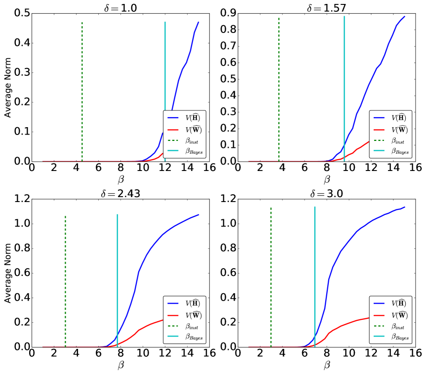
Figure 16: Normalized distances ${\sf V}({\widehat{\boldsymbol{H}}})$, ${\sf V}(\widehat{\boldsymbol{W}})$ of the AMP estimates from the uninformative fixed point. Here $k=3$, $d=1000$ and $n=d\delta$: each data point corresponds to an average over $400$ random realizations.

A

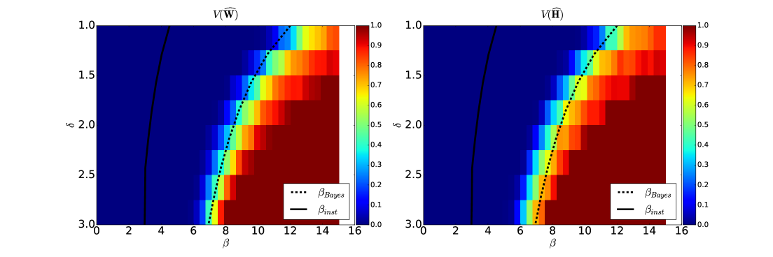
Figure 17: Empirical fraction of instances such that ${\sf V}(\widehat{\boldsymbol{W}})\geq{\varepsilon}_{0}=5\cdot 10^{-3}$ (left) or ${\sf V}({\widehat{\boldsymbol{H}}})\geq{\varepsilon}_{0}$ (right), where $\widehat{\boldsymbol{W}},{\widehat{\boldsymbol{H}}}$ are the AMP estimates. Here $k=3$, $d=1000$, and for each $(\delta,\beta)$ point on a grid we ran AMP on $400$ random realizations.

A

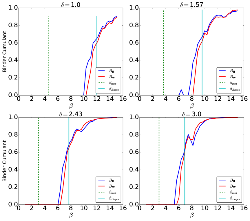
Figure 18: Binder cumulant for the correlation between AMP estimates $\widehat{\boldsymbol{W}},{\widehat{\boldsymbol{H}}}$ and the true weights and topics ${\boldsymbol{W}},{\boldsymbol{H}}$. Here $k=3$, $d=1000$, $n=d\delta$ and estimates are obtained by averaging over $400$ realizations.

A

Figure 19: Binder cumulant for the correlation between AMP estimates $\widehat{\boldsymbol{W}}$, ${\widehat{\boldsymbol{H}}}$ and the true weights and topics ${\boldsymbol{W}},{\boldsymbol{H}}$. Here $k=3$, $d=1000$ and estimates are obtained by averaging over $400$ realizations.

In Figures 16 to 19 we report our numerical results using damped AMP for the case of $k=3$ topics. These simulations are analogous to the one presented in the main text for $k=2$, cf. Section 4.5.

Figures 16 and 17 report results on the normalized distance from the uninformative subspace ${\sf V}({\widehat{\boldsymbol{H}}})$, ${\sf V}(\widehat{\boldsymbol{W}})$. These are consistent with the claim that AMP converges to a fixed point that is significantly distant from this subspace only if $\beta>\beta_{\mbox{\tiny\rm Bayes}}(k,\nu,\delta)=\beta_{\mbox{\tiny\rm spect}}(k,\nu,\delta)$. In Figures 18 and 19 we present our results on the correlation between the AMP estimates ${\widehat{\boldsymbol{H}}}$, $\widehat{\boldsymbol{W}}$ and the true factors ${\boldsymbol{H}}$, ${\boldsymbol{W}}$. We measure this correlation through the same Binder parameter introduced in Section E.2.

Appendix J Uniqueness of the solution to (3.13)

In this appendix, we prove that the solution to (3.13) is unique under the following conjecture

Conjecture J.1.

Let $q>0$ and ${\boldsymbol{w}}\in\mathbb{R}^{k}$ be a random variable with density $p({\boldsymbol{w}})\propto\exp\left\{-q\left\|{\boldsymbol{w}}\right\|_{2}^{2}\right\}\tilde{q}_{0}({\boldsymbol{w}})$. Then

$$\sigma(q)\gamma(q)\leq\frac{2}{q}$$ (J.1)

where $\sigma(q)$ and $\gamma(q)$ are the standard deviation and skewness of $\left\|{\boldsymbol{w}}\right\|_{2}^{2}$.

Remark J.1.

For a Gaussian random vector ${\boldsymbol{z}}\sim\mathcal{N}(0,(2q)^{-1}{\boldsymbol{I}}_{k})$ so that $p({\boldsymbol{z}})\propto\exp\left\{-q\left\|{\boldsymbol{z}}\right\|_{2}^{2}\right\}$,

$$\tilde{\sigma}(q)\tilde{\gamma}(q)=\frac{2}{q}$$ (J.2)

where $\tilde{\sigma}(q),\tilde{\gamma}_{1}(q)$ are the standard deviation and the skewness of $\left\|{\boldsymbol{z}}\right\|_{2}^{2}$.

Using the above conjecture, it can be shown that the solution to (3.13) is unique.

Let $V(q)$ be the variance of $X=\|{\boldsymbol{w}}\|_{2}^{2}$, when ${\boldsymbol{w}}$ is distributed with density $p({\boldsymbol{w}})\propto\exp\left\{-q\left\|{\boldsymbol{w}}\right\|_{2}^{2}\right\}\tilde{q}_{0}({\boldsymbol{w}})$. Define

$$f(q)=\frac{k\beta\delta}{k-1}\,\left\{{\sf E}\left(\frac{\beta}{1+q};\nu\right)-\frac{1}{k^{2}}\right\}\,.$$ (J.3)

Note that using the proof of Lemma (3.2), $f(q)$ is non-negative, continuous and monotone increasing for $q>0$. Further,

$$f^{\prime}(q)=\frac{\beta^{2}\delta}{(k-1)(1+q)^{2}}V\left(\frac{\beta}{1+q}\right).$$ (J.4)

Since $f(0)>0$, if we show that $f^{\prime}(q)$ is decreasing, then for $q>q^{*}$ where $q^{*}$ is the smallest solution to $f(q)=q$, $f^{\prime}(q)<1$. This will imply that $f(q)<q$ for $q>q^{*}$ that proves the uniqueness. We have

$$f^{\prime\prime}(q)=\frac{\beta^{2}\delta}{(k-1)(1+q)^{4}}\left[-\frac{\beta}{(1+q)^{2}}V^{\prime}\left(\frac{\beta}{1+q}\right)(1+q)^{2}-2(1+q)V\left(\frac{\beta}{1+q}\right)\right]$$ (J.5)

Hence, $f^{\prime}(q)$ is decreasing if and only if

$$-V^{\prime}\left(\frac{\beta}{1+q}\right)\leq 2\left(\frac{1+q}{\beta}\right)V\left(\frac{\beta}{1+q}\right).$$ (J.6)

Therefore, it is sufficient to show that for $q>0$,

$$\frac{-V^{\prime}(q)}{V(q)}\leq\frac{2}{q}.$$ (J.7)

Note that if we let $X=\|{\boldsymbol{w}}\|_{2}^{2}$ where ${\boldsymbol{w}}$ is as in Conjecture J.1, we have

$$V(q)={\mathbb{E}}(X^{2})-({\mathbb{E}}X)^{2}.$$ (J.8)

Further,

$$V^{\prime}(q) =-{\mathbb{E}}X^{3}+({\mathbb{E}}X)({\mathbb{E}}X^{2})-2({\mathbb{E}}X)\left[-{\mathbb{E}}X^{2}+({\mathbb{E}}X)^{2}\right]$$ (J.9)

$$=-{\mathbb{E}}X^{3}+3({\mathbb{E}}X^{2})({\mathbb{E}}X)-2({\mathbb{E}}X)^{3}.$$ (J.10)

Hence,

$$\frac{-V^{\prime}(q)}{V(q)}=\frac{{\mathbb{E}}(X^{3})-3({\mathbb{E}}X^{2})({\mathbb{E}}X)+2({\mathbb{E}}X)^{3}}{-{\mathbb{E}}X^{2}+({\mathbb{E}}X)^{2}}=\sigma(q)\gamma(q)\leq\frac{2}{q}$$ (J.11)

using Conjecture J.1. Therefore, $f(q)$ is concave and (3.13) has a unique solution in $q\in(0,\infty)$.

References

- [ABFX08] Edoardo M Airoldi, David M Blei, Stephen E Fienberg, and Eric P Xing, Mixed membership stochastic blockmodels, Journal of Machine Learning Research 9 (2008), no. Sep, 1981–2014.
- [AGKM12] Sanjeev Arora, Rong Ge, Ravindran Kannan, and Ankur Moitra, Computing a nonnegative matrix factorization–provably, Proceedings of the forty-fourth annual ACM symposium on Theory of computing, ACM, 2012, pp. 145–162.
- [AGM12] Sanjeev Arora, Rong Ge, and Ankur Moitra, Learning topic models–going beyond svd, Foundations of Computer Science (FOCS), 2012 IEEE 53rd Annual Symposium on, IEEE, 2012, pp. 1–10.
- [AGZ09] Greg W. Anderson, Alice Guionnet, and Ofer Zeitouni, An introduction to random matrices, Cambridge University Press, 2009.
- [AK18] Ahmed El Alaoui and Florent Krzakala, Estimation in the spiked wigner model: A short proof of the replica formula, arXiv preprint arXiv:1801.01593 (2018).
- [BBAP05] Jinho Baik, Gérard Ben Arous, and Sandrine Péché, Phase transition of the largest eigenvalue for nonnull complex sample covariance matrices, Annals of Probability (2005), 1643–1697.
- [BBW+13] Tamara Broderick, Nicholas Boyd, Andre Wibisono, Ashia C Wilson, and Michael I Jordan, Streaming variational bayes, Advances in Neural Information Processing Systems, 2013, pp. 1727–1735.
- [BCCZ13] Peter Bickel, David Choi, Xiangyu Chang, and Hai Zhang, Asymptotic normality of maximum likelihood and its variational approximation for stochastic blockmodels, The Annals of Statistics (2013), 1922–1943.
- [BDM+16] Jean Barbier, Mohamad Dia, Nicolas Macris, Florent Krzakala, Thibault Lesieur, and Lenka Zdeborová, Mutual information for symmetric rank-one matrix estimation: A proof of the replica formula, Advances in Neural Information Processing Systems, 2016, pp. 424–432.
- [BGN11] Florent Benaych-Georges and Raj Rao Nadakuditi, The eigenvalues and eigenvectors of finite, low rank perturbations of large random matrices, Advances in Mathematics 227 (2011), no. 1, 494–521.
- [BGN12] , The singular values and vectors of low rank perturbations of large rectangular random matrices, Journal of Multivariate Analysis 111 (2012), 120–135.
- [Bin81] Kurt Binder, Finite size scaling analysis of ising model block distribution functions, Zeitschrift für Physik B Condensed Matter 43 (1981), no. 2, 119–140.
- [BKM17] David M Blei, Alp Kucukelbir, and Jon D McAuliffe, Variational inference: A review for statisticians, Journal of the American Statistical Association (2017), no. just-accepted.
- [BL06] David M Blei and John D Lafferty, Dynamic topic models, Proceedings of the 23rd international conference on Machine learning, ACM, 2006, pp. 113–120.
- [BL07] , A correlated topic model of science, The Annals of Applied Statistics (2007), 17–35.
- [Ble12] David M Blei, Probabilistic topic models, Communications of the ACM 55 (2012), no. 4, 77–84.
- [BM11] Mohsen Bayati and Andrea Montanari, The dynamics of message passing on dense graphs, with applications to compressed sensing, IEEE Trans. on Inform. Theory 57 (2011), 764–785.
- [BMN17] Raphael Berthier, Andrea Montanari, and Phan-Minh Nguyen, State evolution for approximate message passing with non-separable functions, arXiv:1708.03950 (2017).
- [BNJ03] David M Blei, Andrew Y Ng, and Michael I Jordan, Latent dirichlet allocation, Journal of machine Learning research 3 (2003), no. Jan, 993–1022.
- [BS10] Z. Bai and J. Silverstein, Spectral Analysis of Large Dimensional Random Matrices, Springer, 2010.
- [CB09] Jonathan Chang and David Blei, Relational topic models for document networks, Artificial Intelligence and Statistics, 2009, pp. 81–88.
- [CDP+12] Alain Celisse, Jean-Jacques Daudin, Laurent Pierre, et al., Consistency of maximum-likelihood and variational estimators in the stochastic block model, Electronic Journal of Statistics 6 (2012), 1847–1899.
- [DAM17] Yash Deshpande, Emmanuel Abbe, and Andrea Montanari, Asymptotic mutual information for the balanced binary stochastic block model, Information and Inference: A Journal of the IMA 6 (2017), no. 2, 125–170.
- [DM14] Yash Deshpande and Andrea Montanari, Information-theoretically optimal sparse pca, Information Theory (ISIT), 2014 IEEE International Symposium on, IEEE, 2014, pp. 2197–2201.
- [DMM09] David L. Donoho, Arian Maleki, and Andrea Montanari, Message Passing Algorithms for Compressed Sensing, Proceedings of the National Academy of Sciences 106 (2009), 18914–18919.
- [DMM10] , Message Passing Algorithms for Compressed Sensing: I. Motivation and Construction, Proceedings of IEEE Inform. Theory Workshop (Cairo), 2010.
- [EFL04] Elena Erosheva, Stephen Fienberg, and John Lafferty, Mixed-membership models of scientific publications, Proceedings of the National Academy of Sciences 101 (2004), no. suppl 1, 5220–5227.
- [FFP05] Li Fei-Fei and Pietro Perona, A bayesian hierarchical model for learning natural scene categories, Computer Vision and Pattern Recognition, 2005. CVPR 2005. IEEE Computer Society Conference on, vol. 2, IEEE, 2005, pp. 524–531.
- [FP07] Delphine Féral and Sandrine Péché, The largest eigenvalue of rank one deformation of large wigner matrices, Communications in mathematical physics 272 (2007), no. 1, 185–228.
- [GBJ15] Ryan J Giordano, Tamara Broderick, and Michael I Jordan, Linear response methods for accurate covariance estimates from mean field variational bayes, Advances in Neural Information Processing Systems, 2015, pp. 1441–1449.
- [HBB10] Matthew Hoffman, Francis R Bach, and David M Blei, Online learning for Latent Dirichlet Allocation, Advances in neural information processing systems, 2010, pp. 856–864.
- [JGJS99] Michael I Jordan, Zoubin Ghahramani, Tommi S Jaakkola, and Lawrence K Saul, An introduction to variational methods for graphical models, Machine learning 37 (1999), no. 2, 183–233.
- [JM13] Adel Javanmard and Andrea Montanari, State evolution for general approximate message passing algorithms, with applications to spatial coupling, Information and Inference: A Journal of the IMA 2 (2013), no. 2, 115–144.
- [KF09] Daphne Koller and Nir Friedman, Probabilistic graphical models: principles and techniques, MIT press, 2009.
- [KM09] Satish Babu Korada and Nicolas Macris, Exact solution of the gauge symmetric p-spin glass model on a complete graph, Journal of Statistical Physics 136 (2009), no. 2, 205–230.
- [KXZ16] Florent Krzakala, Jiaming Xu, and Lenka Zdeborová, Mutual information in rank-one matrix estimation, IEEE Information Theory Workshop (ITW), 2016, pp. 71–75.
- [LB06] John D Lafferty and David M Blei, Correlated topic models, Advances in neural information processing systems, 2006, pp. 147–154.
- [LKZ17] Thibault Lesieur, Florent Krzakala, and Lenka Zdeborová, Constrained low-rank matrix estimation: Phase transitions, approximate message passing and applications, arXiv:1701.00858 (2017).
- [LM16] Marc Lelarge and Léo Miolane, Fundamental limits of symmetric low-rank matrix estimation, arXiv:1611.03888 (2016).
- [Mio17] Léo Miolane, Fundamental limits of low-rank matrix estimation, arXiv:1702.00473 (2017).
- [MM09] Marc Mézard and Andrea Montanari, Information, Physics and Computation, Oxford, 2009.
- [MPV87] Marc Mézard, Giorgio Parisi, and Miguel A. Virasoro, Spin glass theory and beyond, World Scientific, 1987.
- [MRZ17] Andrea Montanari, Daniel Reichman, and Ofer Zeitouni, On the limitation of spectral methods: From the gaussian hidden clique problem to rank one perturbations of gaussian tensors, IEEE Transactions on Information Theory 63 (2017), no. 3, 1572–1579.
- [MV17] Andrea Montanari and Ramji Venkataramanan, Estimation of low-rank matrices via approximate message passing, arXiv:1711.01682 (2017).
- [OW01] Manfred Opper and Ole Winther, Adaptive and self-averaging thouless-anderson-palmer mean-field theory for probabilistic modeling, Physical Review E 64 (2001), no. 5, 056131.
- [PBY17] Debdeep Pati, Anirban Bhattacharya, and Yun Yang, On statistical optimality of variational bayes, arXiv:1712.08983 (2017).
- [Per13] Lawrence Perko, Differential equations and dynamical systems, vol. 7, Springer Science & Business Media, 2013.
- [RRTB12] Ben Recht, Christopher Re, Joel Tropp, and Victor Bittorf, Factoring nonnegative matrices with linear programs, Advances in Neural Information Processing Systems, 2012, pp. 1214–1222.
- [RSP14] Anil Raj, Matthew Stephens, and Jonathan K Pritchard, faststructure: variational inference of population structure in large snp data sets, Genetics 197 (2014), no. 2, 573–589.
- [TAP77] David J. Thouless, Philip W. Anderson, and Richard G. Palmer, Solution of’solvable model of a spin glass’, Philosophical Magazine 35 (1977), no. 3, 593–601.
- [WB11] Chong Wang and David M Blei, Collaborative topic modeling for recommending scientific articles, Proceedings of the 17th ACM SIGKDD international conference on Knowledge discovery and data mining, ACM, 2011, pp. 448–456.
- [WG08] Xiaogang Wang and Eric Grimson, Spatial latent dirichlet allocation, Advances in neural information processing systems, 2008, pp. 1577–1584.
- [WJ08] Martin J Wainwright and Michael I Jordan, Graphical models, exponential families, and variational inference, Foundations and Trends in Machine Learning 1 (2008), no. 1-2, 1–305.
- [WT04] Bo Wang and D. Michael Titterington, Convergence and asymptotic normality of variational Bayesian approximations for exponential family models with missing values, Proceedings of the 20th conference on Uncertainty in artificial intelligence, AUAI Press, 2004, pp. 577–584.
- [WT05] , Inadequacy of interval estimates corresponding to variational Bayesian approximations, AISTATS, 2005.
- [WT06] , Convergence properties of a general algorithm for calculating variational Bayesian estimates for a normal mixture model, Bayesian Analysis 1 (2006), no. 3, 625–650.
- [ZBHD15] Jing Zhou, Anirban Bhattacharya, Amy H Herring, and David B Dunson, Bayesian factorizations of big sparse tensors, Journal of the American Statistical Association 110 (2015), no. 512, 1562–1576.
- [ZZ17] Anderson Y Zhang and Harrison H Zhou, Theoretical and computational guarantees of mean field variational inference for community detection, arXiv:1710.11268 (2017).