Trimaximal mixing with a texture zero

Abstract

We analyze neutrino mass matrices having one texture zero, assuming that the neutrino mixing matrix has either its first (TM₁) or second (TM₂) column identical to that of the tribimaximal mixing matrix. We found that all the six possible one texture zero neutrino mass matrices are compatible with the present neutrino oscillation data when combined with TM₁ or TM₂ mixing. These textures have interesting predictions for the presently unknown parameters such as the effective Majorana neutrino mass, the Dirac CP violating phase and the neutrino mass scale. We also present a way to theoretically realize some of these textures using $A_{4}$ symmetry within the framework of type-I+II seesaw mechanism.

I Introduction

Various neutrino oscillation experiments in the last decade or so have measured the three lepton mixing angles and it is now clear that the flavor mixing in the lepton sector is quite large as compared to the quark sector. Non-Abelian discrete flavor symmetries have been extensively utilized to explain the large mixing in the lepton sector discrete . Among the most widely studied lepton mixing patterns obtained using discrete non-Abelian symmetries is the tribimaximal (TBM) mixing pattern tbm

$$U_{TBM}=\left(\begin{array}[]{ccc}-\frac{\sqrt{2}}{\sqrt{3}}&\frac{1}{\sqrt{3}}&0\\ \frac{1}{\sqrt{6}}&\frac{1}{\sqrt{3}}&-\frac{1}{\sqrt{2}}\\ \frac{1}{\sqrt{6}}&\frac{1}{\sqrt{3}}&\frac{1}{\sqrt{2}}\end{array}\right)$$ (1)

which predicts the reactor mixing angle $\theta_{13}$ to be zero, a maximal atmospheric mixing angle, i.e., $\theta_{23}=\frac{\pi}{4}$, and the solar mixing angle $\theta_{12}=\sin^{-1}(1/\sqrt{3})$. However, recent neutrino oscillation experiments have found $\theta_{13}$ to be non-zero th13 , necessitating some modifications to the TBM mixing scheme to make it compatible with the present experimental data. In this context it has been observed that the first or the second column of TBM mixing matrix can still accommodate the recent neutrino oscillation data He . When the second column of TBM mixing matrix remains intact while the other columns deviate from TBM values we denote that mixing matrix as TM₂ WR . Similarly, if the first column of TBM remains intact and other columns deviate from TBM we denote it by TM₁ WR . When either of these columns of TBM remain intact in the lepton mixing matrix we can parametrize the mixing matrix in terms of one mixing angle and one CP violating Dirac phase along with two Majorana phases He ; WR .
There are many other approaches which have been used to explain neutrino mixing, some of these are: texture zeros tz , vanishing cofactors cofactor , hybrid textures hybrid etc. Out of these, texture zeros have been quite successful in explaining mixing in both the quark and the lepton sectors. In the basis where the charged lepton mass matrix is diagonal there are seven patterns of two texture zeros which are compatible with the current neutrino oscillation data tz . There are six possible patterns of one texture zero in the neutrino mass matrix which are shown in Table 1. All of these are compatible with the present experimental data onezero .
Neutrino mass matrices with two texture zeros in combination with TM₂ mixing have been studied in Ref. ourtm2 where it has been found that only two patterns namely $A_{1}$ and $A_{2}$ (with texture zeros at (1,1), (1,2) and (1,1), (1,3) entries, respectively) can satisfy the present experimental data when we combine two texture zeros with TM₂ mixing. The combination of TM₁ mixing with two texture zeros has been studied in Ref. ourtm1 and similar to the TM₂ case it has been found that only patterns $A_{1}$ and $A_{2}$ of two texture zeros are compatible with the present neutrino oscillation data when combined with TM₁ mixing. This approach of combining texture zeros with TM₁/TM₂ mixing turns out to be very fruitful as it leads to very predictive texture structures of neutrino mass matrix. In the present work we study neutrino mass matrices having one texture zero in combination with TM₂/TM₁ mixing.

Pattern	Constraining Equation
I	$M_{ee}=0$
II	$M_{e\mu}=0$
III	$M_{e\tau}=0$
IV	$M_{\mu\mu}=0$
V	$M_{\mu\tau}=0$
VI	$M_{\tau\tau}=0$

Table 1: Six allowed patterns of one texture zero in the neutrino mass matrix.

II TM₂ Mixing and one texture zero

II.1 TM₂ Mixing

A neutrino mass matrix with TBM mixing can be diagonalized as

$$M_{\text{diag}}=U_{TBM}^{T}M_{TBM}U_{TBM}$$ (2)

where $U_{TBM}$ contains the eigenvectors $t=(-\frac{\sqrt{2}}{\sqrt{3}}~{}\frac{1}{\sqrt{6}}~{}\frac{1}{\sqrt{6}})^{T}$, $u=(\frac{1}{\sqrt{3}}~{}\frac{1}{\sqrt{3}}~{}\frac{1}{\sqrt{3}})^{T}$ and $v=(0~{}\frac{-1}{\sqrt{2}}~{}\frac{1}{\sqrt{2}})^{T}$. The diagonal matrix $M_{\text{diag}}$ is given as

$$M_{\text{diag}}=\left(\begin{array}[]{ccc}m_{1}&0&0\\ 0&e^{2i\alpha}m_{2}&0\\ 0&0&e^{2i\beta}m_{3}\end{array}\right),$$ (3)

where $m_{1}$, $m_{2}$, and $m_{3}$ are the three neutrino masses and $\alpha$ and $\beta$ are the two Majorana phases. The mass matrix $M_{TBM}$ is invariant under the transformations $G_{t}$, $G_{u}$ and $G_{v}$; i.e. $G_{t}^{T}M_{TBM}G_{t}=M_{TBM}$, $G_{u}^{T}M_{TBM}G_{u}=M_{TBM}$ and $G_{v}^{T}M_{TBM}G_{v}=M_{TBM}$ with $G_{t}=1-2tt^{T}$, $G_{u}=1-2uu^{T}$ and $G_{v}=1-2vv^{T}$. The transformation matrices $G_{u}$ and $G_{v}$ correspond to the magic symmetry Lam and the $\mu-\tau$ symmetry Lam , respectively. $G_{i}~{}(i=t,u,v)$ are generators of $Z_{2}$ group. A $3\times 3$ neutrino mass matrix with TBM symmetry is invariant under the $Z^{t}_{2}\times Z^{u}_{2}\times Z^{v}_{2}$ group. Recently, neutrino oscillation experiments have confirmed a non-zero $\theta_{13}$, thus, the neutrino mass matrix $M_{\nu}$ cannot remain invariant under the $\mu-\tau$ symmetry transformation $G_{v}$. However, the neutrino mass matrix can still be invariant under the magic symmetry transformation $G_{u}$ as the experimental data are still compatible with the magic symmetry. The mixing matrix which corresponds to the magic symmetry is known as the trimaximal mixing (TM₂) matrix and can be parametrized as He ; WR ; Bjorken ; Lam ; SK

$$U_{\textrm{TM}_{2}}=\left(\begin{array}[]{ccc}\sqrt{\frac{2}{3}}\cos\theta&\frac{1}{\sqrt{3}}&\sqrt{\frac{2}{3}}\sin\theta\\ -\frac{\cos\theta}{\sqrt{6}}+\frac{e^{-i\phi}\sin\theta}{\sqrt{2}}&\frac{1}{\sqrt{3}}&-\frac{\sin\theta}{\sqrt{6}}-\frac{e^{-i\phi}\cos\theta}{\sqrt{2}}\\ -\frac{\cos\theta}{\sqrt{6}}-\frac{e^{-i\phi}\sin\theta}{\sqrt{2}}&\frac{1}{\sqrt{3}}&-\frac{\sin\theta}{\sqrt{6}}+\frac{e^{-i\phi}\cos\theta}{\sqrt{2}}\end{array}\right).$$ (4)

The TM₂ mixing matrix has its middle column fixed to the TBM value ($u$), which leaves only two free parameters ($\theta$ and $\phi$) in $U_{\text{TM}_{2}}$ after we take into account the unitarity constraints. The neutrino mass matrix corresponding to TM₂ mixing is given as

$$M_{\textrm{TM}_{2}}=U_{\text{TM}_{2}}^{*}M_{\text{diag}}U_{\text{TM}_{2}}^{\dagger}.$$ (5)

II.2 One zero in $M_{\text{TM}_{2}}$

A neutrino mass matrix with TM₂ mixing can be parameterized as magic

$$M_{\textrm{TM}_{2}}=\left(\begin{array}[]{ccc}a&b&c\\ b&d&a+c-d\\ c&a+c-d&b-c+d\end{array}\right).$$ (6)

The constraint equations for all the patterns with one texture zero and TM₂ mixing can be obtained by substituting the respective texture zero constraints from Table 1 into Eq. (6). In the diagonal charged lepton mass matrix basis, all the six patterns of one texture zero in the neutrino mass matrix are compatible with the present experimental data. The combination of these one texture zero patterns with TM₂ mixing is bound to produce very predictive forms of neutrino mass matrices.
The neutrino mass matrices with one texture zero and TM₂ mixing are given below:

$$M^{\textrm{I}}_{\textrm{TM}_{2}}=\left(\begin{array}[]{ccc}0&b&c\\ b&d&c-d\\ c&c-d&b-c+d\end{array}\right)$$ (7)

$$M^{\textrm{II}}_{\textrm{TM}_{2}}=\left(\begin{array}[]{ccc}a&0&c\\ 0&d&a+c-d\\ c&a+c-d&-c+d\end{array}\right)$$ (8)

$$M^{\textrm{III}}_{\textrm{TM}_{2}}=\left(\begin{array}[]{ccc}a&b&0\\ b&d&a-d\\ 0&a-d&b+d\end{array}\right)$$ (9)

$$M^{\textrm{IV}}_{\textrm{TM}_{2}}=\left(\begin{array}[]{ccc}a&b&c\\ b&0&a+c\\ c&a+c&b-c\end{array}\right)$$ (10)

$$M^{\textrm{V}}_{\textrm{TM}_{2}}=\left(\begin{array}[]{ccc}a&b&c\\ b&a+c&0\\ c&0&a+b\end{array}\right)$$ (11)

$$M^{\textrm{VI}}_{\textrm{TM}_{2}}=\left(\begin{array}[]{ccc}a&b&c\\ b&c-b&a+b\\ c&a+b&0\end{array}\right)$$ (12)

The above mass matrices [Eq. (7) to Eq. (12)] can be rewritten as:

$$M^{\textrm{I}}_{\textrm{TM}_{2}}=\left(\begin{array}[]{ccc}0&b&c\\ b&c-\Delta&\Delta\\ c&\Delta&b-\Delta\end{array}\right)\ \ \ \textrm{where}\ \ \ \Delta=c-d$$ (13)

$$M^{\textrm{II}}_{\textrm{TM}_{2}}=\left(\begin{array}[]{ccc}a&0&c\\ 0&c-\Delta&a+\Delta\\ c&a+\Delta&-\Delta\end{array}\right)\ \ \ \textrm{where}\ \ \ \Delta=c-d$$ (14)

$$M^{\textrm{III}}_{\textrm{TM}_{2}}=\left(\begin{array}[]{ccc}a&b&0\\ b&d&a-d\\ 0&a-d&b+d\end{array}\right)$$ (15)

$$M^{\textrm{IV}}_{\textrm{TM}_{2}}=\left(\begin{array}[]{ccc}\Lambda-c&b&c\\ b&0&\Lambda\\ c&\Lambda&b-c\end{array}\right)\ \ \ \textrm{where}\ \ \ \Lambda=a+c$$ (16)

$$M^{\textrm{V}}_{\textrm{TM}_{2}}=\left(\begin{array}[]{ccc}a&\Omega-a&c\\ \Omega-a&a+c&0\\ c&0&\Omega\end{array}\right)\ \ \ \textrm{where}\ \ \ \Omega=a+b$$ (17)

$$M^{\textrm{VI}}_{\textrm{TM}_{2}}=\left(\begin{array}[]{ccc}\Omega-b&b&c\\ b&c-b&\Omega\\ c&\Omega&0\end{array}\right)\ \ \ \textrm{where}\ \ \ \Omega=a+b$$ (18)

All the six patterns from Eq. (13) to Eq. (18) can be written as a linear combination of following matrices

$$p_{12}=\left(\begin{array}[]{ccc}0&1&0\\ 1&0&0\\ 0&0&1\end{array}\right),\ \ \ p_{13}=\left(\begin{array}[]{ccc}0&0&1\\ 0&1&0\\ 1&0&0\end{array}\right),$$ (25)

$$p_{23}=\left(\begin{array}[]{ccc}1&0&0\\ 0&0&1\\ 0&1&0\end{array}\right),\ \ \ b_{12}=\left(\begin{array}[]{ccc}-1&1&0\\ 1&-1&0\\ 0&0&0\end{array}\right),$$ (32)

$$b_{13}=\left(\begin{array}[]{ccc}-1&0&1\\ 0&0&0\\ 1&0&-1\end{array}\right),\ \ \ b_{23}=\left(\begin{array}[]{ccc}0&0&0\\ 0&-1&1\\ 0&1&-1\end{array}\right),$$ (39)

where the first three are the symmetric permutation matrices and the last three are in block diagonal form, e.g. $M^{\textrm{I}}_{\textrm{TM}_{2}}$ is obtained as a linear combination of $p_{12}$, $p_{13}$ and $b_{23}$:

$$M^{\textrm{I}}_{\textrm{TM}_{2}}=\Delta\ b_{23}+b\ p_{12}+c\ p_{13}.$$ (40)

Similarly, we can construct other patterns. This representation brings all the patterns on equal footing; i.e., all the one texture zero patterns with TM₂ mixing are made up of simple combinations of two symmetric permutation matrices and a block diagonal matrix. The above decomposition into permutation and block diagonal matrices also helps in the symmetry realization of these patterns.
A neutrino mass matrix with TM₂ mixing is diagonalized by the mixing matrix $U=U_{\textrm{TM}_{2}}$ given in Eq. (4).

$$U_{\textrm{TM}_{2}}^{T}M_{\textrm{TM}_{2}}U_{\textrm{TM}_{2}}=M_{\textrm{diag.}}.$$ (41)

We can calculate the neutrino mixing angles from a given mixing matrix $U$ by using the following relations:

$$s_{12}^{2}=\frac{|U_{12}|^{2}}{1-|U_{13}|^{2}},s_{23}^{2}=\frac{|U_{23}|^{2}}{1-|U_{13}|^{2}},\textrm{ and }s_{13}^{2}=|U_{13}|^{2}.$$ (42)

The mixing angles for TM₂ mixing in terms of parameters $\theta$ and $\phi$ are

$$s_{12}^{2}= \frac{1}{3-2\sin^{2}\theta},\ \ \ s_{13}^{2}=\frac{2}{3}\sin^{2}\theta.$$

$$s_{23}^{2}= \frac{1}{2}\left(1+\frac{\sqrt{3}\sin 2\theta\cos\phi}{3-2\sin^{2}\theta}\right).$$ (43)

The Dirac CP violating phase $\delta$ can be obtained from the Jarlskog rephasing invariant ($J_{CP}$) jcp

$$J_{CP}=\textrm{Im}(U_{11}U_{12}^{*}U_{21}^{*}U_{22}).$$ (44)

In the standard parametrization

$$J_{CP}=s_{12}s_{23}s_{13}c_{12}c_{23}c_{13}^{2}\sin\delta.$$ (45)

For the TM₂ mixing matrix

$$J_{CP}=\frac{1}{6\sqrt{3}}\sin 2\theta\sin\phi.$$ (46)

From Eqs. (45) and (46), we obtain

$$\tan\delta=\frac{\cos 2\theta+2}{2\cos 2\theta+1}\tan\phi.$$ (47)

The effective Majorana mass term relevant for neutrinoless double beta decay is given by

$$|M_{ee}|=|m_{1}U^{2}_{e1}+m_{2}e^{2i\alpha}U^{2}_{e2}+m_{3}e^{2i\beta}U^{2}_{e3}|.$$ (48)

For TM₂ mixing, the above expression takes the following form

$$|M_{ee}|=\frac{1}{3}|2m_{1}\cos^{2}\theta+m_{2}e^{2i\alpha}+2m_{3}e^{2i\beta}\sin^{2}\theta|.$$ (49)

There are many ongoing and forthcoming experiments such as GERDA gerda , CUORE coure , EXO exo , NEXT next , MAJORANA majorana , SuperNEMO supernemo which aim to achieve a sensitivity up to 0.01 eV for $|M_{ee}|$. Cosmological observations put an upper bound on the sum of neutrino masses

$$\Sigma=\sum_{i=1,2,3}^{3}m_{i}.$$ (50)

Planck satellite data planck combined with WMAP, CMB and BAO experiments limit the sum of neutrino masses $\sum m_{i}\leq 0.23$ eV at 95$\%$ confidence level (CL). In the present work, we assume a more conservative limit of $\sum m_{i}\leq 1$ eV. The existence of one texture zero in the neutrino mass matrix with TM₂ mixing implies

$$(M_{\textrm{TM}_{2}})_{ij}=0.$$ (51)

This condition yields a complex equation viz.

$$m_{1}A+m_{2}B+m_{3}C=0$$ (52)

where, $A=U_{a1}U_{b1}$, $B=U_{a2}U_{b2}e^{2i\alpha}$, $C=U_{a3}U_{b3}e^{2i\beta}$ and $a$, $b$ can take values $e$, $\mu$ and $\tau$. The above complex equation yields two mass ratios:

$$\frac{m_{1}}{m_{2}}=\frac{\textrm{Re}(C)\textrm{Im}(B)-\textrm{Re}(B)\textrm{Im}(C)}{\textrm{Re}(A)\textrm{Im}(C)-\textrm{Re}(C)\textrm{Im}(A)}$$ (53)

and

$$\frac{m_{1}}{m_{3}}=\frac{\textrm{Re}(C)\textrm{Im}(B)-\textrm{Re}(B)\textrm{Im}(C)}{\textrm{Re}(B)\textrm{Im}(A)-\textrm{Re}(A)\textrm{Im}(B)}$$ (54)

where Re (Im) denotes the real (imaginary) part. These mass ratios can be used to obtain the expression for the parameter $R_{\nu}$, which is the ratio of mass squared differences ($\Delta m_{ij}^{2}=m_{i}^{2}-m_{j}^{2}$):

$$R_{\nu}\equiv\frac{\Delta m_{21}^{2}}{|\Delta m_{31}^{2}|}=\frac{(\frac{m_{2}}{m_{1}})^{2}-1}{|(\frac{m_{3}}{m_{1}})^{2}-1|}$$ (55)

where $m_{1}>m_{3}$ for an inverted mass ordering (IO) and $m_{1}<m_{3}$ for the normal mass ordering (NO). For a texture zero to be compatible with the present neutrino oscillation data, the parameter $R_{\nu}$ should lie within its experimentally allowed range. The phenomenological predictions of patterns $M^{\textrm{II}}_{\textrm{TM}_{2}}$ and $M^{\textrm{III}}_{\textrm{TM}_{2}}$ are related and one can obtain the predictions for pattern $M^{\textrm{III}}_{\textrm{TM}_{2}}$ by making the following transformations:

$$\theta_{23}\rightarrow\frac{\pi}{2}-\theta_{23},\ \ \ \delta=\pi-\delta$$ (56)

on the predictions of pattern $M^{\textrm{II}}_{\textrm{TM}_{2}}$ and vice-versa. This is because patterns $M^{\textrm{III}}_{\textrm{TM}_{2}}$ and $M^{\textrm{II}}_{\textrm{TM}_{2}}$ are related via 2-3 symmetry: $M^{\textrm{III}}_{\textrm{TM}_{2}}=p_{23}^{T}M^{\textrm{II}}_{\textrm{TM}_{2}}p_{23}$ where $p_{23}$ is the 2-3 permutation matrix given in Eq. (25). Similarly, patterns $M^{\textrm{IV}}_{\textrm{TM}_{2}}$ and $M^{\textrm{VI}}_{\textrm{TM}_{2}}$ are related to each other by above transformations. Thus, we need to study in detail only one of the 2-3 symmetry related patterns.
In the numerical analysis, the neutrino mass matrix is reconstructed using Eq. (5), which takes into account the constraint of TM₂ mixing. For the numerical analysis we generate $10^{8}$ points ($10^{10}$ for pattern $M^{\textrm{V}}_{\textrm{TM}_{2}}$ with NO). The mass squared differences $\Delta m_{21}^{2}$ and $|\Delta m_{31}^{2}|$ are varied randomly within their 3$\sigma$ experimental ranges. Parameters $\theta$, $\phi$, $\alpha$ and $\beta$ are varied randomly within their full possible ranges. The texture zero constraint is imposed by requiring that the parameter $R_{\nu}$ in Eq. (55), written in terms of mass ratios $\frac{m_{1}}{m_{2}}$ and $\frac{m_{1}}{m_{3}}$ should lie within its 3$\sigma$ experimental range. In addition to above constraints, we require the allowed points to lie within the 3$\sigma$ experimental ranges of mixing angles $\theta_{12}$, $\theta_{13}$ and $\theta_{23}$ where the neutrino mixing angles are extracted by using the relations given in Eq. (42). The experimental ranges of various neutrino oscillation parameters with their 1, 2, 3$\sigma$ ranges are given in Table 2.

Parameter	Normal Ordering	Inverted Ordering
	best fit $\pm 1\sigma,\pm 2\sigma$    $3\sigma$ range	best fit $\pm 1\sigma,\pm 2\sigma$       $3\sigma$ range
$\theta_{12}^{\circ}$	$34.5^{+1.1,+2.3}_{-1.0,-2.0}$    $31.5$ - $38.0$	$34.5^{+1.1,+2.3}_{-1.0,-2.0}$        $31.5$ - $38.0$
$\theta_{23}^{\circ}$	$41.0^{+1.1,+2.7}_{-1.1,-1.9}$   $38.3$ - $52.8$	$50.5^{+1.0,+1.7}_{-1.0,-2.3}$        $38.5$ - $53.0$
$\theta_{13}^{\circ}$	$8.44^{+0.18,+0.26}_{-0.15,-0.34}$   $7.9$ - $8.9$	$8.41^{+0.16,+0.29}_{-0.17,-0.41}$        $7.9$ - $8.93$
$\delta_{CP}^{\circ}$	$252^{+56,+99}_{-36,-99}$    $0.0$ - $360$	$259^{+47,+88}_{-41,-77}$      $0$ - $31$ $\oplus$ $142$ - $360$
$\Delta m^{2}_{21}/10^{-5}eV^{2}$	$7.56^{+0.19,+0.39}_{-0.19,-0.36}$   $7.05$ - $8.14$	$7.56^{+0.19,+0.39}_{-0.19,-0.36}$        $7.05$ - $8.14$
$|\Delta m^{2}_{3l}|/10^{-3}eV^{2}$	$2.55^{+0.04,+0.08}_{-0.04,-0.08}$    $2.43$ - $2.67$	$2.49^{+0.04,+0.08}_{-0.04,-0.08}$        $2.37$ - $2.61$

Table 2: Current neutrino oscillation parameters from global fits data .

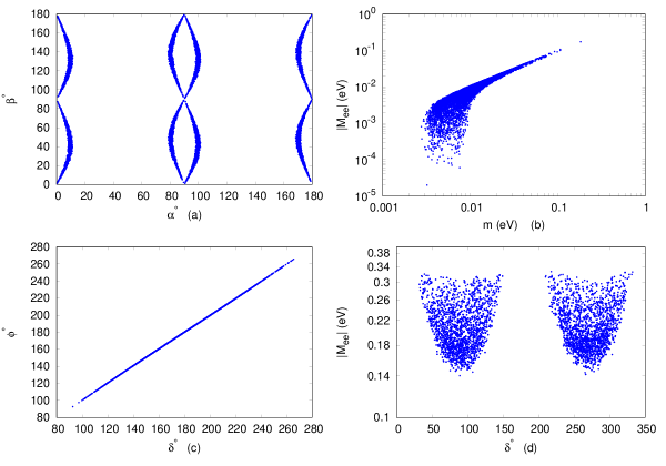
Figure 1: Correlation plots for patterns $M^{\textrm{I}}_{\text{TM}_{2}}$ (a), $M^{\textrm{II}}_{\text{TM}_{2}}$ (b), $M^{\textrm{IV}}_{\text{TM}_{2}}$ (c) and $M^{\textrm{V}}_{\text{TM}_{2}}$ (d) with NO.

The numerical results for one texture zero in the neutrino mass matrix with TM₂ mixing are presented below. The main observations are:

1. All six patterns of one texture zero in the neutrino mass matrix with TM₂ mixing are consistent with the present neutrino oscillation data.

2. The pattern $M^{\textrm{I}}_{\textrm{TM}_{2}}$ is consistent with normal mass ordering only.

3. All the viable patterns except $M^{\textrm{I}}_{\textrm{TM}_{2}}$, allow a quasidegenerate mass spectrum.

4. In case of NO, the parameter $|M_{ee}|$ can vanish for patterns $M^{\textrm{I}}_{\textrm{TM}_{2}}$, $M^{\textrm{II}}_{\textrm{TM}_{2}}$ and $M^{\textrm{III}}_{\textrm{TM}_{2}}$. For the remaining patterns $|M_{ee}|$ is found to be bounded from below.

5. The smallest neutrino mass cannot vanish except for patterns $M^{\textrm{II}}_{\textrm{TM}_{2}}$ and $M^{\textrm{III}}_{\textrm{TM}_{2}}$ with IO.

6. The parameter $J_{CP}$ cannot vanish for patterns $M^{\textrm{II}}_{\text{TM}_{2}}$ with IO and $M^{\textrm{V}}_{\text{TM}_{2}}$ with NO, implying that these patterns are necessarily CP violating.

7. The atmospheric neutrino mixing angle $\theta_{23}$ remains below (above) 45^∘ for pattern $M^{\textrm{IV}}_{\textrm{TM}_{2}}$ ($M^{\textrm{VI}}_{\textrm{TM}_{2}}$) with NO.

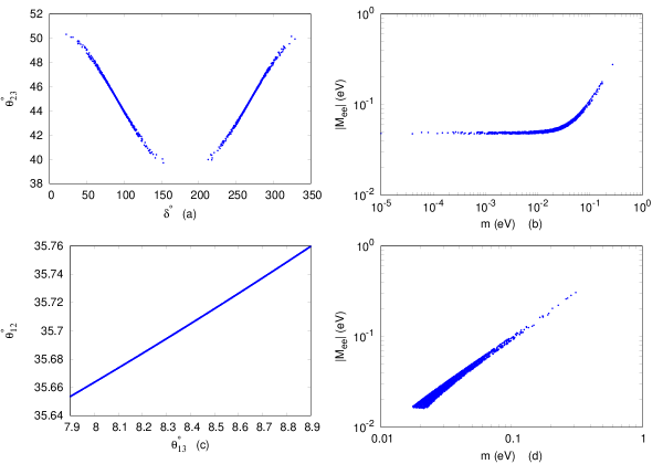
Figure 2: Correlation plots for patterns $M^{\textrm{II}}_{\text{TM}_{2}}$ (a,b), $M^{\textrm{IV}}_{\text{TM}_{2}}$ (c) and $M^{\textrm{V}}_{\text{TM}_{2}}$ (d) with IO.

Figure 3: Correlation plots for patterns $M^{\textrm{IV}}_{\text{TM}_{2}}$ (a) and $M^{\textrm{VI}}_{\text{TM}_{2}}$ (b) with NO.

The numerical predictions for the presently unknown neutrino parameters have been summarized in Table 3. The allowed ranges (at 3$\sigma$ CL) of parameters $\theta_{12}$, $\theta$ and $J_{CP}$ are ($35.65^{\circ}$ - $35.76^{\circ}$), ($9.68^{\circ}$ - $10.93^{\circ}$) and ($-0.0363$ - $0.0363$), respectively, for all the allowed patterns except for patterns $M^{\textrm{II,\ III}}_{\text{TM}_{2}}$ with IO and $M^{\textrm{V}}_{\text{TM}_{2}}$ with NO, for which $J_{CP}$ cannot vanish and has the allowed ranges $\pm$($0.006$ - $0.036$) and $\pm$($0.0165$ - $0.036$), respectively. Some of the interesting correlation plots are given in Figs. 1, 2 and 3. Fig. 1(a) shows that the Majorana phases $\alpha$ and $\beta$ are strongly correlated with each other for pattern $M^{\textrm{I}}_{\text{TM}_{2}}$ with NO. One can see from Fig. 1(c) that the Dirac phase $\delta$ and phase $\phi$ are linearly correlated and are almost identical to each other. From Eq. (47) we can see that the ratio $(\frac{\cos 2\theta+2}{2\cos 2\theta+1})$ multiplying with $\tan\phi$ remains $\approx 1$ for the allowed values of $\theta$. This leads to the feature $\delta\approx\phi$, for all the neutrino mass matrices with a texture zero and TM₂ mixing.
For pattern $M^{\textrm{II}}_{\text{TM}_{2}}$ the Dirac phase $\delta$ is restricted to two regions [Fig. 2(a)]. The correlation between mixing angles $\theta_{13}$ and $\theta_{12}$ is shown in Fig. 2(c). This is a generic feature of TM₂ mixing arising from Eq. (II.2). Since the TBM value of $\theta_{12}$ is already above its experimental best fit value, an increase in $\theta$ drives $\theta_{12}$ further away from the best fit experimental value. Thus, TM₂ mixing leads to some tension with mixing angle $\theta_{12}$. Fig. 3 shows the 2-3 symmetry between patterns $M^{\textrm{IV}}_{\text{TM}_{2}}$ and $M^{\textrm{VI}}_{\text{TM}_{2}}$.

Pattern	Mass Ordering	$|M_{ee}|$ (eV)	Lightest Neutrino Mass $m$ (eV)	$\sum m_{i}$ (eV)	$\delta^{\circ}$
I	NO	$0.0$	$0.0026$ - $0.0084$	$0.061$ - $0.073$	$0$ - $360$
II	NO	$0.0$ - $0.172$	$0.002$ - $0.183$	$0.056$ - $0.57$	$0$ - $360$
	IO	$0.047$ - $0.275$	$0.0$ - $0.272$	$0.097$ - $0.825$	$21$ - $154$ $\oplus$ $200$ - $345$
III	NO	$0.0$ - $0.172$	$0.002$ - $0.183$	$0.056$ - $0.57$	$0$ - $360$
	IO	$0.047$ - $0.275$	$0.0$ - $0.272$	$0.097$ - $0.825$	$29$ - $159$ $\oplus$ $200$ - $332$
IV	NO	$0.034$ - $0.237$	$0.035$ - $0.3$	$0.13$ - $0.9$	$90$ - $270$
	IO	$0.015$ - $0.126$	$0.007$ - $0.18$	$0.106$ - $0.553$	$0$ - $360$
V	NO	$0.14$ - $0.34$	$0.147$ - $0.332$	$0.45$ - $1$	$32$ - $150$ $\oplus$ $209$ - $333$
	IO	$0.015$ - $0.305$	$0.017$ - $0.31$	$0.127$ - $0.94$	$0$ - $360$
VI	NO	$0.034$ - $0.237$	$0.035$ - $0.3$	$0.13$ - $0.9$	$0$ - $90$ $\oplus$ $270$ - $360$
	IO	$0.015$ - $0.126$	$0.007$ - $0.18$	$0.106$ - $0.553$	$0$ - $360$

Table 3: Numerical predictions (at 3$\sigma$ CL) for patterns having one texture zero in $M_{\nu}$ with TM₂ mixing.

II.3 Symmetry realization

The neutrino mass matrices with one texture zero and TM₂ mixing can be realized in the framework of type-I+II seesaw mechanism seesaw1 ; seesaw2 using $A_{4}$ a4 symmetry. In addition to the three standard model lepton $SU(2)_{L}$ doublets $D_{l_{L}}$ (where $l=e,\mu~{}\text{and}~{}\tau$) and three right-handed charged lepton singlets $l_{R}$, we need a $SU(2)_{L}$ singlet right-handed neutrino $\nu_{R}$, six $SU(2)_{L}$ doublet Higgs fields $\psi_{i}$ and $\varphi_{i}$ ($i=1,2,3$), and two $SU(2)_{L}$ triplet Higgs fields $\Delta_{1}$, $\Delta_{2}$. We also impose an additional $Z_{2}$ symmetry, to prevent couplings between charged leptons (neutrinos) and scalars $\varphi_{i}$ ($\psi_{i}$). Below we discuss in detail the symmetry realization of pattern $M^{\textrm{I}}_{\text{TM}_{2}}$. The transformation properties of various fields under $A_{4}$ and $Z_{2}$ corresponding to pattern I are given in Table 4. These transformation properties lead to the following Yukawa Lagrangian which is invariant under $A_{4}$ and $Z_{2}$.

$$-\mathcal{L}_{\text{Yukawa}} = y_{1}(\overline{D}_{e_{L}}\psi_{1}+\overline{D}_{\mu_{L}}\psi_{2}+\overline{D}_{\tau_{L}}\psi_{3})_{\underline{1}}e_{R_{\underline{1}}}+y_{2}(\overline{D}_{e_{L}}\psi_{1}+\omega^{2}\overline{D}_{\mu_{L}}\psi_{2}+\omega\overline{D}_{\tau_{L}}\psi_{3})_{\underline{1}^{\prime}}\tau_{R_{\underline{1}^{\prime\prime}}}$$ (57)

$$+ y_{3}(\overline{D}_{e_{L}}\psi_{1}+\omega\overline{D}_{\mu_{L}}\psi_{2}+\omega^{2}\overline{D}_{\tau_{L}}\psi_{3})_{\underline{1}^{\prime\prime}}\mu_{R_{\underline{1}^{\prime}}}+y_{4}(\overline{D}_{e_{L}}\tilde{\varphi}_{1}+\overline{D}_{\mu_{L}}\tilde{\varphi}_{2}+\overline{D}_{\tau_{L}}\tilde{\varphi}_{3})_{\underline{1}}\nu_{R_{\underline{1}}}$$

$$- y_{\Delta_{1}}(D_{e_{L}}^{T}C^{-1}D_{e_{L}}+\omega D_{\mu_{L}}^{T}C^{-1}D_{\mu_{L}}+\omega^{2}D_{\tau_{L}}^{T}C^{-1}D_{\tau_{L}})_{\underline{1}^{\prime\prime}}i\tau_{2}\Delta_{1_{\underline{1}^{\prime}}}$$

$$- y_{\Delta_{2}}(D_{e_{L}}^{T}C^{-1}D_{e_{L}}+\omega^{2}D_{\mu_{L}}^{T}C^{-1}D_{\mu_{L}}+\omega D_{\tau_{L}}^{T}C^{-1}D_{\tau_{L}})_{\underline{1}^{\prime}}i\tau_{2}\Delta_{2_{\underline{1}^{\prime\prime}}}-m_{R}(\nu_{R}^{T}C^{-1}\nu_{R})+\ \ \textrm{H.c.}$$

where $\tilde{\varphi}=i\tau_{2}\varphi^{*}$. Assuming that $\psi_{i}$ Higgs fields acquire non-zero vacuum expectation values (VEVs) along the direction $\langle\psi\rangle_{o}=v_{\psi}(1,1,1)^{T}$, leads to the following form of the charged lepton mass matrix

$$m_{l}=\left(\begin{array}[]{ccc}y_{1}v_{\psi}&y_{2}v_{\psi}&y_{3}v_{\psi}\\ y_{1}v_{\psi}&y_{2}\omega v_{\psi}&y_{3}\omega^{2}v_{\psi}\\ y_{1}v_{\psi}&y_{2}\omega^{2}v_{\psi}&y_{3}\omega v_{\psi}\end{array}\right).$$ (58)

The $\varphi_{i}$ fields which couple to neutrinos are assumed to have the VEV alignment: $\langle\varphi\rangle_{o}=v_{\varphi}(0,-1,1)^{T}$. Similar vacuum alignment has been obtained earlier in Ref. vev for $A_{4}$ and $SU(2)_{L}$ triplet scalars. The above VEV alignment leads to the following Dirac neutrino mass matrix.

$$m_{D}=y_{4}v_{\varphi}(0,-1,1)^{T}.$$ (59)

With only one right-handed neutrino with mass $m_{R}$, the effective neutrino mass matrix obtained using the type-I seesaw mechanism $m^{I}_{\nu}\approx m_{D}m_{R}^{-1}m_{D}^{T}$, has the form

$$m^{I}_{\nu}=a\left(\begin{array}[]{ccc}0&0&0\\ 0&1&-1\\ 0&-1&1\end{array}\right)\ \ \ \ \textrm{where}\ \ a=y_{4}^{2}v_{\varphi}^{2}/m_{R}.$$ (60)

The type-II seesaw contribution to the effective neutrino mass matrix has the following form which is obtained when the $SU(2)_{L}$ triplet Higgses $\Delta_{1}$ and $\Delta_{2}$ acquire non-zero and small VEVs:

$$m^{II}_{\nu}=\left(\begin{array}[]{ccc}b+c&0&0\\ 0&\omega b+\omega^{2}c&0\\ 0&0&\omega^{2}b+\omega c\end{array}\right)$$ (61)

where $b=y_{\Delta_{1}}v_{\Delta_{1}}$ and $c=y_{\Delta_{2}}v_{\Delta_{2}}$. The collective effective neutrino mass matrix $m_{\nu}=m_{\nu}^{I}+m_{\nu}^{II}$ from the type-I+II seesaw mechanism becomes

$$m_{\nu}=\left(\begin{array}[]{ccc}b+c&0&0\\ 0&a+\omega b+\omega^{2}c&-a\\ 0&-a&a+\omega^{2}b+\omega c\end{array}\right).$$ (62)

In the present basis the charged lepton mass matrix is non-diagonal. We move to the diagonal charged lepton mass matrix basis using the transformation $M_{l}=U_{L}^{\dagger}m_{l}U_{R}$, where

$$U_{L}=\frac{1}{3}\left(\begin{array}[]{ccc}1&1&1\\ 1&\omega&\omega^{2}\\ 1&\omega^{2}&\omega\end{array}\right)$$ (63)

and $U_{R}$ is a unit matrix. In this basis the effective neutrino mass matrix becomes

$$M_{\nu}=\left(\begin{array}[]{ccc}0&b&c\\ b&-a+c&a\\ c&a&-a+b\end{array}\right)$$ (64)

which is the patten $M^{\textrm{I}}_{\text{TM}_{2}}$ of one texture zero with TM₂ mixing. The symmetry realization of other patterns can be obtained in a similar way. We have summarized the desired transformation properties of various leptonic and scalar fields (under $A_{4}$ and $Z_{2}$) which lead to neutrino mass matrices with one texture zero and TM₂ mixing, in Table 4.
For the symmetry realization of above patterns, we require many Higgs $SU(2)_{L}$ doublets. It should be noted that such multi-Higgs models generally lead to flavor changing neutral currents which can contribute to charged lepton flavor violating decays. However, an explicit calculation of such effects is beyond the scope of the present work.

Pattern	Symmetry	$D_{l_{L}}$	$e_{R}$	$\mu_{R}$	$\tau_{R}$	$\nu_{R}$	$\psi$	$\varphi$	$\Delta_{1}$	$\Delta_{2}$	$D_{L}$ Triplet Representation under $A_{4}$
	$SU(2)_{L}$	2	1	1	1	1	2	2	2	3
$M^{\textrm{I}}_{\textrm{TM}_{2}}$	$A_{4}$	3	$1$	$1^{\prime}$	$1^{\prime\prime}$	1	3	3	$1^{\prime}$	$1^{\prime\prime}$	$3\sim\left(\begin{array}[]{c}D_{e_{L}}\\ D_{\mu_{L}}\\ D_{\tau_{L}}\end{array}\right)$
	$Z_{2}$	1	1	1	1	-1	1	-1	1	1
	$SU(2)_{L}$	2	1	1	1	1	2	2	3	3
$M^{\textrm{II}}_{\textrm{TM}_{2}}$	$A_{4}$	3	$1$	$1^{\prime}$	$1^{\prime\prime}$	1	3	3	$1$	$1^{\prime\prime}$	$3\sim\left(\begin{array}[]{c}D_{e_{L}}\\ D_{\mu_{L}}\\ D_{\tau_{L}}\end{array}\right)$
	$Z_{2}$	1	1	1	1	-1	1	-1	1	1
	$SU(2)_{L}$	2	1	1	1	1	2	2	3	3
$M^{\textrm{III}}_{\textrm{TM}_{2}}$	$A_{4}$	3	$1$	$1^{\prime}$	$1^{\prime\prime}$	1	3	3	$1$	$1^{\prime}$	$3\sim\left(\begin{array}[]{c}D_{e_{L}}\\ D_{\mu_{L}}\\ D_{\tau_{L}}\end{array}\right)$
	$Z_{2}$	1	1	1	1	-1	1	-1	1	1
	$SU(2)_{L}$	2	1	1	1	1	2	2	3	3
$M^{\textrm{IV}}_{\textrm{TM}_{2}}$	$A_{4}$	3	$1^{\prime\prime}$	$1$	$1^{\prime}$	1	3	3	$1^{\prime}$	$1^{\prime\prime}$	$3\sim\left(\begin{array}[]{c}D_{\mu_{L}}\\ D_{\tau_{L}}\\ D_{e_{L}}\end{array}\right)$
	$Z_{2}$	1	1	1	1	-1	1	-1	1	1
	$SU(2)_{L}$	2	1	1	1	1	2	2	3	3
$M^{\textrm{V}}_{\textrm{TM}_{2}}$	$A_{4}$	3	$1^{\prime}$	$1^{\prime\prime}$	$1$	1	3	3	1	$1^{\prime}$	$3\sim\left(\begin{array}[]{c}D_{\tau_{L}}\\ D_{e_{L}}\\ D_{\mu_{L}}\end{array}\right)$
	$Z_{2}$	1	1	1	1	-1	1	-1	1	1
	$SU(2)_{L}$	2	1	1	1	1	2	2	3	3
$M^{\textrm{VI}}_{\textrm{TM}_{2}}$	$A_{4}$	3	$1^{\prime}$	$1^{\prime\prime}$	$1$	1	3	3	$1^{\prime\prime}$	$1^{\prime}$	$3\sim\left(\begin{array}[]{c}D_{\tau_{L}}\\ D_{e_{L}}\\ D_{\mu_{L}}\end{array}\right)$
	$Z_{2}$	1	1	1	1	-1	1	-1	1	1

Table 4: Transformation properties of various fields under $A_{4}$ and $Z_{2}$. The VEV alignments for $\psi$ and $\varphi$ are $\langle\psi\rangle_{o}=v_{\psi}(1,1,1)^{T}$ and $\langle\varphi\rangle_{o}=v_{\varphi}(0,-1,1)^{T}$.

III TM₁ Mixing and one texture zero

III.1 TM₁ Mixing

In section II we studied the one texture zero patterns having TM₂ mixing. For these patterns the allowed values of $\theta_{12}$ lie in the 2$\sigma$ upper limit and values within the 1$\sigma$ experimental range are not allowed. This leads to some tension with the present neutrino oscillation data. However, this is a generic feature of TM₂ mixing. One possible way to resolve this discrepancy is to consider charged lepton corrections to the neutrino mixing matrix.
Alternatively, instead of considering TM₂ mixing one may also consider TM₁ mixing where $\theta_{12}$ can take values which are in good agreement with the present neutrino oscillation data. In this section we explore the neutrino mass matrices having one texture zero along with TM₁ mixing. The TM₁ mixing matrix can be parametrized as He ; WR ; Lam ; SK :

$$U_{\text{TM}_{1}}=\left(\begin{array}[]{ccc}\sqrt{\frac{2}{3}}&\frac{1}{\sqrt{3}}\cos\theta&\frac{1}{\sqrt{3}}\sin\theta\\ -\frac{1}{\sqrt{6}}&\frac{1}{\sqrt{3}}\cos\theta-\frac{e^{i\phi}\sin\theta}{\sqrt{2}}&\frac{1}{\sqrt{3}}\sin\theta+\frac{e^{i\phi}\cos\theta}{\sqrt{2}}\\ -\frac{1}{\sqrt{6}}&\frac{1}{\sqrt{3}}\cos\theta+\frac{e^{i\phi}\sin\theta}{\sqrt{2}}&\frac{1}{\sqrt{3}}\sin\theta-\frac{e^{i\phi}\cos\theta}{\sqrt{2}}\end{array}\right)$$ (65)

here, the first column of the neutrino mixing matrix is identical with TBM mixing matrix and the other two columns have been parametrized in terms of two free parameters ($\theta$ and $\phi$) after taking into consideration the unitarity constraints on the mixing matrix. The corresponding neutrino mass matrix for TM₁ mixing is given as

$$M_{\text{TM}_{1}}=U_{\text{TM}_{1}}^{*}M_{\text{diag}}U_{\text{TM}_{1}}^{\dagger}.$$ (66)

III.2 One zero in $M_{\text{TM}_{1}}$

A neutrino mass matrix with TM₁ mixing can be written as

$$M_{\textrm{TM}_{1}}=\left(\begin{array}[]{ccc}a&2b&2c\\ 2b&4b+d&a-b-c-d\\ 2c&a-b-c-d&4c+d\end{array}\right).$$ (67)

All the neutrino mass matrices with one texture zero and TM₁ mixing can be obtained by substituting the respective constraints from Table 1 in Eq. (67):

$$M_{\text{TM}_{1}}^{\textrm{I}}=\left(\begin{array}[]{ccc}0&2b&2c\\ 2b&4b+d&-b-c-d\\ 2c&-b-c-d&4c+d\end{array}\right)$$ (68)

$$M_{\text{TM}_{1}}^{\textrm{II}}=\left(\begin{array}[]{ccc}a&0&2c\\ 0&d&a-c-d\\ 2c&a-c-d&4c+d\end{array}\right)$$ (69)

$$M_{\text{TM}_{1}}^{\textrm{III}}=\left(\begin{array}[]{ccc}a&2b&0\\ 2b&4b+d&a-b-d\\ 0&a-b-d&d\end{array}\right)$$ (70)

$$M_{\text{TM}_{1}}^{\textrm{IV}}=\left(\begin{array}[]{ccc}a&2b&2c\\ 2b&0&a+3b-c\\ 2c&a+3b-c&4c-4b\end{array}\right)$$ (71)

$$M_{\text{TM}_{1}}^{\textrm{V}}=\left(\begin{array}[]{ccc}a&2b&2c\\ 2b&a+3b-c&0\\ 2c&0&a+3c-b\end{array}\right)$$ (72)

$$M_{\text{TM}_{1}}^{\textrm{VI}}=\left(\begin{array}[]{ccc}a&2b&2c\\ 2b&4b-4c&a+3c-b\\ 2c&a+3c-b&0\end{array}\right).$$ (73)

A neutrino mass matrix with TM₁ mixing can be diagonalized by the mixing matrix $U=U_{\textrm{TM}_{1}}$ given in Eq. (65).

$$U_{\textrm{TM}_{1}}^{T}M_{\textrm{TM}_{1}}U_{\textrm{TM}_{1}}=M_{\textrm{diag.}}.$$ (74)

The mixing angles for TM₁ mixing in terms of parameters $\theta$ and $\phi$ are

$$s_{13}^{2}=\frac{1}{3}\sin^{2}\theta,\ \ \ s_{12}^{2}=1-\frac{2}{3-\sin^{2}\theta},$$

$$s_{23}^{2}=\frac{1}{2}\left(1+\frac{\sqrt{6}\sin 2\theta\cos\phi}{3-\sin^{2}\theta}\right).$$ (75)

We see from Eq. (III.2) that the solar mixing angle $\theta_{12}$ is smaller than its TBM value $s_{12}^{2}=1/3$. In contrast, for TM₂ mixing, the value of $\theta_{12}$ is larger than the TBM value. Since the experimental best fit value of $\theta_{12}$ is towards the lower side of the TBM value, TM₁ mixing is more appealing than TM₂ mixing. The Dirac CP violating phase $\delta$ can be obtained from the Jarlskog rephasing invariant ($J_{CP}$) jcp

$$J_{CP}=\textrm{Im}(U_{11}U_{12}^{*}U_{21}^{*}U_{22}).$$ (76)

For the TM₁ mixing matrix

$$J_{CP}=\frac{1}{6\sqrt{6}}\sin 2\theta\sin\phi.$$ (77)

Using Eqs. (45) and (77), we obtain

$$\tan\delta=\frac{\cos 2\theta+5}{5\cos 2\theta+1}\tan\phi.$$ (78)

The effective Majorana mass for TM₁ mixing is given by

$$|M_{ee}|=\frac{1}{3}|2m_{1}+m_{2}e^{2i\alpha}\cos^{2}\theta+m_{3}e^{2i\beta}\sin^{2}\theta|.$$ (79)

The existence of one texture zero in the neutrino mass matrix implies

$$(M_{\textrm{TM}_{1}})_{ij}=0.$$ (80)

Following the same procedure as we did for TM₂ mixing, we analyse the phenomenological predictions of neutrino mass matrices having one texture zero and TM₁ mixing.

Figure 4: Correlation plots for patterns $M^{\textrm{I}}_{\text{TM}_{1}}$ (a), $M^{\textrm{II}}_{\text{TM}_{1}}$ (b) and $M^{\textrm{IV}}_{\text{TM}_{1}}$ (c,d) with NO.

The main results of the numerical analysis are:

1. All six patterns of one texture zero in the neutrino mass matrix with TM₁ mixing are consistent with the present neutrino oscillation data.

2. The pattern $M_{\text{TM}_{1}}^{\textrm{I}}$ is consistent with normal mass ordering only.

3. All the allowed patterns except for $M_{\text{TM}_{1}}^{\textrm{I}}$, allow a quasidegenerate mass spectrum.

4. In case of NO, vanishing values of the parameter $|M_{ee}|$ are allowed for patterns $M_{\text{TM}_{1}}^{\textrm{I}}$, $M_{\text{TM}_{1}}^{\textrm{II}}$ and $M_{\text{TM}_{1}}^{\textrm{III}}$. For the remaining patterns $|M_{ee}|$ is found to be bounded from below.

5. The smallest neutrino mass can have vanishing values for patterns $M_{\text{TM}_{1}}^{\textrm{II}}$ and $M_{\text{TM}_{1}}^{\textrm{III}}$ with IO.

6. The parameter $J_{CP}$ cannot vanish for any of the allowed patterns implying that these patterns are necessarily CP violating.

7. The atmospheric neutrino mixing angle $\theta_{23}$ remains below (above) 45^∘ for pattern $M^{\textrm{IV}}_{\textrm{TM}_{1}}$ ($M^{\textrm{VI}}_{\textrm{TM}_{1}}$) with NO.

Figure 5: Correlation plots for patterns $M^{\textrm{II}}_{\text{TM}_{1}}$ (a,b), $M^{\textrm{IV}}_{\text{TM}_{1}}$ (c) and $M^{\textrm{V}}_{\text{TM}_{1}}$ (d) with IO.

Numerical results for the presently unknown neutrino parameters have been summarized in Table 5. The allowed ranges (at 3$\sigma$ CL) of parameters $\theta_{12}$, $\theta$ and $J_{CP}$ are ($34.26^{\circ}$ - $34.48^{\circ}$), ($13.77^{\circ}$ - $15.55^{\circ}$) and $\pm$($0.022$ - $0.035$), respectively, for all the allowed patterns. Some of the correlation plots are given in Figs. 4 and 5. Fig. 4(a) depicts the correlation plot between Dirac phase $\delta$ and mixing angle $\theta_{23}$ for patten $M^{\textrm{II}}_{\text{TM}_{1}}$ with NO. The CP violating Dirac phase $\delta$ is restricted to two regions around $90^{\circ}$ and $270^{\circ}$. This result holds for all the allowed patterns and is independent of the mass ordering. In the numerical analysis we have varied the Dirac phase $\delta$ within its full possible range of $0^{\circ}$ - $360^{\circ}$. Recent long baseline neutrino oscillation experiments such as MINOS and T2K lbl have shown a preference for the CP violating phase $\delta$ to be around 270^∘. Particularly, recent global analysis in Ref. data rules out $\delta$ from $32^{\circ}$ to $141^{\circ}$ at 3$\sigma$ CL for inverted mass ordering. If we take into account the limits on $\delta$ as given in Ref. data , the region of $\delta$ around $90^{\circ}$ is ruled out and only the second region around 270^∘, remains compatible with IO. Fig. 4(c) shows the correlation plot between $\delta$ and $J_{CP}$ for pattern $M^{\textrm{IV}}_{\text{TM}_{1}}$ with NO. It is clear that a vanishing $J_{CP}$ is not allowed for this pattern, in fact, all the patterns with one texture zero and TM₁ mixing predict a non-zero $J_{CP}$ which implies that these patterns are necessarily CP violating. This is because these patterns do not allow values $0^{\circ}$ and $180^{\circ}$ for the Dirac phase $\delta$ and since all the mixing angles are non-zero, the CP invariant $J_{CP}$ cannot vanish.
Phases $\phi$ and $\delta$ are found to have almost identical values [Fig. 5(c)] which is similar to the TM₂ case. The correlation between mixing angles $\theta_{13}$-$\theta_{12}$ is shown in Fig. 5(d). In contrast to the TM₂ case, here, the value of $\theta_{12}$ decreases with increasing $\theta$. This is a generic feature of TM₁ mixing arising from Eq. (III.2). This brings $\theta_{12}$ near its best fit experimental value. Thus TM₁ mixing is phenomenologically more appealing than TM₂ mixing.

Pattern	Mass Ordering	$|M_{ee}|$ (eV)	$m$ (eV)	$\Sigma m_{i}$ (eV)	$\delta^{\circ}$
I	NO	$0.0$	$0.0022$ - $0.0071$	$0.06$ - $0.07$	$46$ - $127$ $\oplus$ $233$ - $314$
II	NO	$0.0$ - $0.124$	$0.0017$ - $0.124$	$0.06$ - $0.382$	$46$ - $127$ $\oplus$ $233$ - $314$
	IO	$0.047$ - $0.258$	$0.0$ - $0.273$	$0.097$ - $0.83$	$46$ - $127$ $\oplus$ $233$ - $314$
III	NO	$0.0$ - $0.124$	$0.0017$ - $0.124$	$0.06$ - $0.382$	$46$ - $127$ $\oplus$ $233$ - $314$
	IO	$0.047$ - $0.258$	$0.0$ - $0.273$	$0.097$ - $0.83$	$46$ - $127$ $\oplus$ $233$ - $314$
IV	NO	$0.03$ - $0.3$	$0.033$ - $0.3$	$0.13$ - $0.91$	$90$ - $127$ $\oplus$ $233$ - $270$
	IO	$0.017$ - $0.24$	$0.0037$ - $0.28$	$0.1$ - $0.85$	$45$ - $122$ $\oplus$ $235$ - $313$
V	NO	$0.14$ - $0.311$	$0.15$ - $0.331$	$0.46$ - $1$	$48$ - $125$ $\oplus$ $235$ - $313$
	IO	$0.018$ - $0.24$	$0.016$ - $0.26$	$0.12$ - $0.78$	$45$ - $125$ $\oplus$ $235$ - $314$
VI	NO	$0.029$ - $0.3$	$0.031$ - $0.3$	$0.12$ - $0.9$	$45$ - $90$ $\oplus$ $270$ - $314$
	IO	$0.017$ - $0.24$	$0.0037$ - $0.28$	$0.1$ - $0.85$	$52$ - $125$ $\oplus$ $235$ - $314$

Table 5: Numerical predictions (at 3$\sigma$ CL) for patterns having one texture zero in $M_{\nu}$ with TM₁ mixing.

IV Summary

We studied the implications of having one texture zero in the neutrino mass matrix along with TM₁/TM₂ mixing. Considering neutrinos to be Majorana fermions, there are six possible patterns of one texture zero in the neutrino mass matrix. All the six patterns are found to be phenomenologically allowed when combined with TM₁/TM₂ mixing. The presence of a texture zero in the neutrino mass matrix leads to relations between neutrino masses and mixing matrix elements whereas TM₁/TM₂ mixing implies relations between mixing angles. Thus, the combination of one texture zero patterns with TM₁/TM₂ mixing leads to very predictive neutrino mass matrices. For the pattern where the texture zero is at (1,1) position in the neutrino mass matrix, only normal mass ordering is experimentally allowed. Since TM₂ mixing predicts values of $\theta_{12}$ away from its best fit value, TM₁ mixing is phenomenologically more appealing. We have obtained predictions for the unknown parameters such as the effective Majorana neutrino mass, the Dirac CP violating phase and the neutrino mass scale. The Dirac phase $\delta$ has been found to be strongly correlated with the phase parameter $\phi$ for both TM₁ as well as TM₂ mixing. We have also constructed neutrino mass models which lead to patterns of one texture zero with TM₂ mixing. To realize these patterns we have employed the $A_{4}$ symmetry within the framework of type-I+II seesaw mechanism.

Appendix A Group $A_{4}$

$A_{4}$ has four inequivalent irreducible representations (IRs) which are three singlets 1, $\textbf{1}^{\prime}$, and $\textbf{1}^{\prime\prime}$, and one triplet 3. The group $A_{4}$ is generated by two generators $S$ and $T$ such that

$$S^{2}=T^{3}=(ST)^{3}=1.$$ (81)

The one dimensional unitary IRs are

$$\textbf{1}\ S=1\ \ T=1,\ \ \textbf{1}^{\prime}\ S=1\ \ T=\omega,\textbf{1}^{\prime\prime}\ S=1\ \ T=\omega^{2}.$$ (82)

The three dimensional unitary IR in the $S$ diagonal basis is

$$S=\left(\begin{array}[]{ccc}1&0&0\\ 0&-1&0\\ 0&0&-1\end{array}\right),\ \ T=\left(\begin{array}[]{ccc}0&1&0\\ 0&0&1\\ 1&0&0\end{array}\right).$$ (83)

The multiplication rules of the IRs are as follows

$$\textbf{1}^{\prime}\otimes\textbf{1}^{\prime}=\textbf{1}^{\prime\prime},\ \textbf{1}^{\prime\prime}\otimes\textbf{1}^{\prime\prime}=\textbf{1}^{\prime},\ \textbf{1}^{\prime}\otimes\textbf{1}^{\prime\prime}=\textbf{1}.$$ (84)

The product of two 3’s gives

$$\textbf{3}\otimes\textbf{3}=\textbf{1}\oplus\textbf{1}^{\prime}\oplus\textbf{1}^{\prime\prime}\oplus\textbf{3}_{s}\oplus\textbf{3}_{a},$$ (85)

where $s$, $a$ denote the symmetric, anti-symmetric products, respectively. Let $(x_{1},x_{2},x_{3})$ and $(y_{1},y_{2},y_{3})$ denote the basis vectors of two 3’s. IRs obtained from their products are

$$(\textbf{3}\otimes\textbf{3})_{\textbf{1}} =x_{1}y_{1}+x_{2}y_{2}+x_{3}y_{3}$$ (86)

$$(\textbf{3}\otimes\textbf{3})_{\textbf{1}^{\prime}} =x_{1}y_{1}+\omega^{2}x_{2}y_{2}+\omega x_{3}y_{3}$$ (87)

$$(\textbf{3}\otimes\textbf{3})_{\textbf{1}^{\prime\prime}} =x_{1}y_{1}+\omega x_{2}y_{2}+\omega^{2}x_{3}y_{3}$$ (88)

$$(\textbf{3}\otimes\textbf{3})_{\textbf{3}_{s}} =(x_{2}y_{3}+x_{3}y_{2},x_{3}y_{1}+x_{1}y_{3},x_{1}y_{2}+x_{2}y_{1})$$ (89)

$$(\textbf{3}\otimes\textbf{3})_{\textbf{3}_{a}} =(x_{2}y_{3}-x_{3}y_{2},x_{3}y_{1}-x_{1}y_{3},x_{1}y_{2}-x_{2}y_{1}).$$ (90)

References

• (1) G. Altarelli and F. Feruglio, Rev. Mod. Phys. 82 (2010) 2701, [arXiv:1002.0211 [hep-ph]]; H. Ishimori, T. Kobayashi, H. Ohki, H. Okada, Y. Shimizu and M. Tanimoto, Prog. Theor. Phys. Suppl. 183 (2010) 1-163, [arXiv:1003.3552 [hep-ph]]; S. F. King and C. Luhn, Rept. Prog. Phys.  76, 056201 (2013), [arXiv:1301.1340 [hep-ph]]; S. F. King, J. Phys. G 42 (2015) 123001, [arXiv:1510.02091 [hep-ph]].
• (2) P. F. Harrison, D. H. Perkins and W. G. Scott, Phys. Lett. B 530, 167 (2002), [hep-ph/0202074]; Zhi-zhong Xing, Phys. Lett. B 533, 85 (2002), [hep-ph/0204049]; P. F. Harrison and W. G. Scott, Phys. Lett. B 535, 163 (2002), [hep-ph/0203209].
• (3) K. Abe et al. [T2K Collaboration], Phys. Rev. Lett. 107, 041801(2011), [arXiv:1106.2822 [hep-ex]]; P. Adamson et al. [MINOS Collaboration], Phys. Rev. Lett. 107, 181802 (2011), [arXiv:1108.0015 [hep-ex]]; Y. Abe et al., [Double Chooz Collaboration], Phys. Rev. Lett. 108, 131801 (2012), [arXiv:1112.6353 [hep-ex]]; F. P. An et al., [Daya Bay Collaboration], Phys. Rev. Lett. 108, 171803 (2012), [arXiv:1203.1669 [hep-ex]]; Soo-Bong Kim, for RENO Collaboration, Phys. Rev. Lett. 108, 191802 (2012), [arXiv:1204.0626 [hep-ex]].
• (4) X. G. He and A. Zee, Phys. Lett. B 645, 427 (2007), [hep-ph/0607163]; X. G. He and A. Zee, Phys. Rev. D 84, 053004 (2011), [arXiv:1106.4359 [hep-ph]].
• (5) Carl H. Albright, Werner Rodejohann Eur.Phys.J. C62 (2009) 599-608 [arXiv:0812.0436 [hep-ph]]; Carl H. Albright, Alexander Dueck, Werner Rodejohann Eur.Phys.J. C70 (2010) 1099-1110, [arXiv:1004.2798 [hep-ph]].
• (6) P. H. Frampton, S. L. Glashow and D. Marfatia, Phys. Lett. B 536, 79 (2002), [hep-ph/0201008]; Zhi-zhong Xing, Phys. Lett. B 530, 159 (2002), [hep-ph/0201151]; Bipin R. Desai, D. P. Roy and Alexander R. Vaucher, Mod. Phys. Lett. A 18, 1355 (2003), [hep-ph/0209035]; A. Merle, W. Rodejohann, Phys. Rev D 73, 073012 (2006), [hep-ph/0603111]; S. Dev, Sanjeev Kumar, S. Verma and S. Gupta, Nucl. Phys. B 784, 103 (2007), [hep-ph/0611313]; S. Dev, S. Kumar, S. Verma and S. Gupta, Phys. Rev. D 76, 013002 (2007), [hep-ph/0612102]; G. Ahuja, S. Kumar, M. Randhawa, M. Gupta, S. Dev, Phys. Rev. D 76, 013006 (2007), [hep-ph/0703005]; S. Kumar, Phys. Rev. D 84, 077301 (2011), [arXiv:1108.2137 [hep-ph]]; S. Dev, S. Kumar, S. Verma, Phys. Rev. D 79, 033001 (2009), [hep-ph/0612102]; H. Fritzsch, Zhi-zhong Xing, S. Zhou, JHEP 1109, 083 (2011), [arXiv:1108.4534 [hep-ph]]; P. O. Ludl, S. Morisi, E. Peinado, Nucl. Phys. B 857, 411 (2012), [arXiv:1109.3393 [hep-ph]]; D. Meloni, G. Blankenburg, Nucl. Phys. B 867, 749 (2013), [arXiv:1204.2706 [hep-ph]]; W. Grimus, P. O. Ludl, J. Phys. G 40, 055003 (2013) [arXiv:1208.4515 [hep-ph]]; J. Liao, D. Marfatia, K. Whisnant, [arXiv:1311.2639 [hep-ph]]; D. Meloni, A. Meroni, E. Peinado, Phys. Rev. D 89 (2014) 053009, [arXiv:1401.3207 [hep-ph]]; S. Dev, R. R. Gautam, L. Singh and M. Gupta, Phys. Rev. D 90, no. 1, 013021 (2014), [arXiv:1405.0566 [hep-ph]]; G. Ahuja, S. Sharma, P. Fakay and M. Gupta, Mod. Phys. Lett. A 30, 1530025 (2015), [arXiv:1604.03339 [hep-ph]]; M. Singh, G. Ahuja and M. Gupta, PTEP 2016, no. 12, 123B08 (2016), [arXiv:1603.08083 [hep-ph]].
• (7) L. Lavoura, Phys. Lett. B 609, 317 (2005), [hep-ph/0411232]; E. I. Lashin and N. Chamoun, Phys. Rev. D 78, 073002 (2008), [arXiv:0708.2423 [hep-ph]]; E. I. Lashin, N. Chamoun, Phys. Rev. D 80, 093004 (2009), [arXiv:0909.2669 [hep-ph]]; S. Dev, S. Verma, S. Gupta and R. R. Gautam, Phys. Rev. D 81, 053010 (2010), [arXiv:1003.1006 [hep-ph]]; S. Dev, S. Gupta, R. R. Gautam and Lal Singh, Phys. Lett. B 706, 168 (2011), [arXiv:1111.1300 [hep-ph]]; T. Araki, J. Heeck and J. Kubo, JHEP 1207, 083 (2012), [arXiv:1203.4951 [hep-ph]]; J. Liao, D. Marfatia and K. Whisnant, Phys. Rev. D 88, 033011 (2013), [arXiv:1306.4659 [hep-ph]]; J. Liao, D. Marfatia and K. Whisnant, JHEP 1409, 013 (2014), [arXiv:1311.2639 [hep-ph]]; W. Wang, Phys. Lett. B 733, 320 (2014), Erratum: [Phys. Lett. B 738, 524 (2014)], [arXiv:1401.3949 [hep-ph]]; W. Wang, Phys. Rev. D 90, no. 3, 033014 (2014), [arXiv:1402.6808 [hep-ph]].
• (8) S. Kaneko, H. Sawanaka and M. Tanimoto, JHEP 0508, 073 (2005), [hep-ph/0504074]; S. Dev, S. Verma and S. Gupta, Phys. Lett. B 687, 53-56 (2010), [arXiv:0909.3182 [hep-ph]]; W. Wang, Eur. Phys. J. C 73, 2551 (2013), [arXiv:1306.3556 [hep-ph]]; S. Dev, R. R. Gautam and L. Singh, Phys. Rev. D 88, 033008 (2013), [arXiv:1306.4281 [hep-ph]].
• (9) E. I. Lashin and N. Chamoun, Phys. Rev. D 85, 113011 (2012), [arXiv:1108.4010 [hep-ph]].
• (10) R. R. Gautam and S. Kumar, Phys. Rev. D 94, no. 3, 036004 (2016), [arXiv:1607.08328 [hep-ph]].
• (11) S. Kumar and R. R. Gautam, Phys. Rev. D 96, no. 1, 015020 (2017), [arXiv:1706.03258 [hep-ph]].
• (12) C. S. Lam, Phys. Rev. D 74, 113004 (2006), [hep-ph/0611017].
• (13) J. D. Bjorken, P. F. Harrison and W. G. Scott, Phys. Rev. D 74, 073012 (2006), [hep-ph/0511201].
• (14) Sanjeev Kumar, Phys.Rev.D 82, 013010 (2010), [arxiv:1007.0808 [hep-ph]]; ibid 88, 016009 (2013), [arXiv:1305.0692 [hep-ph]].
• (15) C. S. Lam, Phys. Lett. B 640 (2006) 260, [hep-ph/0606220].
• (16) C. Jarlskog, Phys. Rev. Lett. 55, 1039 (1985).
• (17) I. Abt et al., [GERDA collaboration] [hep-ex/0404039].
• (18) C. Arnaboldi et al., Nucl. Instrum. Methods Phys. Res., Sect. A 518, 775 (2004).
• (19) M. Danilov et al., Phys. Lett. B 480, 12 (2000), [hep-ex/0002003].
• (20) J. J. Gomez-Cadenas et al. [NEXT Collaboration], Adv. High Energy Phys.  2014, 907067 (2014), [arXiv:1307.3914 [physics.ins-det]].
• (21) R. Gaitskell et al. [Majorana Collaboration] [nucl-ex/0311013].
• (22) A. S. Barabash [NEMO Collaboration], Czech. J. Phys., 52, 567 (2002), nucl-ex/0203001.
• (23) P. A. R. Ade et al. [Planck Collaboration], [arXiv:1502.01589 [astro-ph]].
• (24) P. Minkowski, Phys. Lett. B 67, 421 (1977); T. Yanagida, Proceedings of the Workshop on the Unified Theory and the Baryon Number in the Universe (O. Sawada and A. Sugamoto, eds.), KEK, Tsukuba, Japan, 1979, p. 95: M. Gell-Mann, P. Ramond, and R. Slansky, Complex spinors and unified theories in supergravity (P. Van Nieuwenhuizen and D. Z. Freedman, eds.), North Holland, Amsterdam, 1979, p.315; R. N. Mohapatra and G. Senjanovic, Phys. Rev. Lett. 44, 912 (1980).
• (25) W. Konetschny and W. Kummer, Phys. Lett. B 70, 433 (1977); T. P. Cheng and L. F. Li, Phys. Rev. D 22, 2860 (1980); J. Schechter and J. W. F. Valle, Phys. Rev. D 22, 2227 (1980); G. Lazarides Q. Shafi and C. Wetterich, Nucl. Phys. B 181, 287 (1981); R. N. Mohapatra and G. Senjanovic, Phys. Rev. D 23, 165 (1981).
• (26) E. Ma and G. Rajasekaran, Phys. Rev. D 64, 113012 (2001), [hep-ph/0106291].
• (27) P. F. de Salas, D. V. Forero, C. A. Ternes, M. Tortola and J. W. F. Valle, [arXiv:1708.01186 [hep-ph]].
• (28) S. Gupta, A. S. Joshipura and K. M. Patel, Phys. Rev. D 85, 031903 (2012), [arXiv:1112.6113 [hep-ph]]; E. Ma, Phys. Rev. D 70, 031901 (2004), [hep-ph/0404199]; E. Ma and D. Wegman, Phys. Rev. Lett.  107, 061803 (2011), [arXiv:1106.4269 [hep-ph]].
• (29) K. Iwamoto, “Recent Results from T2K and Future Prospects.” Talk given at the 38th International Conference on High Energy Physics, Chicago, USA, August 3$-$10, 2016; P. Vahle, “New results from NOvA.” Talk given at the XXVII International Conference on Neutrino Physics and Astrophysics, London, UK, July 4–9, 2016.