New NLOPS predictions for $\boldsymbol{t\bar{t}+b}$-jet production at the LHC

Abstract

Measurements of $t\bar{t}H$ production in the $H\to b\bar{b}$ channel depend in a critical way on the theoretical uncertainty associated with the irreducible $t\bar{t}+b$-jet background. In this paper, analysing the various topologies that account for $b$-jet production in association with a $t\bar{t}$ pair, we demonstrate that the process at hand is largely driven by final-state $g\to b\bar{b}$ splittings. We also show that in five-flavour simulations based on $t\bar{t}+$multi-jet merging, $b$-jet production is mostly driven by the parton shower, while matrix elements play only a marginal role in the description of $g\to b\bar{b}$ splittings. Based on these observations we advocate the use of NLOPS simulations of $pp\to t\bar{t}b\bar{b}$ in the four-flavour scheme, and we present a new Powheg generator of this kind. Predictions and uncertainties for $t\bar{t}+b$-jet observables at the 13 TeV LHC are presented both for the case of stable top quarks and with spin-correlated top decays. Besides QCD scale variations we consider also theoretical uncertainties related to the Powheg matching method and to the parton shower modelling, with emphasis on $g\to b\bar{b}$ splittings. In general, matching and shower uncertainties turn out to be remarkably small. This is confirmed also by a consistent comparison against Sherpa+OpenLoops.

1 Introduction

At the Large Hadron Collider, searches for $t\bar{t}H$ production in the $H\to b\bar{b}$ channel are plagued by a large QCD background, which is dominated by $t\bar{t}b\bar{b}$ production, and the availability of precise theoretical predictions for this multi-particle background process is of crucial importance for the sensitivity of $t\bar{t}H(b\bar{b})$ analyses. The process $pp\to t\bar{t}b\bar{b}$ is also very interesting on its own, as it provides a unique laboratory to explore the QCD dynamics of heavy-quark production and to test state-of-the-art Monte Carlo predictions in a nontrivial multi-scale environment.

As a result of its $\alpha_{\rm S}^{4}$ dependence, the leading-order (LO) $t\bar{t}b\bar{b}$ cross section is highly sensitive to variations of the renormalisation scale. The uncertainty corresponding to standard factor-two scale variations amounts to 70-80% at LO, and the inclusion of next-to-leading order (NLO) QCD corrections Bredenstein:2009aj ; Bevilacqua:2009zn ; Bredenstein:2010rs is mandatory. At NLO, the scale dependence goes down to 20–30%, and in order to avoid excessively large $K$-factors and potentially large corrections beyond NLO, the renormalisation scale should be chosen in a way that accounts for the fact that the typical energies of the $b$-jet system are far below the hardness of the underlying $pp\to t\bar{t}$ process Bredenstein:2010rs .

The first NLOPS simulation of $pp\to t\bar{t}b\bar{b}$ was carried out in Powhel TROCSANYI:2014lha ; Garzelli:2014aba by combining NLO matrix elements in the five-flavour (5F) scheme with parton showers by means of the Powheg method Nason:2004rx ; Frixione:2007vw . Shortly after, an NLOPS generator based on four-flavour (4F) $pp\to t\bar{t}b\bar{b}$ matrix elements became available in the Sherpa+OpenLoops framework Cascioli:2013era , which implements an improved version Hoeche:2011fd of the MC@NLO matching method Frixione:2002ik . Thanks to the inclusion of $b$-mass effects, $t\bar{t}b\bar{b}$ matrix elements in the 4F scheme are applicable to the full $b$-quark phase space, including regions where one $b$-quark remains unresolved. Thus the 4F scheme guarantees a consistent NLOPS description of inclusive $t\bar{t}+b$-jet production with one or more $b$-jets. On the contrary, NLOPS $t\bar{t}b\bar{b}$ generators based on 5F matrix elements with massless $b$-quarks suffer from collinear $g\to b\bar{b}$ singularities that require ad-hoc restrictions of the physical phase space through generation cuts.

In Ref. Cascioli:2013era it was pointed out that matching and shower effects play an unexpectedly important role in $t\bar{t}+b$-jet production. This is due to the fact that two hard $b$-jets can arise from two hard jets involving each a collinear $g\to b\bar{b}$ splitting. In NLOPS simulations of $pp\to t\bar{t}b\bar{b}$, such configurations result from the combination of a $g\to b\bar{b}$ splitting that is described at NLO accuracy through $t\bar{t}b\bar{b}$ matrix elements together with a second $g\to b\bar{b}$ splitting generated by the parton shower. The impact of this so-called double-splitting mechanism can have similar magnitude to the $t\bar{t}H(b\bar{b})$ signal, and the thorough understanding of the related matching and shower uncertainties is very important for $t\bar{t}H$ analyses.

A first assessment of NLOPS uncertainties was presented in Ref. deFlorian:2016spz through a tuned comparison of NLOPS $t\bar{t}b\bar{b}$ simulations in Powhel TROCSANYI:2014lha ; Garzelli:2014aba , Sherpa+OpenLoops Cascioli:2013era and Madgraph5aMC@NLO Alwall:2014hca . On the one hand, this study has revealed significant differences between the two generators based on the MC@NLO matching method, i.e. Sherpa and Madgraph5aMC@NLO. Such differences were found to be related to a pronounced dependence on the shower starting scale in Madgraph5aMC@NLO. On the other hand, in spite of the fact that Sherpa+OpenLoops and Powhel implement different matching methods and different parton showers, the predictions of these two generators turned out to be quite consistent. However, due to the limitations related to the use of the 5F scheme in Powhel—which have been overcome only very recently with the 4F upgrade of Powhel Bevilacqua:2017cru —the agreement between Powhel and Sherpa+OpenLoops did not allow to draw any firm conclusion in the study of Ref. deFlorian:2016spz .

To date the assessment of theoretical uncertainties in $t\bar{t}b\bar{b}$ production remains an important open problem. In this context one should address the question of which of the various NLOPS methods and tools on the market are more or less appropriate to describe the process at hand. Moreover, in order to address such issues in a systematic way, it is desirable to develop a better picture of the QCD dynamics that drive $t\bar{t}+b$-jet production. In this spirit, this paper starts with a discussion of the various possible frameworks for theoretical simulations of $t\bar{t}+b$-jet production at NLOPS accuracy. In particular, we present detailed studies on the role of $g\to b\bar{b}$ splittings and discuss the advantages and disadvantages of the 4F and 5F schemes. To this end we quantify the relative importance of $g\to b\bar{b}$ splittings of initial-state (IS) and final-state (FS) type by using approximations based on collinear QCD factorisation, as well as by decomposing $pp\to t\bar{t}b\bar{b}$ matrix elements into diagrams involving IS and FS $g\to b\bar{b}$ splittings. These studies demonstrate that $t\bar{t}+b$-jet production is widely dominated by $pp\to t\bar{t}g$ followed by FS $g\to b\bar{b}$ splittings. This holds also for observables where initial-state splittings are expected to be enhanced, such as in regions with a single resolved $b$-jet. These findings support the use of NLOPS generators based on $pp\to t\bar{t}b\bar{b}$ matrix elements in the 4F scheme, where $b$-mass effects guarantee a consistent treatment of FS $g\to b\bar{b}$ splittings. We also consider more inclusive simulations of $t\bar{t}+$jets production based on multi-jet merging Catani:2001cc ; Mangano:2001xp ; Hoeche:2009rj ; Hoeche:2012yf ; Lonnblad:2012ix ; Frederix:2012ps . In this case we find that $t\bar{t}+b$-jet observables suffer from an unexpectedly strong dependence on the parton-shower modeling of $g\to b\bar{b}$ splittings.

Motivated by the above findings we present a new Powheg generator for $pp\to t\bar{t}b\bar{b}$ in the 4F scheme. At variance with the Powhel generator of Ref. Bevilacqua:2017cru , this new Powheg generator is implemented in the Powheg-Box-Res framework Jezo:2015aia using OpenLoops, which guarantees a very fast evaluation of the required $2\to 4$ and $2\to 5$ matrix elements. The new generator supports also top-quark decays including spin-correlation effects. Moreover, in order to guarantee a more consistent resummation of QCD radiation, the separation of the so-called singular and finite parts in the Powheg-Box is not restricted to initial-state radiation as in Ref. Bevilacqua:2017cru but is applied also to final-state radiation (see Section 3).

For what concerns the Powheg methodology we pay particular attention to issues related to the multi-scale nature of the process at hand. In particular we point out that the treatment of the recoil associated with NLO radiation can induce sizeable distortions of the underlying $t\bar{t}b\bar{b}$ cross section. This technical inconvenience restricts the domain of applicability of QCD factorisation in a way that can jeopardise the efficiency of event generation and can also lead to unphysical resummation effects. Fortunately, such issues can be avoided by means of a Powheg-Box mechanism that restricts the resummation of real radiation to kinematic regions where QCD factorisation is fulfilled within reasonably good accuracy.

Predictions for $pp\to t\bar{t}+b$-jets at the 13 TeV LHC are presented for various cross sections and distributions with emphasis on the discussion of theoretical uncertainties. Besides QCD scale variations, also uncertainties related to the matching method and intrinsic shower uncertainties are analysed in detail. In particular, we consider different approximations for the modelling of $g\to b\bar{b}$ splitting as well as $\alpha_{\rm S}$ scale uncertainties in Pythia. Moreover we compare Pythia to Herwig. Finally, to gain further insights into the size and the nature of matching and shower uncertainties we present a consistent comparison of Powheg+Pythia generators of $t\bar{t}b\bar{b}$ and inclusive $t\bar{t}$ production, against corresponding generators based on Sherpa+OpenLoops.

The new $t\bar{t}b\bar{b}$ generator will be soon publicly available on the Powheg-Box web site PWGBpage .

The paper is organised as follows. In Section 2 we study the role of $g\to b\bar{b}$ splittings in $t\bar{t}+b$-jet production, and we point out the advantages of Monte Carlo generators based on $pp\to t\bar{t}b\bar{b}$ matrix elements in the 4F scheme as compared to more inclusive generators of $t\bar{t}$ production in the 5F scheme. Technical aspects of the new Powheg generator and the setup for numerical simulations are discussed in Section 3. In particular, in Section 3.1 we review aspects of the Powheg method that can play a critical role for multi-scale process like $pp\to t\bar{t}b\bar{b}$. Detailed predictions and uncertainty estimates for cross sections and distributions for $pp\to t\bar{t}b\bar{b}$ with stable and unstable top quarks can be found in Sections 4 and 5, respectively. Our main findings are summarised in Section 6.

2 Anatomy of $\boldsymbol{t\bar{t}+b}$-jet production and $\boldsymbol{g\to b\bar{b}}$ splittings

Events with $t\bar{t}+b$-jets final states arise from an underlying $pp\to t\bar{t}$ process that takes place at scales of the order of 500 GeV and is accompanied by the production of $b$-jets at typical transverse momenta of a few tens of GeV. The production of $b$-jets is governed by IS or FS $g\to b\bar{b}$ splittings and is enhanced in kinematic regions where the $p_{\mathrm{T}}$ of individual $b$-quarks becomes small or the $b\bar{b}$ pair becomes collinear and, possibly, also soft.

The understanding of the QCD dynamics that governs $b$-jet production is a crucial prerequisite for a reliable theoretical description of $t\bar{t}+b$-jet production and related uncertainties. In this spirit, this section compares various theoretical frameworks for the description of $t\bar{t}+b$-jet production at NLO QCD accuracy with a special focus on the role of $g\to b\bar{b}$ splittings. Specifically, we compare inclusive or merged simulations of $t\bar{t}+$multi-jet production in the 5F scheme against a description based on $t\bar{t}b\bar{b}$ matrix elements in the 4F scheme, pointing out the advantages of the latter.

Numerical studies presented in this section are based on the setup specified in Sections 3.2 and 3.6 and have been performed with Sherpa+OpenLoops.

2.1 NLOPS $\boldsymbol{t\bar{t}}$ simulations in the five-flavour scheme

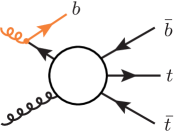
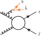
Figure 1: Sample $t\bar{t}b\bar{b}$ diagrams with IS (left) and FS (right) $g\to b\bar{b}$ splittings. In NLOPS simulations of inclusive $t\bar{t}$ production in the 5F scheme the black subtopologies are described in terms of tree matrix elements, while the orange lines correspond to parton shower emissions.

Inclusive NLOPS generators of $t\bar{t}$ production Frixione:2003ei ; Frixione:2007nw are based on $pp\to t\bar{t}$ NLO matrix elements matched to partons showers in the 5F scheme. In this framework, as illustrated in Fig. 1, $t\bar{t}+b$-jet events are generated starting from $2\to 3$ tree matrix elements of type $gb\to t\bar{t}b$ or $gg/q\bar{q}\to t\bar{t}g$. In the latter case, $t\bar{t}b\bar{b}$ events arise via FS $g\to b\bar{b}$ shower splittings. Instead, in the case of $gb\to t\bar{t}b$ the final-state $b$-quark emerges from the matrix element, while $g\to b\bar{b}$ splittings generate the initial-state $b$-quark through the evolution of the 5F PDFs. The unresolved spectator $b$-quark associated with such IS $g\to b\bar{b}$ splittings is emitted by the parton shower via backward evolution. The main advantage of the 5F scheme lies in the resummation of potentially large $\alpha_{\rm S}\ln(m_{t}/m_{b})$ terms associated with the evolution of the $b$-quark density. However, such logarithmic effects are typically rather mild at the LHC Maltoni:2012pa . Moreover, as we will show in Section 2.3, $t\bar{t}+b$-jet production is largely dominated by topologies with FS $g\to b\bar{b}$ splittings. For this reason, $t\bar{t}+b$-jet predictions based on NLOPS $t\bar{t}$ generators suffer from the twofold disadvantage given by the direct dependence on the parton-shower modelling of FS $g\to b\bar{b}$ splittings plus the LO nature of the underlying $t\bar{t}g$ matrix element.

2.2 $\boldsymbol{t\bar{t}+}$multi-jet merging in the five-flavour scheme

As a possible strategy to reduce the sensitivity to the parton shower and increase the accuracy of theoretical predictions we consider $t\bar{t}+$multi-jet merging in the 5F scheme. In this approach, a tower of NLOPS simulations for $t\bar{t}+0,1,\dots,N$ jet production is merged into a single inclusive sample Hoeche:2012yf ; Lonnblad:2012ix ; Frederix:2012ps . This is achieved by clustering QCD partons into jets with a certain $k_{\mathrm{T}}$-resolution, $Q_{\mathrm{cut}}$, which is known as merging scale. At LO, the phase-space regions with $N=0,1,\dots,N_{\mathrm{max}}$ resolved jets ($k_{T}>Q_{\mathrm{cut}}$) are described in terms of $t\bar{t}+N$-jet LOPS simulations. The LOPS simulation with $N_{\mathrm{max}}$ jets fills also the phase space with $N>N_{\mathrm{max}}$ resolved jets by means of the parton shower. At NLO, the resolution criterion used to separate regions of different jet multiplicity exactly the same as for LO, while the basic difference with respect to LO merging lies in the fact that $t\bar{t}+N$-jet LOPS simulations are replaced by corresponding NLOPS simulations. Thus in NLO (LO) merging the effective number of resolved jets that is described at NLOPS (LOPS) accuracy is $N_{\mathrm{eff}}=\mathrm{min}\{N,N_{\mathrm{\max}}\}$, while the $(N_{\mathrm{eff}}+1)^{\mathrm{th}}$ resolved or unresolved jet is described at LOPS (pure PS) accuracy, and all remaining resolved or unresolved jets are described at pure PS accuracy.

Multi-jet merging for $t\bar{t}+$jet at NLO can be performed in a fully automated way within the Sherpa Gleisberg:2008ta and Madgraph5aMC@NLO Alwall:2014hca frameworks. However, the fact that $t\bar{t}+b$-jet events constitute only a small fraction of a $t\bar{t}+$jets sample poses very high requirements in terms of Monte Carlo statistics. Moreover, in order to minimise the dependence on parton-shower modelling, such simulations should be performed using a small merging scale and including a sufficiently high number of NLO jets, $N_{\mathrm{max}}$. The required CPU resources grow very fast at large $N_{\mathrm{max}}$ and small $Q_{\mathrm{cut}}$, and state-of-the-art merged simulations can handle up to two jets at NLO Hoeche:2014qda at present.

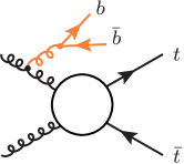
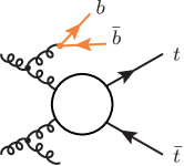
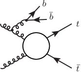
Figure 2: Sample diagrams describing the interplay between matrix elements (black) and parton shower (orange) for $t\bar{t}+b$-jet events in merged LOPS simulations of $t\bar{t}+0,1,2$ jet production in the 5F scheme. In regions where the $b\bar{b}$ system and its parent gluon are produced below the merging scale, the event is described through hard $t\bar{t}$ matrix elements plus parton-shower branchings (a). When the parent gluon becomes harder, the parton shower is used only to model collinear $g\to b\bar{b}$ splittings (b). Above the merging scale, if $g\to b\bar{b}$ splittings do not belong to the two hardest branchings they are still left to the parton shower, while $2\to 4$ matrix elements are used to account for other light jets (c). Otherwise, the event is described through $t\bar{t}b\bar{b}$ matrix elements (d).

The multi-jet merging description of $t\bar{t}b\bar{b}$ events with FS $g\to b\bar{b}$ splittings is sketched in Fig. 2 for the case of $t\bar{t}+0,1,2$-jet merging at LO. In regions where the $b\bar{b}$ pair and/or the parent gluon are emitted at small scales, $g\to b\bar{b}$ splittings are expected to be generated by the parton shower, while hard $b$-jet pairs are expected to arise from $t\bar{t}b\bar{b}$ matrix elements. However, as we will see, typical $t\bar{t}+b$-jet events involve additional light jets that are emitted at harder scales with respect to the $g\to b\bar{b}$ branching. In that case, $2\to 4$ matrix elements account only for light jets, and $g\to b\bar{b}$ splittings are left to the parton shower. In general, the relative importance of matrix elements and parton shower depends on the resolution scale $Q_{\mathrm{cut}}$, and using a finite resolution is mandatory in the 5F scheme, since collinear $g\to b\bar{b}$ splittings are divergent, i.e. $t\bar{t}b\bar{b}$ matrix elements cannot be used in the full phase space.

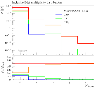
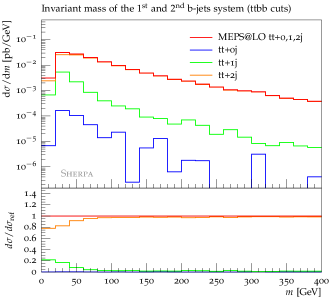
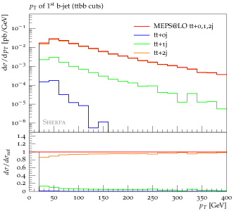
Figure 3: Breakdown of merged LOPS simulations of $pp\to t\bar{t}+0,1,2$ jets production at 13 TeV into the contributions from matrix elements with $t\bar{t}+$0,1 and 2 generic QCD partons: distributions in the number of $b$-jets with $p_{\mathrm{T}}>25$ GeV (a), the invariant mass of the two leading $b$-jets (b), and the $p_{\mathrm{T}}$ of the leading $b$-jet (c).

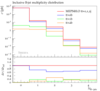
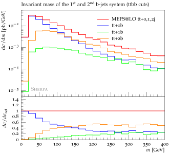
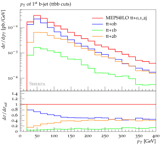
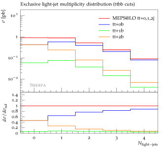
Figure 4: Breakdown of merged LOPS simulations of $t\bar{t}+0,1,2$ jets production at 13 TeV into the contributions from matrix elements with $t\bar{t}+$0,1 and 2 $b$-quarks. Same observables (a)–(c) as in Fig. 3 and distribution in the exclusive number of light jets with $p_{\mathrm{T}}>25$ GeV (d) in the presence of ttbb cuts.

In Figures 3–4 we analyse the matrix-element content of a $t\bar{t}+0,1,2$-jet merged simulation at LO. These studies are based on the MEPS@LO method Hoeche:2009rj implemented in Sherpa, but the main findings are expected to hold also for other merging methods. Besides the $b$-jet multiplicity distribution, in Figures 3–4 we plot differential observables in the presence of ttbb cuts, i.e. requiring $N_{b}\geq 2$ $b$-jets as defined in Section 3.6. For jets we apply the acceptance cuts (39) and, in order to maximise the possibility to resolve jets at matrix-element level, we choose a merging scale lower than the jet-$p_{\mathrm{T}}$ threshold, $Q_{\mathrm{cut}}=20$ GeV.

As expected, in Fig. 3 we find that $t\bar{t}+b$-jet observables with $N_{b}\geq 2$ resolved $b$-jets are largely dominated by $t\bar{t}+$2-parton matrix elements. This holds also for $N_{b}\geq 1$. However, the breakdown of the merged sample into contributions from matrix elements with different $b$-quark multiplicity in Fig. 4 reveals that, in spite of the low merging scale, the cross section for producing one or more $b$-jets is dominated by matrix elements with zero $b$-quarks. The contribution of $t\bar{t}b\bar{b}$ matrix elements hardly exceeds 50% even in the region of large $b$-jet $p_{\mathrm{T}}$ or large invariant mass of the $b$-jet pair. This counterintuitive feature can be attributed to the fact that, in $t\bar{t}+$jet events that involve $g\to b\bar{b}$ splittings, the two hardest QCD branchings are typically associated with the emission of the parent gluon of the $b\bar{b}$ pairs and/or with the production of other light jets. As a consequence, in LOPS merged samples with $N_{\mathrm{max}}=2$, $g\to b\bar{b}$ splittings are left to the parton shower. We have verified that the contribution of $t\bar{t}b\bar{b}$ matrix elements remains relatively low even when the merging procedure is extended up to 3 or 4 jets with $Q_{\mathrm{cut}}=20$ GeV. Moreover, we have checked that increasing the merging scale leads to a further suppression of the contribution of $t\bar{t}b\bar{b}$ matrix elements.

Fig. 4d demonstrates that $t\bar{t}+2\,b$-jet events are indeed accompanied by abundant emission of extra light jets, and the importance of $t\bar{t}b\bar{b}$ matrix elements decreases with increasing light-jets multiplicity. Moreover, even in the bin with zero additional light jets it turns out that the contribution of $t\bar{t}b\bar{b}$ matrix elements remains below 50%. This is probably due to the fact that $g\to b\bar{b}$ splittings tend to take place at branching scales below the jet-$p_{\mathrm{T}}$-threshold of 25 GeV.

In summary, contrary to naive expectations, $t\bar{t}+$jets samples based on LOPS merging do not guarantee a matrix-element description of $b$-jet production but largely rely on the parton shower modelling of $g\to b\bar{b}$ splittings. In the case of multi-jet merging at NLO, to a certain extent $g\to b\bar{b}$ shower splittings should be matched to $t\bar{t}b\bar{b}$ and $t\bar{t}b\bar{b}g$ tree matrix elements. Nevertheless, based on the above observations, the theoretical accuracy in the description of $b$-jet production is expected to remain between the LOPS and the pure PS level. Finally, in the light of the presence of abundant light-jet radiation with a typical hardness beyond the one of $b$-jets, the role of hard radiation on top of the $t\bar{t}b\bar{b}$ system should be studied with great care also in the context of NLOPS simulations of $t\bar{t}b\bar{b}$ production (see Section 3.1).

2.3 $\boldsymbol{t\bar{t}b\bar{b}}$ production in the four-flavour scheme

In order to minimise the dependence on parton-shower modelling and to maximise the use of higher-order matrix elements, in the following we will adopt a description of $t\bar{t}+b$-jet production based on $ttbb$ matrix elements in the 4F scheme. In this scheme, $b$-quarks are treated as massive partons, and $g\to b\bar{b}$ splittings are free from collinear singularities. Thus $t\bar{t}b\bar{b}$ matrix elements can be used in the entire phase space. Generic $t\bar{t}b\bar{b}$ topologies where $b$-quarks emerge from IS and FS splitting processes are illustrated in Fig. 5. In the case of FS $g\to b\bar{b}$ splittings, $t\bar{t}b\bar{b}$ matrix elements with $m_{b}>0$ can be extended to the collinear regime, where the $b\bar{b}$ pair becomes unresolved within a single $b$-jet. Similarly, 4F $t\bar{t}b\bar{b}$ matrix elements describe also collinear IS $g\to b\bar{b}$ splittings, where the spectator $b$-quark is emitted in the beam direction and remains unresolved, while the $bg\to t\bar{t}b$ sub-process with a single $b$-jet corresponds to the description of $t\bar{t}+b$-jet production at LO in the 5F scheme. Thus, $t\bar{t}b\bar{b}$ matrix elements provide a fully inclusive description of $t\bar{t}+b$-jet production, and NLO predictions in the 4F scheme yield NLO accuracy both for observables with two $b$-jets and for more inclusive observables with a single resolved $b$-jet.

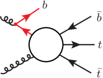
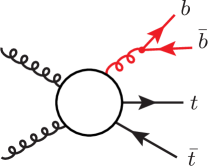
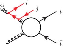
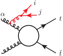
Figure 5: Generic leading-order $gg\to t\bar{t}b\bar{b}$ topologies. The first line shows the most general form of topologies with IS (a) and FS (b) $g\to b\bar{b}$ splittings. The second line shows the generic form of those topologies with IS (c) and FS (d) splittings that turn out to dominate $gg\to t\bar{t}b\bar{b}$. The labels $ij=56,65$ stand for the $b\bar{b}$ system, while $\alpha=1,2$ indicates the initial-state gluon that generates the radiation.

The inclusion of $m_{b}$ effects in $g\to b\bar{b}$ splittings represents a clear advantage of the 4F scheme with respect to the 5F scheme. However, the 4F scheme has the disadvantage that potentially large $\alpha_{\rm S}\ln(m_{b}/Q)$ terms that arise from IS $g\to b\bar{b}$ splittings are not resummed through the PDF evolution. In the following, in order to assess the relevance of this limitation, we decompose the $pp\to t\bar{t}b\bar{b}$ LO cross section into contributions from IS and FS $g\to b\bar{b}$ splittings. Since the $q\bar{q}$ channel involves only FS $g\to b\bar{b}$ splitting, we focus on the $gg$ channel and we first consider a naive diagrammatic splitting of the $gg\to t\bar{t}b\bar{b}$ matrix element,

$$\mathcal{M}_{t\bar{t}b\bar{b}}=\mathcal{M}_{\mathrm{IS},t\bar{t}b\bar{b}}+\mathcal{M}_{\mathrm{FS},t\bar{t}b\bar{b}}+\mathcal{M}_{\mathrm{rem},t\bar{t}b\bar{b}}.$$ (1)

The terms $\mathcal{M}_{\mathrm{IS},t\bar{t}b\bar{b}}$ and $\mathcal{M}_{\mathrm{FS},t\bar{t}b\bar{b}}$ correspond, respectively, to 18 diagrams with IS $g\to b\bar{b}$ splittings and 16 diagrams with FS $g\to b\bar{b}$ splittings. Generic diagrams with IS and FS splittings are depicted in Fig. 5a–b. The term $\mathcal{M}_{\mathrm{rem},t\bar{t}b\bar{b}}$ corresponds to two remaining diagrams where an $s$-channel gluon splits into an on-shell $b$-quark and an off-shell $b$-line coupled to the $t\bar{t}$ system. Its numerical impact turns out to be negligible. Based on (1) we split the $t\bar{t}b\bar{b}$ cross section into three terms,

$$\mathrm{d}\sigma_{t\bar{t}b\bar{b}}=\mathrm{d}\sigma_{\mathrm{IS},t\bar{t}b\bar{b}}+\mathrm{d}\sigma_{\mathrm{FS},t\bar{t}b\bar{b}}+\mathrm{d}\sigma_{\mathrm{int},t\bar{t}b\bar{b}},$$ (2)

where the IS and FS parts are defined as

$$\mathrm{d}\sigma_{\mathrm{IS},t\bar{t}b\bar{b}}=\frac{|\mathcal{M}_{\mathrm{IS},t\bar{t}b\bar{b}}|^{2}}{|\mathcal{M}_{t\bar{t}b\bar{b}}|^{2}}\,\mathrm{d}\sigma_{t\bar{t}b\bar{b}},\qquad\mathrm{d}\sigma_{\mathrm{FS},t\bar{t}b\bar{b}}=\frac{|\mathcal{M}_{\mathrm{FS},t\bar{t}b\bar{b}}|^{2}}{|\mathcal{M}_{t\bar{t}b\bar{b}}|^{2}}\,\mathrm{d}\sigma_{t\bar{t}b\bar{b}},$$ (3)

while $\mathrm{d}\sigma_{\mathrm{int},t\bar{t}b\bar{b}}$ consists of the interference between $\mathcal{M}_{\mathrm{IS},t\bar{t}b\bar{b}}$ and $\mathcal{M}_{\mathrm{FS},t\bar{t}b\bar{b}}$ plus a minor contribution from $\mathcal{M}_{\mathrm{rem},t\bar{t}b\bar{b}}$.

In order to check the soundness of the above gauge-dependent separation we compare it to an alternative definition of IS and FS $g\to b\bar{b}$ contributions based on the collinear limits of the $gg\to t\bar{t}b\bar{b}$ matrix element. In this case we define

$$\mathrm{d}\sigma_{\mathrm{IS}\otimes t\bar{t}}=\frac{|\mathcal{M}_{\mathrm{IS}\otimes t\bar{t}}|^{2}}{|\mathcal{M}_{t\bar{t}b\bar{b}}|^{2}}\,\mathrm{d}\sigma_{t\bar{t}b\bar{b}},\qquad\mathrm{d}\sigma_{\mathrm{FS}\otimes t\bar{t}}=\frac{|\mathcal{M}_{\mathrm{FS}\otimes t\bar{t}}|^{2}}{|\mathcal{M}_{t\bar{t}b\bar{b}}|^{2}}\,\mathrm{d}\sigma_{t\bar{t}b\bar{b}}.$$ (4)

Here $|\mathcal{M}_{\mathrm{IS}\otimes t\bar{t}}|^{2}$ and $|\mathcal{M}_{\mathrm{FS}\otimes t\bar{t}}|^{2}$ describe the collinear limits of the topologies depicted in Fig. 5c and 5d, respectively. Note that, for simplicity, we consider only the leading collinear enhancements where the $b\bar{b}$ system originates either through the combination of $g\to b\bar{b}$ and $b\to gb$ IS splittings ($\mathcal{M}_{\mathrm{IS}\otimes t\bar{t}}$) or via IS $g\to gg$ plus FS $g\to b\bar{b}$ splittings ($\mathcal{M}_{\mathrm{FS}\otimes t\bar{t}}$). For events with external momenta

$$g(p_{1})\,g(p_{2})\to t(p_{3})\,\bar{t}(p_{4})\,b(p_{5})\,\bar{b}(p_{6}),$$ (5)

the collinear limits take the general form

$$\big{|}\mathcal{M}_{\mathrm{IS}\otimes t\bar{t}/\mathrm{FS}\otimes t\bar{t}}\big{|}^{2} = (8\pi\alpha_{\rm S})^{2}\,\max_{\alpha=1,2\atop ij=56,65}\left\{\frac{K_{\mathrm{IS}/\mathrm{FS}}(p_{\alpha},p_{i},p_{j})}{(p_{\alpha}-p_{i}-p_{j})^{2}}\,\big{|}\mathcal{M}_{gg\to t\bar{t}}\big{|}^{2}_{p_{\alpha}\to zp_{\alpha}}\right\},$$ (6)

where $\alpha\in\{1,2\}$ and $ij\in\{56,65\}$ specify, respectively, the IS gluon emitter and the ordering of the $b\bar{b}$ pair as depicted in Fig. 5c and 5d. $K_{\mathrm{IS}/\mathrm{FS}}(p_{\alpha},p_{i},p_{j})$ are the corresponding splitting kernels. The choice of $\alpha$ and $ij$ specifies a particular topology, and the maximum in (6) defines $\big{|}\mathcal{M}_{\mathrm{IS}\otimes t\bar{t}}\big{|}^{2}$ and $\big{|}\mathcal{M}_{\mathrm{FS}\otimes t\bar{t}}\big{|}^{2}$ as the collinear limit of the most likely topology of IS and FS type. The splitting kernels read

$$K_{\mathrm{IS}}(p_{\alpha},p_{i},p_{j}) = \frac{1}{(p_{\alpha}-p_{i})^{2}-m_{b}^{2}}\frac{P_{gq}(x_{\mathrm{IS}})}{x_{\mathrm{IS}}}\frac{P_{qg}(y_{\mathrm{IS}})}{y_{\mathrm{IS}}},$$

$$K_{\mathrm{FS}}(p_{\alpha},p_{i},p_{j}) = \frac{-1}{(p_{i}+p_{j})^{2}}\frac{P_{gg}(z)}{z}P_{gq}(x_{\mathrm{FS}}),$$ (7)

where

$$P_{gq}(x) =T_{R}\left[1-2x(1-x)\right], P_{qg}(x) =C_{F}\left[\frac{1+(1-x)^{2}}{x}\right],$$

$$P_{gg}(x) =2C_{A}\left[\frac{x}{1-x}+\frac{1-x}{x}+x(1-x)\right],$$ (8)

with $T_{R}=1/2$, $C_{F}=4/3$ and $C_{A}=3$. The various momentum fractions are set to

$$x_{\mathrm{IS}} =\frac{E_{\alpha}-E_{i}}{E_{\alpha}} y_{\mathrm{IS}} =\frac{E_{\alpha}-(E_{i}+E_{j})}{E_{\alpha}-E_{i}},$$

$$x_{\mathrm{FS}} =\frac{E_{j}}{E_{i}+E_{j}}, z =x_{\mathrm{IS}}\,y_{\mathrm{IS}}\,.$$ (9)

Finally, the underlying $gg\to t\bar{t}$ squared matrix element in (6) reads

$$\big{|}\mathcal{M}_{gg\to t\bar{t}}\big{|}^{2}_{p_{\alpha}\to zp_{\alpha}} = \left(4\pi\alpha_{\rm S}\right)^{2}\theta\left(z-\frac{m_{t\bar{t}}}{p_{1}\cdot p_{2}}\right)\Bigg{\{}\left[\frac{(p_{1}\cdot p_{2})^{2}}{6(p_{1}\cdot p_{3})(p_{2}\cdot p_{3})}-\frac{3}{8}\right]$$ (10)

$$\times \left[\frac{(p_{1}\cdot p_{3})^{2}}{(p_{1}\cdot p_{2})^{2}}+\frac{(p_{2}\cdot p_{3})^{2}}{(p_{1}\cdot p_{2})^{2}}-\frac{2m_{t}^{2}}{(p_{1}\cdot p_{2})}+\frac{m_{t}^{4}}{(p_{1}\cdot p_{3})(p_{2}\cdot p_{3})}\right]\bigg{\}}_{p_{\alpha}\to zp_{\alpha}},\hskip 11.38109pt$$

where helicity/colour sums and average factors are included, and the momentum of the IS emitter has to be rescaled by $z$.

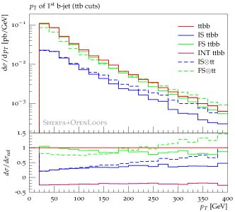
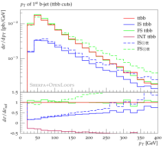
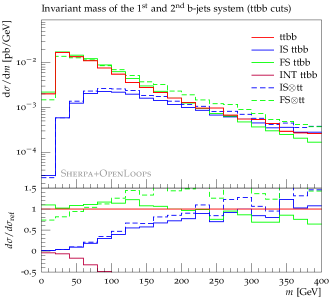
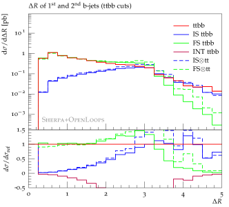
Figure 6: Breakdown of the $pp\to t\bar{t}b\bar{b}$ cross section into contributions from topologies with IS and FS splittings at fixed-order LO in the 4F scheme: distributions in the $p_{\mathrm{T}}$ of the leading $b$-jet with ttb (a) and ttbb (b) cuts, and distributions in the invariant mass (c) and $\Delta R$ separation (d) of the two leading $b$-jets with ttbb cuts. The complete $gg/q\bar{q}\to t\bar{t}b\bar{b}$ matrix-element prediction (solid red) is split according to (2) into contributions from topologies of IS (solid blue) and FS (solid green) type and their interference (solid purple). This is compared to the gauge-invariant breakdown (4) into IS (dashed blue) and FS (dashed green) parts based on the collinear limits of the $t\bar{t}b\bar{b}$ matrix element. Note that the $q\bar{q}$ channel consists solely of FS $g\to b\bar{b}$ contributions.

Numerical results for the diagrammatic decomposition (2) and the collinear decomposition (4) of $pp\to t\bar{t}b\bar{b}$ at $\sqrt{s}=13$ TeV are shown in Fig. 6. The first two plots display the leading $b$-jet $p_{\mathrm{T}}$ distribution in the presence of ttb and ttbb cuts as defined in Section 3.6, i.e. requiring $N_{b}\geq 1$ and $N_{b}\geq 2$ $b$-jets, respectively. In the ttbb phase space, topologies with $g\to b\bar{b}$ FS splittings turn out to be surprisingly close to the full matrix element, with deviations that do not exceed the 10% level in the entire spectrum. This agreement remains remarkably good also in the inclusive ttb phase space, where IS splitting processes with one unresolved $b$-quark are expected to be more pronounced. Actually, with ttb and ttbb cuts the pure IS contribution ranges between 20–40% and 15–75%, respectively, but is almost entirely cancelled by the IS–FS interference.

The fact that the collinear approximations (4) agree rather well with the corresponding squared Feynman diagrams up to relatively high $p_{\mathrm{T}}$ confirms that $t\bar{t}b\bar{b}$ production is dominated by the topologies in Fig. 5c and 5d. On the other hand, the importance of interference effects provides strong motivation for using exact $t\bar{t}b\bar{b}$ matrix elements, while collinear approximations such as those in (6) or in the parton-shower modelling of $g\to b\bar{b}$ splittings should be used with due caution.

The above considerations apply also for the $m_{b\bar{b}}$ and $\Delta R_{b\bar{b}}$ distribution in Fig. 6c and d. In particular, we observe that topologies with FS $g\to b\bar{b}$ splittings are very close to the full matrix element in the whole $m_{b\bar{b}}$ spectrum as well as for $\Delta R_{b\bar{b}}<2$ . At the same time, for $50\,\text{GeV}<m_{b\bar{b}}<200\,\text{GeV}$ and $1<\Delta R_{b\bar{b}}<2.5$, i.e. in the range of interest for $t\bar{t}H(b\bar{b})$ analyses, we observe that IS splitting contributions and negative interference effects grow fast and tend to become very sizable. Thus a naive separation into contributions from IS and FS splittings is not applicable at large $m_{b\bar{b}}$ and $\Delta R_{b\bar{b}}$. On the other hand, in the region of moderate invariant mass and $\Delta R$ separation, which contains the bulk of the $t\bar{t}b\bar{b}$ cross section, interference effects are rather small, and $b\bar{b}$ pairs turn out to originate almost entirely from FS $g\to b\bar{b}$ splittings.

In summary, given that the 5F scheme is based on the LO process $gb\to t\bar{t}b$, where FS $g\to b\bar{b}$ splittings and interference effects are entirely neglected, the above observations provide strong motivation for a description of $t\bar{t}+b$-jet production based on $t\bar{t}b\bar{b}$ matrix elements in the 4F scheme.

3 Technical aspects and setup of NLOPS $\boldsymbol{t\bar{t}b\bar{b}}$ simulations

In this section we introduce a new Powheg generator based on $t\bar{t}b\bar{b}$ matrix elements in the 4F scheme. Special emphasis is devoted to some technical aspects of the Powheg method that turn out to play an important role for multi-scale processes like $pp\to t\bar{t}b\bar{b}$. In addition we describe the setup used for the $t\bar{t}+b$-jet simulations presented in Sections 4–5, i.e. all relevant input parameters, scale choices and parton shower settings, as well as the treatment of theoretical uncertainties and the definitions of physics objects and selection cuts. Finally we provide details on the treatment of top-quark decays.

The new $t\bar{t}b\bar{b}$ generator is implemented in the Powheg-Box-Res framework Jezo:2015aia , and the relevant LO and NLO matrix elements are computed by OpenLoops Cascioli:2011va ; OLhepforge ; Buccioni:2017yxi through its Powheg-Box-Res interface Jezo:2016ujg . For the evaluation of one-loop integrals OpenLoops employs the Collier library Denner:2014gla ; Denner:2002ii ; Denner:2005nn ; Denner:2010tr and, alternatively, CutTools Ossola:2007ax ; Ossola:2006us together with the OneLOop library vanHameren:2010cp . While we do not apply the resonance-aware method Jezo:2015aia , the Powheg-Box-Res framework allows us to make use of new technical features, such as the automated implementation of scale variations , a Rivet Buckley:2010ar interface and the option to unweight events partially. This $t\bar{t}b\bar{b}$ generator will be soon publicly available on the Powheg-Box webpage PWGBpage .

3.1 Powheg methodology

In the following, we briefly review the Powheg method Nason:2004rx ; Frixione:2007vw with emphasis on the separation of radiation into singular and finite parts. In this context we discuss technical subtleties that arise in the case of multi-scale processes like $pp\to t\bar{t}b\bar{b}$.

The master formula for the description of NLO radiation in the Powheg approach consists of two contributions,

$$\mathrm{d}\sigma = \mathrm{d}\sigma_{\mathrm{s}}+\mathrm{d}\sigma_{\mathrm{f}},$$ (11)

which arise from the splitting of real emission into singular (s) and finite (f) parts,

$$R(\Phi_{\mathrm{R}})=R_{\mathrm{s}}(\Phi_{\mathrm{R}})+R_{\mathrm{f}}(\Phi_{\mathrm{R}}).$$ (12)

Here $R(\Phi_{\mathrm{R}})$ should be understood as squared real-emission matrix element, and $\Phi_{\mathrm{R}}$ as the corresponding phase space. Similarly, Born and virtual contributions in the Born phase space are denoted as $B(\Phi_{\mathrm{B}})$ and $V(\Phi_{\mathrm{B}})$. The splitting (12) is implemented as

$$R_{\mathrm{s}}(\Phi_{\mathrm{R}})=F(\Phi_{\mathrm{R}})\,R(\Phi_{\mathrm{R}}),\qquad R_{\mathrm{f}}(\Phi_{\mathrm{R}})=\left[1-F(\Phi_{\mathrm{R}})\right]\,R(\Phi_{\mathrm{R}}),\qquad$$ (13)

where $F(\Phi_{\mathrm{R}})\in[0,1]$ is a damping function that fulfils $F\to 1$ and $F\to 0$, respectively, in the infrared and hard regions of phase space (see below).

The singular part of real radiation is resummed according to the Powheg formula

$$\mathrm{d}\sigma_{\mathrm{s}} = \bar{B}(\Phi_{\mathrm{B}})\,\mathrm{d}\Phi_{\mathrm{B}}\left[\Delta(q_{\operatorname{cut}})+\sum_{\alpha}\Delta(k_{\mathrm{T},\alpha})\frac{R_{\mathrm{s},\alpha}(\Phi_{\alpha}(\Phi_{\mathrm{B}},\Phi_{\operatorname{rad}}))}{B(\Phi_{\mathrm{B}})}\,\mathrm{d}\Phi_{\operatorname{rad}}\right],$$ (14)

where real emission is further split into FKS sectors Frixione:1995ms ,

$$R_{\mathrm{s}}=\sum_{\alpha}R_{\mathrm{s},\alpha},\qquad R_{\mathrm{f}}=\sum_{\alpha}R_{\mathrm{f},\alpha},$$ (15)

which isolate collinear singularities arising from individual emitters. In each sector, the emission phase space $\Phi_{\mathrm{R}}$ is factorised into the Born phase space $\Phi_{\mathrm{B}}$ and a one-particle radiation phase space $\Phi_{\operatorname{rad}}$ through an appropriate FKS mapping,

$$(\Phi_{\mathrm{B}},\Phi_{\operatorname{rad}})\;\longrightarrow\;\Phi_{\mathrm{R}}=\Phi_{\alpha}(\Phi_{\mathrm{B}},\Phi_{\operatorname{rad}}).$$ (16)

The term within squared brackets in (14) generates the hardest radiation according to an emission probability $R/B$. The parameter $k_{\mathrm{T},\alpha}=k_{\mathrm{T},\alpha}(\Phi_{\mathrm{rad}})$ stands for the hardness of the radiated parton, and radiation harder than $k_{\mathrm{T},\alpha}$ is excluded by means of corresponding Sudakov form factors,

$$\Delta(q) = \exp\left[-\sum_{\alpha}\,\int_{k_{\mathrm{T},\alpha}\,>\,q}\frac{R_{\mathrm{s},\alpha}(\Phi_{\alpha}(\Phi_{\mathrm{B}},\Phi_{\operatorname{rad}}))}{B(\Phi_{\mathrm{B}})}\,\mathrm{d}\Phi_{\operatorname{rad}}\right].$$ (17)

The term $\Delta(q_{\operatorname{cut}})$ in (14) represents the no-emission probability above the infrared cutoff $q_{\operatorname{cut}}$, and Sudakov form factors account for unresolved multiple emissions in a way that cancels infrared singularities while preserving the differential NLO cross section $\bar{B}(\Phi_{\mathrm{B}})$ in the Born phase space. The latter is defined by integrating out the singular part of real radiation,

$$\bar{B}(\Phi_{\mathrm{B}}) = B(\Phi_{\mathrm{B}})+V(\Phi_{\mathrm{B}})+\sum_{\alpha}\int R_{\mathrm{s},\alpha}(\Phi_{\alpha}(\Phi_{\mathrm{B}}\,,\Phi_{\operatorname{rad}}))\,\mathrm{d}\Phi_{\operatorname{rad}}\,.$$ (18)

Here infrared cancellations between $V$ and $R_{\mathrm{s}}$ are controlled via FKS subtraction. The remaining finite part of NLO radiation is treated as in fixed-order calculations,

$$\mathrm{d}\sigma_{\mathrm{f}} = \sum_{\alpha}R_{\mathrm{f},\alpha}(\Phi_{\alpha}(\Phi_{\mathrm{B}},\Phi_{\operatorname{rad}}))\,\mathrm{d}\Phi_{\mathrm{B}},\mathrm{d}\Phi_{\operatorname{rad}}\,.$$ (19)

Note that flux and symmetry factors as well as the convolution with PDFs are implicitly understood in (14) and (19).

Let us now come back to the details of the separation of the singular and finite parts of real emission in (13). Technically, the damping function $F$ is implemented based on the kinematics of the actual FKS sector, i.e.

$$R_{\mathrm{s},\alpha}(\Phi_{\alpha})=R_{\alpha}(\Phi_{\alpha})-R_{\mathrm{f},\alpha}(\Phi_{\alpha})=F_{\alpha}(\Phi_{\alpha})R_{\alpha}(\Phi_{\alpha}).$$ (20)

The default functional form of $F$ in Powheg-Box Alioli:2010xd ; Alioli:2008tz is

$$F_{\alpha}(\Phi_{\alpha})=F_{\mathrm{damp},\alpha}(\Phi_{\alpha})\,F_{\mathrm{bzd},\alpha}(\Phi_{\alpha}),$$ (21)

where

$$F_{\mathrm{damp},\alpha}(\Phi_{\alpha})=\frac{h_{\mathrm{damp}}^{2}}{h_{\mathrm{damp}}^{2}+k_{\mathrm{T},\alpha}^{2}}$$ (22)

is the usual factor that smoothly shifts the weight of real radiation from $R_{\mathrm{s}}$ to $R_{\mathrm{f}}$ when the hardness of the emission, $k_{\mathrm{T},\alpha}$, becomes of the order of $h_{\mathrm{damp}}$ or higher. Note that the freely adjustable $h_{\mathrm{damp}}$ parameter in Powheg plays an analogous role as the resummation scale $\mu_{Q}$ in the MC@NLO method. This is because both parameters act as a $k_{\mathrm{T}}$-threshold that separates the radiative phase space into a hard region, which is described by fixed-order matrix elements, from a singular region, where large logarithms of soft and collinear origin are resummed to all orders by means of Sudakov form factors. More precisely, in the MC@NLO approach the factor $R_{\mathrm{s},\alpha}/B$ and the terms $\Delta$ in (14) correspond, respectively, to the parton-shower emission probability and the associated Sudakov form factors. Thus, in the MC@NLO framework, equation (14) corresponds to the weight of so-called soft events supplemented by the probability of the first parton-shower emission and its no-emission counterpart. In analogy with (21)–(22), also the first MC@NLO shower emission is modulated by a certain damping function. The related reference scale $\mu_{Q}$, i.e. the MC@NLO counterpart of the scale $h_{\mathrm{damp}}$ in Powheg, corresponds to the upper bound of the first shower emission in MC@NLO. Thus MC@NLO predictions are sensitive to the choice of the shower starting scale. On the contrary, the first Powheg emission in (11)–(13) is entirely determined by the matrix element, which also dictates the scale at which the shower starts emitting further partons. Thus the Powheg method has the advantage of being essentially independent on the shower starting scale. More generally, thanks to the fact that the first emission is completely independent of the parton shower, Powheg predictions are characterised by a rather mild sensitivity to systematic uncertainties associated with the parton shower.

In addition to the well-known $h_{\mathrm{damp}}$-dependent damping mechanism (22), the Powheg-Box also implements a theta function of the form Alioli:2008gx ; Alioli:2010xd

$$F_{\mathrm{bzd},\alpha}(\Phi_{\alpha})=\theta\left(h_{\mathrm{bzd}}-\frac{R_{\alpha}(\Phi_{\alpha})}{\mathcal{R}_{\alpha}(\Phi_{\alpha})}\right),$$ (23)

where $\mathcal{R}_{\alpha}$ corresponds to the infrared (soft and collinear) approximation of the full matrix element. Schematically it has the factorised form

$$\mathcal{R}_{\alpha}(\Phi_{\alpha})=\mathcal{K}_{\alpha}(\Phi_{\mathrm{rad}})B(\Phi_{\mathrm{B}}),$$ (24)

with an FKS kernel $\mathcal{K}_{\alpha}(\Phi_{\mathrm{rad}})$ and an underlying Born contribution $B(\Phi_{\mathrm{B}})$, whose kinematics is determined by the inverse of the mapping (16) in the actual sector $\alpha$. By default, the cut-off parameter $h_{\mathrm{bzd}}$ in (23) is set equal to 5. In this way, in the vicinity of IR singularities, where $R_{\alpha}/\mathcal{R}_{\alpha}\to 1$, radiative contributions are attributed to $R_{\mathrm{s}}$ and resummed according to (14). On the contrary, when the real emission matrix element largely exceeds the IR approximation (24), the resummation of the full $R/B$ kernel according to (14) is not well justified, and corresponding events are attributed to the finite remnant (19) through the theta function (23). In the standard Powheg-Box, and in Ref. Bevilacqua:2017cru , the damping function (21) is applied only to initial-state radiation. However, in the present $t\bar{t}b\bar{b}$ generator we have extended it to all (massless or massive) final-state emitters, that have a FKS sector associated with it, in order to ensure a consistent resummation of QCD radiation off $b$-quarks.

The requirement $R_{\alpha}(\Phi_{\alpha})<h_{\mathrm{bzd}}\,\mathcal{K}_{\alpha}(\Phi_{\mathrm{rad}})\,B(\Phi_{\mathrm{B}})$ was originally introduced in order to avoid possible divergences of $R(\Phi_{\alpha})/B(\Phi_{\mathrm{B}})$ due to so-called Born zeros, i.e. phase space regions where $B(\Phi_{\mathrm{B}})\to 0$. Such divergences cancel in the $\bar{B}/B$ ratio, i.e. they are not physical, and are not related to IR radiation. Corresponding $\Phi_{\mathrm{B}}$ regions should thus be attributed to the finite remnant. Otherwise they could lead to dramatic inefficiencies in the event generation. More generally, the damping factor (23) can play an important role also in case of multi-scale processes where the Born cross section involves enhancement mechanisms at scales well below the hard energy of the full process. Such enhancements can compete with the ones due to soft and collinear QCD radiation in a way that is somewhat analogous to Born zeros.

In the case of $pp\to t\bar{t}b\bar{b}$, such effects can arise from the interplay of soft and collinear enhancements due to NLO light-jet radiation and to the generation of the $b\bar{b}$ system in regions with $m_{b\bar{b}}\ll m_{t\bar{t}b\bar{b}}$ and/or $p_{\mathrm{T},b\bar{b}}\ll m_{t\bar{t}b\bar{b}}$. For example, let us consider a $gg\to t\bar{t}b\bar{b}g$ event with a gluon emission of ISR type. Its kinematics is generated starting from a $gg\to t\bar{t}b\bar{b}$ Born event through a mapping of type (16), which creates the required gluon recoil by boosting the final state of the $gg\to t\bar{t}b\bar{b}$ Born event in the transverse direction. The relevant boost factor, $\gamma=1/(1-\beta^{2})^{1/2}$, is determined by $p_{\mathrm{T},j}=p^{\prime}_{\mathrm{T},t\bar{t}b\bar{b}}=\gamma\beta E_{t\bar{t}b\bar{b}}$, where $E_{t\bar{t}b\bar{b}}$ is the $t\bar{t}b\bar{b}$ energy of the $b\bar{b}$ system in the Born event. If we assume, for simplicity, that he gluon is emitted in the same azimuthal direction as the $b\bar{b}$ system in the Born event, then the $b\bar{b}$ transverse momentum of the radiative event becomes $p^{\prime}_{\mathrm{T},b\bar{b}}=\gamma(p_{\mathrm{T},b\bar{b}}-\beta E_{b\bar{b}})$, where $p_{\mathrm{T},b\bar{b}}$ and $E_{b\bar{b}}$ are the $b\bar{b}$ transverse momentum and energy in the Born event. Thus, the FKS mapping can lead to a very significant reduction of $p_{\mathrm{T},b\bar{b}}$. More precisely, for radiative events with

$$\frac{p_{\mathrm{T},j}}{p_{\mathrm{T},b\bar{b}}}=(1+\epsilon)\frac{E_{t\bar{t}b\bar{b}}}{E_{b\bar{b}}},$$ (25)

the effect of the FKS boost on the $b\bar{b}$ system amounts to

$$\frac{p^{\prime}_{\mathrm{T},b\bar{b}}}{p_{\mathrm{T},b\bar{b}}}=\tilde{\epsilon}=\gamma-1-\epsilon.$$ (26)

Thus, since the bulk of the $t\bar{t}b\bar{b}$ cross section is characterised by $E_{t\bar{t}b\bar{b}}\gg E_{b\bar{b}}$ and $\gamma\sim 1$, in the case of hard QCD radiation with $\tilde{\epsilon}\ll 1$ the FKS mapping can lead to a drastic reduction of the $p_{\mathrm{T}}$ of the $b\bar{b}$ system. As a result, in the region of small $m_{b\bar{b}}$, the ISR boost can enhance the $R_{\alpha}(\Phi_{\alpha})/\mathcal{R}_{\alpha}(\Phi_{\alpha})$ ratio by up to a factor $(p_{\mathrm{T},b\bar{b}}/p^{\prime}_{\mathrm{T},b\bar{b}})^{2}\sim 1/{\tilde{\epsilon}}^{2}$. This violates the main assumption that justifies the Powheg formula (14), namely $R_{\alpha}(\Phi_{\alpha})/B(\Phi_{B})\sim\mathcal{R}_{\alpha}(\Phi_{\alpha})/B(\Phi_{B})={\cal K}_{\alpha}(\Phi_{\mathrm{rad}})$, which requires a sufficiently hard $t\bar{t}b\bar{b}$ process as compared to the $k_{\mathrm{T}}$ of NLO radiation. In particular, due to the sensitivity of the Born amplitude to scales of the order ${p_{\mathrm{T},b\bar{b}}}\sim(E_{b\bar{b}}/E_{t\bar{t}b\bar{b}})\,p_{\mathrm{T},j}\ll p_{\mathrm{T},j}$, the factorisation formula (24) is not fulfilled.

Fortunately, this problematic behaviour emerges only in relatively hard regions of the $\Phi_{\mathrm{rad}}$ phase space. Thus, as a remedy it is natural to shift such events into the finite remnant by means of the damping factor (23). In fact, in the case of $t\bar{t}b\bar{b}$ production we have found that the $h_{\mathrm{bzd}}$-dependent cut plays an important role for the efficiency generation of Les Houches events (LHEs) as well as for a consistent scale dependence. Moreover, applying a large $h_{\mathrm{bzd}}$ cut we have observed a significant enhancement of the QCD scale dependence. This can be attributed to the fact that scale variations in the soft term (14) are restricted to the $\bar{B}$ factor (18), where the unphysical distortions of the $b\bar{b}$ kinematics induced by the FKS mappings can jeopardise the natural cancellation of virtual and real contributions associated with a given Born configuration.

As discussed in Section 4, Powheg predictions for ttbb observables are rather stable with respect to variations of $h_{\mathrm{bzd}}$. Thus, in order to avoid an unphysical enhancement of the scale dependence, we have reduced $h_{\mathrm{bzd}}$ from its default value of 5 to $h_{\mathrm{bzd}}=2$. This guarantees a more reasonable consistency with the fixed-order scale dependence without shifting an excessive fraction of the cross section from $\mathrm{d}\sigma_{\mathrm{s}}$ to $\mathrm{d}\sigma_{\mathrm{f}}$.

3.2 Input parameters, PDFs and scale choices

The predictions in Sections 4–5 are based on the following input parameters, scale choices and PDFs. Heavy-quark mass effects are included throughout using

$$m_{t}=172.5\;\text{GeV}\,,\qquad m_{b}=4.75\;\text{GeV}\,.$$ (27)

All other quarks are treated as massless in the perturbative part of the calculations. Since we use massive $b$-quarks, for the PDF evolution and the running of $\alpha_{\rm S}$ we adopt the 4F scheme. Thus, for consistency, we renormalise $\alpha_{\rm S}$ in the decoupling scheme, where top- and bottom-quark loops are subtracted at zero momentum transfer. In this way, heavy-quark loop contributions to the evolution of the strong coupling are effectively described at first order in $\alpha_{\rm S}$ through the virtual corrections.

For the calculation of hard cross sections at LO and NLO, as well as for the generation of the first Powheg emission, we use the NNPDF30_nlo_as_0118_nf_4 parton distributions Ball:2014uwa as implemented in the LHAPDFs Buckley:2014ana and the corresponding $\alpha^{(4\mathrm{F})}_{\rm S}$. To assess PDF uncertainties we re-evaluate the weights of LHEs with 100 different PDF replicas, while using the nominal PDF set for parton showering.

Since it scales with $\alpha_{\rm S}^{4}$, the $t\bar{t}b\bar{b}$ cross section is highly sensitive to the choice of the renormalisation scale $\mu_{\rm R}$, and this choice plays a critical role for the stability of perturbative predictions. Following Cascioli:2013era ; deFlorian:2016spz , we adopt a scale choice of the form

$$\mu_{\rm R}=\xi_{\rm R}\sqrt{\mu_{t\bar{t}}\,\mu_{b\bar{b}}},$$ (28)

with the scale-variation factor $\xi_{\rm R}\in[0.5,2]$. This dynamic scale choice accounts for the fact that $t\bar{t}b\bar{b}$ production is characterised by two widely separated scales, which are related to the $t\bar{t}$ and $b\bar{b}$ systems and are chosen as the geometric average of the respective transverse energies,

$$\mu_{b\bar{b}}=\sqrt{E_{\mathrm{T},b}E_{\mathrm{T},\bar{b}}},\qquad\mu_{t\bar{t}}=\sqrt{E_{\mathrm{T},t}E_{\mathrm{T},\bar{t}}}\;.$$ (29)

The transverse energies $E_{\mathrm{T},i}=\sqrt{m_{i}^{2}+p^{2}_{\mathrm{T},i}}$ are defined in terms of the rest masses $m_{i}$ and the transverse momenta $p_{\mathrm{T},i}$ of the bare heavy quarks. The scales (29) are computed according to physical kinematics, i.e. without projecting real emission events to the underlying Born phase space. The choice (28) is applied to all (N)LO matrix elements apart from the $\alpha_{\rm S}$ factor that results from the $R/B$ ratio in (14). In that case $\alpha_{\rm S}$ is evaluated at the transverse momentum of the hardest Powheg emission, and that $\alpha_{\rm S}(k_{\mathrm{T},\alpha})$ factor is not subject to scale variations.

For the factorisation scale $\mu_{\rm F}$ we use

$$\mu_{\rm F}=\xi_{\rm F}\,\frac{H_{\mathrm{T}}}{2}=\frac{\xi_{\rm F}}{2}\sum_{i=t,\bar{t},b,\bar{b},j}E_{\mathrm{T},i}\;,$$ (30)

where $\xi_{\rm F}\in[0.5,2]$, and the total transverse energy of the $t\bar{t}b\bar{b}$ system, $H_{\mathrm{T}}$, is computed in terms of bare-quark transverse momenta including also QCD radiation at NLO. Our nominal predictions correspond to $\xi_{\rm R}=\xi_{\rm F}=1$, and to quantify scale uncertainties we take the envelope of the seven-point variation $(\xi_{\rm R},\xi_{\rm F})=(0.5,0.5)$, $(0.5,1)$, $(1,0.5)$, $(1,1)$, $(1,2)$, $(2,1)$, $(2,2)$.

For the Powheg-Box parameters $h_{\mathrm{bzd}}$ and $h_{\mathrm{damp}}$, which control the resummation of NLO radiation according to (21)–(23) as discussed in Section 3.1, we set

$$h_{\mathrm{bzd}}=2$$ (31)

and

$$h_{\mathrm{damp}}=\frac{H_{\mathrm{T}}}{2}=\frac{1}{2}\sum_{i=t,\bar{t},b,\bar{b}}E_{\mathrm{T},i}\;.$$ (32)

Here the various $E_{\mathrm{T},i}$ are defined in the underlying Born phase space. To account for the uncertainties associated with these choice we apply the independent variations $h_{\mathrm{bzd}}=2$, $5$, $10$ and $h_{\mathrm{damp}}={H_{\mathrm{T}}}/{4},{H_{\mathrm{T}}}/{2},H_{\mathrm{T}},1.5\,m_{t}$, varying both parameters one at a time.

The above choices for $\mu_{\rm R},\mu_{\rm F}$ and $h_{\mathrm{damp}}$, as well as the employed PDFs correspond to the setup recommended in deFlorian:2016spz .

3.3 Parton shower settings and variations

By default, LHEs are showered with Pythia 8.2 using the A14 tune, where ISR and FSR parameters as well as the MPI activity have been tuned in a single step using most of the available $t\bar{t}$ ATLAS data from Run 1 ATL-PHYS-PUB-2014-021 . In the A14 tune, $m_{b}=4.75$ GeV and $\alpha^{(5\mathrm{F})}_{\rm S}(M_{Z})=0.127$, both for ISR and FSR, while in the default Monash tune $\alpha^{(5\mathrm{F})}_{\rm S}(M_{Z})=0.13650$. Since the shower evolution is implemented in the 5F scheme we shower events using 5F PDFs. Specifically, we choose the NNPDF30_nlo_as_0118 5F PDFs.

The interplay between Powheg and Pythia is controlled by the scalup parameter, which describes the hardness of radiation in LHEs and may be taken as starting scale for Pythia. However, in order to avoid inconsistencies due to the fact that the Pythia evolution variable does not coincide with the definition of hardness in Powheg, we apply the following two-step procedure based on the PowhegHooks class. Instead of starting below scalup, we instruct Pythia to generate radiation up to the kinematic limit by setting

    pythia.readString("SpaceShower:pTmaxMatch = 2");
    pythia.readString("TimeShower:pTmaxMatch = 2");

Then, to guarantee the correct ordering of emissions in Powheg and Pythia, we apply a veto on each Pythia emission that is harder than scalup according to the Powheg-Box definition of hardness. This is achieved by setting

    pythia.readString("POWHEG:nFinal = 4");
    pythia.readString("POWHEG:veto = 1");

The remaining PowhegHooks settings are left to their default values.

At LOPS level we set the shower starting scale equal to $H_{\mathrm{T}}/2$ and vary it up and down by a factor two in order to assess the related uncertainty. At NLOPS, the shower starting scale is dictated by the kinematics of real emission matrix elements in the Powheg method. Thus, at variance with NLOPS predictions based on the MC@NLO method, Powheg predictions are free from uncertainties related to the choice of the shower starting scale.

In order to assess uncertainties due to the parton-shower modelling of $g\to b\bar{b}$ splittings we vary the parameter TimeShower:weightGluonToQuark, which permits to select various optional forms of the $g\to Q\bar{Q}$ splitting kernel in Pythia 8. The default is option 4, which corresponds to the splitting probability pythianote

$$\mathrm{d}P_{g\to b\bar{b}}=\frac{\alpha_{\rm S}(p_{T}^{2})}{2\pi}\frac{\mathrm{d}m_{b\bar{b}}^{2}}{m_{b\bar{b}}^{2}}\frac{\beta_{b}}{2}\left[z^{2}+(1-z)^{2}+8r_{b}z(1-z)\right](1-\delta)^{3},$$ (33)

where $r_{b}=m_{b}^{2}/m_{b\bar{b}}^{2}$, $\beta_{b}=\sqrt{1-4r_{b}}$ and $\delta=m^{2}_{b\bar{b}}/m^{2}_{\mathrm{dipole}}$. The factor $(1-\delta)^{3}$, which suppresses the production of high-mass $b\bar{b}$ pairs, is derived from the $H\to gb\bar{b}$ matrix element by interpreting $m_{H}$ as the mass of a gluon dipole, $m_{\mathrm{dipole}}$. Omitting the factor $(1-\delta)^{3}$ in (33) corresponds to option 2 and results in a DGLAP splitting probability of type $\gamma^{*}\to b\bar{b}$ with mass effects. More precisely, in option 2, $g\to b\bar{b}$ splittings are generated based on massless kinematics, and the $r_{b}$ mass correction is implemented through reweighting, while massive kinematics is restored through momentum reshuffling. Option 3, which implements massive DGLAP splittings in a more realistic way, involves an additional $(1+\delta)/(1-\delta)$ factor that leads to a significant enhancement of the $g\to b\bar{b}$ rate. This option is excluded by LEP/SLC data and also by direct measurements of $t\bar{t}+b$-jet production Aad:2015yja . Finally, option 1 corresponds to option 2 with $r_{b}=0$ and yields very similar results. Thus, for the assessment of $g\to b\bar{b}$ shower uncertainties we will compare options 4 and 2.

In addition to the functional form of the heavy-quark splitting kernel we also vary the scale of $\alpha_{\rm S}$ in the parton shower. To this end, we set TimeShower:weightGluonToQuark to 6 and 8, which corresponds to options 2 and 4 with $\alpha_{\rm S}(p_{T}^{2})$ replaced by $\alpha_{\rm S}(m_{b\bar{b}}^{2})$ in the heavy-quark splitting kernel (33). Moreover, using TimeShower:renormMultFac, we vary $\alpha_{\rm S}(p_{\mathrm{T}}^{2})\to\alpha_{\rm S}(\xi p_{\mathrm{T}}^{2})$ with prefactors $\xi=0.1,1,10$ both for options 2 and 4. This latter variation is applied to all final-state QCD splittings, i.e. also splittings of type $g\to gg$, $q\to qg$, etc.

3.4 Comparisons against alternative generators

In order to assess systematic uncertainties related to the parton shower and the matching scheme, in Sections 4.2–4.3 we compare Powheg+Pythia predictions of $t\bar{t}b\bar{b}$ production against corresponding predictions generated with Powheg+Herwig and with Sherpa Cascioli:2013era . The Powheg+Pythia and Sherpa generators of $t\bar{t}b\bar{b}$ production are also compared against corresponding generators of inclusive $t\bar{t}$ production in the 5F scheme.

In the case of Herwig Bellm:2015jjp we apply the angular ordered shower using version 7.1, setting $m_{b}=4.75$ GeV, and leaving the strong coupling to its default value, $\alpha_{S}(m_{Z})=0.126234$. To restrict the hardness of Herwig emissions according to the value of scalup in the LHEs we set

    set /Herwig/Shower/ShowerHandler:RestrictPhasespace Yes
    set /Herwig/Shower/ShowerHandler:MaxPtIsMuF Yes

In the case of Sherpa we use version 2.2.4 with its default tune for Sherpa’s dipole shower Schumann:2007mg . The relevant one-loop matrix elements are computed with OpenLoops, and matching to the parton shower is based on the Sherpa implementation Hoeche:2011fd of the MC@NLO method Frixione:2002ik , dubbed SMC@NLO. As for the hard cross section we use the same input parameters, PDFs and scale settings as specified in Section 3.2 for the case of Powheg. Moreover, as motivated in Section 3.1 we identify the resummation scale $\mu_{Q}$ in Sherpa with the $h_{\mathrm{damp}}$ parameter in Powheg, i.e. we set $\mu_{Q}=H_{\mathrm{T}}/2$. In the Sherpa simulation the NNPDF30_nlo_as_0118_nf_4 PDF set is used throughout, i.e. also for paton showering.

For Powheg and Sherpa simulations of inclusive $t\bar{t}$ production we use the same setup as for the corresponding $t\bar{t}b\bar{b}$ generators, with the only exceptions being the QCD scales, $\mu_{\rm R}=\mu_{\rm F}=0.5\sqrt{E_{\mathrm{T},t}E_{\mathrm{T},\bar{t}}}$, and the choice of the NNPDF30_nlo_as_0118_nf_5 PDF set. In this setup the inclusive NLO cross section amounts to $\sigma_{t\bar{t}}=815$ pb, which is only 2% below the NNLO prediction of $832^{+45}_{-50}$ pb Czakon:2013goa .

3.5 Simulations with stable or decayed top quarks

In Sections 4–5 predictions for $t\bar{t}b\bar{b}$ production are presented both for the case of stable top quarks and with spin-correlated top decays. Simulations with stable top quarks permit to avoid the combinatorial complexity that results from the presence of four $b$-quarks in decayed $t\bar{t}b\bar{b}$ events. In this way one can focus on the production of the $b\bar{b}$ pair that is governed by QCD dynamics and which represents the main source of theoretical uncertainty in $pp\to t\bar{t}b\bar{b}$. Moreover, results with stable top quarks can be compared to the benchmarks of Refs. Cascioli:2013era ; deFlorian:2016spz . Since top quarks do not hadronise, when we switch off top decays we disable hadronisation and, following Ref. Cascioli:2013era ; deFlorian:2016spz , we also deactivate multi-parton interactions (MPIs) and QED radiation in the parton shower. This is achieved by setting

   pythia.readString("6:mayDecay = off");
   pythia.readString("-6:mayDecay = off");
   pythia.readString("SpaceShower:QEDshowerByQ = off");
   pythia.readString("SpaceShower:QEDshowerByL = off");
   pythia.readString("TimeShower:QEDshowerByQ = off");
   pythia.readString("TimeShower:QEDshowerByL = off");
   pythia.readString("PartonLevel:MPI = off")
   pythia.readString("HadronLevel:All = off");

For the case of decaying top quarks we show results both with hadronisation and MPI switched off or on, while the QED shower is always activated and hadrons are kept stable throughout. For the implementation of spin-correlated decays in the Powheg framework we follow the approach of Ref. Frixione:2007zp , which has already been employed in the Powheg-Box framework in Refs. Frixione:2007nw ; Alioli:2011as ; Hartanto:2015uka . More precisely, we use resonant tree matrix elements for the full $2\to 8$ Born processes $q\bar{q}/gg\to t(\to bij)\bar{t}(\to\bar{b}kl)b\bar{b}$, where $ij$ and $kl$ stand for the leptons or quarks from $W$ decays, and corresponding $2\to 9$ processes with an additional external gluon at the level of the $pp\to t\bar{t}b\bar{b}$ sub-process. In the $2\to 8(9)$ matrix elements we include only topologies with two intermediate top resonances. This accounts for spin correlations as well as for off-shell effects associated with the top and the $W$ propagators. Technically, top decays are generated starting from on-shell $t\bar{t}b\bar{b}$ events with a veto algorithm based on the ratio between $2\to 8(9)$ matrix elements and corresponding $2\to 4(5)$ matrix elements for the underlying $pp\to t\bar{t}b\bar{b}$(+jet) process.

As additional input parameters for top decays we use Patrignani:2016xqp

$$M_{W}=80.385\;\text{GeV},\qquad G_{\mathrm{F}}=1.1663787\cdot 10^{-5}\;\text{GeV}^{-2},$$ (34)

the total widths

$$\Gamma_{t}=1.329\;\text{GeV},\qquad\Gamma_{W}=2.089\;\text{GeV}\,,$$ (35)

and the branching ratios

$$\mathrm{BR}_{t\to b\ell_{i}\nu_{j}} = \mathrm{BR}_{W\to\ell_{i}\nu_{j}}=\frac{\delta_{ij}}{3}\mathrm{BR}_{W\to\mathrm{lept}},$$ (36)

$$\mathrm{BR}_{t\to bu_{i}d_{j}} = \mathrm{BR}_{W\to u_{i}d_{j}}=\frac{|V_{ij}|^{2}}{2}\mathrm{BR}_{W\to\mathrm{had}},$$ (37)

where we assume a 100% branching ratio for $t\to bW$ decays. For the total $W$-boson branching ratios into leptons and hadrons we use the values Patrignani:2016xqp

$$\mathrm{BR}_{W\to\mathrm{had}}=0.675,\qquad\mathrm{BR}_{W\to\mathrm{lept}}=0.325\,,$$ (38)

which include state-of-the-art higher-order corrections.

3.6 Jet observables and acceptance cuts

For the reconstruction of jets we use the anti-$k_{\mathrm{T}}$ Cacciari:2008gp algorithm with $R=0.4$. We select jets that fulfil

$$p_{\mathrm{T}}>25\,\text{GeV},\qquad|\eta|<2.5,$$ (39)

both for the case of light jets and $b$-jets. At parton level, we define as $b$-jet a jet that contains at least a $b$-quark, i.e. jets that contain a $b\bar{b}$ pair arising from a collinear $g\to b\bar{b}$ splitting are also tagged as $b$-jets. At particle level, i.e. when hadronisation is switched on, we tag as $b$-jets those jets that are matched to a $B$-hadron using the ghost method as implemented in FastJet Cacciari:2011ma .

When studying $t\bar{t}b\bar{b}$ production with stable top quarks, in Sections 2 and 4, we categorise events according to the number $N_{b}$ of $b$-jets that do not arise from top decays and fulfil the acceptance cuts (39). For the analysis of cross sections and distributions we consider an inclusive selection with $N_{b}\geq 1$ and a more exclusive one with $N_{b}\geq 2$. We refer to them as ttb and ttbb selections, respectively.

In Section 5 we present predictions for $t\bar{t}b\bar{b}$ production with top-quark decays in the dilepton channel. In this case we require two oppositely charged leptons, $\ell=e$ or $\mu$, with

$$p_{\mathrm{T},\ell}>20\,\text{GeV},\qquad|\eta_{\ell}|<2.5.$$ (40)

Charged leptons are dressed with collinear photon radiation within a cone of radius $0.1$. We do not apply any cut on missing transverse energy. Jets are defined as for the case of stable top quarks, and we select events with at least four $b$-jets that fulfill the acceptance cuts (39).

4 Predictions for $\boldsymbol{t\bar{t}b\bar{b}}$ production with stable top quarks

In this section we present numerical predictions for $pp\to t\bar{t}b\bar{b}$ at $\sqrt{s}=13$ TeV in the 4F scheme. The presented results have been obtained with Powheg+OpenLoops using the setup of Section 3. Top quarks are kept stable throughout as specified in Section 3.5, and we study cross sections and distributions in the inclusive ttb phase space with $N_{b}\geq 1$ $b$-jets, as well as in the ttbb phase space with $N_{b}\geq 2$.

4.1 NLOPS predictions with perturbative uncertainties

	LO	NLO	$\frac{\mathrm{NLO}}{\mathrm{LO}}$	LOPS	$\frac{\mathrm{LOPS}}{\mathrm{LO}}$	NLOPS	$\frac{\mathrm{NLOPS}}{\mathrm{NLO}}$	LHE	$\frac{\mathrm{LHE}}{\mathrm{NLO}}$
$\sigma_{\mathrm{ttb}}[\mathrm{fb}]$	$6545^{+74\%}_{-39\%}$	$12813^{+34\%}_{-27\%}$	1.96	$7006^{+75\%}_{-39\%}$	1.07	$13090^{+39\%}_{-29\%}$	1.02	$13029^{+36\%}_{-28\%}$	1.02
$\sigma_{\mathrm{ttbb}}[\mathrm{fb}]$	$1209^{+70\%}_{-38\%}$	$2261^{+30\%}_{-26\%}$	1.87	$1562^{+73\%}_{-39\%}$	1.29	$2537^{+40\%}_{-29\%}$	1.12	$2392^{+34\%}_{-27\%}$	1.06
$\sigma_{\mathrm{ttbb}_{100}}[\mathrm{fb}]$	$358^{+70\%}_{-38\%}$	$640^{+26\%}_{-25\%}$	1.79	$584^{+73\%}_{-39\%}$	1.63	$810^{+41\%}_{-29\%}$	1.27	$678^{+31\%}_{-26\%}$	1.06
$\frac{\sigma_{\mathrm{ttb}}}{\sigma_{\mathrm{ttbb}}}$	5.41	5.67	1.05	4.48	0.83	5.16	0.91	5.45	0.96
$\frac{\sigma_{\mathrm{ttbb}}}{\sigma_{\mathrm{ttbb}_{100}}}$	3.38	3.53	1.05	2.67	0.79	3.13	0.88	3.53	1.00

Table 1: Cross sections for $pp\to t\bar{t}b\bar{b}$ at $\sqrt{s}$=13 TeV and their ratios in the phase space regions with $N_{b}\geq 1$ (ttb) and $N_{b}\geq 2$ (ttbb) $b$-jets as well in the region $m_{b_{1}b_{2}}>100\,$GeV of the ttbb phase space (ttbb₁₀₀). Nominal fixed-order predictions at LO and NLO accuracy are compared to corresponding LOPS and NLOPS predictions of Powheg+Pythia. Also cross sections at LHE level are reported. Uncertainties correspond to the envelope of the 7-point factor-two variations of $\mu_{\rm R}$ and $\mu_{\rm F}$.

In this section we compare (N)LO and (N)LOPS predictions focusing on NLO and matching effects as well as perturbative and PDF uncertainties. Table 1 presents cross sections in the ttb and ttbb phase space, as well as in the presence of an additional cut, $m_{b_{1}b_{2}}>100\,$GeV, on the invariant mass of the two hardest $b$-jets. At fixed order we find perfect agreement with the NLO results of Ref. deFlorian:2016spz . The various phase space regions feature similar NLO uncertainties, around 25–30%, while corresponding LO scale variations are roughly a factor two larger. Both at LO and NLO, scale uncertainties are strongly dominated by $\mu_{\rm R}$ variations. The large $\sigma_{\mathrm{ttb}}/\sigma_{\mathrm{ttbb}}$ ratio, which exceeds a factor 5, reflects the appearance of large logarithms of $m_{b}$ when a $b$-quark becomes unresolved. As shown in Section 2.3, such logarithms are mainly due to FS $g\to b\bar{b}$ splittings. Thus the use of 4F PDFs, where $\ln(m_{b}/Q)$ effects of IS origin are not resummed in the PDF evolution is well justified. Note also that $\ln(m_{b}/Q)$ effects in $\sigma_{\mathrm{ttb}}$ are present already at LO. Thus they do not jeopardise the convergence of the perturbative expansion. In fact, $\sigma_{\mathrm{ttb}}/\sigma_{\mathrm{ttbb}}$ turns out to be very stable with respect to NLO corrections. The same hold for $\sigma_{\mathrm{ttbb}}/\sigma_{\mathrm{ttbb}_{100}}$.

At variance with Cascioli:2013era , where LO calculations were performed using LO PDFS and the corresponding value of $\alpha_{\rm S}$, here, in order to obtain a more realistic picture of the convergence of the $\alpha_{\rm S}$-expansion, we use NLO inputs throughout. This approach increases the NLO $K$-factors from 1.15–1.25 Cascioli:2013era to 1.80–1.95. This observation raises some concerns regarding the possible presence of significant higher-order corrections beyond NLO and calls for a better understanding of the origin of the large $K$-factor at NLO. This question as well as the search for possible improvements is deferred to future studies.

Comparing fixed-order (N)LO cross sections against (N)LOPS ones we find that matching and showering effects are almost negligible in $\sigma_{\mathrm{ttb}}$, while in the case of $\sigma_{\mathrm{ttbb}}$ they slightly exceed 10%, and in the Higgs-signal region, $m_{b_{1}b_{2}}>100\,\text{GeV}$, they approach 30% . As pointed out in Ref. Cascioli:2013era , such effects can be understood in terms of $t\bar{t}+2b$-jet production via double $g\to b\bar{b}$ splittings. In practice, one of the $b$-jets results from a $g\to b\bar{b}$ splitting in the $t\bar{t}b\bar{b}$ matrix element, while the second one is created by the parton shower via a further $g\to b\bar{b}$ collinear splitting. This interpretation is confirmed by the fact that the enhancement at hand is not present in the LHE-level cross sections presented in Table 1. In fact, double splittings are generated only at NLOPS level through parton showering. Double-splitting enhancements in Table 1 behave in a qualitatively similar way as in Refs. Cascioli:2013era ; deFlorian:2016spz , but their size turns out to depend on the employed NLOPS generator. As compared to Ref. deFlorian:2016spz , we observe that the NLOPS/NLO correction to ${\sigma_{\mathrm{ttbb}}}$ in Table 1 (+12%) is twice as large as in Sherpa (+6%), very close to Powhel (+13%) and well below the prediction of Madgraph5aMC@NLO (+41%).

For what concerns scale variations, in Table 1 we see that their impact at NLOPS tends to be 5–10% higher as compared to fixed-order NLO. This is consistent with the behaviour of Madgraph5aMC@NLO and Powhel in Ref. deFlorian:2016spz , while Sherpa features a significantly lower scale uncertainty. Such differences may be an artefact of the incomplete implementation of scale variations in the various NLOPS tools. In the case of Powheg, as anticipated in Section 3.1 we have found that increasing $h_{\mathrm{bzd}}$ can lead to unphysical enhancements of the scale uncertainty. This effect is mostly visible in the ttbb phase space, where the maximum scale variation amounts to $+40\%$ for $h_{\mathrm{bzd}}=2$ and grows up to $+45\%$ and $+54\%$ when setting $h_{\mathrm{bzd}}=5$ and 50, respectively. Based on these observations, as default for our $t\bar{t}b\bar{b}$ simulations we have set $h_{\mathrm{bzd}}=2$. This choice guarantees a decent consistency with fixed-order scale variations without altering the matching procedure in a drastic way. In particular, when $h_{\mathrm{bzd}}$ is reduced from its standard Powheg-Box value of $5$ down to $2$, we have checked that the fraction of the $t\bar{t}+b$-jet cross section that is shifted from the singular part (14) to the finite remnant (19) amounts to only 10–20%. This holds for all considered distributions in the ttb and ttbb phase space.

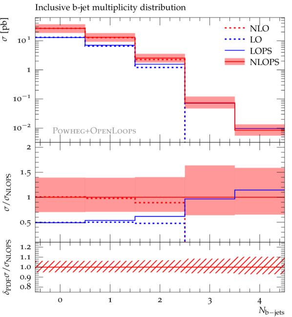
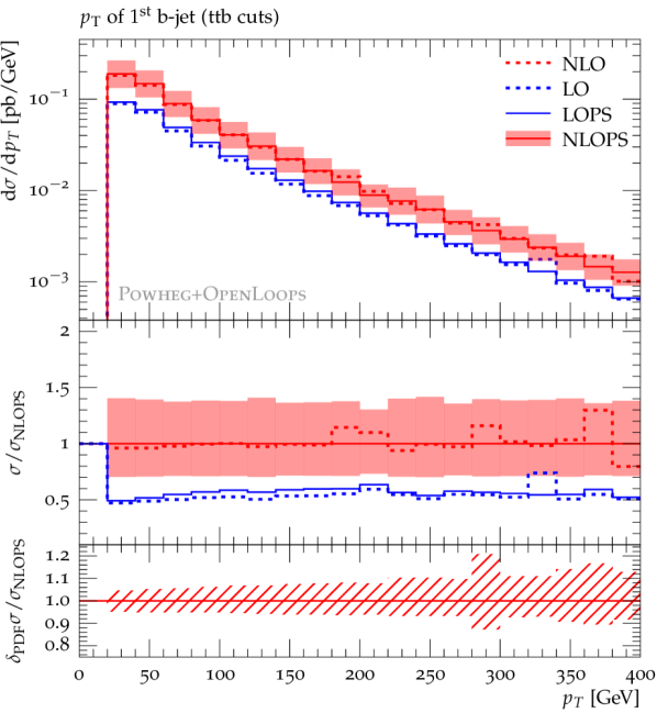
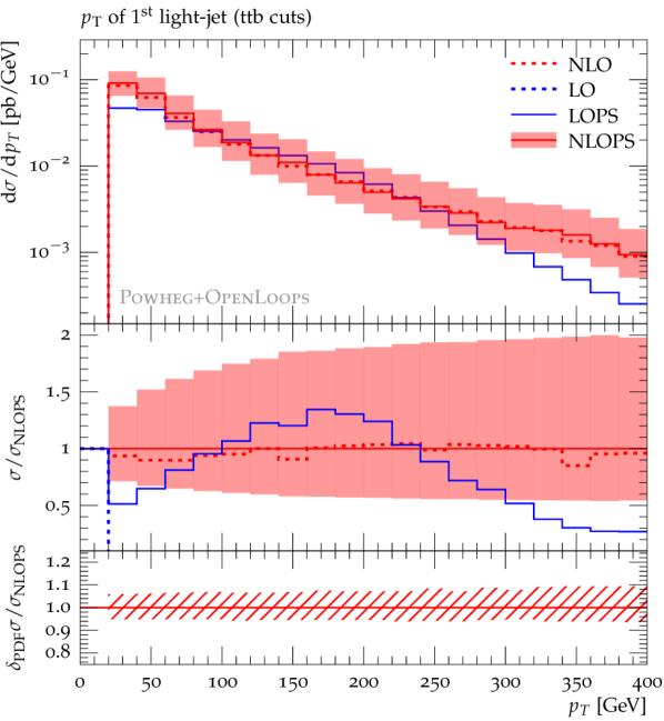
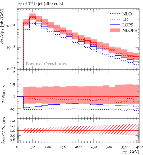
Figure 7: Predictions for $pp\to t\bar{t}b\bar{b}$ at $\sqrt{s}$=13 TeV: distributions in the inclusive number of additional $b$-jets (a), the $p_{\mathrm{T}}$ of the first $b$-jet (b) and the first light jet (c) with ttb cuts, and in the $p_{\mathrm{T}}$ of the second $b$-jet with ttbb cuts (d). Results at LO and NLO are in blue and red, respectively, and dashed lines correspond to fixed-order (N)LO predictions, while solid curves represent (N)LOPS predictions. The bands illustrate the envelope of 7-point $\mu_{\mathrm{R}},\mu_{\mathrm{F}}$ variations. Absolute predictions are shown in the main frame. The first ratio plot shows LO, LOPS and NLOPS predictions normalised to fixed-order NLO. The second ratio plot displays the relative effect of PDF uncertainties applied to NLOPS predictions Top quarks are kept stable throughout.

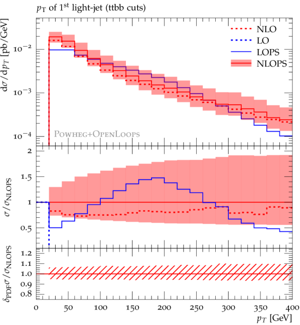
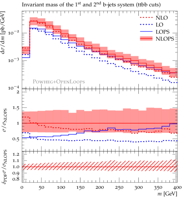
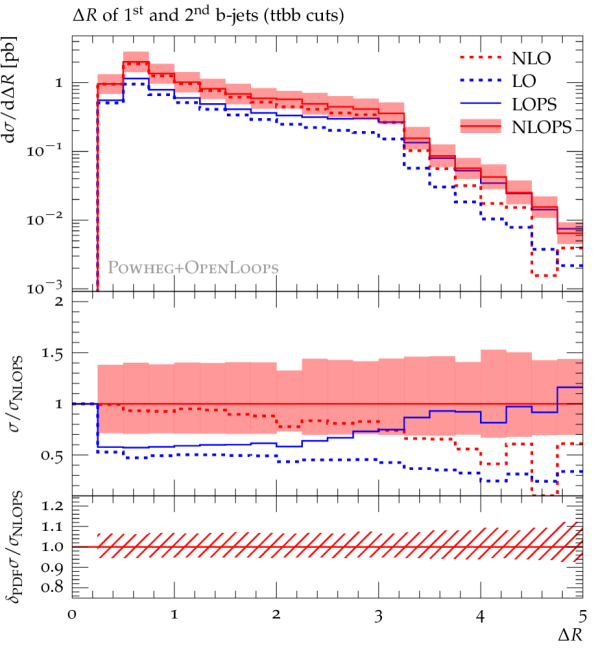
Figure 8: Distributions in the $p_{\mathrm{T}}$ of the second $b$-jet (a) in the $p_{\mathrm{T}}$ of the first light jet (b), and in the invariant mass (c) and the $\Delta R$ separation (d) of the first two $b$-jets with ttbb cuts throughout. Predictions and uncertainties as in Fig. 7.

Differential observables with ttb and ttbb cuts are presented in Figures 7–8. The inclusive $b$-jet multiplicity distribution in Fig. 7a extends the results of Table 1, which correspond to $N_{b}\geq 1,2$, to the bins with $N_{b}\geq 3,4$. The latter are populated by events that result from the interplay of real-emission matrix elements and $g\to b\bar{b}$ parton-shower splittings. Thus they feature an enhanced scale dependence.

For kinematic distributions that are inclusive with respect to NLO QCD radiation, NLOPS scale variations have a minor impact on shapes and amount essentially to a normalisation shift, similar to what observed at the level of the ttb and ttbb cross sections. In contrast, in the case of the light-jet $p_{\mathrm{T}}$ spectra, scale variations increase from about 30% in the soft region up to 100% in the hard tails. This is consistent with the fact that such observables are only LOPS accurate and depend on $\alpha_{\rm S}^{5}(\mu_{\rm R})$. The effect of PDF variations is clearly subleading as compared to scale uncertainties and has little impact on shapes.

Comparing (N)LOPS predictions to the respective fixed-order (N)LO results, we observe that matching and shower effects remain almost negligible also at the level of distributions in the ttb phase space. As for the ttbb region, the NLOPS effects of order 10% observed in $\sigma_{\mathrm{ttbb}}$ turn out to be quite sensitive to the kinematics of $b$-jets. In particular, as expected from the QCD dynamics of double $g\to b\bar{b}$ splittings Cascioli:2013era , the most pronounced effects are observed in the tails of the $m_{b_{1}b_{2}}$ and $\Delta R_{b_{1}b_{2}}$ distributions, where the NLOPS/NLO ratio approaches a factor two. In the Higgs signal region, $m_{b_{1}b_{2}}\sim 125$ GeV, the NLOPS enhancement is around 1.25 and well consistent with Ref. Cascioli:2013era .

Comparing fixed-order NLO predictions to LO ones we find that, in spite of the fairly large $K$-factors observed in Table 1, the shapes of distributions turn out to be quite stable with respect to higher-order QCD corrections. In the case of (N)LOPS predictions, the situation is different, especially for the shape of the light-jet $p_{\mathrm{T}}$ spectra, which receives significant NLO distortions. This is not surprising, since at LOPS the light-jet $p_{\mathrm{T}}$ is entirely generated by the parton shower. Thus the NLOPS/LOPS ratio should be regarded as a LO matrix-element correction to the parton-shower approximation, rather than a NLO correction in the perturbative sense.

Significant differences between NLOPS and LOPS shapes are observed also in the $m_{b_{1}b_{2}}$ and $\Delta R_{b_{1}b_{2}}$ distributions. Since the respective NLO and LO shapes are very similar, this behaviour can be attributed to the parton shower. More precisely, it can be understood as a side effect of the above-mentioned NLOPS/LOPS correction to the light-jet $p_{\mathrm{T}}$ spectra, which is converted into a double-splitting effect by $g\to b\bar{b}$ splittings inside the light jet.

4.2 Shower uncertainties

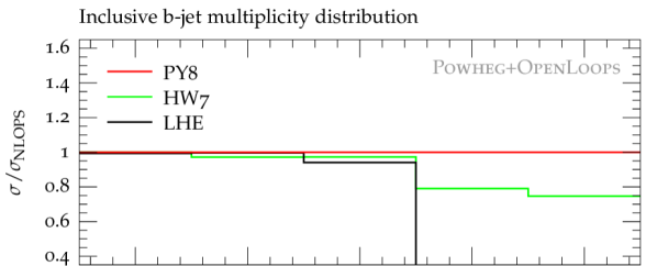
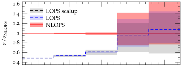
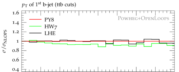
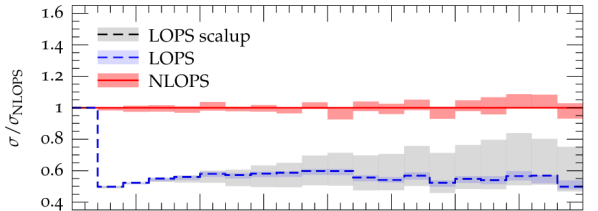
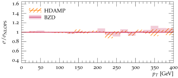
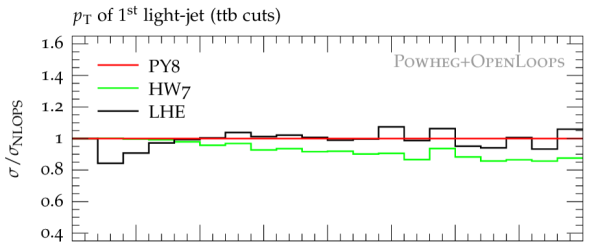
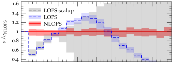
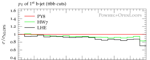
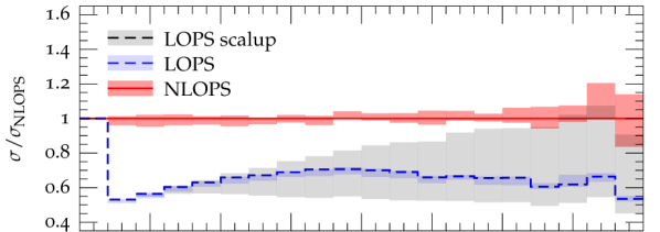
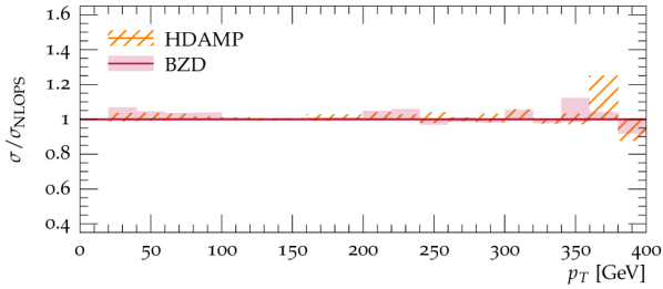
Figure 9: Relative impact of shower effects and uncertainties in (N)LOPS simulations of $pp\to t\bar{t}b\bar{b}$ at $\sqrt{s}$=13 TeV: distributions in the inclusive number of additional $b$-jets (a), the $p_{\mathrm{T}}$ of the first $b$-jet (b) and the first light jet (c) with ttb cuts, and in the $p_{\mathrm{T}}$ of the second $b$-jet with ttbb cuts (d). All results are normalised to nominal NLOPS predictions with Pythia 8. The upper frame compares NLOPS result based on Pythia 8 (PY8) or Herwig 7 (HW7) against LHE results. The central frame compares NLOPS (red) and LOPS (blue) predictions with uncertainties related to $\alpha_{\rm S}$ variations and to the modelling of $g\to b\bar{b}$ splittings in Pythia (red NLO band and blue LO band). At LOPS, also variations of the shower starting scale scalup=$H_{\mathrm{T}}/4,H_{\mathrm{T}}/2,H_{\mathrm{T}}$ are shown (grey band). The lower frame illustrates the relative effect of $h_{\mathrm{damp}}=H_{\mathrm{T}},H_{\mathrm{T}}/2,H_{\mathrm{T}},1.5m_{t}$ variations (HDAMP) and $h_{\mathrm{bzd}}=2,5,10$ variations (BZD). Top quarks are kept stable throughout.

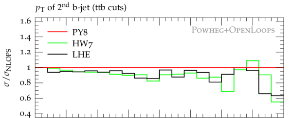
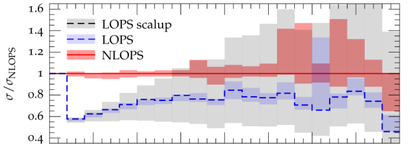
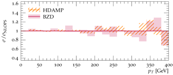
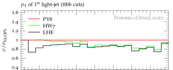
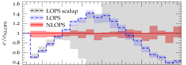
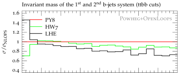
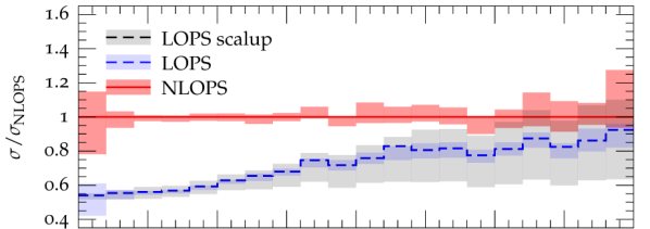
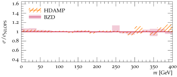
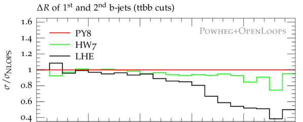
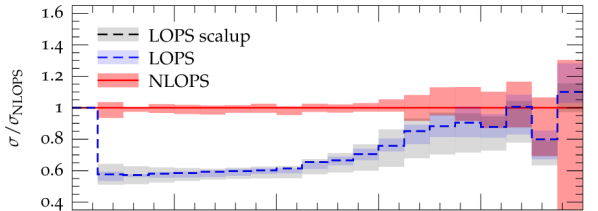
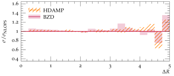
Figure 10: Distributions in the $p_{\mathrm{T}}$ of the second $b$-jet (a) in the $p_{\mathrm{T}}$ of the first light jet (b), and in the invariant mass (c) and the $\Delta R$ separation (d) of the first two $b$-jets with ttbb cuts throughout. Predictions and uncertainties as in Fig. 9.

In Figures 9–10 we study the sensitivity of (N)LOPS predictions to parton-shower and matching uncertainties for the same observables considered in Section 4.1.

The ratios displayed in the upper frames illustrate the net effect of parton showering by comparing full NLOPS predictions against results at LHE level. In addition, to assess parton-shower uncertainties, NLOPS predictions based on Pythia are compared to the corresponding results obtained with Herwig.

In the ttb phase space, apart from a mild distortion of the light-jet spectrum, the net effect of parton showering is essentially negligible. In contrast, in the ttbb phase space it increases the cross section by about 5% and tends to grow in the tails of distributions. The most sizable shower effects are observed in the $m_{b_{1}b_{2}}$ and $\Delta R_{b_{1}b_{2}}$ distributions, where they reach up to 50–100%. This behaviour is well consistent with the enhancement of the NLOPS/NLO ratio observed in Fig. 8, and the fact that it is driven by the parton shower provides further support to its interpretation in terms of double $g\to b\bar{b}$ splittings.

In spite of the important role of parton showering, it is reassuring to observe that the sensitivity of NLOPS predictions to the choice of parton shower is very small. In fact, the typical agreement between results based on Pythia and Herwig is at the level of a few percent both in the ttb and ttbb selections. Sizeable deviations at the level of 20% are observed only when requiring more than three $b$-jets. As discussed in Section 3.1, the very mild sensitivity of Powheg predictions to the choice of parton shower is due to the fact that the first emission is completely independent of the parton shower in the Powheg approach.

The ratios shown in the central frames of Figures 9–10 illustrate (N)LOPS uncertainties related to the modelling of $g\to b\bar{b}$ splittings and variations of $\alpha_{\rm S}$ in Pythia (see Section 3.3). At LOPS also variations of the shower starting scale (scalup) are shown.

The fact that $t\bar{t}b\bar{b}$ 4F matrix elements populate the whole $b\bar{b}$ phase space restricts the effect of $g\to b\bar{b}$ shower splittings to events with four or more $b$-quarks. Thus, only the cross sections with $N_{b}\geq 3,4$ $b$-jets suffer from sizable shower uncertainties. Vice versa, all considered observables with ttb or ttbb cuts turn out to be very stable, with typical shower uncertainties of a few percent at NLOPS. This holds also for the observables that are most sensitive to double splittings, i.e. $m_{b_{1}b_{2}}$ and $\Delta R_{b_{1}b_{2}}$, the only exception being the tail of the $\Delta R_{b\bar{b}}$ distribution, where double-splitting effects can reach 50% of the NLOPS cross section, while $g\to b\bar{b}$ shower uncertainties can reach 15%.

Predictions at LOPS depend also on the choice of the shower starting scale. This uncertainty is especially sizeable in the case of the light-jet spectrum, where scalup acts as a cutoff. A sizeable scalup dependence is visible also in the LOPS predictions for the $p_{\mathrm{T}}$-distributions of $b$-jets, which indicates that such observables are rather sensitive to QCD radiation. Let us recall that the scalup dependence disappears completely in NLOPS simulations based on the Powheg approach.

Ratios plotted in the lower frames of Figures 9–10 show the dependence of NLOPS predictions with respect to the choice of the $h_{\mathrm{damp}}$ and $h_{\mathrm{bzd}}$ parameters, which control the separation of the first emission into events of soft and hard type in the Powheg-Box framework (see Section 3.3). The $h_{\mathrm{damp}}$ band is obtained by varying $h_{\mathrm{damp}}=H_{\mathrm{T}}/4$, $H_{\mathrm{T}}/2$, $H_{\mathrm{T}}$, $1.5m_{t}$ with the value of $h_{\mathrm{bzd}}$ fixed to 2, while the $h_{\mathrm{bzd}}$ band is obtained by varying $h_{\mathrm{bzd}}=2$, $5$, $10$ with fixed $h_{\mathrm{damp}}=H_{\mathrm{T}}/2$. Observables that are inclusive with respect to light-jet radiation reveal a remarkably small dependence, typically of the order of a few percent, on the choice of $h_{\mathrm{damp}}$ and $h_{\mathrm{bzd}}$. Non-negligible but moderate uncertainties are found only in the light-jet spectra, which are enhanced by up to 20% when $h_{\mathrm{bzd}}$ is increased from 2 to 10. Investigating simultaneous variations of $h_{\mathrm{damp}}$ and $h_{\mathrm{bzd}}$ (not plotted) we have found that the size of the $h_{\mathrm{damp}}$ variation band is fairly stable with respect to the value of $h_{\mathrm{bzd}}$ within the considered range.

4.3 Comparisons against other $\boldsymbol{t\bar{t}b\bar{b}}$ and $\boldsymbol{t\bar{t}}$ generators

In Figures 11–12 we compare $t\bar{t}+b$-jet predictions based on Powheg+Pythia and Sherpa. This comparison is done both for (N)LOPS $pp\to t\bar{t}b\bar{b}$ generators in the 4F scheme and for corresponding generators of inclusive $t\bar{t}$ production in the 5F scheme. Specifically, in the case of Powheg we use hvq Frixione:2007nw . As detailed in Section 3.4, input parameters, QCD scales and matching parameters are chosen as coherently as possible across all generators. In this spirit, the parameter $h_{\mathrm{damp}}=H_{\mathrm{T}}/2$ in Powheg is identified with the resummation scale $\mu_{Q}$ in the SMC@NLO framework of Sherpa. Instead, for what concerns the parton showers we simply use standard settings, i.e. we do not try to improve the agreement between generators by tuning the Pythia and Sherpa showers.

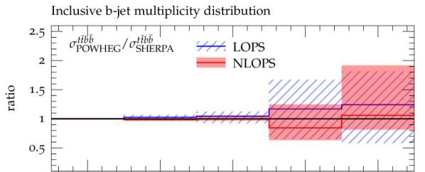
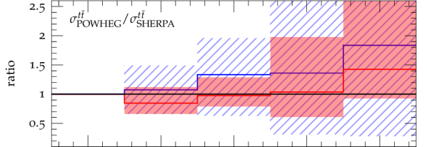
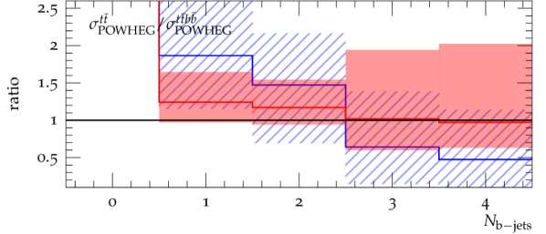
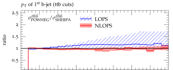
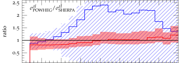
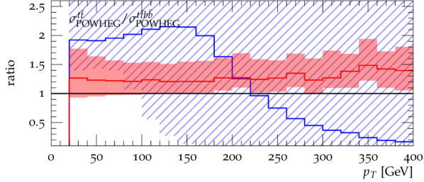
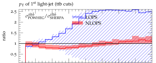
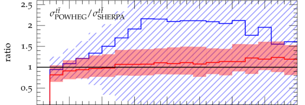
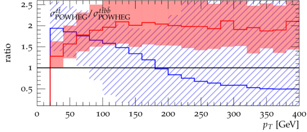
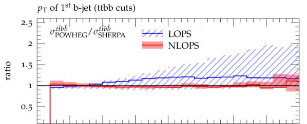
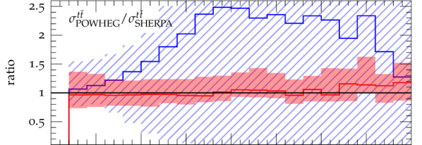
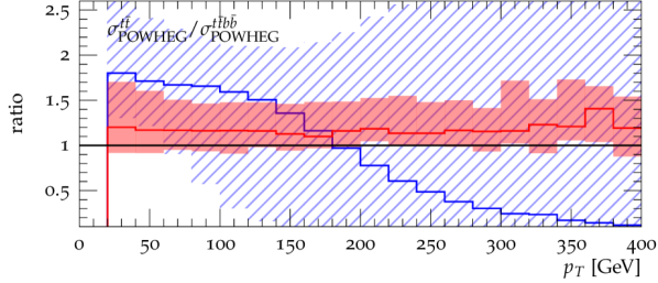
Figure 11: Predictions for $pp\to t\bar{t}+b$-jets at $\sqrt{s}$=13 TeV: distributions in the inclusive number of additional $b$-jets (a), the $p_{\mathrm{T}}$ of the first $b$-jet (b) and the first light jet (c) with ttb cuts, and in the $p_{\mathrm{T}}$ of the second $b$-jet with ttbb cuts (d). The various ratio plots compare $t\bar{t}+b$-jet observables as described in LOPS (blue) and NLOPS (red) simulations based on $pp\to t\bar{t}b\bar{b}$ or $pp\to t\bar{t}$ matrix elements in Powheg+Pythia or Sherpa. In the ratios shown in the upper and middle frame Powheg predictions are normalised to Sherpa ones for the case of $pp\to t\bar{t}b\bar{b}$ and $pp\to t\bar{t}$ simulations, respectively. The third frame displays the ratio of $t\bar{t}$ to $t\bar{t}b\bar{b}$ Powheg predictions. For all ratios the numerator and denominator are evaluated at the same order, and uncertainties are applied only to the numerator. They correspond to the combination in quadrature of $h_{\mathrm{damp}}$ and $h_{\mathrm{bzd}}$ variations with the uncertainties due to the modelling of $g\to b\bar{b}$ splittings and the choice of $\alpha_{\rm S}$ and scalup in Pythia (see Sections 3.2–3.3). Top quarks are kept stable throughout.

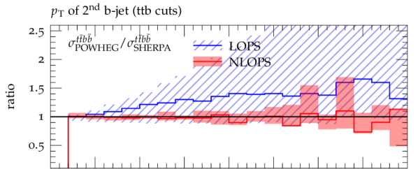
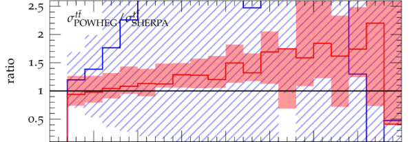
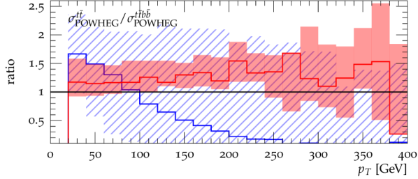
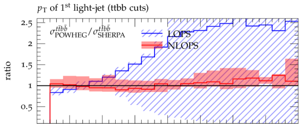
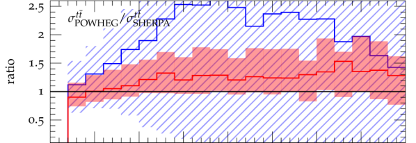
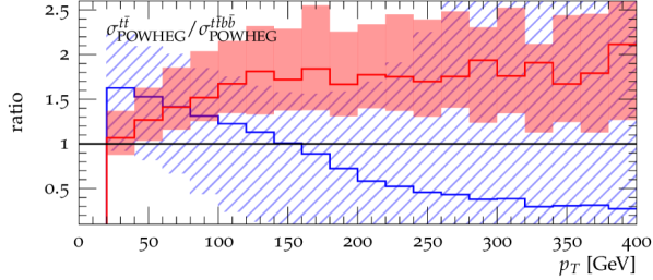
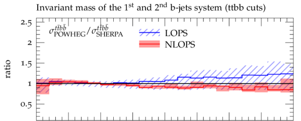
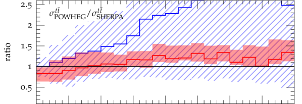
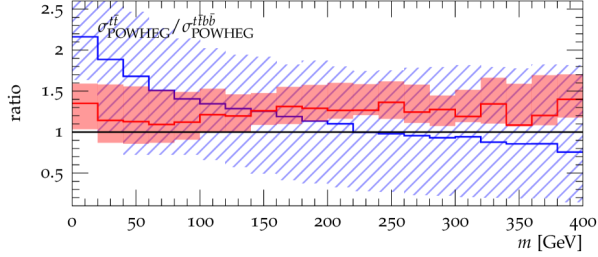
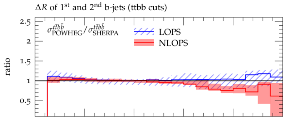
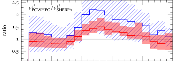
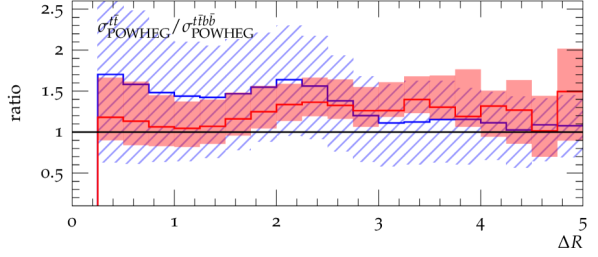
Figure 12: Distributions in the $p_{\mathrm{T}}$ of the second $b$-jet (a) in the $p_{\mathrm{T}}$ of the first light jet (b), and in the invariant mass (c) and the $\Delta R$ separation (d) of the first two $b$-jets with ttbb cuts throughout. Predictions and uncertainties as in Fig. 11.

The ratios in the upper frames of Figures 11–12 show Powheg $pp\to t\bar{t}b\bar{b}$ predictions normalised to corresponding Sherpa predictions at LOPS and NLOPS accuracy. The bands describe the combination in quadrature of all matching and shower uncertainties in Powheg+Pythia (referred to shower uncertainties in the following), while only nominal Sherpa predictions are considered in the ratios. Comparing LOPS predictions gives direct insights into the different modelling of radiation in Pythia and Sherpa. For observables that are inclusive with respect to jet radiation we find deviations between 10–40% and comparably large shower uncertainties. In contrast, in the jet-$p_{\mathrm{T}}$ distributions the LOPS predictions of Pythia are far above the ones by Sherpa, with differences that can reach a factor 2.5 in the tails. These differences are perfectly consistent with LOPS shower uncertainties, which are dominated by variations of the Pythia starting scale.

Moving to NLOPS reduces the direct dependence on the parton shower. At the same time, differences between the Powheg and SMC@NLO matching methods come into play. In practice, at NLOPS we observe a drastic reduction of shower uncertainties, especially in the light-jet and $b$-jet $p_{\mathrm{T}}$-distributions. Also the differences between Powheg and Sherpa become very small at NLOPS. The ttb and ttbb cross sections agree at the percent level, and differential $b$-jet observables deviate by more than 5% only in the tails of the $m_{b_{1}b_{2}}$ and $\Delta R_{b_{1}b_{2}}$ distributions. Even the light-jet spectra in the ttb and ttbb phase space deviate by less than 10–20% up to high $p_{\mathrm{T}}$, in spite of the limited formal accuracy (LOPS) of such observables. In the light of these results, NLOPS theoretical uncertainties related to the matching scheme and the parton shower seem to be well under control in $pp\to t\bar{t}b\bar{b}$. In particular, their impact appears to be clearly subleading as compared to QCD scale uncertainties.

In the central frames of Figures 11–12 we compare (N)LOPS generators of inclusive $t\bar{t}$ production based on Powheg+Pythia and Sherpa. In this case, the $g\to b\bar{b}$ final-state splittings that give rise to $t\bar{t}+b$-jet signatures are entirely controlled by the parton shower. At LOPS, also the parent gluon that splits into $b\bar{b}$ is generated by the parton shower. Nevertheless, the ttb and ttbb LOPS cross sections predicted by Powheg and Sherpa deviate by less than 30%–40%. Instead, as expected, the shapes of $t\bar{t}+b$-jet observables vary very strongly, and in all considered light-jet and $b$-jet distributions Pythia results exceed Sherpa ones by a factor of two and even more. This excess is well consistent with the estimated LOPS shower uncertainties. At NLOPS, only $g\to b\bar{b}$ splittings are controlled by the parton shower, while the emission of their parent gluon is dictated by LO matrix elements. Consequently, we observe a drastic reduction of shower uncertainties as compared to LOPS. Also the differences between Powheg and Sherpa are largely reduced at NLO, nevertheless they remain quite significant in various distributions.

To provide a more complete picture of the uncertainties of inclusive $t\bar{t}$ simulations, in the lower frames of Figures 11–12 we compare Powheg+Pythia generators of inclusive $t\bar{t}$ production and $t\bar{t}b\bar{b}$ production. Shower uncertainties are shown only for the $t\bar{t}$ generator. At LOPS, the $t\bar{t}$ generator is strongly sensitive to the modelling of $pp\to t\bar{t}g$ through initial-state gluon radiation in Pythia. As a result, the $t\bar{t}$ generator overestimates the ttb and ttbb cross sections by about 90% and 50%, respectively. This excess is strongly sensitive to scalup, and in the $p_{\mathrm{T}}$-distributions it is confined to the regions below 100–200 GeV, while the tails are strongly suppressed. Also the $m_{b_{1}b_{2}}$ and $\Delta R_{b_{1}b_{2}}$ distributions feature strong shape differences as compared to LOPS $t\bar{t}b\bar{b}$ predictions.

Such differences go down significantly at NLOPS. The ttb and ttbb cross sections predicted by the $t\bar{t}$ generator overshoot $t\bar{t}b\bar{b}$ results by only 15–20%, and also $b$-jet observables feature an improved agreement with $t\bar{t}b\bar{b}$ predictions. Nevertheless, in $b$-jet observables we find quite significant shape differences, especially for the $m_{b_{1}b_{2}}$ and $\Delta R_{b_{1}b_{2}}$ distributions, and shower uncertainties remain far above the ones of the $t\bar{t}b\bar{b}$ generator (see upper frame). As for the light-jet spectra, $t\bar{t}$ predictions turn out to lie above $t\bar{t}b\bar{b}$ ones by about a factor of two in the tails. In principle, with the help of parton shower tuning NLOPS $t\bar{t}$ generators may be amenable to a reasonable description of inclusive $t\bar{t}+b$-jet observables. However, in the light of the above results it should be clear that NLOPS $t\bar{t}b\bar{b}$ generators are mandatory in order to achieve an acceptable level of shower systematics.

5 $\boldsymbol{t\bar{t}b\bar{b}}$ production with top-quark decays

In this section we present NLOPS results of the Powheg+Pythia $t\bar{t}b\bar{b}$ generator with leptonic top-quark decays. More precisely we consider final states with oppositely charged leptons and/or muons. By default hadronisation and MPI are deactivated in Pythia, and their effect is shown separately. As detailed in Section 3.5, our implementation of top decays is based on resonant $pp\to t\bar{t}b\bar{b}\to 2\ell 2\nu b\bar{b}$(+j) matrix elements, where spin correlations are consistently taken into account.

Top-quark decays are due to weak interactions and, up to small corrections of $\mathcal{O}(\Gamma_{t}/m_{t})$, their effect factorises with respect to $t\bar{t}b\bar{b}$ production. Thus, while they strongly increase the complexity of $t\bar{t}+b$-jet events, top decays are not expected to interfere with the QCD dynamics of $pp\to t\bar{t}b\bar{b}$ in a significant way. In order to verify this hypothesis, in Fig. 13 we compare NLOPS $pp\to t\bar{t}b\bar{b}$ simulations with stable and decayed top quarks. To this end, based on Monte Carlo truth, all reconstructed jets are split into two subsets associated with $t\bar{t}b\bar{b}$ production and top decays. Specifically, jets that contain a parton originating from showered top-decay products are attributed to top decays, otherwise to $t\bar{t}b\bar{b}$ production. At the level of top decays we require two $b$-jets and two charged leptons within the acceptance cuts (39)–(40), while for the “reconstructed” $t\bar{t}b\bar{b}$ system we consider the same cuts and observables as for the case of stable top quarks. In order to mimic the leptonic branching ratio and the efficiency of acceptance cuts on top-decay products, the normalisation of the $t\bar{t}b\bar{b}$ simulation with stable top quarks is adapted to the predictions with decayed top quarks. This is done at the level of the ttbb cross section through a constant normalisation factor.

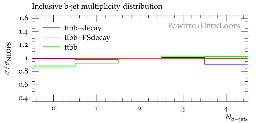
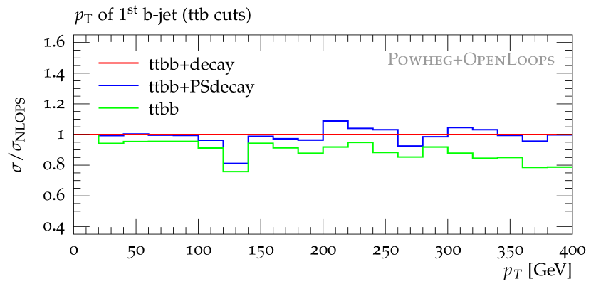
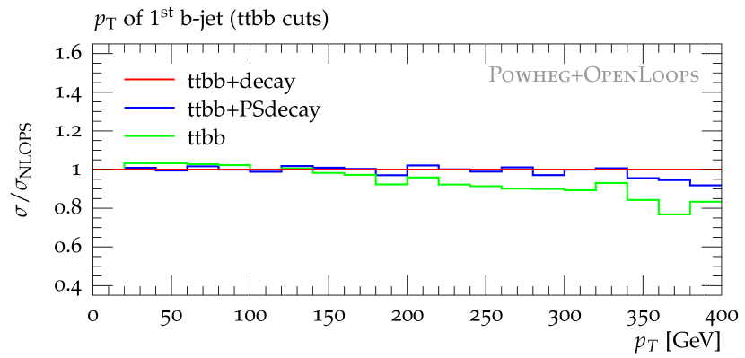
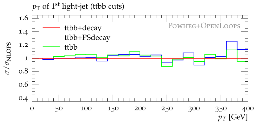
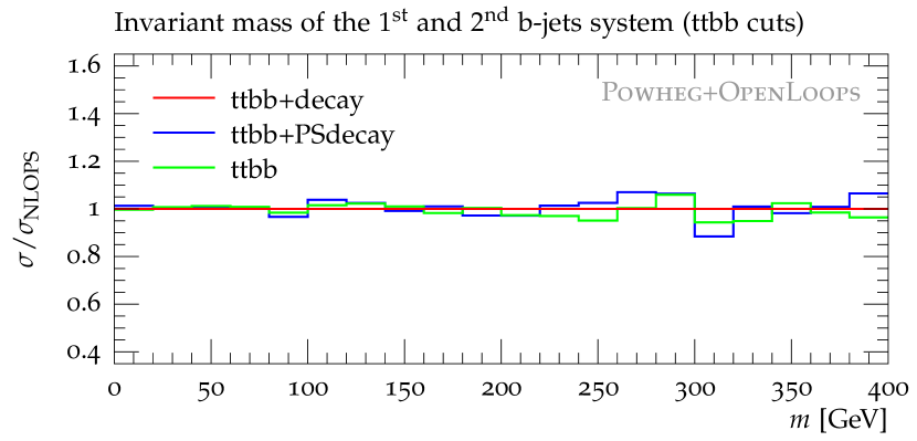
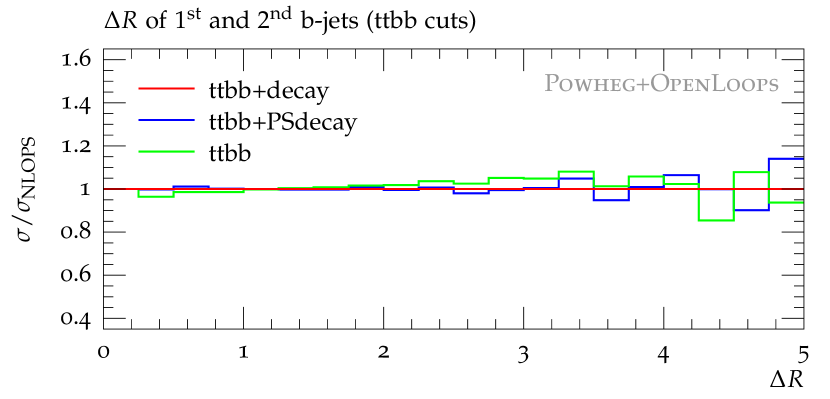
Figure 13: Distributions in the $b$-jets of the reconstructed $t\bar{t}b\bar{b}$ system for $pp\to t\bar{t}+b$-jets with dileptonic top decays at $\sqrt{s}$=13 TeV. Inclusive number of additional $b$-jets (a), distribution with ttb cuts in the $p_{\mathrm{T}}$ of the first $b$-jet (b) and distributions with ttbb cuts in the $p_{\mathrm{T}}$ of the first $b$-jet (c) and light-jet (d) as well as in the invariant mass (e) and $\Delta R$ (f) of the first and second $b$-jet. All results are based on Powheg+Pythia with hadronisation and MPI switched off. The ratio corresponds to NLOPS predictions with Pythia decays (ttbb+PSdecay) or stable top quarks (ttbb) normalised to corresponding ones with spin-correlated decays (ttbb+decay). Top-decay products are subject to acceptance cuts, while predictions with stable top quarks are normalised to ttbb+decay ones at the level of the ttbb cross section.

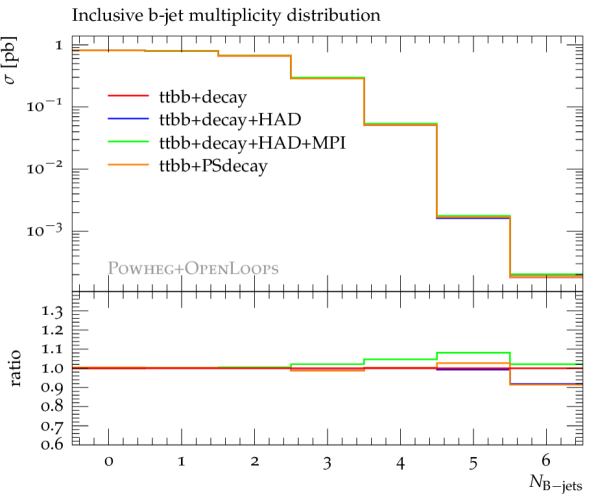
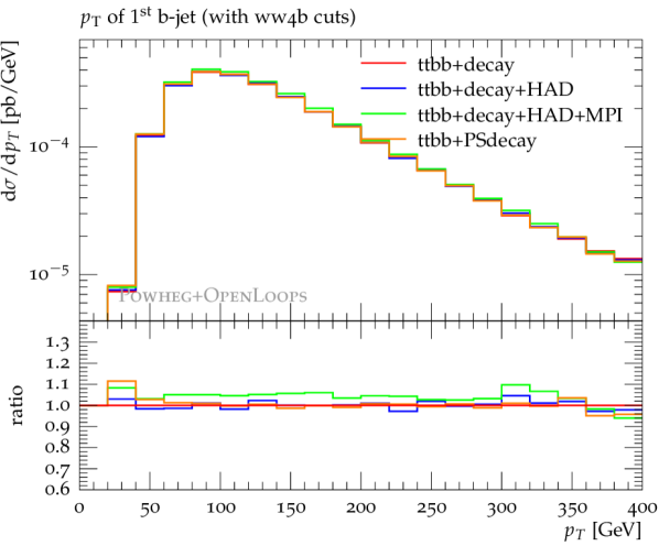
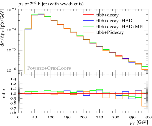
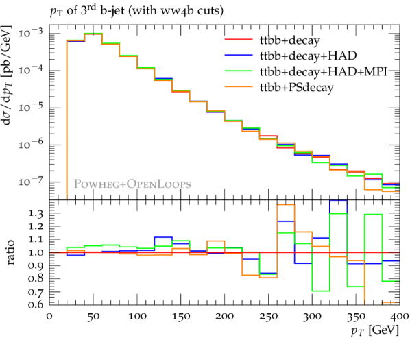
Figure 14: Predictions for $pp\to t\bar{t}+b$-jets at $\sqrt{s}$=13 TeV after leptonic top-quark decays. Four $b$-jets and two leptons within acceptance are required without any distinction between $b$-jets from $t\bar{t}b\bar{b}$ production and decay. Distributions in the inclusive number of $b$-jets (a) and in the $p_{\rm T}$ of the first (b), second (c) and third (d) $b$-jet. All results are based on Powheg+Pythia, and in the lower frame nominal NLOPS predictions with spin-correlated decays without (ttbb+decay) and with hadronisation (ttbb+decay+HAD) and multi-parton interactions (ttbb+decay+HAD+MPI) are compared to corresponding ones with Pythia decays (ttbb+PSdecay).

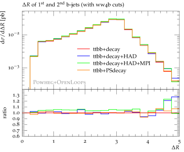
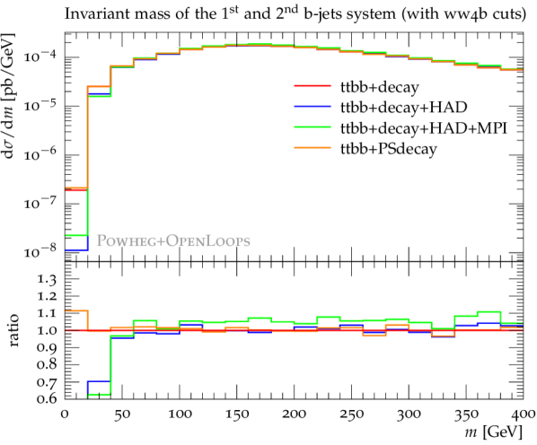
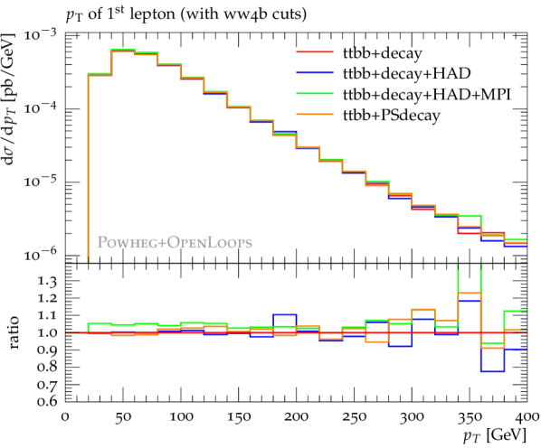
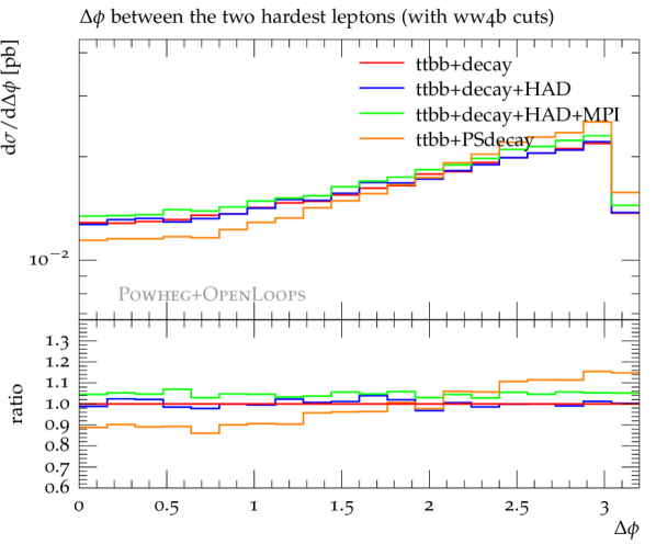
Figure 15: Distributions in the invariant mass (a) and $\Delta R$ (b) of the first and second $b$-jet, in the $p_{\rm T}$ of the leading lepton (c), and in the azimuthal $\Delta\phi$ separation of the two charged leptons (d). Predictions and ratios as in Fig. 14.

As shown in Fig. 13, $t\bar{t}+b$-jet observables with stable top quarks and reconstructed top decays turn out to agree quite well: $b$-jet cross sections and distributions deviate by only 5–10%, and also in the light-jet $p_{\mathrm{T}}$-distribution decay effects hardly exceed 10%. These differences can be understood as indirect effect of the acceptance cuts on top-decay products, which result from the correlation between the kinematics of the $t\bar{t}$ system and the additional jets.

Keeping in mind that realistic $b$-jet observables consist of a combinatorial superposition of $b$-jets from $t\bar{t}b\bar{b}$ production and from top decays, the fact that Monte Carlo truth acceptance cuts on top decays have only a minor effect on the production of $b$-jets suggests that the essential features observed in $pp\to t\bar{t}b\bar{b}$ production, such as double-splitting effects, are expected to show up also in the presence of top decays.

In order to assess the importance of spin correlations, in Fig. 13 we also compare spin-correlated top decays to isotropic decays generated by Pythia. At the level of reconstructed $t\bar{t}b\bar{b}$ observables this comparison does not reveal any significant effect of spin correlations.

A more realistic analysis of $t\bar{t}b\bar{b}$ production and decay is presented in Figures 14–15, where $b$-jet and leptonic observables are defined at the level of the full final state, and two charged leptons and four $b$-jets within the acceptance cuts (39)–(40) are required, without any distinction between $t\bar{t}b\bar{b}$ production and decay.

Comparing spin-correlated and isotropic top decays, in $b$-jet observables we find no significant deviation, and significant spin-correlation effects show up only in the azimuthal correlation of the two charged leptons.

In Figures 14–15 we also assess the relative impact of hadronisation and multi-parton interactions (MPI). It turns out that $b$-jet observables are very stable with respect to hadronisation, with differences between parton and hadron level that do not exceed the few percent level. The same holds for MPI effects.

The above results indicate that insights on the QCD dynamics of $t\bar{t}b\bar{b}$ production gained through studies with stable top quarks at parton level should hold true also in the presence of top decays and hadronisation.

6 Summary and conclusions

Searches for $t\bar{t}H$ production in the $H\to b\bar{b}$ channel call for a precise theoretical description of the irreducible $t\bar{t}+b$-jet background. To shed light on the QCD dynamics that governs this nontrivial multi-scale process, in the first part of this paper we have analysed the relative importance of the various mechanisms that lead to the radiation of $b$-quarks off $pp\to t\bar{t}$ events. To this end we have compared the role of $pp\to t\bar{t}b\bar{b}$ topologies involving initial-state and final-state $g\to b\bar{b}$ splittings. Using a naive diagrammatic splitting, as well as gauge-invariant collinear approximations, we have demonstrated that the $t\bar{t}+b$-jet cross section is strongly dominated by $b$-jet production via final-state $g\to b\bar{b}$ splittings. This holds both for phase space regions with two or only one resolved $b$-jets. These findings support the usage of NLOPS generators based on $pp\to t\bar{t}b\bar{b}$ matrix elements in the four-flavour scheme, while we have pointed out that $t\bar{t}+b$-jet predictions based on $t\bar{t}+$multi-jet merging rely very strongly on the parton-shower modelling of $g\to b\bar{b}$ splittings.

Motivated by these observations we have introduced a new $pp\to t\bar{t}b\bar{b}$ Powheg generator in the 4F scheme. This tool is based on the Powheg-Box-Res framework, and all relevant matrix elements are computed with OpenLoops. When applied to a multi-scale process like $pp\to t\bar{t}b\bar{b}$, the Powheg method can lead to subtle technical issues. In particular, we have pointed out that the FKS mappings which generate the recoil associated with the first Powheg emission can enhance the amplitude of the underlying $t\bar{t}b\bar{b}$ Born process in a way that leads to anomalously large weights as compared to the behaviour expected from the factorisation of soft and collinear radiation. Fortunately, such anomalies arise only from events with finite transverse momenta and not in the soft and collinear limits. Moreover, the Powheg-Box framework disposes of a mechanism that automatically attributes such events to the so-called finite remnant, where QCD radiation is handled as in fixed-order NLO calculations. This mechanism, which is controlled by the $h_{\mathrm{bzd}}$ parameter in (23), plays an important role for the efficiency of event generation. Moreover, it permits to avoid artefacts that can result from the application of QCD factorisation and resummation far away from their validity domain.

We have discussed predictions of the new Powheg generator and theoretical uncertainties for various $t\bar{t}+b$-jet cross sections and distributions at the 13 TeV LHC. At variance with previous studies, in order to provide a better picture of the perturbative convergence, we have evaluated QCD corrections using the same $\alpha_{\rm S}$ value and the same PDFs at LO and NLO. The resulting NLO $K$-factors turn out to be close to two, even if the renormalisation scale is chosen in a way that is expected to absorb large logarithms associated with the running of $\alpha_{\rm S}$. The question of the origin of such large higher-order effects and the search for possible remedies, such as improved scale choices, deserve to be addressed in future studies.

Scale uncertainties at fixed-order NLO amount to 25–30% and are dominated by renormalisation-scale variations. At NLOPS they tend to increase in a similar way as in Madgraph5aMC@NLO, while in Sherpa they tend to decrease deFlorian:2016spz . However this behaviour may be an artefact of the incomplete implementation of scale variations in NLOPS generators.

Comparing predictions at NLO, LHE and LOPS level reveals significant shower effects at the level of 10% in the ttbb cross section and up to 30% or more for the invariant-mass and $\Delta R$ distributions of $b$-jet pairs. These effects can be attributed to double $g\to b\bar{b}$ splittings Cascioli:2013era and are qualitatively and quantitatively consistent with the findings of Refs. Cascioli:2013era ; deFlorian:2016spz . For the $p_{\mathrm{T}}$-distribution of light-jet radiation, the predictions of the new Powheg generator are quite close to fixed-order NLO and also quite stable with respect to variations of the parameters $h_{\mathrm{damp}}$ and $h_{\mathrm{bzd}}$, which separate real radiation into singular and finite parts. This good stability is guaranteed by the $h_{\mathrm{bzd}}$-dependent mechanism mentioned above.

To assess pure shower uncertainties we have compared Powheg samples generated with Pythia 8 and Herwig 7. In addition, we have considered systematic uncertainties due to the modelling of $g\to b\bar{b}$ splittings and the choice of $\alpha_{\rm S}$ in Pythia. At NLOPS, all shower uncertainties turn out to be rather small and clearly subleading with respect to QCD scale variations. As a further independent estimate of matching and shower uncertainties we have compared NLOPS $t\bar{t}b\bar{b}$ generators based on Powheg+Pythia and Sherpa finding remarkable agreement both for $t\bar{t}+b$-jet cross sections and distributions. We have also shown that matching and shower uncertainties increase considerably if NLO corrections are not taken into account. The same holds for NLOPS generators of inclusive $t\bar{t}$ production as compared to $t\bar{t}b\bar{b}$ generators.

Finally, we have presented predictions for $pp\to t\bar{t}b\bar{b}$ with spin-correlated top decays. In this context we have show that hadronisation and MPI effects are almost negligible. Thus, the key features of the QCD dynamics of $t\bar{t}b\bar{b}$ production at parton level are expected to hold true also at particle level after top decays.

The new $t\bar{t}b\bar{b}$ Powheg generator will be made publicly available in the near future, and its application to experimental analyses may lead to significant steps forward in the understanding of the QCD dynamics of $t\bar{t}+b$-jet production and in the control of the theoretical uncertainties that plague $t\bar{t}H(b\bar{b})$ searches.

- (1) A. Bredenstein, A. Denner, S. Dittmaier, and S. Pozzorini, NLO QCD corrections to at the LHC, Phys. Rev. Lett. 103 (2009) 012002, [arXiv:0905.0110].
- (2) G. Bevilacqua, M. Czakon, C. G. Papadopoulos, R. Pittau, and M. Worek, Assault on the NLO Wishlist: , JHEP 09 (2009) 109, [arXiv:0907.4723].
- (3) A. Bredenstein, A. Denner, S. Dittmaier, and S. Pozzorini, NLO QCD Corrections to Top Anti-Top Bottom Anti-Bottom Production at the LHC: 2. full hadronic results, JHEP 03 (2010) 021, [arXiv:1001.4006].
- (4) M. V. Garzelli, A. Kardos, and Z. Trocsanyi, hadroproduction at NLO accuracy matched with parton shower, PoS EPS-HEP2013 (2013) 253.
- (5) M. V. Garzelli, A. Kardos, and Z. Trocsanyi, Hadroproduction of final states at LHC: predictions at NLO accuracy matched with Parton Shower, JHEP 03 (2015) 083, [arXiv:1408.0266].
- (6) P. Nason, A new method for combining NLO QCD with shower Monte Carlo algorithms, JHEP 11 (2004) 040, [hep-ph/0409146].
- (7) S. Frixione, P. Nason, and C. Oleari, Matching NLO QCD computations with Parton Shower simulations: the POWHEG method, JHEP 11 (2007) 070, [arXiv:0709.2092].
- (8) F. Cascioli, P. Maierhöfer, N. Moretti, S. Pozzorini, and F. Siegert, NLO matching for production with massive -quarks, Phys. Lett. B734 (2014) 210–214, [arXiv:1309.5912].
- (9) S. Höche, F. Krauss, M. Schönherr, and F. Siegert, A critical appraisal of NLO+PS matching methods, arXiv:1111.1220.
- (10) S. Frixione and B. R. Webber, Matching NLO QCD computations and parton shower simulations, JHEP 06 (2002) 029, [hep-ph/0204244].
- (11) LHC Higgs Cross Section Working Group Collaboration, D. de Florian et al., Handbook of LHC Higgs Cross Sections: 4. Deciphering the Nature of the Higgs Sector, arXiv:1610.07922.
- (12) J. Alwall, R. Frederix, S. Frixione, V. Hirschi, F. Maltoni, et al., The automated computation of tree-level and next-to-leading order differential cross sections, and their matching to parton shower simulations, JHEP 1407 (2014) 079, [arXiv:1405.0301].
- (13) G. Bevilacqua, M. V. Garzelli, and A. Kardos, hadroproduction with massive bottom quarks with PowHel, arXiv:1709.06915.
- (14) S. Catani, F. Krauss, R. Kuhn, and B. R. Webber, Qcd matrix elements + parton showers, JHEP 11 (2001) 063, [hep-ph/0109231].
- (15) M. L. Mangano, M. Moretti, and R. Pittau, Multijet matrix elements and shower evolution in hadronic collisions: + jets as a case study, Nucl. Phys. B632 (2002) 343–362, [hep-ph/0108069].
- (16) S. Hoeche, F. Krauss, S. Schumann, and F. Siegert, QCD matrix elements and truncated showers, JHEP 05 (2009) 053, [arXiv:0903.1219].
- (17) S. Höche, F. Krauss, M. Schönherr, and F. Siegert, QCD matrix elements + parton showers: The NLO case, arXiv:1207.5030.
- (18) L. Lonnblad and S. Prestel, Merging Multi-leg NLO Matrix Elements with Parton Showers, arXiv:1211.7278.
- (19) R. Frederix and S. Frixione, Merging meets matching in MC@NLO, JHEP 12 (2012) 061, [arXiv:1209.6215].
- (20) Talk by T. Ježo at 25th International Workshop on Deep Inelastic Scattering and Related Topics, https://indico.cern.ch/event/568360/contributions/2481300/.
- (21) Talk by T. Ježo at QCD@LHC 2017, https://indico.cern.ch/event/615220/contributions/2672600/.
- (22) T. Ježo and P. Nason, On the Treatment of Resonances in Next-to-Leading Order Calculations Matched to a Parton Shower, JHEP 12 (2015) 065, [arXiv:1509.09071].
- (23) http://powhegbox.mib.infn.it.
- (24) S. Frixione, P. Nason, and B. R. Webber, Matching NLO QCD and parton showers in heavy flavour production, JHEP 08 (2003) 007, [hep-ph/0305252].
- (25) S. Frixione, P. Nason, and G. Ridolfi, A Positive-Weight Next-to-Leading-Order Monte Carlo for Heavy Flavour Hadroproduction, JHEP 09 (2007) 126, [arXiv:0707.3088].
- (26) F. Maltoni, G. Ridolfi, and M. Ubiali, b-initiated processes at the LHC: a reappraisal, JHEP 1207 (2012) 022, [arXiv:1203.6393].
- (27) T. Gleisberg, S. Höche, F. Krauss, M. Schönherr, S. Schumann, F. Siegert, and J. Winter, Event generation with Sherpa 1.1, JHEP 02 (2009) 007, [arXiv:0811.4622].
- (28) S. Höche, F. Krauss, P. Maierhöfer, S. Pozzorini, M. Schönherr, and F. Siegert, Next-to-leading order QCD predictions for top-quark pair production with up to two jets merged with a parton shower, Phys. Lett. B748 (2015) 74–78, [arXiv:1402.6293].
- (29) F. Cascioli, P. Maierhöfer, and S. Pozzorini, Scattering Amplitudes with Open Loops, Phys.Rev.Lett. 108 (2012) 111601, [arXiv:1111.5206].
- (30) The OpenLoops one-loop generator by F. Cascioli, J. Lindert, P. Maierhöfer and S. Pozzorini is publicly available at http://openloops.hepforge.org.
- (31) F. Buccioni, S. Pozzorini, and M. Zoller, On-the-fly reduction of open loops, Eur. Phys. J. C78 (2018), no. 1 70, [arXiv:1710.11452].
- (32) T. Ježo, J. M. Lindert, P. Nason, C. Oleari, and S. Pozzorini, An NLO+PS generator for and production and decay including non-resonant and interference effects, Eur. Phys. J. C76 (2016), no. 12 691, [arXiv:1607.04538].
- (33) A. Denner, S. Dittmaier, and L. Hofer, COLLIER - A fortran-library for one-loop integrals, PoS LL2014 (2014) 071, [arXiv:1407.0087].
- (34) A. Denner and S. Dittmaier, Reduction of one loop tensor five point integrals, Nucl. Phys. B658 (2003) 175–202, [hep-ph/0212259].
- (35) A. Denner and S. Dittmaier, Reduction schemes for one-loop tensor integrals, Nucl. Phys. B734 (2006) 62–115, [hep-ph/0509141].
- (36) A. Denner and S. Dittmaier, Scalar one-loop 4-point integrals, Nucl. Phys. B844 (2011) 199–242, [arXiv:1005.2076].
- (37) G. Ossola, C. G. Papadopoulos, and R. Pittau, CutTools: a program implementing the OPP reduction method to compute one-loop amplitudes, JHEP 03 (2008) 042, [arXiv:0711.3596].
- (38) G. Ossola, C. G. Papadopoulos, and R. Pittau, Reducing full one-loop amplitudes to scalar integrals at the integrand level, Nucl. Phys. B763 (2007) 147–169, [hep-ph/0609007].
- (39) A. van Hameren, OneLOop: For the evaluation of one-loop scalar functions, Comput.Phys.Commun. 182 (2011) 2427–2438, [arXiv:1007.4716].
- (40) A. Buckley, J. Butterworth, L. Lönnblad, D. Grellscheid, H. Hoeth, J. Monk, H. Schulz, and F. Siegert, Rivet user manual, Comput. Phys. Commun. 184 (2013) 2803–2819, [arXiv:1003.0694].
- (41) S. Frixione, Z. Kunszt, and A. Signer, Three-jet cross sections to next-to-leading order, Nucl. Phys. B467 (1996) 399–442, [hep-ph/9512328].
- (42) S. Alioli, P. Nason, C. Oleari, and E. Re, A general framework for implementing NLO calculations in shower Monte Carlo programs: the POWHEG BOX, JHEP 06 (2010) 043, [arXiv:1002.2581].
- (43) S. Alioli, P. Nason, C. Oleari, and E. Re, NLO Higgs boson production via gluon fusion matched with shower in POWHEG, JHEP 0904 (2009) 002, [arXiv:0812.0578].
- (44) S. Alioli, P. Nason, C. Oleari, and E. Re, NLO vector-boson production matched with shower in POWHEG, JHEP 0807 (2008) 060, [arXiv:0805.4802].
- (45) NNPDF Collaboration, R. D. Ball et al., Parton distributions for the LHC Run II, JHEP 04 (2015) 040, [arXiv:1410.8849].
- (46) A. Buckley, J. Ferrando, S. Lloyd, K. Nordström, B. Page, M. Rüfenacht, M. Schönherr, and G. Watt, LHAPDF6: parton density access in the LHC precision era, Eur. Phys. J. C75 (2015) 132, [arXiv:1412.7420].
- (47) ATLAS Run 1 Pythia8 tunes, Tech. Rep. ATL-PHYS-PUB-2014-021, CERN, Geneva, Nov, 2014.
- (48) See http://home.thep.lu.se/~torbjorn/pythia82html/TimelikeShowers.html and http://home.thep.lu.se/Pythia/pdfdoc/g2qqbarsplit.pdf.
- (49) ATLAS Collaboration, G. Aad et al., Measurements of fiducial cross-sections for production with one or two additional b-jets in pp collisions at =8 TeV using the ATLAS detector, Eur. Phys. J. C76 (2016), no. 1 11, [arXiv:1508.06868].
- (50) J. Bellm et al., Herwig 7.0/Herwig++ 3.0 release note, Eur. Phys. J. C76 (2016), no. 4 196, [arXiv:1512.01178].
- (51) S. Höche, S. Schumann, and F. Siegert, Hard photon production and matrix-element parton-shower merging, Phys. Rev. D81 (2010) 034026, [arXiv:0912.3501].
- (52) S. Schumann and F. Krauss, A parton shower algorithm based on catani-seymour dipole factorisation, arXiv:0709.1027.
- (53) M. Czakon, P. Fiedler, and A. Mitov, Total Top-Quark Pair-Production Cross Section at Hadron Colliders Through , Phys. Rev. Lett. 110 (2013) 252004, [arXiv:1303.6254].
- (54) S. Frixione, E. Laenen, P. Motylinski, and B. R. Webber, Angular correlations of lepton pairs from vector boson and top quark decays in Monte Carlo simulations, JHEP 04 (2007) 081, [hep-ph/0702198].
- (55) S. Alioli, S.-O. Moch, and P. Uwer, Hadronic top-quark pair-production with one jet and parton showering, JHEP 01 (2012) 137, [arXiv:1110.5251].
- (56) H. B. Hartanto, B. Jager, L. Reina, and D. Wackeroth, Higgs boson production in association with top quarks in the POWHEG BOX, Phys. Rev. D91 (2015), no. 9 094003, [arXiv:1501.04498].
- (57) Particle Data Group Collaboration, C. Patrignani et al., Review of Particle Physics, Chin. Phys. C40 (2016), no. 10 100001.
- (58) M. Cacciari, G. P. Salam, and G. Soyez, The anti- jet clustering algorithm, JHEP 04 (2008) 063, [arXiv:0802.1189].
- (59) M. Cacciari, G. P. Salam, and G. Soyez, FastJet User Manual, Eur.Phys.J. C72 (2012) 1896, [arXiv:1111.6097].