Two-color Fermi liquid theory for transport through a multilevel Kondo impurity

Abstract

We consider a quantum dot with ${\cal K}{\geq}2$ orbital levels occupied by two electrons connected to two electric terminals. The generic model is given by a multi-level Anderson Hamiltonian. The weak-coupling theory at the particle-hole symmetric point is governed by a two-channel $S{=}1$ Kondo model characterized by intrinsic channels asymmetry. Based on a conformal field theory approach we derived an effective Hamiltonian at a strong-coupling fixed point. The Hamiltonian capturing the low-energy physics of a two-stage Kondo screening represents the quantum impurity by a two-color local Fermi-liquid. Using non-equilibrium (Keldysh) perturbation theory around the strong-coupling fixed point we analyse the transport properties of the model at finite temperature, Zeeman magnetic field and source-drain voltage applied across the quantum dot. We compute the Fermi-liquid transport constants and discuss different universality classes associated with emergent symmetries.

I Introduction

It is almost four decades since the seminal work of Nozieres and Blandin (NB) Nozieres and Blandin (1980) about the Kondo effect in real metals. The concept of the Kondo effect studied for impurity spin $S{=}1/2$ interacting with a single orbital channel ${\cal K}{=}1$ of conduction electrons Kondo (1964); Abrikosov (1965); Shul (1965); Anderson and Yuval (1969); Anderson et al. (1970); Abrikosov and Migdal (1970); Fowler and Zawadowski (1971); Noziéres (1974); Affleck (1990) was extended in Nozieres and Blandin (1980) for arbitrary spin $S$ and arbitrary number of channels ${\cal K}$. A detailed classification of possible ground states corresponding to the under-screened ${\cal K}{<}2S$, fully screened ${\cal K}{=}2S$ and overscreened ${\cal K}{>}2S$ Kondo effect has been given in Tsvelik and Wiegmann (1983); Andrei et al. (1983); Sacramento and Schlottmann (1991); Cox and Zawadowski (1998). Furthermore, it has been argued that in real metals the spin-$1/2$ single-channel Kondo effect is unlikely to be sufficient for the complete description of the physics of a magnetic impurity in a non-magnetic host. In many cases truncation of the impurity spectrum to one level is not possible and besides there are several orbitals of conduction-electrons which interact with the higher spin $S{>}1/2$ of the localized magnetic impurity Hewson (1993), giving rise to the phenomenon of multi-channel Kondo screening (Affleck and Ludwig, 1993; Coleman et al., 1995). In the fully screened case the conduction electrons completely screen the impurity spin to form a singlet ground state Andrei and Destri (1984). As a result, the low-energy physics is described by a local Fermi-Liquid (FL) theory Noziéres (1974); Nozieres and Blandin (1980). In the under-screened Kondo effect there exist not enough conducting channels to provide complete screening Posazhennikova and Coleman (2005); Koller et al. (2005). Thus, there is a finite concentration of impurities with a residual spin contributing to the thermodynamic and transport properties. In contrast to the underscreened and fully-screened cases, the physics of the overscreened Kondo effect is not described by the FL paradigm resulting in dramatic change of the thermodynamic and transport behaviour Hewson (1993).

$$\underbrace{\includegraphics[width=65.44142pt,valign={c}]{sc.pdf}}_{\rm second\;stage}\underbrace{\includegraphics[width=65.44142pt,valign={c}]{sb.pdf}}_{\rm first\;stage}\underbrace{\includegraphics[width=65.44142pt,valign={c}]{rs.pdf}}_{\rm weak\;coupling}$$

Figure 1: (Color online) Cartoon for non-monotonic behaviour of the differential conductance $G/G_{0}$ ($G_{0}=2e^{2}/h$ is the conductance quantum) as a function of temperature resulting from a two-stage Kondo effect. There are three characteristic regimes: (A) weak, (B) intermediate and (C) strong coupling. Crossover energy scales $T_{K}^{e}$ and $T_{K}^{o}$ are defined in the Section II. In the weak coupling (A)-regime the screening is absent (see top panel) and the transport coefficients are fully described by the perturbation theory Pustilnik and Glazman (2004). In the intermediate regime (B), the Kondo impurity is partially screened (see the first stage at the top panel); the residual interaction of electrons with the under-screened spin is antiferromagnetic Nozieres and Blandin (1980). The description of the FL transport coefficients in the strong coupling regime (C) at the second stage of the screening is the central result of the paper.

The simplest realization of the multi-channel fully screened Kondo effect is given by the model of a $S{=}1$ localized impurity screened by two conduction electron-channels. It has been predicted Pustilnik and Glazman (2004) that in spite of the FL universality class of the model, the transport properties of such FL are highly non-trivial. In particular, the screening develops in two stages (see Fig. 1), resulting in non-monotonic behaviour of the transport coefficients (see review Pustilnik and Glazman (2004) for details).

The interest in the Kondo effect revived during the last two decades due to progress in fabrication of nano-structures Kouwenhoven and Glazman (2001). Usually in nanosized objects such as quantum dots (QDs), carbon nanotubes (CNTs), quantum point contacts (QPCs) etc., Kondo physics can be engineered by fine-tuning the external parameters (e.g. electric and magnetic fields) and develops in the presence of several different channels of the conduction electrons coupled to the impurity. Thus, it was timely Pustilnik and Glazman (2001a, b); Kouwenhoven and Glazman (2001); Hofstetter and Schoeller (2002); Pustilnik et al. (2003); Hofstetter and Zarand (2004); Pustilnik and Glazman (2004) to uncover parallels between the Kondo physics in real metals and the Kondo effect in real quantum devices. The challenge of studying multi-channel Kondo physics Nozieres and Blandin (1980); Affleck and Ludwig (1993) was further revived in connection with possibilities to measure quantum transport in nano-structures experimentally Iftikhar et al. (2015); Keller et al. (2015); Potok et al. (2007); Ralph and Buhrman (1992, 1995); van der Wiel et al. (2002) inspiring also many new theoretical suggestions Matveev (1995a); Cox and Zawadowski (1998); Rosch et al. (2001); Oreg and Goldhaber-Gordon (2003); Posazhennikova and Coleman (2005); Posazhennikova et al. (2007); Kleeorin and Meir (2017).

Unlike the $S{=}1/2$, ${\cal K}{=}1$ Kondo effect (1CK), the two-channel $S{=}1$ Kondo problem suffers from lack of universality for its observables Nozieres and Blandin (1980). The reason is that certain symmetries (e.g. conformal symmetry) present in 1CK are generally absent in the two-channel $S{=}1$ model. This creates a major obstacle for constructing a complete theoretical description in the low-energy sector of the problem. Such a description should, in particular, account for a consistent treatment of the Kondo resonance (Affleck and Ludwig, 1993) appearing in both orbital channels. The interplay between two resonance phenomena, being the central reason for the non-monotonicity of transport coefficients Pustilnik and Glazman (2004), has remained a challenging problem for many years Posazhennikova and Coleman (2005); Posazhennikova et al. (2007).

A sketch of the temperature dependence of the differential electric conductance is shown on Fig. 1. The most intriguing result is that the differential conductance vanishes at both high and low temperatures, demonstrating the existence of two characteristic energy scales (see detailed discussion below). These two energy scales are responsible for a two-stage screening of $S{=}1$ impurity. Following Posazhennikova and Coleman (2005); Posazhennikova et al. (2007) we will refer to the $S{=}1$, ${\cal K}{=}2$ Kondo phenomenon as the two-stage Kondo effect (2SK).

While both the weak (A) and intermediate (B) coupling regimes are well-described by the perturbation theory Pustilnik and Glazman (2004), the most challenging and intriguing question is the study of strong-coupling regime (C) where both scattering channels are close to the resonance scattering. Indeed, the theoretical understanding of the regime C (in- and out-of-equilibrium) constitutes a long-standing problem that has remained open for more than a decade. Consequently, one would like to have a theory for the leading dependence of the electric current $I$ and differential conductance $G{=}\partial I/\partial V$ on magnetic field ($B$), temperature ($T$) and voltage ($V$),

$$G(B,T,V)/G_{0}=c_{B}B^{2}+c_{T}(\pi T)^{2}+c_{V}V^{2}.$$

Here $G_{0}{=}2e^{2}/h$ is unitary conductance. Computation of these parameters $c_{B}$, $c_{T}$ and $c_{V}$ using a local FL theory and to show how are these related constitute the main message of this work.

In this paper we offer a full-fledged theory of the two-stage Kondo model at small but finite temperature, magnetic field and bias voltage to explain the charge transport (current, conductance) behaviour in the strong-coupling regime of the 2SK effect. The paper is organized as follows. In Section II we discuss the multi-level Anderson impurity model along with different coupling regimes. The FL-theory of the 2SK effect in the strong-coupling regime is addressed in Section III. We outline the current calculations which account for both elastic and inelastic effects using the non-equilibrium Keldysh formalism in Section IV. In Section V we summarize our results for the FL coefficients in different regimes controlled by external parameters and discuss the universal limits of the theory. The Section VI is devoted to discussing perspectives and open questions. Mathematical details of our calculations are given in Appendices.

II Model

We consider a multi-level quantum dot sandwiched between two external leads $\alpha$ (${=}L,R$) as shown in Fig. 2. The generic Hamiltonian is defined by the Anderson model

$$H =\sum_{k\alpha\sigma}\left(\xi_{k}+\varepsilon_{\sigma}^{Z}\right)c^{\dagger}_{\alpha k\sigma}c_{\alpha k\sigma}+\sum_{\alpha ki\sigma}t_{\alpha i}c^{\dagger}_{\alpha k\sigma}d_{i\sigma}+\text{H.c.}$$

$$+\sum_{i\sigma}(\varepsilon_{i}+\varepsilon_{\sigma}^{Z})d^{\dagger}_{i\sigma}d_{i\sigma}+E_{c}\hat{\cal N}^{2}-{\cal J}\hat{\mathbf{S}}^{2},$$ (1)

where $c_{\alpha}$ stands for the Fermi-liquid quasiparticles of the source ($L$) and the drain ($R$) leads, $\xi_{k}=\varepsilon_{k}-\mu$ is the energy of conduction electrons with respect to the chemical potential $\mu$, and spin $\sigma=\uparrow{\color[rgb]{0,0,0}(+)},\downarrow{\color[rgb]{0,0,0}(-)}$ and $\varepsilon_{\sigma}^{Z}=-\sigma B/2$. The operator $d_{i\sigma}$ describes electrons with spin $\sigma$ in the $i$-th orbital state of the quantum dot and $t_{\alpha i}$ are the tunneling matrix elements, as shown in Fig. 2. Here $\varepsilon_{i}+\varepsilon_{\sigma}^{Z}$ is the energy of the electron in $i$-th orbital level of the dot in the presence of a Zeeman field $B$, $E_{c}$ is the charging energy (Hubbard interaction in the Coulomb blockade regime Matveev (1995b)), ${\cal J}\ll E_{c}$ is an exchange integral accounting for Hund’s rule Posazhennikova et al. (2007) and $\hat{\cal N}=\sum_{i\sigma}d^{\dagger}_{i\sigma}d_{i\sigma}$ is the total number of electrons in the dot. We assume that the dot is occupied by two electrons, and thus the expectation value of $\hat{\cal N}$ is $\bar{n}_{d}=2$ and the total spin $S=1$ (see Fig. 2). By applying a Schrieffer-Wolff (SW) transformation Schrieffer and Wolf (1966) to the Hamiltonian Eq. (II) we exclude single-electron states in the dot and project out the effective Hamiltonian, written in the $L$-$R$ basis, onto the spin-1 sector of the model:

$$H_{{\rm eff}}=\sum_{k\alpha\sigma}\xi_{k}c^{\dagger}_{\alpha k\sigma}c_{\alpha k\sigma}+\sum_{\alpha\alpha^{\prime}}J_{\alpha\alpha^{\prime}}\left[\textbf{s}_{\alpha\alpha^{\prime}}\cdot\textbf{S}\right],$$ (2)

with $\alpha,\alpha^{\prime}=L,R$, $B{=}0$ and

$$\mathbf{s}_{\alpha\alpha^{\prime}} =\frac{1}{2}\sum_{kk^{\prime}\sigma_{1}\sigma_{2}}c^{\dagger}_{\alpha k\sigma_{1}}\bm{\tau}_{\sigma_{12}}c_{\alpha^{\prime}k^{\prime}\sigma_{2}},$$ (3)

$$\mathbf{S} =\frac{1}{2}\sum_{{i\sigma_{1}\sigma_{2}}}d^{\dagger}_{i\sigma_{1}}\bm{\tau}_{\sigma_{12}}d_{i\sigma_{2}},$$ (4)

$$J_{\alpha\alpha^{\prime}} =\frac{2}{E_{c}}\left(\begin{array}[]{cc}|t_{L1}|^{2}+|t_{L2}|^{2}&t^{*}_{L2}t_{R2}+t^{*}_{L1}t_{R1}\\ t_{L2}t^{*}_{R2}+t_{L1}t^{*}_{R1}&|t_{R2}|^{2}+|t_{R1}|^{2}\\ \end{array}\right),$$ (7)

where we use the short-hand notation $\bm{\tau}_{\sigma_{ij}}\equiv\bm{\tau}_{\sigma_{i}\sigma_{j}}$ for the Pauli matrices.

The determinant of the matrix $J_{\alpha\alpha^{\prime}}$ in Eq. (7) is non-zero provided that $t_{L2}t_{R1}{\neq}t_{L1}t_{R2}$. Therefore, one may assume without loss of generality that both eigenvalues of the matrix $J_{\alpha\alpha^{\prime}}$ are non-zero and, hence, both scattering channels interact with the dot. There are, however, two important cases deserving an additional discussion. The first limiting case is achieved when two eigenvalues of $J_{\alpha\alpha^{\prime}}$ are equal and the matrix $J_{\alpha\alpha^{\prime}}$ is proportional to the unit matrix in any basis of electron states of the leads. As a result, the net current through impurity vanishes at any temperature, voltage and magnetic field Posazhennikova et al. (2007) (see Fig. 1, showing that the differential conductance vanishes when symmetry between channels emerges). This is due to destructive interference between two paths Posazhennikova et al. (2007) (Fig. 2) occurring when e.g. $t_{L1}{=}t_{L2}{=}t_{R1}{=}t$, $t_{R2}{=}-t$. Precise calculations done later in the paper highlight the role of destructive interference effects and quantify how the current goes to zero in the vicinity of the symmetry point. The second limiting case is associated with constructive interference between two paths (Fig. 2) when $t_{L1}{=}t_{L2}{=}t_{R1}{=}t_{R2}{=}t$. In that case the determinant of the matrix $J_{\alpha\alpha^{\prime}}$ in Eq. (7) and thus also one of the eigenvalues of $J_{\alpha\alpha^{\prime}}$, is zero. As a result, the corresponding channel is completely decoupled from the impurity. The model then describes the under-screened $S{=}1$ single-channel Kondo effect.

Applying the Glazman-Raikh rotation Glazman and Raikh (1988) $b^{\dagger}_{e/o}{=}(c^{\dagger}_{L}{\pm}c^{\dagger}_{R})/\sqrt{2}$ to the effective Hamiltonian Eq. (2) we re-write the Kondo Hamiltonian in the diagonal basis symcop , introducing two coupling constants $J_{e}$, $J_{o}$

$$\mathcal{H}_{\rm eff} =\sum_{a}\left(H^{a}_{0}+J_{a}\mathbf{s}_{a}\cdot\mathbf{S}\right).$$ (8)

In writing Eq. (8) we assigned the generalized index $``a"$ to represent the even and odd channels $(a{=}e,o)$. $H^{a}_{0}{=}\sum_{ak\sigma}(\varepsilon_{k}{-}\mu)b^{\dagger}_{ak\sigma}b^{\phantom{\dagger}}_{ak\sigma}$ is the non-interacting Hamiltonian of channel $a$ in the rotated basis. The spin density operators in the new basis are: $\mathbf{s}_{a}{=}1/2\sum_{kk^{\prime}\sigma_{1}\sigma_{2}}b^{\dagger}_{ak\sigma_{1}}\bm{\tau}_{\sigma_{12}}b_{ak^{\prime}\sigma_{2}}$. For equal leads-dot coupling, the $J_{a}$ are of the order of $t^{2}/E_{c}$. The interaction between even and odd channels is generated by the next non-vanishing order of Schrieffer-Wolff transformation

$$H_{eo}=-J_{eo}\mathbf{s}_{e}\cdot\mathbf{s}_{o}$$ (9)

where $J_{eo}$ is estimated as $J_{eo}{\sim}J_{e}J_{o}/{\color[rgb]{0,0,0}\max[E_{c},\mu]}$. As a result this term is irrelevant in the weak coupling regime. However, we note that the sign of $J_{eo}$ is positive, indicating the ferromagnetic coupling between channels necessary for the complete screening of the $S=1$ impurity Nozieres and Blandin (1980) (see Fig. 1).

$$\underbrace{\includegraphics[width=110.96556pt,valign={c}]{h_2.pdf}}_{\rm S=1}\underbrace{\includegraphics[width=110.96556pt,valign={c}]{h_1.pdf}}_{\rm S=1}$$

Figure 2: (Color online) Cartoon of some possible realization of a multi-orbital Anderson model setup: two degenerate $p$-orbitals (magenta and green) of a quantum dot are occupied by one electron each forming a triplet $S{=}1$ state in accordance with the Hund’s rule (see lower panel). The third $p$-orbital (not shown) is either empty or doubly occupied. Two limiting cases are important: i) totally constructive interference $t_{L1}{=}t_{L2}{=}t_{R1}{=}t_{R2}{=}t$; ii) totally destructive interference $t_{L1}{=}t_{L2}{=}t_{R1}{=}t$, $t_{R2}{=}-t$. Besides, if $t_{L2}{=}t_{R2}{=}0$, only one orbital is coupled to the leads, resulting in the 1CK model. If $t_{L2}{=}t_{R1}{=}0$, each orbital is coupled to a “dedicated lead” and the net current through the dot is zero.

The Hamiltonian (8) describes the weak coupling limit of the two-stage Kondo model. The coupling constants $J_{e}$ and $J_{o}$ flow to the strong coupling fixed point (see details of the renormalization group (RG) analysis Anderson (1970); Abrikosov and Migdal (1970); Fowler and Zawadowski (1971) in Appendix A.1). In the leading-$\log$ (one loop RG) approximation, the two channels do not talk to each other. As a result, two effective energy scales emerge, referred as Kondo temperatures, $T_{K}^{a}=D\exp(-1/(2N_{F}J_{a}))$ ($D$ is a bandwidth and $N_{F}$ is 3-dimensional electron’s density of states in the leads). These act as crossover energies, separating three regimes: the weak-coupling regime, $T\gg\max[T_{K}^{a}]$ (see Appendix  A.1); the intermediate regime, $\min[T_{K}^{a}]\ll T\ll\max[T_{K}^{a}]$ characterized by an incomplete screening (see Fig. 1) when one conduction channels (even) falls into a strong coupling regime while the other channel (odd) still remains at the weak coupling (see Appendix  A.2); and the strong-coupling regime, $T\ll\min[T_{K}^{a}]$. In the following section we discuss the description of the strong coupling regime by a local Fermi-liquid paradigm.

III Fermi-Liquid Hamiltonian

The RG analysis of the Hamiltonian (8) (see Appendix A.1 for details) shows that the 2SK model has a unique strong coupling fixed point corresponding to complete screening of the impurity spin. This strong-coupling fixed point is of the FL-universality class. In order to account for existence of two different Kondo couplings in the odd and even channels and the inter-channel interaction, we conjecture that the strong-coupling fixed point Hamiltonian contains three leading irrelevant operators:

$$H=-\sum_{aa^{\prime}}\lambda_{aa^{\prime}}:\!\mathbf{s}_{a}(0)\cdot\mathbf{s}_{a^{\prime}}(0)\!:\;,$$ (10)

with $\lambda_{ee}{=}\lambda_{e}$, $\lambda_{oo}{=}\lambda_{o}$ and $\lambda_{eo}{=}\lambda_{oe}$. The notation $:...:$ corresponds to a normal ordering where all divergences originating from bringing two spin currents $\mathbf{s}_{a}$ close to each other are subtracted. The conjecture (10) is in the spirit of Affleck’s ideas Affleck and Ludwig (1993) of defining leading irrelevant operators of minimal operator dimension being simultaneously (i) local, (ii) independent of the impurity spin operator $\mathbf{S}$, (iii) rotationally invariant and (iv) independent of the local charge density. We do not assume any additional (SO(3) or SU(2)) symmetry in the channel subspace except at the symmetry-protected point $\lambda_{e}{=}\lambda_{o}{=}\lambda_{eo}{=}\lambda$. At this symmetry point a new conservation law for the total spin current (Affleck and Ludwig, 1993) emerges and the Hamiltonian reads as

$$H=-\lambda:\!\mathbf{S}(0)\cdot\mathbf{S}(0)\!:,\;\;\;\;\;\mathbf{S}=\mathbf{s}_{e}+\mathbf{s}_{o}.$$

This symmetric point is obtained with the condition $J_{e}{=}J_{o}$ in $H_{{\rm eff}}$, see Eq. (8). Under this condition, as has been discussed in the previous section, the net current through the impurity is zero due to totally destructive interference. This symmetry protects the zero-current state at any temperature, magnetic and/or electric field (see Fig. 2).

Applying the point-splitting procedure Affleck and Ludwig (1993); Hanl et al. (2014) to the Hamiltonian Eq. (10), we get $H=H_{e}+H_{o}+H_{eo}$ with

$$H_{a} ={-}\tfrac{3}{4}i\lambda_{a}\sum_{\sigma}\left[b^{\dagger}_{a\sigma}\tfrac{d}{dx}b^{\phantom{\dagger}}_{a\sigma}{-}\left(\tfrac{d}{dx}b^{\dagger}_{a\sigma}\right)b^{\phantom{\dagger}}_{a\sigma}\right]{+}\tfrac{3}{2}\lambda_{a}\rho_{a\uparrow}\rho_{a\downarrow},$$

$$H_{eo} =-\lambda_{eo}\left[:\!\mathbf{s}_{e}(0)\cdot\mathbf{s}_{o}(0)+\mathbf{s}_{o}(0)\cdot\mathbf{s}_{e}(0)\!:\right].$$ (11)

The Hamiltonian Eq. (III) accounts for two copies of the $s{=}1/2$ Kondo model at strong coupling with an additional ferromagnetic interaction between the channels providing complete screening at $T{=}0$.

An alternative derivation of the strong-coupling Hamiltonian (III) can be obtained, following Refs. Mora (2009); Mora et al. (2015); Filippone et al. (2017), with the most general form of the low-energy FL Hamiltonian. For the two-stage Kondo problem corresponding to the particle-hole symmetric limit of the two-orbital-level Anderson model, it is given by $H=H_{0}+H_{\alpha}+H_{\phi}+H_{\Phi}$ with

$$H_{0} {=}\phantom{-}\sum_{a\sigma}\int_{\varepsilon}\nu\left(\varepsilon+\varepsilon_{\sigma}^{Z}\right)b^{\dagger}_{a\varepsilon\sigma}b^{\phantom{\dagger}}_{a\varepsilon\sigma}$$

$$H_{\alpha} {=}{-}\sum_{a\sigma}\int_{\varepsilon_{1-2}}\frac{\alpha_{a}}{2\pi}\left(\varepsilon_{1}+\varepsilon_{2}\right)\!b^{\dagger}_{a\varepsilon_{1}\sigma}b^{\phantom{\dagger}}_{a\varepsilon_{2}\sigma}\!$$

$$H_{\phi} {=}\phantom{-}\sum_{a}\int_{\varepsilon_{1-4}}\frac{\phi_{a}}{\pi\nu}:\!b^{\dagger}_{a\varepsilon_{1}\uparrow}b_{a\varepsilon_{2}\uparrow}b^{\dagger}_{a\varepsilon_{3}\downarrow}b_{a\varepsilon_{4}\downarrow}\!:$$

$$H_{\Phi} {{=}}{{-}}{\sum_{\sigma_{{1{-}4}}}}{\int_{\varepsilon_{{1{{-}}4}}}}{{\frac{\Phi}{{2}{\pi}{\nu}}}}{{:}b^{{\dagger}}_{{o\varepsilon_{1}\sigma_{1}}}{\bm{\tau}_{{{\sigma_{12}}}}}{b_{{o\varepsilon_{2}\sigma_{2}}}}{b^{{\dagger}}_{e\varepsilon_{3}\sigma_{3}}{\bm{\tau}_{\sigma_{34}}}b_{e\varepsilon_{4}\sigma_{4}}{:}}}{,}$$ (12)

where $\nu{=}1/(2\pi\hbar v_{F})$ is the density of states per species for a one-dimensional channel. In Eq. (12) $H_{\alpha}$ describes energy-dependent elastic scattering Affleck and Ludwig (1993). The inter and intra-channel quasiparticle interactions responsible for the inelastic effects are described by $H_{\Phi}$ and $H_{\phi}$ respectively. The particle-hole symmetry of the problem forbids to have any second-generation of FL-parameters Mora (2009) in Eq. (12). Therefore, the Hamiltonian Eq. (12) constitutes a minimal model for the description of a local Fermi-liquid with two interacting resonance channels. The direct comparison of the above FL-Hamiltonian with the strong-coupling Hamiltonian Eq. (III) provides the relation between the FL-coefficients at PH symmetry, namely $\alpha_{a}{=}\phi_{a}$ The Kondo floating argument (see Mora (2009)) recovers this relation. As a result we have three independent FL-coefficients $\alpha_{e}$, $\alpha_{o}$ and $\Phi$ which can be obtained from three independent measurements of the response functions. The FL-coefficients in Eq. (12) are related to the leading irrelevant coupling parameters $\lambda$’s in Eq. (III) as

$$\alpha_{a} =\phi_{a}=\frac{3\lambda_{a}\pi}{2}\;\;\text{and}\;\;\Phi=\pi\lambda_{eo},$$ (13)

The symmetry point $\lambda_{e}{=}\lambda_{o}{=}\lambda_{eo}{=}\lambda$ constrains $\alpha_{e}{=}\alpha_{o}{=}3\Phi/2$ in the Hamiltonian Eq. (12).

To fix three independent FL parameters in (12) in terms of physical observables, three equations are needed. Two equations are provided by specifying the spin susceptibilities of two orthogonal channels. The remaining necessary equation can be obtained by considering the impurity contribution to specific heat. It is proportional to an impurity-induced change in the total density of states per spin Hewson (1993), $\nu^{\rm imp}_{a\sigma}(\varepsilon){=}\frac{1}{\pi}\partial_{\varepsilon}\delta^{a}_{\sigma}(\varepsilon)$, where $\delta^{a}_{\sigma}(\varepsilon)$ are energy dependent scattering phases in odd and even channels (see the next Section for more details)

$$\frac{C^{\rm imp}}{C_{\rm bulk}}=\frac{\sum_{a\sigma}\frac{1}{\pi}\partial_{\varepsilon}\delta_{\sigma}^{a}(\varepsilon)|_{\varepsilon=0}}{4\nu}=\frac{\alpha_{e}+\alpha_{o}}{2\pi\nu}\;.$$ (14)

The quantum impurity contributions to the spin susceptibilities of the odd and even channels (see details in Hanl et al. (2014)) are given by

$$\frac{\chi^{\text{imp}}_{e}}{\chi_{\text{bulk}}}=\frac{\alpha_{e}+\Phi/2}{\pi\nu},\;\;\;\;\;\;\;\;\;\;\;\;\frac{\chi^{\text{imp}}_{o}}{\chi_{\text{bulk}}}=\frac{\alpha_{o}+\Phi/2}{\pi\nu}.$$ (15)

The equations (14-15) fully determine three FL parameters $\alpha_{e}$, $\alpha_{o}$ and $\Phi$ in (12). Total spin susceptibility $\chi^{\text{imp}}{=}\chi^{\text{imp}}_{e}{+}\chi^{\text{imp}}_{o}$ together with the impurity specific heat (14) defines the Wilson ratio, $R{=}(\chi^{\text{imp}}/\chi_{\text{bulk}})/(C^{\text{imp}}/C_{\text{bulk}})$ Affleck and Ludwig (1993), Gogolin et al. (1998) which measures the ratio of the total specific heat to the contribution originating from the spin degrees of freedom

$$R=2\left[\frac{\alpha_{e}+\alpha_{o}+\Phi}{\alpha_{e}+\alpha_{o}}\right]=2\left[1+\frac{2}{3}\frac{\lambda_{eo}}{\lambda_{e}+\lambda_{o}}\right].$$ (16)

For $\lambda_{e}{=}\lambda_{o}{=}\lambda_{eo}$, Eq. (16) reproduces the value $R{=}8/3$ known for the two-channel, fully screened $S{=}1$ Kondo model Affleck (1995). If however $\lambda_{eo}{=}0$ we get $R{=}2$, in agreement with the text-book result for two not necessarily identical but independent replicas of the single channel Kondo model.

IV Charge Current

The current operator at position $x$ is expressed in terms of first-quantized operators $\psi$ attributed to the linear combinations of the Fermi operators in the leads

$$\hat{I}(x){=}\frac{e\hbar}{2mi}\sum_{\sigma}\left[\psi^{\dagger}_{\sigma}(x)\partial_{x}\psi_{\sigma}(x)-\partial_{x}\psi^{\dagger}_{\sigma}(x)\psi_{\sigma}(x)\right].$$ (17)

In the present case both types of quasi-particles $b_{ak\sigma}(a{=}e,o)$ interact with the dot. Besides, both scattering phases ($e/o$) are close to their resonance value $\delta^{e/o}_{0,\sigma}{=}\pi/2$. This is in striking contrast to the single channel Kondo model, where one of the eigenvalues of the $2\times 2$ matrix of $J_{\alpha\alpha^{\prime}}$ in Eq. (7) is zero, and hence the corresponding degree of freedom is completely decoupled in the interacting regime. For the sake of simplicity, we are going to consider the 2SK problem in the absence of an orbital magnetic field so that magnetic flux is zero. However, our results can be easily generalized for the case of finite orbital magnetic field. In this section we obtain an expression of charge current operator for the two-stage Kondo problem following the spirit of seminal works Mora et al. (2008, 2009, 2008); Vitushinsky et al. (2008); Mora (2009); Hörig et al. (2014). The principal idea behind the non-equilibrium calculations is to choose a basis of scattering states for the expansion of the current operator Eq.(17). The scattering states in the first quantization representation are expressed as

$$\psi_{ek\sigma}(x){=}\frac{1}{\sqrt{2}}\begin{cases}\left[e^{i(k_{F}+k)x}-S_{e,\sigma}(k)e^{-i(k_{F}+k)x}\right]&x<0\\ \left[e^{-i(k_{F}+k)x}-S_{e,\sigma}(k)e^{i(k_{F}+k)x}\right]&x>0\end{cases}$$

$$\psi_{ok\sigma}(x){=}\frac{1}{\sqrt{2}}\begin{cases}\left[\phantom{-}e^{i(k_{F}+k)x}-S_{o,\sigma}(k)e^{-i(k_{F}+k)x}\right]&x<0\\ \left[-e^{-i(k_{F}+k)x}+S_{o,\sigma}(k)e^{i(k_{F}+k)x}\right]&x>0\end{cases}$$

The phase shifts in even/odd channels are defined through the corresponding $S$-matrix via the relation $S_{a,\sigma}(k){=}e^{2i\delta^{a}_{\sigma}(\epsilon_{k})}$. Proceeding to second quantization, we project the operator $\psi_{\sigma}(x)$ over the eigenstates $\psi_{ek\sigma}(x)$ and $\psi_{ok\sigma}(x)$, choosing $x<0$ far from the dot, to arrive at the expression

$$\psi_{\sigma}(x)= \frac{1}{\sqrt{2}}\sum_{k\sigma}\Big{[}(e^{i(k_{F}+k)}-S_{e,\sigma}(k)e^{-i(k_{F}+k)})b_{ek\sigma}$$

$$+(e^{i(k_{F}+k)}-S_{o,\sigma}(k)e^{-i(k_{F}+k)})b_{ok\sigma}\Big{]}.$$ (18)

Substituting Eq. (IV) into Eq. (17) and using $b_{a\sigma}(x){=}\sum_{k}b_{ak\sigma}e^{ikx}$ and $Sb_{a\sigma}(x){=}\sum_{k}S(k)b_{ak\sigma}e^{ikx}$, we obtain an expression for the current for symmetrical dot-leads coupling,

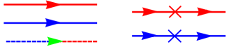
Figure 3: (Color online) Left panel: Feynman codex used for the representation of different Greens functions: blue (red) line (in the black and white printout the colors are different by intensity of gray (red is more intensive)) for Green function of even (odd) channel $G_{e(o)}$ and the mixed line for the mixed Green function $G_{eo}$ (see definition in Section IV.2.1). Right panel: two-particle elastic vertices for even and odd channels. Crosses denote energy-dependent scattering.

$$\hat{I}(x){=}{\frac{e}{2h\nu}}{\sum_{\sigma}}{\left[b^{\dagger}_{o\sigma}(x)b_{e\sigma}(x){-}b^{\dagger}_{o\sigma}({-}x)\mathcal{S}b_{e\sigma}({-}x)+\text{H.c.}\right]},$$ (19)

where $\mathcal{S}{=}S^{\ast}_{o}S_{e}$. There are two contributions to the charge current, coming from elastic and inelastic processes. The elastic effects are characterize by the energy-dependent phase-shifts, the inelastic ones are due to the interaction of Fermi-liquid quasi-particles. In the following section we outline the elastic and inelastic current contribution of two-stage Kondo model Eq. (12).

IV.1 Elastic current

We assume that the left and right scattering states are in thermal equilibrium at temperature $T_{L}{=}T_{R}{=}T$ and at the chemical potentials $\mu_{R}$ and $\mu_{L}{=}\mu_{R}{+}eV$. The population of states reads $2\langle b^{\dagger}_{ak\sigma}b_{ak^{\prime}\sigma}\rangle{=}\delta_{kk^{\prime}}\left[f_{L}(\varepsilon_{k}){+}f_{R}(\varepsilon_{k})\right]$ and $2\langle b^{\dagger}_{ak\sigma}b_{\bar{a}k^{\prime}\sigma}\rangle{=}\delta_{kk^{\prime}}\left[f_{L}(\varepsilon_{k}){-}f_{R}(\varepsilon_{k})\right]={}\delta_{kk^{\prime}}\Delta f(\varepsilon_{k})$ where $f_{L/R}(\varepsilon_{k}){=}f(\varepsilon_{k}{-}\mu_{L/R})$ and $f(\varepsilon_{k}){=}\left(1{+}\text{exp}\left[{\varepsilon_{k}}/{T}\right]\right)^{-1}$ is the Fermi-distribution function. The zero temperature conductance in the abscence of bias voltage is Pustilnik and Glazman (2004)

$$G(T=0,B\neq 0,V=0)/G_{0}=B^{2}\left(\alpha_{e}-\alpha_{o}\right)^{2}.$$

The elastic current in the absence of Zeeman field $B$ is the expectation value of the current operator Eq. (19). Taking the expectation value of Eq. (19) reproduces the Landauer-Büttiker equation Blanter and Nazarov (2009)

$$I_{\text{el}}=\frac{2e}{h}\int^{\infty}_{-\infty}d\varepsilon T(\varepsilon)\Delta f(\varepsilon),$$ (20)

where the energy dependent transmission coefficient, $T(\varepsilon){=}\frac{1}{2}\sum_{\sigma}\sin^{2}(\delta^{e}_{\sigma}(\varepsilon){-}\delta^{o}_{\sigma}(\varepsilon))$ and $\Delta f(\varepsilon){=}f_{L}(\varepsilon){-}f_{R}(\varepsilon)$. Diagrammatically (see Ref. Affleck and Ludwig (1993) and Ref. Hanl et al. (2014) for details), the elastic corrections to the current can be reabsorbed into a Taylor expansion for the energy-dependent phase shifts through the purely elastic contributions to quasi-particles self-energies Affleck and Ludwig (1993). That is the scattering phase-shifts can be read off Affleck and Ludwig (1993) via the real part of the retarded self-energies $\Sigma^{R}_{a,\sigma}(\varepsilon)$ (see Fig. 3) as

$$\delta^{a}_{\sigma}(\varepsilon){=}-\pi\nu\text{Re}\Sigma^{R}_{a,\sigma}(\varepsilon)=\pi/2+\alpha_{a}\varepsilon.$$ (21)

The Kondo temperatures of the two-channels in the strong-coupling limit are defined as

$$T_{K}^{a}=\frac{1}{\alpha_{a}}.$$ (22)

This definition is consistent with Nozieres-Blandin Nozieres and Blandin (1980) and identical to that used in Hanl et al. (2014), however, is differ by the coefficient $\pi/4$ from the spin-susceptibility based definition Filippone et al. (2017). The elastic phase-shifts in the presence of the finite Zeeman field $B$ bears the form Pustilnik and Glazman (2004) (see schematic behaviour of $\delta^{a}_{\downarrow}(B)$ in Fig. 4)

$$\delta^{a}_{\sigma}(B){=}\pi/2-(\alpha_{a}+\phi_{a}+\Phi)\bar{\sigma}B/2.$$ (23)

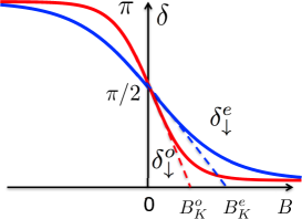
Figure 4: (Color online) Schematic behaviour of the even (blue) and odd (red) scattering phases at $\sigma=\downarrow$ as a function of the Zeeman magnetic field. Both phases approach the resonance value $\pi/2$ at zero field. The tangential lines illustrate corresponding energy scales inversely proportional to the spin susceptibilities (15) in the even/odd channels, $B_{K}^{a}=\pi/(2\alpha_{a}+\Phi)$ (see also Eqs.(21)-(23)).

Finally, we expand Eq. (20) up to second order in $\alpha_{a}$ to get the elastic contribution to the current Mora et al. (2008); Karki and Kiselev (2017),

$$\frac{I_{\text{el}}}{2e^{2}V/h}=\left[B^{2}+\frac{(eV)^{2}}{12}+\frac{(\pi T)^{2}}{3}\right](\alpha_{e}-\alpha_{o})^{2}.$$ (24)

The $B^{2}$ elastic term is attributed to the Zeeman field in Eq. (II). Note that we do not consider the orbital effects assuming that the magnetic field is applied parallel to the plane of the electron gas. The expression Eq. (24) remarkably highlights the absence of a linear response at $T{=}0$, $B{=}0$, due to the vanishing of conductance when both scattering phases achieve the resonance value $\pi/2$. The current is exactly zero at the symmetry point $\alpha_{e}{=}\alpha_{o}$ Pustilnik and Glazman (2004) due to the diagonal form of $S$-matrix characterized by two equal eigen values and therefore proportional to the unit matrix.

IV.2 Inelastic current

To calculate the inelastic contribution to the current we apply the perturbation theory using Keldysh formalism Keldysh (1965),

$$\delta I_{\text{in}}=\langle T_{C}\hat{I}(t)e^{-i\int dt^{\prime}H_{\text{int}}(t^{\prime})}\rangle,$$ (25)

where $H_{\text{int}}{=}H_{\phi}+H_{\Phi}$ and $C$ denotes the double-side $\eta{=}\pm$ Keldysh contour. Here $T_{C}$ is corresponding time-ordering operator. The average is performed with the Hamiltonian $H_{0}$. The effects associated with quadratic Hamiltonian $H_{\alpha}$ are already accounted in $I_{\text{el}}$. Therefore, to obtain the second-order correction to the inelastic current we proceed by considering $H_{\text{int}}{=}H_{\phi}+H_{\Phi}$, with the Feynman diagrammatic codex as shown in Fig. 5.

Figure 5: (Color online) Feynman diagrammatic codex used for the calculation of inelastic current. Blue (red) circles denote the density-density intra-channel interaction in even (odd) channel respectively (see Eq. 12). Green circle denotes the inter-channel spin-spin interaction Eq. 12.

The perturbative expansion of Eq. (25) in $(B,T,eV)\ll T_{K}^{\text{{\color[rgb]{0,0,0} o}}}$ starts with the second-order contribution Affleck and Ludwig (1993) and is illustrated by Feynman diagrams of four types (see Fig. 6). The type-1 and type-2 diagrams contain only one mixed Green’s function, GF (dashed line) proportional to $\Delta f(t){\sim}eV$, where $\Delta f(t)$ is the Fourier transform of $\Delta f(\varepsilon)$ defined in Eq. (75). Therefore, both diagrams fully define the linear-response contribution to the inelastic current, but also contain some non-linear ${\propto}(eV)^{3}$ contributions. The type-1 diagram contains the mixed GF directly connected to the current vertex (Fig. 6) and can be expressed in terms of single-particle self-energies. The type-2 diagram contains the mixed GF completely detached from the current vertex and therefore can not be absorbed into self-energies. We will refer to this topology of Feynman diagram as a vertex correction. Note, that the second-order Feynman diagrams containing two (and also four) mixed GF are forbidden due to PH symmetry of the problem. The type-3 and type-4 diagrams contain three mixed GF’s and therefore contribute only to the non-linear response being proportional to $(eV)^{3}$. The type-3 diagram, similarly to the type-1 diagram, can be absorbed into the single-particle self-energies. The type-4 diagram, similarly to the type-2 diagram is contributing to the vertex corrections. This classification can be straightforwardly extended to higher order perturbation corrections for the current operator. Moreover, the diagrammatic series will have similar structure also for the Hamiltonians without particle-hole symmetry where more vertices are needed to account for different types of interactions. A similar classification can also be done for current-current (noise) correlation functions Karki and Kiselev (2018).

$\underbrace{\includegraphics[height=62.59605pt]{y5.pdf}}_{\rm type\;1}\;\;\;\underbrace{\includegraphics[height=62.59605pt]{y11.pdf}}_{\rm type\;2}\linebreak\underbrace{\includegraphics[height=62.59605pt]{z10.pdf}}_{\rm type\;3}\;\;\;\underbrace{\includegraphics[height=62.59605pt]{z14.pdf}}_{\rm type\;4}$

Figure 6: (Color online) Examples of four different types of Feynamn diagrams contributing to the inelastic current. The open circle represents the current vertex. The other notations have been defined in Fig. 3 and Fig. 5.

The mathematical details of the computation of the diagrammatic contribution of current correction diagrams type-1, type-2, type-3 and type-4 as shown in Fig. 6 proceed as follows:

IV.2.1 Evaluation of type-1 diagram

The straightforward calculation of the Keldysh GFs at $x=0$ takes the form (see Refs. Mora et al. (2009); Karki and Kiselev (2017) for details)

$$G_{aa}(\varepsilon) =i\pi\nu\begin{bmatrix}F_{0}(\varepsilon)&F_{0}(\varepsilon)+1\\ F_{0}(\varepsilon)-1&F_{0}(\varepsilon)\end{bmatrix},$$

$$G_{aa}(\varepsilon) =i\pi\nu\begin{bmatrix}1&\phantom{-}1\\ 1&\phantom{-}1\end{bmatrix}\Delta f(\varepsilon),$$ (26)

where $F_{0}=f_{L}+f_{R}-1$ and we have neglected the principal part which does not contribute in the flat band model. The current contribution proportional to $\Phi^{2}$ corresponding to the diagram of type-1 as shown in Fig. 6 is given by Mora et al. (2009)

$$\delta I^{\Phi^{2}}_{\text{int}}=\frac{e}{\nu h}\sum_{\eta_{1},\eta_{2}}\eta_{1}\eta_{2}\times\mathcal{Y}_{1}^{\eta_{1},\eta_{2}},$$ (27)

with

$${\mathcal{Y}_{1}^{\eta_{1},\eta_{2}}}{=}{\int}{\frac{d\varepsilon}{2\pi}}\left[{i\mathcal{S}}{G^{+\eta_{1}}_{ee}(-x,\varepsilon)}{\Sigma^{\eta_{1}\eta_{2}}(\varepsilon)}{G^{\eta_{2}-}_{eo}(x,\varepsilon)}{+}{\text{c.c.}}\right],$$

where $\mathcal{S}=S^{*}_{o}S_{e}$, $\eta_{1/2}$ are the Keldysh branch indices which takes the value of $+$ or $-$. The self-energy $\Sigma^{\eta_{1}\eta_{2}}$ in real time is

$${\Sigma^{\eta_{1}\eta_{2}}(t)}{=}{\left(\frac{\Phi}{\pi\nu^{2}}\right)^{2}} {\sum_{k_{1},k_{2},k_{3}}}G^{\eta_{1}\eta_{2}}_{ee}(k_{1},t)$$

$$\times{G^{\eta_{2}\eta_{1}}_{ee}(k_{2},-t)}{G^{\eta_{1}\eta_{2}}_{ee}(k_{3},t)}.$$ (28)

Using Eq. (IV.2.1) we express the diagonal and mixed GFs in real space as

$$G^{\eta_{1}\eta_{2}}_{aa}(\alpha x,\varepsilon) =i\pi\nu e^{i\alpha\varepsilon x/v_{f}}\left[F_{0}+\begin{cases}\phantom{-}\eta_{1},&\text{if }\alpha=\phantom{-}1\\ -\eta_{2},&\text{if }\alpha=-1\\ \end{cases}\right],$$

$$G^{\eta_{1}\eta_{2}}_{a\bar{a}}(x,\varepsilon) =i\pi\nu e^{i\varepsilon x/v_{f}}\Delta f(\varepsilon),$$ (29)

The expression of corresponding GFs in real time is obtained by writing the Fourier transform of $\left(F_{0}(\varepsilon)\pm 1\right)$ as follows:

$$\int\frac{d\varepsilon}{2\pi}\left(F_{0}(\varepsilon)\pm 1\right)e^{-i\varepsilon t}$$

$$=\frac{i}{2\pi}\left[{\color[rgb]{0,0,0}\pm}\frac{\pi T}{\sinh(\pi Tt)}\left(e^{-i\mu_{L}t}+e^{-i\mu_{R}t}\right)-2\frac{e^{\pm iDt}}{t}\right].$$ (30)

Summing Eq. (27) over $\eta_{1}$ and $\eta_{2}$ using Eq. (IV.2.1) results two terms involving $\Sigma^{++}-\Sigma^{--}$ and $\Sigma^{-+}-\Sigma^{+-}$. First term produces the contribution which is proportional to model cut-off $D$ is eliminated by introducing the counter terms in the Hamiltonian Eq. (70). In rest of the calculation we consider only the contribution which remain finite for $D\rightarrow\infty$. As a result we get

$$\delta I^{\Phi^{2}}_{\text{int}}=\frac{2e\pi}{h}\int\frac{d\varepsilon}{2\pi}\left(\Sigma^{-+}(\varepsilon)-\Sigma^{+-}(\varepsilon)\right)i\pi\nu\Delta f(\varepsilon).$$ (31)

In Eq. (31) we used $\mathcal{S}+\mathcal{S}^{*}=2\cos(\delta^{e}_{0,\sigma}-\delta^{o}_{0,\sigma})=2$ with $\delta^{e}_{0,\sigma}{=}\delta^{o}_{0,\sigma}{=}\pi/2$. Fourier transformation of Eq. (31) into real time takes the form

$$\delta I^{\Phi^{2}}_{\text{int}}=\frac{2e\pi}{h}\int dt\left(\Sigma^{-+}(t)-\Sigma^{+-}(t)\right)i\pi\nu\Delta f(-t).$$ (32)

From Eq. (IV.2.1) the required Greens Function in real time are

$$G^{+-}_{ee}(t)=-\pi\nu T\frac{\cos(\frac{eV}{2}t)}{\sinh(\pi Tt)},$$ (33)

$$G_{eo}(t)=i\pi\nu T\frac{\sin(\frac{eV}{2}t)}{\sinh(\pi Tt)},$$ (34)

and $G^{-+}_{ee}(t)=G^{+-}_{ee}(-t)$. The self-energies in Eq. (32) are accessible by using above Greens functions Eq. (33) and Eq. (34) into self energy Eq. (IV.2.1). Then Eq. (32) results in

$$\delta I^{\Phi^{2}}_{\text{int}}{=}\frac{2e\pi}{h}\left(\frac{\phi_{e}}{\pi\nu^{2}}\right)^{2}\times 2i(\pi\nu T)^{4}\int dt\frac{\cos^{3}(\frac{eV}{2}t)\sin(\frac{eV}{2}t)}{\sinh^{4}(\pi Tt)}.$$ (35)

The integral Eq. (35) is calculated in Appendix E. Hence the interaction correction to the current corresponding to the type-1 diagrams shown in Fig. 6 is

$$\frac{\delta I^{\Phi^{2}}_{\text{type}-1}}{2e^{2}V/h}{=}\left[A^{(1)}_{V}(eV)^{2}+A^{(1)}_{T}(\pi T)^{2}\right]\Phi^{2},$$ (36)

where $A^{(1)}_{V}=5/12\;\text{and}\;A^{(1)}_{T}=2/3$. Alternatively, the calculation of the integral Eq. (31) can be proceed by scattering T-matrix formalism. The single particle self energy difference accociated with the diagram of type-1 is expressed in terms of inelastic T-matrix to obtain Karki and Kiselev (2017); Pustilnik and Glazman (2004)

$$\Sigma^{-+}(\varepsilon){-}\Sigma^{+-}(\varepsilon){=}\frac{\Phi^{2}}{i\pi\nu}\left[\frac{3}{4}(eV)^{2}{+}\varepsilon^{2}{+}(\pi T)^{2}\right].$$ (37)

Using this self-energy difference and following the same way as we computed elastic current in Appendix C, one easily get the final expression for the current correction contributed by the diagram of type-1.

IV.2.2 Evaluation of type-2 diagram

The diagrammatic contribution of the type-2 diagram shown in Fig. 6 proportional to $\phi_{e}\Phi$ given by

$$\delta I^{\phi_{e}\Phi}_{\text{int}}=\frac{e}{\nu h}\mathcal{J}=\frac{e}{\nu h}\sum_{\eta_{1},\eta_{2}}\eta_{1}\eta_{2}\mathcal{Y}_{2}^{\eta_{1},\eta_{2}},$$ (38)

with

$$\mathcal{Y}_{2}^{\eta_{1},\eta_{2}}{=}{\int}{\frac{d\varepsilon}{2\pi}}\left[{i\mathcal{S}}{G^{+\eta_{1}}_{ee}(-x,\varepsilon)}{\Lambda^{\eta_{1}\eta_{2}}_{1}(\varepsilon)}{G^{\eta_{2}-}_{oo}(x,\varepsilon)}{+\text{c.c.}}\right].$$

The self energy part $\Lambda_{1}$ in real time is expressed as

$$\Lambda^{\eta_{1}\eta_{2}}_{1}(t)=\frac{\phi_{e}\Phi}{(\pi\nu^{2})^{2}} \sum_{k_{1},k_{2},k_{3}}G^{\eta_{1}\eta_{2}}_{ee}(k_{1},t)$$

$$\times G^{\eta_{2}\eta_{1}}_{ee}(k_{2},-t)G^{\eta_{1}\eta_{2}}_{eo}(k_{3},t).$$ (39)

Now using Eq. (IV.2.1) into Eq. (38) followed by the summation over Keldysh indices, we get

$$\mathcal{J}=2i\mathcal{S}(\pi\nu)^{2} \int dt[(F_{0}+1)(t)\Lambda^{-+}_{1}(-t)$$

$$-(F_{0}-1)(t)\Lambda^{+-}_{1}(-t)]+\text{c.c.}$$ (40)

Let us define the Greens function as $G^{+-/-+}_{ee}(t)=G^{+-/-+}_{oo}(t)\equiv G^{+-/-+}(t)$. Then we write

$$i\pi\nu(F_{0}\pm 1)(t)=G^{+-/-+}(t),$$ (41)

where $(F_{0}\pm 1)(t)$ is a shorthand notation for the Fourier transform of $F_{0}(\varepsilon)\pm 1$ defined by (IV.2.1). Hence, Eq. (IV.2.2) takes the form

$$\mathcal{J}{=}{2\mathcal{S}\pi\nu}{\int}{dt}\left[{G^{+-}(t)}{\Lambda^{-+}_{1}({-t})}{-}{G^{-+}(t)}{\Lambda^{+-}_{1}({-t})}\right]{+\text{c.c.}}$$ (42)

Now the self energies in Eq. (IV.2.2) cast the compact form

$$\Lambda^{-+}_{1}(-t) =\frac{\phi_{e}\Phi}{(\pi\nu^{2})^{2}}G^{-+}(-t)G^{+-}(t)G_{eo}(-t).$$ (43)

$$\Lambda^{+-}_{1}(-t) =\frac{\phi_{e}\Phi}{(\pi\nu^{2})^{2}}G^{+-}(-t)G^{-+}(t)G_{eo}(-t).$$ (44)

Then the Eq. (42) becomes

$$\mathcal{J}=4\mathcal{S}\pi\nu\frac{\phi_{e}\Phi}{(\pi\nu^{2})^{2}}\int dt\left[G^{+-}(t)\right]^{3}G_{eo}(t)+\text{c.c.}$$ (45)

Using the explicit expressions of the Greens functions Eqs. (33) and  (34) together with Eq. (45) leads to

$$\mathcal{J}=-4i(\pi\nu)^{2}\mathcal{S}T(\pi\nu T)^{3}\frac{\phi_{e}\Phi}{(\pi\nu^{2})^{2}}\int dt\frac{\cos^{3}(\frac{eV}{2}t)\sin(\frac{eV}{2}t)}{\sinh^{4}(\pi Tt)}.$$ (46)

Substituting the value of integral given by Eq. (91) into Eq. (46) and using Eq. (38) we get

$$\frac{\delta I^{\phi_{e}\Phi}_{\text{type}-2}}{2e^{2}V/h}{=}\left[{A^{(2)}_{V}(eV)^{2}}{+}{A^{(2)}_{T}(\pi T)^{2}}\right]{\phi_{e}\Phi},$$ (47)

where $A^{(2)}_{V}=-5/6\;\text{and}\;A^{(2)}_{T}=-4/3.$

IV.2.3 Evaluation of type-3 diagram

Here we calculate the contribution to the current given by the diagram which consists of the self energy with two mixed Greens functions and one diagonal Greens function (type-3 diagram). The diagram shown in Fig. 6 describes correction proportional to $\phi_{e}\Phi$ and is given by

$$\delta I^{\phi_{e}\Phi}_{\text{int}}=\frac{e}{\nu h}\sum_{\eta_{1},\eta_{2}}\eta_{1}\eta_{2}\mathcal{Y}_{3}^{\eta_{1},\eta_{2}},$$ (48)

with

$${\mathcal{Y}_{3}^{\eta_{1},\eta_{2}}}{=}{\int}{\frac{d\varepsilon}{2\pi}}\left[i\mathcal{S}G^{+\eta_{1}}_{ee}({-}x,\varepsilon)\Lambda^{\eta_{1}\eta_{2}}_{2}(\varepsilon)G^{\eta_{2}-}_{eo}(x,\varepsilon){+}{\text{c.c.}}\right].$$

The self-energy $\Lambda^{\eta_{1}\eta_{2}}_{2}$ in real time is

$$\Lambda^{\eta_{1}\eta_{2}}_{2}(t)=\frac{\phi_{e}\Phi}{(\pi\nu^{2})^{2}} \sum_{k_{1},k_{2},k_{3}}G^{\eta_{1}\eta_{2}}_{eo}(k_{1},t)$$

$$\times G^{\eta_{2}\eta_{1}}_{oe}(k_{2},-t)G^{\eta_{1}\eta_{2}}_{ee}(k_{3},t).$$ (49)

Summing Eq. (48) over $\eta_{1}$ and $\eta_{2}$ using Eq. (IV.2.1), we get

$$\delta I^{\phi_{e}\Phi}_{\text{int}}{=}{\color[rgb]{0,0,0}-}\frac{e}{\nu h}\times\pi\nu\mathcal{S}\int\frac{d\varepsilon}{2\pi}\left(\Lambda^{-+}_{2}(\varepsilon)-\Lambda^{+-}_{2}(\varepsilon)\right)i\pi\nu\Delta f(\varepsilon)+\text{c.c.}$$ (50)

The Fourier transformation of Eq. (50) into real time gives

$$\delta I^{\phi_{e}\Phi}_{\text{int}}{=}{\color[rgb]{0,0,0}-}\frac{e}{\nu h}\times\pi\nu\mathcal{S}\int dt\left(\Lambda^{-+}_{2}(t)-\Lambda^{+-}_{2}(t)\right)i\pi\nu\Delta f(-t)+\text{c.c.}$$ (51)

Using the expressions of Greens functions in real time Eq. (33) and Eq. (34) allows to bring the interaction correction to the current Eq. (51) to a compact form

$$\begin{split}\delta I^{\phi_{e}\Phi}_{\text{int}}{=}{\color[rgb]{0,0,0}+}\frac{2e\pi}{h}{\times}2i(\pi\nu T)^{4}\frac{\phi_{e}\Phi}{(\pi\nu^{2})^{2}}{\int}dt\frac{\cos(\frac{eV}{2}t)\sin^{3}(\frac{eV}{2}t)}{\sinh^{4}(\pi Tt)}.\end{split}$$ (52)

Using Eq. (94) into Eq. (52) we get

$$\frac{\delta I^{\phi_{e}\Phi}_{\text{type}-3}}{2e^{2}V/h}{=}\left[A^{(3)}_{V}(eV)^{2}+A^{(3)}_{T}(\pi T)^{2}\right]\phi_{e}\Phi,$$

where $A^{(3)}_{V}={\color[rgb]{0,0,0}-}1/4\;\text{and}\;A^{(3)}_{T}=0.$

IV.2.4 Evaluation of type-4 diagram

In this Section we calculate the diagrammatic contribution of the $\phi_{e}\phi_{o}$ current diagrams (type-4 diagram) shown in Fig. 6. Similar to type-2 diagram calculation, the current correction reads

$$\delta I^{\phi_{e}\phi_{o}}_{\text{int}}=\frac{e}{\nu h}\mathcal{L}=\frac{e}{\nu h}\sum_{\eta_{1},\eta_{2}}\eta_{1}\eta_{2}\mathcal{Y}_{4}^{\eta_{1},\eta_{2}},$$ (53)

with

$$\mathcal{Y}_{4}^{\eta_{1},\eta_{2}}{=}{\int}\frac{d\varepsilon}{2\pi}\left[i\mathcal{S}G^{+\eta_{1}}_{ee}(-x,\varepsilon)\Lambda^{\eta_{1}\eta_{2}}_{3}(\varepsilon)G^{\eta_{2}-}_{oo}(x,\varepsilon){+}\text{c.c.}\right].$$ (54)

The self-energy part $\Lambda^{\eta_{1}\eta_{2}}_{3}$ is given by the expression

$$\Lambda^{\eta_{1}\eta_{2}}_{3}(t)=\frac{\phi_{e}\phi_{o}}{(\pi\nu^{2})^{2}} \sum_{k_{1},k_{2},k_{3}}G^{\eta_{1}\eta_{2}}_{oe}(k_{1},t)$$

$$\times G^{\eta_{2}\eta_{1}}_{eo}(k_{2},-t)G^{\eta_{1}\eta_{2}}_{eo}(k_{3},t).$$ (55)

Now substituting Eq. (IV.2.1) into Eq. (54) followed by the summation over Keldysh indices, we get

$$\mathcal{L}=2i\mathcal{S}(\pi\nu)^{2} \int dt[(F_{0}+1)(t)\Lambda^{-+}_{3}(-t)$$

$$-(F_{0}-1)(t)\Lambda^{+-}_{3}(-t)]+\text{c.c.}$$ (56)

Plugging in Eq. (41) into Eq. (IV.2.4) results

$$\mathcal{L}{=}2\mathcal{S}\pi\nu{\int}{dt}\left[G^{+-}(t)\Lambda^{-+}_{3}({-}t){-}G^{-+}(t)\Lambda^{+-}_{3}({-}t)\right]{+}\text{c.c.}$$ (57)

The self-energy Eq. (57) takes the form

$$\Lambda^{-+}_{3}(-t)=\frac{\phi_{e}\phi_{o}}{(\pi\nu^{2})^{2}}\left[G_{eo}(t)\right]^{3}=\Lambda^{+-}_{3}(-t).$$ (58)

Hence combining Eq. (33) and Eq. (34) we bring the required integral Eq. (57) to the form

$$\mathcal{L}={\color[rgb]{0,0,0}-}\frac{\phi_{e}\phi_{o}}{(\pi\nu^{2})^{2}}\times 4i\mathcal{S}\pi\nu(\pi\nu T)^{4}\int dt\frac{\cos(\frac{eV}{2}t)\sin^{3}(\frac{eV}{2}t)}{\sinh^{4}(\pi Tt)}+\text{c.c.}$$ (59)

The integral in Eq. (59) is given by Eq.(94). Hence plugging in Eq. (59) into Eq. (53) we obtain the current correction:

$$\frac{\delta I^{\phi_{e}\phi_{o}}_{\text{type}-4}}{2e^{2}V/h}{=}\left[A^{(4)}_{V}(eV)^{2}+A^{(4)}_{T}(\pi T)^{2}\right]\phi_{e}\phi_{o},$$ (60)

where $A^{(4)}_{V}={\color[rgb]{0,0,0}+}1/2\;\text{and}\;A^{(4)}_{T}=0$.

As we discussed above, all the current diagrams are of the form of type-1, type-2, type-3 and type-4. However, same type of diagrams may contain different numbers of fermionic loops and also different spin combinations. In addition, there is the renormalization factor of $-\frac{1}{2}$ in $H_{\Phi}$, which has to be accounted for the diagrams containing at least one $\Phi$ vertex. Same type of diagrams containing at least one $\Phi$ vertex with different spin combination have the different weight factor because of product of Pauli matrices in $H_{\Phi}$. Each fermionic loop in the diagrams results in extra $(-1)$ multiplier in the corresponding weight factor. These facts will be accounted for by assigning the weight to the given current diagram (e.g. as shown in Fig. 7, Fig. 8 and Fig. 9).

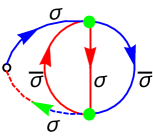
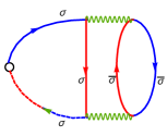
Figure 7: (Color online) The $\Phi^{2}$ type-1 diagram (Left panel) and the corresponding diagram with the splitting of local $\Phi$ vertices (Right panel). In the diagram the upper $\Phi$ vertex consist in the Pauli matrices product $\tau_{\sigma\bar{\sigma}}.\tau_{\bar{\sigma}\sigma}{=}2$. Similarly the lower $\Phi$ vertex contain the product of $\tau_{\bar{\sigma}\sigma}.\tau_{\sigma\bar{\sigma}}{=}2$. The diagram contains the even number of fermionic loops (two) and hence no extra negative sing occur due to the fermionic loop. Each $\Phi$ vertex has the renormalization factor of $-\frac{1}{2}$. Hence the overall weight factor of this diagram is $\frac{1}{4}{\times}4$ as will be seen in Fig. 11 and Fig. 12.

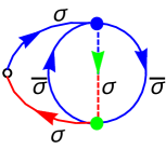
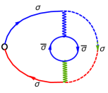
Figure 8: (Color online) The $\phi_{e}\Phi$ type-2 current correction diagram (Left panel) and the corresponding diagram with the splitting of local $\Phi$ vertices (Right panel). In the diagram the $\Phi$ vertex consist in the Pauli matrices product $\tau_{\sigma\sigma}.\tau_{\bar{\sigma}\bar{\sigma}}{=}-1$. The diagram contain the even number of fermionic loops (two) and hence no extra negative sing occur due to the fermionic loop. The $\Phi$ vertex has the renormalization factor of $-\frac{1}{2}$. Hence the overall weight factor of this diagram is $-\frac{1}{2}{\times}(-1)$ as will be seen in Fig. 11 and Fig. 12.

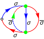
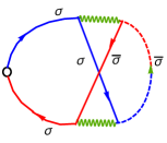
Figure 9: (Color online) The $\Phi^{2}$ type-2 current correction diagram (Left panel) and the corresponding diagram with the splitting of local $\Phi$ vertices (Right panel). In the diagram the upper $\Phi$ vertex consist in the Pauli matrices product $\tau_{\sigma\sigma}.\tau_{\bar{\sigma}\bar{\sigma}}{=}-1$. Similarly the lower $\Phi$ vertex contain the product of $\tau_{\bar{\sigma}\sigma}.\tau_{\sigma\bar{\sigma}}{=}2$. The diagram contain no fermionic loops and hence no extra negative sing occur due to the fermionic loop. Each $\Phi$ vertex has the renormalization factor of $-\frac{1}{2}$. Hence the overall weight factor of this diagram is $\frac{1}{4}{\times}(-2)$ as will be seen in Fig. 11 and Fig. 12

However, in these equations proper weight factors which emerge from (i) the number of closed fermionic loops, (ii) SU(2) algebra of Pauli matrices and (iii) additional factors originating from the definition of the FL constants in the Hamiltonian (the extra factor of $-1/2$ in $H_{\Phi}$) are still missing and are accounted for separately. As a result our final expression for the second-order perturbative interaction corrections to the current is given by (see Appendix D)

$$\frac{\delta I_{\text{in}}}{2e^{2}V/h} =\left[\frac{2}{3}(\phi^{2}_{e}+\phi^{2}_{o})+3\Phi^{2}-2(\phi_{e}+\phi_{o})\Phi\right](\pi T)^{2}$$

$$+\Big{[}\frac{5}{12}(\phi^{2}_{e}+\phi^{2}_{o})+{\color[rgb]{0,0,0}3}\Phi^{2}-{\color[rgb]{0,0,0}2}(\phi_{e}+\phi_{o})\Phi$$

$${\color[rgb]{0,0,0}+}\frac{1}{2}\phi_{e}\phi_{o}\Big{]}(eV)^{2}.$$ (61)

The first term $\propto(\pi T)^{2}$ in Eq. (IV.2.4) is the linear response result given by type-1 and type-2 diagrams. The second term (surviving also at $T=0$) is the non-linear response contribution arising from all type 1-4 diagrams. The inelastic current Eq. (IV.2.4) vanishes at the symmetry point. Moreover the linear response and the non-linear response contributions vanish at the symmetry point independently. Also the elastic and inelastic currents approach zero separately when the system is fine-tuned to the symmetry point. These properties will be reproduced in arbitrary order of perturbation theory.

V Transport properties

The total current consists of the sum of elastic and inelastic parts which upon using the FL-identity $\alpha_{a}{=}\phi_{a}$ takes the form

$$\frac{\delta I}{2e^{2}V/h} =\left[(\pi T)^{2}{\color[rgb]{0,0,0}+}(eV)^{2}\right]3(\Phi-\frac{2}{3}\alpha_{e})(\Phi-\frac{2}{3}\alpha_{o})$$

$$+\left[B^{2}+(\pi T)^{2}+\frac{1}{2}(eV)^{2}\right]\left(\alpha_{e}-\alpha_{o}\right)^{2}.$$ (62)

This Eq. (V) constitutes the main result of this work where the second term describes universal behaviour Pustilnik and Glazman (2004) scaled with $\left(1/T_{K}^{e}{-}1/T_{K}^{o}\right)^{2}$, while the first one, containing an extra dependence on the ratio $T_{K}^{o}/T_{K}^{e}$ accounts for the non-universality associated with the lack of conformal symmetry away from the symmetry-protected points. The Eq. (V) demonstrates the magnetic field $B$, temperature $T$ and voltage $V$ behaviour of the charge current characteristic for the Fermi-liquid systems. Therefore, following Hanl et al. (2014) we introduce general FL constants as follows:

$$\frac{1}{G_{0}}\frac{\partial I}{\partial V}=c_{B}B^{2}+c_{T}(\pi T)^{2}+c_{V}(eV)^{2}.$$ (63)

$$\frac{c_{T}}{c_{B}}=1+3\mathcal{F},\;\;\;\;\;\;\frac{c_{V}}{c_{B}}=\frac{{\color[rgb]{0,0,0}3}}{2}+{\color[rgb]{0,0,0}9}\mathcal{F}.$$ (64)

Here the parameter

$$\mathcal{F}=\frac{(\Phi-\frac{2}{3}\alpha_{e})(\Phi-\frac{2}{3}\alpha_{o})}{\left(\alpha_{e}-\alpha_{o}\right)^{2}}=\frac{4}{9}\frac{(\lambda_{eo}-\lambda_{e})(\lambda_{eo}-\lambda_{o})}{\left(\lambda_{e}-\lambda_{o}\right)^{2}}.$$ (65)

The parameter $\mathcal{F}$ vanishes in the limit of strong asymmetry, ${\color[rgb]{0,0,0}\lambda_{eo}{\ll}\lambda_{e}{\ll}\lambda_{o}}$ in which the ratios

$$\left.c_{T}/{c_{B}}\right|_{\color[rgb]{0,0,0}\lambda_{eo}\ll\lambda_{e}\ll\lambda_{o}}{=}1,\;\;\;\;\;\;\left.c_{V}/{c_{B}}\right|_{\color[rgb]{0,0,0}\lambda_{eo}\ll\lambda_{e}\ll\lambda_{o}}{=}3/2$$ (66)

correspond to the universality class of the single-channel Kondo model Pustilnik and Glazman (2001a, 2004).

On the other hand, near the symmetry point $\lambda_{e}{=}\lambda_{o}{=}\lambda_{eo}$, the function $\mathcal{F}$ evidently depends sensitively on the precise manner in which the symmetry point is approached. In fact, a priori it appears unclear whether $\mathcal{F}$ even reaches a well-defined value at this point. To clarify this, additional information on the parameters $\lambda_{e}$, $\lambda_{o}$ and $\lambda_{eo}$ is required.

In full generality, the three parameters $\lambda_{e}$, $\lambda_{o}$ and $\lambda_{eo}$ of the FL theory are independent from each other. Nonetheless, we are considering here a specific Hamiltonian Eq. (8) with only two independent parameters $J_{e}$ and $J_{o}$, which implies that $\lambda_{eo}$ is in fact a function of $\lambda_{e}$ and $\lambda_{o}$. Although the corresponding functional form is not known, it can be deduced in the vicinity of the symmetric point $\lambda_{e}{=}\lambda_{o}{=}\lambda_{eo}$ from the following argument: the obvious $e\leftrightarrow o$ symmetry imposes that the Wilson ratio $R{=}8/3$ is an extremum at the symmetric point (see Fig. 10), or else said, that its derivative with respect to the channel imbalance ratio $\lambda_{o}/\lambda_{e}$ vanishes. The only expression compatible with this requirement and the $e\leftrightarrow o$ symmetry is $\lambda_{eo}{=}(\lambda_{e}{+}\lambda_{o})/2$, valid in the immediate vicinity of the symmetry point. Inserting this dependence in Eq. (65) predicts $\lim_{\lambda_{e}\to\lambda_{o}}\mathcal{F}{=}-1/9$ at the symmetric point, and

$$\left.c_{T}/{c_{B}}\right|_{\color[rgb]{0,0,0}\lambda_{eo}=\lambda_{e}=\lambda_{o}}{=}2/3,\;\;\;\;\;\;\left.c_{V}/{c_{B}}\right|_{\color[rgb]{0,0,0}\lambda_{eo}=\lambda_{e}=\lambda_{o}}{=}{\color[rgb]{0,0,0}1/2}.$$ (67)

To summarize, under the assumption that the Wilson ratio is maximal at the symmetry point, we have arrived at the following conclusion: as the degree of asymmetry is reduced, i.e. the ratios ${\color[rgb]{0,0,0}\lambda_{e}/\lambda_{o}}$ and ${\color[rgb]{0,0,0}\lambda_{eo}/\lambda_{e}}$ increased from $0$ to $1$, the ratios of Fermi liquid coefficients $c_{T}/{c_{B}}$ and $c_{V}/{c_{B}}$ decrease from the maximal values of Eq. (66), to the minimal values of Eq. (67), characteristic of the 1CK and 2SK fixed points, respectively.

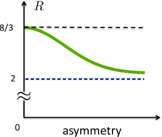
Figure 10: (Color online) Cartoon sketching the evolution of the Wilson ratio as a function of increasing “asymmetry”, meaning that the ratios $\lambda_{e}/\lambda_{o}$ and $\lambda_{eo}/\lambda_{e}$ both decrease from 1 at the left to 0 at the right. When $\lambda_{e}{=}\lambda_{o}{=}\lambda_{eo}$, meaning that the even and odd Kondo temperatures coincide, the total spin current is conserved Affleck and Ludwig (1993) and $R{=}8/3$ Affleck (1995). In the limit of extremely (exponentially) strong channel asymmetry of 2SK model, the (C) regime shown on Fig. 1 shrinks to zero. As a result, the 1CK universality class appears and Wilson Ratio is $R{=}2$ Affleck (1995). The behaviour of the Wilson ratio between these to limits is presumably monotonic, since the 2SK model has no other strong coupling fixed points.

VI Discussion

We constructed a Fermi-liquid theory of a two-channel, two-stage Kondo model when both scattering channels are close to the resonance. This theory completely describes the transport in in- and out-of-equilibrium situation of the 2SK model. The elastic and inelastic contributions to the charge current through the 2SK model have been calculated using the full-fledged non-equilibrium Keldysh formalism for arbitrary relation between two Kondo energy scales. While computing the current correction, we performed the full classification of the Feynman diagrams for the many-body perturbation theory on the Keldysh contour. We demonstrated the cancellation of the charge current at the symmetry protected point. The linear response and beyond linear response contributions to the current vanish separately at the symmetry point. Moreover, the independent cancellation of the elastic and inelastic currents at the symmetry protected point was verified. The theoretical method developed in the paper provides a tool for both quantitative and qualitative description of charge transport in the framework of the two-stage Kondo problem. In particular, the two ratios of FL constants, $c_{T}/c_{B}$ and $c_{V}/c_{B}$, quantify the “amount” of interaction between two channels. The interaction is strongest at the symmetry protected point due to strong coupling of the channels. The interaction is weakest at single-channel Kondo limit where the odd channel is completely decoupled from the even channel. While we illustrated the general theory of two resonance scattering channels by the two-stage Kondo problem, the formalism discussed in the paper is applicable for a broad class of models describing quantum transport through nano-structures Bauer et al. (2013); Heyder et al. (2015); Rejec and Meir (2006) and behaviour of strongly correlated systems Coleman (2015).

As an outlook, the approach presented in this paper can be applied to the calculation of current-current correlation functions (charge noise) of the 2SK problem and, by computing higher cumulants of the current, to studying the full-counting statistics Levitov and Lesovik (1993); Levitov (2003). It is straightforward to extend the presented ideas for generic Anderson-type models away from the particle-hole symmetric point Oguri and Hewson (2017, 2018a, 2018b), and generalize it for the SU(N) Kondo impurity Karki and Kiselev (2017) and multi-terminal (multi-stage) as well as multi-dot setup. The general method developed in the paper is not limited by its application to charge transport through quantum impurity — it can be equally applied to detailed description of the thermo-electric phenomena on the nano-scale Karki and Kiselev (2017).

Appendix A Overview of flow from weak to strong coupling

A.1 Weak coupling regime

We assume that at sufficiently high temperatures (a precise definition of this condition is given below) the even and odd channels do not talk to each other. As a consequence, we renormalise the coupling between channels and impurity spins ignoring the cross-channel interaction. Performing Anderson’s poor man’s scaling procedure Anderson (1970) to the even and odd channels independently we obtain the system of two decoupled renormalization group (RG) equations:

$$\frac{dJ_{e}}{d\Lambda}=2N_{F}J^{2}_{e},\quad\frac{dJ_{o}}{d\Lambda}=2N_{F}J^{2}_{o},$$ (68)

where $N_{F}$ is the 3D-density of states in the leads. The parameter $\Lambda{=}\ln\left(\frac{D}{\varepsilon}\right)$ depends on the ultraviolet cutoff of the problem (conduction bandwidth $D$). Note that the RG Eqs. (68) are decoupled only in one-loop approximation (equivalent to a summation of so-called parquet diagrams). The solution of these RG equations defines two characteristic energy scales, namely $T_{K}^{a}{=}D\exp\left(-1/(2N_{F}J_{a})\right)$, which are the Kondo temperatures in the even and odd channels respectively. The second loop corrections to RG couple the equations, generating the cross-term $\propto-J_{eo}\;\mathbf{s}_{e}\cdot\mathbf{s}_{o}$ with $J_{eo}\sim N_{F}J_{e}\cdot J_{o}$. This emergent term flows under RG and becomes one of the leading irrelevant operators of the strong coupling fixed point (the others are $:\mathbf{s}_{e}\cdot\mathbf{s}_{e}:$ and $:\mathbf{s}_{o}\cdot\mathbf{s}_{o}:$, see Eq.10). In addition, the second-loop corrections to RG lead to a renormalization of the pre-exponential factor in the definition of the Kondo temperatures.

Summarizing, we see that the $S{=}1$, ${\cal K}{=}2$ fully screened Kondo model has a unique strong coupling fixed point, where couplings $J_{e}$ and $J_{o}$ diverge in the RG flow. This strong coupling fixed point falls into the FL universality class. The weak coupling regime is therefore defined as $(B,T,eV){\gg}(T_{K}^{e},T_{K}^{o})$. Since the interaction between the even channel and local impurity spin corresponds to the maximal eigenvalue of the matrix Eq. (7), we will assume below that the condition $T_{K}^{e}{\geqslant}T_{K}^{o}$ holds for any given $B,T$ and $eV$ and, we thus define $T^{\text{min}}_{K}{=}T^{o}_{K}$. The differential conductance decreases monotonically with increasing temperature in the weak-coupling regime (see Fig. 1) being fully described by the perturbation theory Pustilnik and Glazman (2004) in $[1/\ln(T/T_{K}^{e}),1/\ln(T/T_{K}^{e})]\ll 1$.

A.2 Intermediate coupling regime

Next we consider the intermediate coupling regime $T_{K}^{o}{\leqslant}(B,T,eV){\leqslant}T_{K}^{e}$ depicted as the characteristic hump in Fig. 1. Since the solution of one-loop RG Eqs. (68) is given with logarithmic accuracy, we assume without loss of generality that $T_{K}^{e}$ and $T_{K}^{o}$ are of the same order of magnitude unless a very strong (exponential) channel asymmetry is considered. Therefore, the “hump regime” is typically very small and the hump does not have enough room to be formed. The intermediate regime is characterized by an incomplete screening (see Fig. 1) when one conduction channels (even) falls into a strong coupling regime while the other channel (odd) still remains at the weak coupling. Then the strong-coupling Hamiltonian for the even channel is derived along the lines of Affleck-Ludwig paper Ref. Affleck and Ludwig (1993) and is given by:

$$H_{\rm even} {=}H^{e}_{0}{+}\frac{3}{2}\lambda_{e}\rho_{e\uparrow}\rho_{e\downarrow}{-}\frac{3}{4v_{F}}\lambda_{e}\sum_{kk^{\prime}\sigma}\left(\varepsilon_{k}+\varepsilon_{k}^{\prime}\right)b^{\dagger}_{ek\sigma}b_{ek^{\prime}\sigma},$$ (69)

where the $b$-operators describe Fermi-liquid excitations, $\rho_{e\sigma}(x{=}0){=}\sum_{kk^{\prime}}b^{\dagger}_{ek\sigma}b^{\phantom{\dagger}}_{ek^{\prime}\sigma}$ and $\lambda_{e}\propto 1/T_{K}^{e}$ is the leading irrelevant coupling constant Affleck and Ludwig (1993).

The weak-coupling part of the remaining Hamiltonian is described by a $s_{\rm imp}{=}1/2$ Kondo-impurity Hamiltonian $H_{\rm odd}{=}J_{o}{\textbf{s}}_{o}\cdot{\textbf{s}}_{\rm imp}$. Here we have already taken into account that the impurity spin is partially screened by the even channel during the first stage process of the Kondo effect. We remind that the coupling between the even and odd channels is facilitated by a ferromagnetic interaction which emerges, being however irrelevant in the intermediate coupling regime. Thus, the differential conductance does reach a maximum $G/G_{0}{\approx}1$ with a characteristic hump Pustilnik and Glazman (2001a), Posazhennikova et al. (2007) at the intermediate coupling regime. Corresponding corrections (deviation of the conductance at the top of the hump from the unitary limit $G_{0}{=}2e^{2}/h$) can be calculated with logarithmic accuracy $|\delta G/G_{0}|{\propto}1/\ln^{2}(T_{K}^{e}/T_{K}^{o})$ Nozieres and Blandin (1980), Anderson (1970) (see also review Pustilnik and Glazman (2004) and Posazhennikova et al. (2007) for details).

Appendix B Counterterms

We proceed with the calculation of the corrections to the current by eliminating the dependence on the cutoff parameter $D$ by adding the counter terms in the Hamiltonian Affleck and Ludwig (1993); Mora et al. (2009)

$$H_{c}=-\frac{1}{2\pi\nu}\sum_{a}\sum_{kk^{\prime}\sigma}\left(\delta\alpha_{a}+\delta\Phi\right)(\varepsilon_{k}+\varepsilon_{k^{\prime}}):b^{\dagger}_{ak\sigma}b_{ak^{\prime}\sigma}:,$$ (70)

so that we consider only the contribution which remain finite for $D{\rightarrow}\infty$. The Eq. (70) corresponds to the renormalization of leading irrelevant coupling constant $\alpha_{a}$ such that $\alpha_{a}\rightarrow\alpha_{a}+\delta\alpha_{a}+\delta\Phi$ with

$$\delta\alpha_{a}= -\alpha_{a}\phi_{a}\frac{6D}{\pi}\log\left(\frac{4}{3}\right).$$ (71)

$$\delta\Phi= -\Phi^{2}\frac{9D}{\pi}\log\left(\frac{4}{3}\right).$$ (72)

During the calculation of the interaction correction we neglected those terms which produce the contribution proportional to the cutoff $D$ [for example, $\propto\int\frac{d\varepsilon}{2\pi}\left(\Sigma^{++}(\varepsilon)-\Sigma^{--}(\varepsilon)\right)i\pi\nu\Delta f(\varepsilon)$]. This renormalization of leading irrelevant coupling constant Eq. (70) exactly cancel these terms.

Appendix C Elastic current

To get the elastic current Eq. (24), we start from the Landauer-Büttiker formula Eq. (20)

$$I_{\text{el}}=\frac{2e}{h}\int_{-\infty}^{\infty}d\varepsilon T(\varepsilon)\Delta f(\varepsilon),$$ (73)

where the energy dependent transmission coefficient, $T(\varepsilon){=}\frac{1}{2}\sum_{\sigma}\sin^{2}(\delta^{e}_{\sigma}(\varepsilon)-\delta^{o}_{\sigma}(\varepsilon))$ and $\Delta f(\varepsilon){=}f_{L}(\varepsilon)-f_{R}(\varepsilon)$. Taylor expanding the phase shifts to the first order in energy and retaining only upto second order in energy terms in the $T(\varepsilon)$, we arrive at the expression

$$I_{\text{el}}=\frac{2e}{h}(\alpha_{e}-\alpha_{o})^{2}\int_{-\infty}^{\infty}d\varepsilon\varepsilon^{2}\Delta f(\varepsilon).$$ (74)

To compute the integral Eq. (74) we use the property of the Fourier transform. For the given function $\Delta f(\varepsilon)$, it’s Fourier transform is defined as

$$\Delta f(t)=\frac{1}{2\pi}\int_{-\infty}^{\infty}e^{-i\varepsilon t}\Delta f(\varepsilon)d\varepsilon.$$ (75)

Taking $n$-th derivative of Eq. (75) at $t=0$ we get

$$\int_{-\infty}^{\infty}\varepsilon^{n}\Delta f(\varepsilon)d\varepsilon=\frac{2\pi}{(-i)^{n}}\left.\partial_{t}^{n}\left[\Delta f(t)\right]\right|_{{}_{t=0}}.$$ (76)

Substituting Eq. (76) for $n=2$ into Eq. (74), the elastic current cast into the form

$$I_{\text{el}}=\frac{2e}{h}(\alpha_{e}-\alpha_{o})^{2}(-2\pi)\left.\partial_{t}^{2}\left[\Delta f(t)\right]\right|_{{}_{t=0}}.$$ (77)

The Fourier transform of $\Delta f(\varepsilon)$ for $\mu_{L/R}=\pm eV/2$ is defined by

$$\Delta f(t)=T\frac{\sin(\frac{eVt}{2})}{\sinh(\pi Tt)}.$$ (78)

Using Eq. (78) into Eq.(77), we can easily arrive at the expression Eq. (24) for the elastic current at finite temperature $T$, finite bias voltage $V$ and finite in-plane (Zeeman) magnetic field $B$ (assuming $(T,eV,B)\ll T_{K}^{o}$)

$$\frac{I_{\text{el}}}{2e^{2}V/h}=\left[B^{2}+\frac{(eV)^{2}}{12}+\frac{(\pi T)^{2}}{3}\right](\alpha_{e}-\alpha_{o})^{2}.$$ (79)

Appendix D Net electric current

Here we present the detail of the computation of total electric current (sum of elastic and inelastic parts) given by Eq. (V). We discuss the total current in linear-response (LR) and beyond linear-response (BLR) regime separately. The elastic part is given by Eq. (24) and the inelastic part which is composed of the four types of diagrams is expressed by Eq. (IV.2.4).

D.1 Linear Response (LR)

As discussed in the main text, both elastic and inelastic processes contribute to the LR current. The LR contribution of the elastic part is expressed by Eq. (24). The diagrams of type-1 and type-2 has the finite linear response contribution to the inelastic current. As detailed in Fig. 11, we have the expression of total linear response current

$$\frac{\delta I^{\text{LR}}}{2e^{2}V/h}\frac{1}{(\pi T)^{2}}=\Big{[}\underbrace{\frac{1}{3}\left(\alpha_{e}-\alpha_{o}\right)^{2}}_{\rm\text{LR elastic part}}\Big{]}+$$

$$\Big{[}\underbrace{A^{(1)}_{T}(\phi^{2}_{e}{+}\phi^{2}_{o}){+}3A^{(1)}_{T}\Phi^{2}{+}\frac{3A^{(2)}_{T}}{2}(\phi_{e}{+}\phi_{o})\Phi{-}\frac{3A^{(2)}_{T}}{4}\Phi^{2}}_{\rm\text{LR inelastic part (type-1 and type-2 diagrams)}}\Big{]}$$

$${=}\left[\frac{1}{3}\left(\alpha_{e}{-}\alpha_{o}\right)^{2}{+}\frac{2}{3}(\phi^{2}_{e}{+}\phi^{2}_{o}){-}2(\phi_{e}{+}\phi_{o})\Phi{+}3\Phi^{2}\right]$$

$${=}\left[(\alpha_{e}-\alpha_{o})^{2}+3(\Phi-\frac{2}{3}\alpha_{e})(\Phi-\frac{2}{3}\alpha_{o})\right].$$ (80)

At the symmetry point the linear response contribution to the current given by the Eq. (D.1) exactly vanishes.

$$\begin{split}\delta I^{\phi^{2}}_{\rm in}&=\phantom{-}\phantom{-}\left[\underbrace{\includegraphics[width=51.21504pt,valign={c}]{y1.pdf}}_{\rm type-1}\right]+\delta I^{\phi^{2}_{o}}_{\rm in}\\ &=\frac{2e^{2}V}{h}\left[A^{(1)}_{V}(eV)^{2}+A^{(1)}_{T}(\pi T)^{2}\right]\left(\phi^{2}_{e}+\phi^{2}_{o}\right)\\ \delta I^{\Phi^{2}}_{\rm in}&=+\frac{1}{4}\left[\underbrace{\phantom{-}\includegraphics[width=45.52458pt,valign={c}]{y2.pdf}+\includegraphics[width=45.52458pt,valign={c}]{y3.pdf}+\includegraphics[width=45.52458pt,valign={c}]{y4.pdf}}_{\rm\text{type-1}}\right]\\ &\phantom{-}+\frac{1}{4}\left[\underbrace{\includegraphics[width=45.52458pt,valign={c}]{y5.pdf}+4\includegraphics[width=45.52458pt,valign={c}]{y6.pdf}+4\includegraphics[width=45.52458pt,valign={c}]{y7.pdf}}_{\rm\text{type-1}}\right]\\ &\phantom{-}+\frac{1}{4}\left[\underbrace{\includegraphics[width=45.52458pt,valign={c}]{y8.pdf}-2\includegraphics[width=45.52458pt,valign={c}]{y9.pdf}-2\includegraphics[width=45.52458pt,valign={c}]{y10.pdf}}_{\rm\text{type-2}}\right]\\ &=\frac{6e^{2}V}{h}\Big{[}({A^{(1)}_{V}}{-}\frac{A^{(2)}_{V}}{4}){(}eV{)}^{2}{+}(A^{(1)}_{T}{-}\frac{A^{(2)}_{T}}{4})(\pi T)^{2}\Big{]}\Phi^{2}\\ \delta I^{\phi_{a}\Phi}_{\rm in}&={-}\frac{1}{2}\left[\underbrace{-\includegraphics[width=48.36958pt,valign={c}]{y11.pdf}-2\includegraphics[width=48.36958pt,valign={c}]{y12.pdf}}_{\rm\text{type-2 }}\right]+\delta I^{\phi_{o}\Phi}_{\rm in}\\ &=\frac{3e^{2}V}{h}\left[A^{(2)}_{V}(eV)^{2}+A^{(2)}_{T}(\pi T)^{2}\right]\left(\phi_{e}+\phi_{o}\right)\Phi\end{split}$$

Figure 11: (Color online) Feynman diagrams of type-1 and type-2 contributing to the charge current both in the linear response and beyond the linear response regime. The coefficients computed in the Sec IV.2.1 and Sec IV.2.2 take the following values: $A^{(1)}_{T}{=}2/3$, $A^{(2)}_{T}{=}-4/3$, $A^{(1)}_{V}{=}5/12$, $A^{(2)}_{V}{=}-5/6$.

D.2 Beyond Linear Response (BLR)

$$\begin{split}\delta I^{\Phi^{2}}_{\rm in}&{=}\phantom{-}\frac{1}{4}\left[\underbrace{\phantom{-}\includegraphics[width=48.36958pt,valign={c}]{z1.pdf}{+}\phantom{-}\includegraphics[width=48.36958pt,valign={c}]{z2.pdf}{+}4\includegraphics[width=48.36958pt,valign={c}]{z3.pdf}}_{\rm\text{type-4}}\right]\\ &\phantom{-}{+}\frac{1}{4}\left[\underbrace{\phantom{-}\includegraphics[width=48.36958pt,valign={c}]{z4.pdf}{+}\phantom{-}\includegraphics[width=48.36958pt,valign={c}]{z5.pdf}{-}2\includegraphics[width=48.36958pt,valign={c}]{z6.pdf}}_{\rm\text{type-3}}\right]\\ &\phantom{-}{+}\frac{1}{4}\left[\underbrace{-2\includegraphics[width=48.36958pt,valign={c}]{z7.pdf}{-}2\includegraphics[width=48.36958pt,valign={c}]{z8.pdf}{-}2\includegraphics[width=48.36958pt,valign={c}]{z9.pdf}}_{\rm\text{type-3}}\right]\\ &{=}\frac{3e^{2}V}{h}\left[(A^{(4)}_{V}{-}A^{(3)}_{V})(eV)^{2}+(A^{(4)}_{T}{-}A^{(3)}_{T})(\pi T)^{2}\right]{\Phi^{2}}\\ \delta I^{\phi_{a}\Phi}_{\rm in}&{=}{-}\frac{1}{2}\left[\underbrace{{-}\includegraphics[width=51.21504pt,valign={c}]{z10.pdf}{-}\includegraphics[width=51.21504pt,valign={c}]{z11.pdf}}_{\rm\text{type-3}}\right.\\ &\;\;\;\;\;\;\;\;\left.\underbrace{{-}2\includegraphics[width=51.21504pt,valign={c}]{z12.pdf}{-}2\includegraphics[width=51.21504pt,valign={c}]{z13.pdf}}_{\rm\text{type-3}}\right]+\delta I^{\phi_{o}\Phi}_{\rm in}\\ &{=}\frac{6e^{2}V}{h}\left[A^{(3)}_{V}(eV)^{2}{+}A^{(3)}_{T}(\pi T)^{2}\right]\left(\phi_{e}+\phi_{o}\right)\Phi\\ \delta I^{\phi_{e}\phi_{o}}_{\rm in}&{=}\left[\underbrace{\includegraphics[width=45.52458pt,valign={c}]{z14.pdf}}_{\rm type-4}\right]{=}\frac{2e^{2}V}{h}\left[A^{(4)}_{V}(eV)^{2}{+}A^{(4)}_{T}(\pi T)^{2}\right]\phi_{e}\phi_{o}\end{split}$$

Figure 12: (Color online) Feynman diagrams of type-3 and type-4 contributing to the charge current beyond the linear response. The coefficients computed in the Sec IV.2.3 and Sec IV.2.4 take the following values: $A^{(3)}_{T}{=}A^{(4)}_{T}{=}0$, $A^{(3)}_{V}{=}{\color[rgb]{0,0,0}-}1/4$, $A^{(4)}_{V}{=}{\color[rgb]{0,0,0}1/2}$.

The BLR contribution of the elastic part is expressed by Eq. (24). The diagrams of type-3 and type-4 produce the finite contribution to the inelastic current only beyond the LR regime. In addition to the LR contribution, the type-1 and type-2 diagrams also contribute to non-linear response. As detailed in Fig. 12, the total non-linear current is

$$\frac{\delta I^{\text{BLR}}}{2e^{2}V/h}\frac{1}{(eV)^{2}}=\Big{[}\underbrace{\frac{1}{12}\left(\alpha_{e}-\alpha_{o}\right)^{2}}_{\rm\text{BLR elastic part}}\Big{]}$$

$${+}{\left[\underbrace{A^{(1)}_{V}(\phi^{2}_{e}{+}\phi^{2}_{o}){+}3A^{(1)}_{V}\Phi^{2}{+}\frac{3A^{(2)}_{V}}{2}(\phi_{e}{+}\phi_{o})\Phi{-}\frac{3A^{(2)}_{V}}{4}\Phi^{2}}_{\rm\text{BLR inelastic part (type-1 and type-2 diagrams)}}\right]}$$

$${+}{\left[\underbrace{A^{(4)}_{V}\phi_{e}\phi_{o}+3A^{(3)}_{V}\left(\phi_{e}+\phi_{o}\right)\Phi+\frac{3}{2}(A^{(4)}_{V}-A^{(3)}_{V})\Phi^{2}}_{\rm\text{BLR inelastic part (type-3 and type-4 diagrams)}}\right]}$$

$${=}{\Big{[}\frac{1}{12}\left(\alpha_{e}-\alpha_{o}\right)^{2}+\frac{5}{12}(\phi^{2}_{e}+\phi^{2}_{o})-\frac{5}{4}(\phi_{e}+\phi_{o})\Phi}$$

$$\phantom{-}\phantom{-}{+\frac{15}{8}\Phi^{2}{\color[rgb]{0,0,0}+}\frac{1}{2}\phi_{e}\phi_{o}{\color[rgb]{0,0,0}-}\frac{3}{4}\left(\phi_{e}+\phi_{o}\right)\Phi{\color[rgb]{0,0,0}+}\frac{9}{8}\Phi^{2}}\Big{]}$$

$$={\color[rgb]{0,0,0}\left[\frac{1}{2}(\alpha_{e}-\alpha_{o})^{2}+3(\Phi-\frac{2}{3}\alpha_{e})(\Phi-\frac{2}{3}\alpha_{o})\right].}$$ (81)

The BLR contribution to the current expressed by Eq. (D.2) goes to zero at the symmetry point $\alpha_{e}{=}\alpha_{o}{=}3\Phi/2$.

The sum of the LR and BLR contributions results in Eq. (V). For completeness

$$\frac{\delta I}{2e^{2}V/h}=3 \left[(\pi T)^{2}{\color[rgb]{0,0,0}+}(eV)^{2}\right](\Phi-\frac{2}{3}\alpha_{e})(\Phi-\frac{2}{3}\alpha_{o})$$

$$+ \left[(\pi T)^{2}+\frac{1}{2}(eV)^{2}\right]\left(\alpha_{e}-\alpha_{o}\right)^{2}.$$ (82)

This equation represents in a simple and transparent form contribution of the three FL constants to the charge transport.

Appendix E Calculation of integrals

In this section we calculate two integrals that we used for the calculation of current correction contributed by four types of diagram. The first integral to calculate is

$$\mathcal{I}_{1}=\int^{\infty}_{-\infty}\frac{\cos^{3}(\frac{eV}{2}t)\sin(\frac{eV}{2}t)}{\sinh^{4}(\pi Tt)}dt.$$ (83)

The singularity of the integral in Eq. (83) is removed by shifting the time contour by $i\gamma$ in the complex plane as shown in Fig. 13. The point splitting parameter $\gamma$ is chosen to satisfy the conditions $\gamma$$D$$\gg 1$ and $\gamma$$T$$\ll 1$, $\gamma$$e$$V$$\ll 1$, where, $D$ is the band cutoff. Then the Eq.(83) can be written as

$$\begin{split}&\mathcal{I}^{+}_{1}=\int^{\infty+i\gamma}_{-\infty+i\gamma}\frac{\cos^{3}(at)\sin(at)}{\sinh^{4}(\pi Tt)}dt\\ &{=}{-}\frac{i}{16}{\left[\mathcal{Z}(4a,T){-}\mathcal{Z}({-}4a,T)+2\mathcal{Z}(2a,T){-}2\mathcal{Z}({-}2a,T)\right]}.\end{split}$$ (84)

In Eq. (84), $a{=}eV/2$ and we introduced the short hand notation,

$$\mathcal{Z}(a,T){=}\int^{\infty+i\gamma}_{-\infty+i\gamma}\frac{e^{iat}}{\sinh^{4}(\pi Tt)}dt{=}\int^{\infty+i\gamma}_{-\infty+i\gamma}h(a,T;t)dt.$$ (85)

The poles of the integrand $h(a,T;t)$ in Eq. (85) are

$$\pi Tt=\pm im\pi\Rightarrow t=\pm\frac{im}{T},\quad m=0,\pm 1,\pm 2,\pm 3...$$ (86)

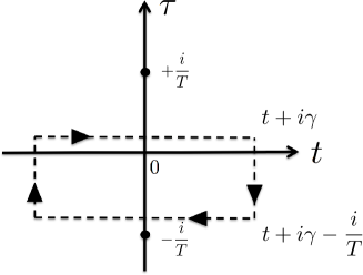
Figure 13: The contour of the integration for the integral Eq. (83) with negative shift.

The integration of $h(a,T;t)$ over the rectangular contour Fig. 13 shifted by $i/T$ upon using the Cauchy residue theorem results

$$\begin{split}\mathcal{Z}(a,T)&=\int^{\infty+i\gamma}_{-\infty+i\gamma}\frac{e^{ia(t-\frac{i}{T})}}{\sinh^{4}\left(\pi T(t-\frac{i}{T})\right)}dt\\ &-2\pi i\times\left.\text{\text{Res}}[h(a,T;t)]\right|_{t=0},\end{split}$$ (87)

where “Res” stands for the residue. By expanding the $\sinh$ function in Eq .(87) we get

$$\mathcal{Z}(a,T)\left(1-e^{\frac{a}{T}}\right)=-2\pi i\times\left.\text{Res}[h(a,T;t)]\right|_{t=0}.$$ (88)

By using the standard formula for the calculation of the residue, Eq. (88) cast the form

$$\mathcal{Z}(a,T)=-\frac{2\pi\left(a^{3}+4a(\pi T)^{2}\right)}{6(\pi T)^{4}}\times\frac{1}{1-e^{\frac{a}{T}}}.$$ (89)

Use of Eq. (89) into Eq. (84) gives the required integral

$$\mathcal{I}^{+}_{1} =\frac{i\pi}{(\pi T)^{4}}\frac{eV}{2}\left[\frac{5}{12}(eV)^{2}+\frac{2}{3}(\pi T)^{2}\right].$$ (90)

Choosing the contour with the negative shift results in the integral $\mathcal{I}^{-}_{1}$ such that $\mathcal{I}^{-}_{1}{=}-\mathcal{I}^{+}_{1}$. As a result

$$\mathcal{I}^{\pm}_{1}(V,T) =\pm\frac{i\pi}{(\pi T)^{4}}\frac{eV}{2}\left[\frac{5}{12}(eV)^{2}+\frac{2}{3}(\pi T)^{2}\right].$$ (91)

The second integral that we are going to compute is

$$\mathcal{I}_{2}=\int^{\infty}_{-\infty}\frac{\cos(\frac{eV}{2}t)\sin^{3}(\frac{eV}{2}t)}{\sinh^{4}(\pi Tt)}dt.$$ (92)

In the same way and using the same notations as for the first integral, Eq. (92) reads

$$\mathcal{I}^{+}_{2} {=}\frac{i}{16}{\left[\mathcal{Z}(4a,T){-}\mathcal{Z}({-}4a,T){-}2\mathcal{Z}(2a,T){+}2\mathcal{Z}({-}2a,T)\right]}$$

$${=}{-}\frac{i\pi}{(\pi T)^{4}}\left(\frac{eV}{2}\right)^{3}.$$ (93)

Similar to Eq. (91), the integral $\mathcal{I}_{2}$ takes the form

$$\mathcal{I}^{\pm}_{2}(V,T)=\mp{\frac{i\pi}{(\pi T)^{4}}}{\left(\frac{eV}{2}\right)^{3}}.$$ (94)

For the calculations of all diagrams we used the corresponding results of contour integration with positive shift.

References

- Nozieres and Blandin (1980) P. Nozieres and A. Blandin, J. Phys 41, 193 (1980).
- Kondo (1964) J. Kondo, Progress of Theoretical Physics 32, 37 (1964).
- Abrikosov (1965) A. A. Abrikosov, Physics 2, 5 (1965).
- Shul (1965) H. Shul, Physics 2, 39 (1965).
- Anderson and Yuval (1969) P. W. Anderson and G. Yuval, Phys. Rev. Lett. 23, 89 (1969).
- Anderson et al. (1970) P. W. Anderson, G. Yuval, and D. R. Hamann, Phys. Rev. B 1, 4464 (1970).
- Abrikosov and Migdal (1970) A. A. Abrikosov and A. A. Migdal, J. Low Temp. Phys. 3, 519 (1970).
- Fowler and Zawadowski (1971) M. Fowler and A. Zawadowski, Solid State Communications 9, 471 (1971).
- Noziéres (1974) P. Noziéres, J. Low Temp. Phys. 17 (1974).
- Affleck (1990) I. Affleck, Nuclear Physics B 336, 517 (1990).
- Tsvelik and Wiegmann (1983) A. M. Tsvelik and P. B. Wiegmann, Advances in Physics 32, 453 (1983).
- Andrei et al. (1983) N. Andrei, K. Furuya, and J. H. Lowenstein, Rev. Mod. Phys. 55, 331 (1983).
- Sacramento and Schlottmann (1991) P. D. Sacramento and P. Schlottmann, J. Phys.: Condens. Matter 3, 9687 (1991).
- Cox and Zawadowski (1998) D. L. Cox and A. Zawadowski, Adv. Phys. 47, 599 (1998).
- Hewson (1993) A. Hewson, The Kondo Problem to Heavy Fermions (Cambridge University Press, Cambridge, England, 1993).
- Affleck and Ludwig (1993) I. Affleck and A. W. W. Ludwig, Phys. Rev. B 48, 7297 (1993).
- Coleman et al. (1995) P. Coleman, L. B. Ioffe, and A. M. Tsvelik, Phys. Rev. B 52, 6611 (1995).
- Andrei and Destri (1984) N. Andrei and C. Destri, Phys. Rev. Lett. 52, 364 (1984).
- Posazhennikova and Coleman (2005) A. Posazhennikova and P. Coleman, Phys. Rev. Lett. 94, 036802 (2005).
- Koller et al. (2005) W. Koller, A. C. Hewson, and D. Meyer, Phys. Rev. B 72, 045117 (2005).
- Pustilnik and Glazman (2004) M. Pustilnik and L. Glazman, J. Phys.: Condens. Matter 16, R513 (2004).
- Kouwenhoven and Glazman (2001) L. Kouwenhoven and L. Glazman, Physics World 14, 33 (2001).
- Pustilnik and Glazman (2001a) M. Pustilnik and L. I. Glazman, Phys. Rev. Lett. 87, 216601 (2001a).
- Pustilnik and Glazman (2001b) M. Pustilnik and L. I. Glazman, Phys. Rev. B 64, 045328 (2001b).
- Hofstetter and Schoeller (2002) W. Hofstetter and H. Schoeller, Phys. Rev. Lett. 88, 016803 (2002).
- Pustilnik et al. (2003) M. Pustilnik, L. I. Glazman, and W. Hofstetter, Phys. Rev. B 68, 161303(R) (2003).
- Hofstetter and Zarand (2004) W. Hofstetter and G. Zarand, Phys. Rev. B 69, 235301 (2004).
- Iftikhar et al. (2015) Z. Iftikhar, S. Jezouin, A. Anthore, U. Gennser, F. D. Parmentier, A. Cavanna, and F. Pierre, Nature 526, 233 (2015).
- Keller et al. (2015) A. J. Keller, L. Peeters, C. P. Moca, I. Weymann, D. Mahalu, V. Umansky, G. Zaránd, and D. Goldhaber-Gordon, Nature 526, 237 (2015).
- Potok et al. (2007) R. M. Potok, I. G. Rau, H. Shtrikman, Y. Oreg, and D. Goldhaber-Gordon, Nature 446, 167 (2007).
- Ralph and Buhrman (1992) D. C. Ralph and R. A. Buhrman, Phys. Rev. Lett. 69, 2118 (1992).
- Ralph and Buhrman (1995) D. C. Ralph and R. A. Buhrman, Phys. Rev. B 51, 3554 (1995).
- van der Wiel et al. (2002) W. G. van der Wiel, S. D. Franceschi, J. M. Elzerman, S. Tarucha, L. P. Kouwenhoven, J. Motohisa, F. Nakajima, and T. Fukui, Phys. Rev. Lett. 88, 126803 (2002).
- Matveev (1995a) K. A. Matveev, Phys. Rev. B 51, 1743 (1995a).
- Rosch et al. (2001) A. Rosch, J. Kroha, and P. Wolfle, Phys. Rev. Lett. 87, 156802 (2001).
- Oreg and Goldhaber-Gordon (2003) Y. Oreg and D. Goldhaber-Gordon, Phys. Rev. Lett. 90, 136602 (2003).
- Posazhennikova et al. (2007) A. Posazhennikova, B. Bayani, and P. Coleman, Phys. Rev. B 75, 245329 (2007).
- Kleeorin and Meir (2017) Y. Kleeorin and Y. Meir, ArXiv e-prints (2017), arXiv:1710.05120 [cond-mat.str-el] .
- Matveev (1995b) K. A. Matveev, Phys. Rev. B 51, 1743 (1995b).
- Schrieffer and Wolf (1966) J. R. Schrieffer and P. Wolf, Phys. Rev. 149, 491 (1966).
- Glazman and Raikh (1988) L. I. Glazman and M. E. Raikh, JETP Lett. 47, 452 (1988).
- (42) For the sake of simplicity we assume certain symmetry in the dot-leads junction. Namely, the new basis diagonalizing the Hamiltonian (2) corresponds to symmetric (even) and anti-symmetric (odd) combinations of the states in the L-R leads. The effects of coupling asymmetry can straightforwardly be accounted by using methods developed in Mora et al. (2009).
- Mora et al. (2009) C. Mora, P. Vitushinsky, X. Leyronas, A. A. Clerk, and K. L. Hur, Phys. Rev. B 80, 155322 (2009).
- Anderson (1970) P. W. Anderson, J. Phys. C 3, 2436 (1970).
- Hanl et al. (2014) M. Hanl, A. Weichselbaum, J. von Delft, and M. Kiselev, Phys. Rev. B 89, 195131 (2014).
- Mora (2009) C. Mora, Phys. Rev. B 80, 125304 (2009).
- Mora et al. (2015) C. Mora, C. P. Moca, J. von Delft, and G. Zaránd, Phys. Rev. B 92, 075120 (2015).
- Filippone et al. (2017) M. Filippone, C. P. Moca, J. von Delft, and C. Mora, Phys. Rev. B 95, 165404 (2017).
- Gogolin et al. (1998) A. O. Gogolin, A. A. Nersesyan, and A. M. Tsvelik, Bosonization and strongly correlated systems (Cambridge University Press, Cambridge, 1998).
- Affleck (1995) I. Affleck, Acta Polonica B 26, 1869 (1995).
- Mora et al. (2008) C. Mora, X. Leyronas, and N. Regnault, Phys. Rev. Lett. 100, 036604 (2008).
- Vitushinsky et al. (2008) P. Vitushinsky, A. A. Clerk, and K. L. Hur, Phys. Rev. Lett. 100, 036603 (2008).
- Hörig et al. (2014) C. B. M. Hörig, C. Mora, and D. Schuricht, Phys. Rev. B 89, 165411 (2014).
- Blanter and Nazarov (2009) Y. M. Blanter and Y. V. Nazarov, Quantum Transport: Introduction to Nanoscience (Cambridge University Press, Cambridge, England, 2009).
- Karki and Kiselev (2017) D. B. Karki and M. N. Kiselev, Phys. Rev. B 96, 121403(R) (2017).
- Keldysh (1965) L. V. Keldysh, Sov. Phys. JETP 20, 1018 (1965).
- Karki and Kiselev (2018) D. B. Karki and M. N. Kiselev, unpublished (2018).
- Bauer et al. (2013) F. Bauer, J. Heyder, E. Schubert, D. Borowsky, D. Taubert, B. Bruognolo, D. Schuh, W. Wegscheider, J. von Delft, and S. Ludwig, Nature 501, 73 (2013).
- Heyder et al. (2015) J. Heyder, F. Bauer, E. Schubert, D. Borowsky, D. Schuh, W. Wegscheider, J. von Delft, and S. Ludwig, Phys. Rev. B 92, 195401 (2015).
- Rejec and Meir (2006) T. Rejec and Y. Meir, Nature 442, 900 (2006).
- Coleman (2015) P. Coleman, Introduction to Many-Body Physics (Cambridge University Press, Cambridge, 2015).
- Levitov and Lesovik (1993) L. S. Levitov and G. B. Lesovik, JETP Lett. 58, 230 (1993).
- Levitov (2003) L. S. Levitov, Quantum Noise in Mesoscopic Systems, edited by Y. V. Nazarov (Kluwer, Dordrecht, 2003).
- Oguri and Hewson (2017) A. Oguri and A. C. Hewson, ArXiv e-prints (2017), arXiv:1709.06385 [cond-mat.mes-hall] .
- Oguri and Hewson (2018a) A. Oguri and A. C. Hewson, Phys. Rev. B 97, 045406 (2018a).
- Oguri and Hewson (2018b) A. Oguri and A. C. Hewson, Phys. Rev. B 97, 035435 (2018b).